


1. Introduction
The focus of this paper is on the study of performance fees in investment funds, that play an important role in the development of retirement savings for many retirees, either through self-managed superannuation/retirement accounts or through pension funds outsourcing of asset management. We believe this is particular relevant in situations where retirees have at least some reasonable portion of their retirement savings in a self-managed account of some form and typically have the ability to allocate retirement capital to different managed funds, which can incur differing fee structures.
There are multiple aspects one could study when it comes to looking into the relationship between fund performance, investment manager decision-making and structuring of remuneration. There exists a robust literature that explores the role of investment decision-making when a fund manager is directly incentivised via options written on the underlying assets that are present in the portfolio under their management. Such problems are very important to study as the choice of such remuneration structuring could compromise the investment decision-makers ability to remain objective and to act in the best interest of the investors in their fund. Such problems have been studied in works such as Carpenter (Reference Carpenter2000) and the references therein.
In this paper, we explore a different but related class of problems compared to those studied in the aforementioned paper and related literature. In particular, our primary interest is to seek to understand how to undertake a valuation of various fee structures that arise in fund management, when the funds are not actively traded and whereby efficient market conditions do not occur, thereby requiring alternatives to risk-neutral pricing of such fee structures.
The paper extends the literature seeking to understand the relationship between fund performance, risk and return versus fee structures, building upon prior works that studied various aspects of performance fee structures in Davanzo & Nesbitt (Reference Davanzo and Nesbitt1987), Foster & Young (Reference Foster and Young2010), Golec (Reference Golec1996), Dellva & Olson (Reference Dellva and Olson1998) and Golec (Reference Golec2003). The term investment or managed fund can refer to numerous types of fund including mutual funds which give small or individual investors access to professionally managed portfolios of equities, bonds, and other securities; exchange traded funds or ETF’s; and actively managed funds seeking to earn an active return or alpha such as hedge funds, to name a few examples. We will not be particularly concerned with the class of fund in this work; rather we will be focused instead on the mathematical interpretation and pricing of fees charged by such funds for a variety of fee model structures.
We also observe that there is a robust literature on the study of option compensation mechanisms for fund managers, where for instance a risk averse fund manager may be compensated with a call option on the assets within the portfolio under their control, see interesting works in this area and the references therein Coles et al. (Reference Coles, Daniel and Naveen2006), Hall & Murphy (Reference Hall and Murphy2002), Low (Reference Low2009) and Ross (Reference Ross2004).
In order to undertake this study, we first develop two dependent stochastic Lévy process models for the Net Asset Value (NAV) of the fund and the NAV of the reference index fund upon which relative performance of the managed fund NAV versus index fund NAV will determine the performance fee payouts. Having developed the stochastic model, the main contributions of this work are then to explore pricing of various industry-based models for fee structures and performance incentive mechanisms that arise regularly in fund management. We seek to price such fee structures in order to quantitatively assess their value to investors and to determine if such fund management fees are competitive from an investors perspective. In order to perform the pricing, we demonstrate that such fee structures can be interpreted under an option-like payoff function that can then be priced via a Monte Carlo pricing simulation. We utilise a Monte Carlo simulation-based approach since the pricing framework will require the evaluation of the various fee and incentive mechanisms which result in the payoff function of the option, characterising such fee and incentive structures, being path-dependent, and therefore, it does not admit a closed form solution. Consequently, we calibrate examples based on diffusion and on jump diffusion models that represent the assumptions regarding the pricing framework in the real-world context and then perform the pricing numerically under different complete and incomplete market assumptions.
To achieve this, we demonstrate how to formulate the resulting pricing problem as an option pricing challenge in an incomplete market pricing context, and this naturally leads us to an actuarial pricing framework. In this context, we explore and contrast models for the managed fund NAV and index fund NAV with and without jumps, and we also explore assumptions of complete and efficient risk-neutral pricing to contrast to the realistic setting in this context of incomplete market pricing undertaken by distortion pricing frameworks. We argue that incompleteness naturally arises in this context as the majority of such funds are not tradable intra-daily and instead just allow position changes at end-of-day only, resulting in a deviation from the standard efficient market assumptions.
In order to make the case studies as practical as possible, the framework we develop in the experimental results section will focus on the performance fee structures used by J.P. Morgan asset management company. We selected their fee structures and incentive mechanisms as this firm is representative of large commercial wealth management investment bank fee and incentive structures used more widely in the asset and fund management sector. We price the fee under different scenarios based on the variations in historical volatility of the data, the variations in fee structure, and the variations in charging mechanism.
The structure of this paper is as follows; in section 2, an overview of wealth management funds fee and performance incentive mechanisms is reviewed. In section 3, the NAV models for the managed fund and reference index fund are developed. Section 4 introduces the details of the fee model and fee-adjusted fund NAV structures. Section 5 presents the valuation frameworks for the fees when applied to the fund NAV relative to a reference index fund NAV for a variety of pricing frameworks ranging from complete to incomplete actuarial pricing. This reviews the various ways that one could approach the pricing of such fee structures and concludes with a Monte Carlo pricing framework and algorithm for implementation of the pricing frameworks applied in non-distortion and distortion-based pricing settings. Section 6 presents a real data case study to study the performance fee pricing frameworks proposed and in the process outlines the required data and information to set up such an analysis. Section 7 develops the results and analysis of the pricing simulation studies, and section 8 provides discussion and analysis of the results.
2. Background on Wealth Management Funds, Fees and Performance Incentive Mechanisms
An ideal fund structure aligns investors’ goals with fund managers’ incentives, which is aimed to be achieved through a fee-based mechanism. There are four basic components that influence this alignment: market forces, government regulation, incentive contracts and ownership structure. Mutual funds generally emphasise the first two factors. In contrast, hedge funds tend to rely more heavily on the latter two.
Fund fees are considered as a cost of capital for investors. Understanding the mechanism of fee charging as well as pricing the fees correctly is vital since the fee structures affect the investor’s net return. There exist numerous types of fee structures for management and performance of investment funds.
The main components of managed funds fee structures involve:
-
1. the expense ratio which is an ongoing fee found in every mutual fund which is typically a fixed percentage of assets under management;
-
2. the sales commission which is an upfront fee known as a “front-end load”;
-
3. a redemption fee that is otherwise known as a “surrender charge” when exiting a fund;
-
4. short-term trading fees which typically disincentivise regular trading in-and-out of funds which may for instance be in 401(k) or managed superannuation; and
-
5. service or distribution fees.
The expense ratio component of fee structures can vary significantly according to several attributes of the fund. One can readily delineate fees according to three basic attributes: active management versus passive management; domestic versus foreign holdings; and constituent assets in the fund such as small-cap versus large-cap funds.
Historically, actively managed funds are argued to have higher operating expenses than passive funds or index funds and consequently this results in relatively higher fee structures. The operating expenses of active funds are attributed to the ongoing analysis and research work required to be conducted when trying to determine the best securities to own.
There are also differences between domestic and internationally focused funds. Typically international funds have higher fees than domestic funds as it can cost more to purchase investments that are traded outside of say the US, and this cost is passed along in the form of higher expense ratios.
Small-cap funds have higher fees than large-cap funds. It costs more to buy and sell small stocks due to challenges with their market liquidity, price volatility and volume available to trade of such assets when compared to large-cap funds. This higher cost is passed along in the form of higher expense ratios.
Index funds or passively managed funds typically have the lowest fees, and these types of funds have proven to be a strong indicator of good future fund performance. Furthermore, the challenging situation with assessment of different fee models is compounded by the fact that different companies may charge widely varying expense ratios for similar funds.
In addition to these aforementioned fee structures that are present in various manifestations in all funds, one can also increasingly encounter what are known as performance fee funds, which charge total expenses, including the performance fee. A performance fee is a type of fee paid to a fund manager as a reward for outperformance. As note in Arnott (Reference Arnott2005), one may view clients who favour performance-based fees as “tacitly accepting their inability to choose active managers.” The performance fee is aimed to incentivise the portfolio manager with the objectives of the investor, driving the outcomes towards a type of Pareto efficiency where both parties are as well off or better off when the fund performs well and, consequently, management effort should be higher for funds with incentive fees.
Symmetric (fulcrum fee) and asymmetric (bonus plan) fees are two main types of performance fees. Although both types provide rewards for the manager’s performance, the fulcrum fee structure symmetrically penalises the manager in the case of under-performance while the bonus plan structure does not do so. According to Carhart (Reference Carhart1997), the asymmetric fees result in riskier strategies compared to symmetric fees. Moreover, asymmetric fees lead to sub-optimal performance compared to symmetric fees in Pohjanpalo (Reference Pohjanpalo2013). It should be noted that an asymmetric structure for the performance fee is, at the time of writing, illegal in the United States if applied to mutual funds (Pohjanpalo, Reference Pohjanpalo2013).
The reason for the ongoing debate regarding what types of performance fees allow for flexible incentive structures while not adversely exposing investors to excess risk is due to the fact that a fund manager’s decisions and strategy can also be affected by the performance fee structure. It is possible that the manager will take more risks and act on their own interest to maximise their own wealth instead of an investors’ wealth. In other words, there is a challenge with asymmetric fee structures in that there is a potential for increased downside risk and investment draw-down that may arise when a fund manager is incentivised to take on greater risk to maximise the expected fee return without taking into account tail exposure, draw-down, diversification factors that may penalise the investors longer-term holdings, sentiments echoed in numerous earlier works such as Grinold & Rudd (Reference Grinold and Rudd1987). According to Guasoni & Obłój (Reference Guasoni and Obłój2016), the performance fee can cause risk shifting in hedge funds. Interestingly, in their work, the notion that high watermarks always increase risk taking is proven to be wrong. Instead, the risk-shifting direction depends on the risk aversion of the manager and higher performance fees will shrink the manager’s risk aversion toward unity.
Regarding mutual funds, according to Pohjanpalo (Reference Pohjanpalo2013), managers with poor mid-year performance tend to take more risks in order to get back on track in a single-period study while, in a multi-period study, there are mixed empirical findings in risk-taking behaviour of the managers. This is because risk shifting is affected by concerns related to the future value of fee income due to the fact that increasing risk in the first period can cause a negative effect to the income in the subsequent periods (Pohjanpalo, Reference Pohjanpalo2013). There are also empirical results in Huang et al. (Reference Huang, Sialm and Zhang2009) showing that risk-shifting funds perform worse compared to risk-stabilising funds.
Often the performance fees have to be allocated based on some evidence of outperformance relative to some pre-defined benchmark. A substantial and growing fraction of mutual funds earn performance/incentive fees which are based on their returns relative to a benchmark. Often the structure of these fees act asymmetrically. They tend to reward the fund manager for outperformance relative to pre-defined benchmark over a pre-defined assessment period, but do not penalise poor performance.
Several studies have been undertaken to explore the relationships between performance fee structures and performance of the fund. In Servaes & Sigurdsson (Reference Servaes and Sigurdsson2018), they demonstrated that funds with performance fees have annual risk-adjusted returns that under-perform funds that don’t charge such fees. They attribute this result to two classes of funds and their structuring, rather than the fund manager attributes, that bias the sample performance. The two classes are those funds without a stochastic benchmark against which performance is measured and funds with a benchmark that is easy to beat.
Furthermore, when assessing relative performance of funds compared to benchmarks in order to determine fee impacts on investors returns, one should also take into account the period of study. For instance, whether the period involves: “risk on” or “risk off” periods and what political and macro-economic factors may influence the observational study and consequently the results of such analysis. In recent times, from a UK/European perspective, following Brexit, and unprecedented financial disruption due to COVID-19 pandemic the future of the European capital market is more uncertain and hard to predict. The uncertainty of the market clearly affects the course of the fund prices. However, this market still represents a huge share of global investments and is open to access to British investors. The United States also face a new era under extreme quantitative easing measures brought forward by the Federal Reserve to tackle the financial shock that occurred at the onset of the first wave of the COVID-19 pandemic and the subsequent loss of economic activity that prevailed throughout 2020 and into 2021. Both large world-class regions are experiencing a period of unstable economics. Therefore, it is of immediate interest to study the performance fee price for European and American funds. We narrow the funds of interest to only mutual funds due to the availability of publicly accessible data. We choose to investigate funds offered by the J.P. Morgan asset management company since the company is ranked 6th as the best asset management company in the world, based on Investment and Pensions Europe ranks in The Top 400 Asset Managers (2017), and again because the fund data from this company is publicly accessible.
3. NAV Models
We will develop a class of stochastic models for the real-world and risk-adjusted pricing formulations of the NAV of a fund and the equivalent for the performance benchmark. Then, we will explore pricing of these fee-based options for a variety of different fee structures under two different pricing frameworks. One will be based on a complete and efficient market risk-neutral pricing formulation, and the second will be exploring an incomplete or inefficient market pricing formulation. The complete market pricing will be applicable to highly liquid funds and indexes while the incomplete will reflect NAV dynamics of much less liquid funds. In this section, we present the stochastic models for the fund NAV and reference index NAV.
We assume that we start with a price process for a portfolio of managed assets denoted generically by $ (X_t )$
, which will characterise the funds gross asset value (per share) at time
$ (X_t )$
, which will characterise the funds gross asset value (per share) at time $t$
before any charges and fees. We then build a pair of jump diffusion processes for two such funds, firstly the managed fund of interests NAV, which we will denote by process
$t$
before any charges and fees. We then build a pair of jump diffusion processes for two such funds, firstly the managed fund of interests NAV, which we will denote by process $ \left(X^{(F)}_t \right)$
to distinguish it from the reference fund price process since the managed fund will be affected by fees. As such, the random variable,
$ \left(X^{(F)}_t \right)$
to distinguish it from the reference fund price process since the managed fund will be affected by fees. As such, the random variable, $X^{(F)}_t \in \mathbb{R}$
, is the fund NAV at time
$X^{(F)}_t \in \mathbb{R}$
, is the fund NAV at time $t$
which includes an accrual for all fees and expenses including performance fees up to time
$t$
which includes an accrual for all fees and expenses including performance fees up to time $t$
. Secondly, the reference index funds NAV or benchmark NAV will be denoted throughout by process
$t$
. Secondly, the reference index funds NAV or benchmark NAV will be denoted throughout by process $ \left(X^{(I)}_t \right)$
with random variables at time
$ \left(X^{(I)}_t \right)$
with random variables at time $t$
given by
$t$
given by $X^{(I)}_t \in \mathbb{R}$
to indicate the benchmark reference index funds NAV at time
$X^{(I)}_t \in \mathbb{R}$
to indicate the benchmark reference index funds NAV at time $t$
.
$t$
.
We assume the fund NAV and benchmark NAV each follow a real-world jump diffusion model specified as follows:
 \begin{align} \begin{split} dX^{(F)}_t &=(r - d_F -\mu _F)\,X^{(F)}_t\, dt\,+\,\sigma _{F}\,X^{(F)}_t\,dW^{(F)}_t + X^{(F)}_t d\!\left (\sum _{i=1}^{N^{(F)}(t)}\left(J^{(F)}_i - 1\right)\right ), \\ dX^{(I)}_t &= (r - d_I -\mu _I)\,X^{(I)}_t\,dt + \sigma _{I}\,X^{(I)}_t\,dW^{(I)}_t + X^{(I)}_t d\!\left (\sum _{i=1}^{N^{(I)}(t)}\left(J^{(I)}_i - 1\right)\right ), \end{split} \end{align}
where subscript $F$
and
$F$
and $I$
refer to the parameters/state process for the fund and the reference index fund, respectively, and we describe the model parameters as follows:
$I$
refer to the parameters/state process for the fund and the reference index fund, respectively, and we describe the model parameters as follows:
- $r$
is the risk-free rate (domestic interest rates),
$r$
is the risk-free rate (domestic interest rates), -
$d_F$
and
$d_I$
are dividends (foreign interest rates),
-
$\mu _F$
and
$\mu _I$
are the drifts,
-
$\sigma _{F} \geq 0$
is the volatility of the fund NAV,
-
$\sigma _{I} \geq 0$
is the volatility of the benchmark NAV,
-
$W^{(F)}_t$
is a
$\mathbb{P}_{X^{(F)}}$
-Brownian motion and
$W^{(I)}_t$
is a
$\mathbb{P}_{X^{(I)}}$
-Brownian motion,
-
$N^{(F)}(t)$
and
$N^{(I)}(t)$
are each independent Poisson processes with rates
$\lambda _F \gt 0$
and
$\lambda _I \gt 0$
respectively,
-
$ \left\{J_i^{(F)} \right\}$
and
$ \left\{J_i^{(I)} \right\}$
are independent sequences of identically distributed non-negative random variables such that
$Y_i^{({\cdot})} = \log \!\left(J_i^{({\cdot})} \right)$
are random variables with an asymmetric double exponential distribution with density(2)with
\begin{equation} f_Y(y) = p.\eta _1\exp\! ({-}\eta _1 y)\mathbb{I}_{y \geq 0} + (1-p)\eta _2\exp\! (\eta _2 y)\mathbb{I}_{y \lt 0} \end{equation}
$p \in [0,1]$
.


Having specified the Lévy process models for the fund NAV and benchmark NAV, it will be beneficial to also present the time discretised representations of these models. This will be required in section 4 where we define a variety of fee pricing models, each case will be some form of path-dependent payoff structure that will be priced or evaluated at time $t$
according to option pricing mechanism. The pricing of which will be performed numerically via Monte Carlo distortion pricing. To achieve this, we first need to provide a representation of the discrete time characterisations of the NAV models that will be used for Monte Carlo distortion pricing. We will do this for two classes of models, those without jump diffusion structures
$t$
according to option pricing mechanism. The pricing of which will be performed numerically via Monte Carlo distortion pricing. To achieve this, we first need to provide a representation of the discrete time characterisations of the NAV models that will be used for Monte Carlo distortion pricing. We will do this for two classes of models, those without jump diffusion structures $(\lambda _F=\lambda _I = 0)$
and those with jump diffusion structures
$(\lambda _F=\lambda _I = 0)$
and those with jump diffusion structures $(\lambda _F=\lambda _I = 1)$
.
$(\lambda _F=\lambda _I = 1)$
.
3.1 Time discretised net asset value models (no jumps)
If we consider the case that ( $\lambda _F=\lambda _I = 0)$
, then we have a pure diffusion model. For a small time interval
$\lambda _F=\lambda _I = 0)$
, then we have a pure diffusion model. For a small time interval $\Delta t$
, given the NAV process values,
$\Delta t$
, given the NAV process values, $X^{(F)}_t$
and
$X^{(F)}_t$
and $X^{(I)}_t$
, at time
$X^{(I)}_t$
, at time $t$
, we discretise the fund NAV
$t$
, we discretise the fund NAV $X^{(F)}_{t+\Delta t}$
and the benchmark NAV
$X^{(F)}_{t+\Delta t}$
and the benchmark NAV $X^{(I)}_{t+\Delta t}$
at time
$X^{(I)}_{t+\Delta t}$
at time $t+\Delta t$
by applying the lognormal model given by
$t+\Delta t$
by applying the lognormal model given by
 \begin{align} \begin{split} X^{(F)}_{t+\Delta t} &= X^{(F)}_t\,\exp \!\left(\left(\widetilde{\mu }_F-0.5\sigma _{F}^2 \right)\Delta t+\sigma _{F} \sqrt{\Delta t} Z_{X^{(F)},t+\Delta t} \right),\\ X^{(I)}_{t+\Delta t} &= X^{(I)}_t\,\exp \!\left(\left(\widetilde{\mu }_I-0.5\sigma _{I}^2 \right)\Delta t+\sigma _{I} \sqrt{\Delta t} Z_{X^{(I)},t+\Delta t}\right), \end{split} \end{align}
where $\widetilde{\mu }_F$
and
$\widetilde{\mu }_F$
and $\widetilde{\mu }_I$
are the generic drift functions. For instance, in the model in Equation (1) these would be given by
$\widetilde{\mu }_I$
are the generic drift functions. For instance, in the model in Equation (1) these would be given by $\widetilde{\mu }_F = r-d_F-\mu _F$
and
$\widetilde{\mu }_F = r-d_F-\mu _F$
and $\widetilde{\mu }_I = r-d_I-\mu _I$
, respectively. Furthermore, under this discretised lognormal distribution form, the random vector
$\widetilde{\mu }_I = r-d_I-\mu _I$
, respectively. Furthermore, under this discretised lognormal distribution form, the random vector $\left(Z_{X^{(F)},t+\Delta t}, Z_{X^{(I)},t+\Delta t}\right)$
is distributed as a standard bivariate normal distribution with correlation
$\left(Z_{X^{(F)},t+\Delta t}, Z_{X^{(I)},t+\Delta t}\right)$
is distributed as a standard bivariate normal distribution with correlation $\sigma _{FI}$
. We also denote the tracking error standard deviation of the difference between fund and benchmark returns by
$\sigma _{FI}$
. We also denote the tracking error standard deviation of the difference between fund and benchmark returns by $\sigma _{F-I}$
.
$\sigma _{F-I}$
.
3.2 Time discretised net asset value models (with jumps)
If we consider the case that ( $\lambda _F=\lambda _I = 1)$
, then we have a jump diffusion model where we consider the Lévy Process structures which incorporate the Poisson Process jump diffusion components in addition to the geometric random walk components. It was shown in Kou (Reference Kou2002) that the solution to this class of NAV jump diffusion models is given by
$\lambda _F=\lambda _I = 1)$
, then we have a jump diffusion model where we consider the Lévy Process structures which incorporate the Poisson Process jump diffusion components in addition to the geometric random walk components. It was shown in Kou (Reference Kou2002) that the solution to this class of NAV jump diffusion models is given by
 \begin{align} \begin{split} X^{(F)}_t &= X^{(F)}_0\exp \!\left \{\left (\widetilde{\mu }_F - \frac{1}{2}\sigma _F^2\right )t + \sigma _F W^{(F)}_t \right \}\prod _{i=1}^{N^{(F)}_t}V_i^{(F)},\\ X^{(I)}_t &= X^{(I)}_0\exp \!\left \{\left (\widetilde{\mu }_I - \frac{1}{2}\sigma _I^2\right )t + \sigma _I W^{(I)}_t \right \}\prod _{i=1}^{N^{(I)}_t}V_i^{(I)}, \end{split} \end{align}
where in each model one has (dropping temporarily index F or I)
 \begin{equation} \mathbb{E}[V] = p\frac{\eta _1}{\eta _1-1} + (1-p)\frac{\eta _2}{\eta _2+1}, \;\; \eta _1 \gt 0, \eta _2 \gt 0 \end{equation}
with $\eta _1 \gt 1$
ensuring that
$\eta _1 \gt 1$
ensuring that $\mathbb{E}[V] \leq \infty$
and
$\mathbb{E}[V] \leq \infty$
and $\mathbb{E}[X_t] \leq \infty$
. From these solutions to the diffusion equations, one can then obtain a discretised return over an interval of time
$\mathbb{E}[X_t] \leq \infty$
. From these solutions to the diffusion equations, one can then obtain a discretised return over an interval of time $\Delta t$
as follows:
$\Delta t$
as follows:
 \begin{align} \begin{split} \frac{X^{(F)}_{t+\Delta t} - X^{(F)}_{t}}{{X^{(F)}_{t}}} &= \exp \!\left \{\left (\widetilde{\mu }_F - \frac{1}{2}\sigma _F^2\right )\Delta t + \sigma _F \!\left (W^{(F)}_{t+\Delta t} - W^{(F)}_{t} \right ) + \sum _{i=N^{(F)}_t+1}^{N^{(F)}_{t+\Delta t}}Y^{(F)}_i \right \},\\ \frac{X^{(I)}_{t+\Delta t} - X^{(I)}_{t} }{X^{(I)}_{t}} &= \exp \!\left \{\left (\widetilde{\mu }_I - \frac{1}{2}\sigma _I^2\right )\Delta t + \sigma _I \!\left (W^{(I)}_{t+\Delta t} - W^{(I)}_{t} \right ) + \sum _{i=N^{(I)}_t+1}^{N^{(I)}_{t+\Delta t}}Y^{(I)}_i \right \}. \end{split} \end{align}
where the summation over an empty set is taken to be zero. Of course, one can then make a small time scale approximation for the exponential which would expand as approximately $\exp\! (x) \approx 1 + x + x^2/2$
by
$\exp\! (x) \approx 1 + x + x^2/2$
by
 \begin{equation} \frac{X^{({\cdot})}_{t+\Delta t} - X^{({\cdot})}_{t} }{X^{({\cdot})}_{t}} = \widetilde{\mu }_F\Delta t + \sigma _F \sqrt{\Delta t} Z + B Y \end{equation}
where $Z$
and
$Z$
and $B$
are standard normal and Bernoulli random variables, respectively, with
$B$
are standard normal and Bernoulli random variables, respectively, with $\mathbb{P}\text{r} (B=1 ) = \lambda \Delta t$
and
$\mathbb{P}\text{r} (B=1 ) = \lambda \Delta t$
and $\mathbb{P}\text{r} (B=0 ) = 1 - \lambda \Delta t$
and
$\mathbb{P}\text{r} (B=0 ) = 1 - \lambda \Delta t$
and $Y$
is given by the following
$Y$
is given by the following
 \begin{equation} Y=\begin{cases} E^+, & w.p. \;\; p\\[4pt] E^-, & w.p. \;\; 1-p,\\ \end{cases} \end{equation}
where $E^+$
and
$E^+$
and $E^-$
are exponential random variables with means
$E^-$
are exponential random variables with means $1/\eta _1$
and
$1/\eta _1$
and $1/\eta _2$
respectively.
$1/\eta _2$
respectively.
Having defined the real-world processes and their time discretisations under consideration for describing the NAV of the fund and the reference index fund, we next introduce the fees models.
4. Fee Models and Fee-Adjusted Fund NAV
In this section, we analyse various charging mechanisms of performance fees, and we will explicitly characterise both their functional form and frequency of payment. We will base the development of these fee structures on those one may obtain from the prospectus of the J.P. Morgan asset management company. We feel such a model is an appropriate representation of leading industry practice. However, we note that such fee structures are in general widely adopted in the industry in various similar forms. Furthermore, on occasion we have generalised some components when they were presented in public disclosure with some ambiguity, and as such, the results we obtain represent a fair coverage of realistic fee structures but may not mirror perfectly the practical fee schemes in all ways in the industry practice across different firms.
In developing the fee structure models, we will assume that all the fees are paid through deduction from the fund and the word “being charged” is the same as “being paid” but different from “being accrued.” Due to ambiguity in the definition of high watermark and high watermark return, we assume that high watermark return is the return defined in Equation (12). We use the maximum charged rates if no exact rate is available, and there is no change in the charged rates for the whole period of study. The cumulative share class and cumulative benchmark returns are assumed to be set to zero after the performance fee is paid. We assume no accrual of the performance fee across each valuation year, since fees will be required to be paid in full at or prior to the close of each year. The number of shares is assumed to be constant during the whole period of study. We also assume the operating and administrative fee (OF), and management and advisory fee are paid on the last business day of the valuation month and the performance fee is paid on the last business day of the valuation year where the valuation month and valuation year are the month and year on which we perform our analysis of the fees.
In this section, we will seek to outline the structure of performance fee models considered. The three models for charging performance fees will be the “Claw-Back” mechanism, the “High Watermark” mechanism, and “High Watermark with Cap” mechanism.
Using these three performance fee models, we will construct the following comparative models for fees. The first will act as a reference model (model 0) obtained by disregarding the claw-back condition, which will be based on the cumulative share class return greater than the cumulative benchmark return and will therefore have a symmetric-penalisation structure. The remaining three models (Models 1-3) will be based on the three mechanisms given by “Claw-Back” mechanism, the “High Watermark” mechanism, and “High Watermark with Cap” mechanism, and model 4 which was created as a “Replicate High Watermark” to investigate further the “High Watermark” mechanism.
For each model, we provide the details of how fee accrual and payment are calculated and deducted. We also give the payoff function of each mechanism. Because the share classes of interest to this study are I and C, we take only management and advisory fee (MF), OF, and performance fee (PF) into consideration. Table 1 summarises the frequency of fee accrual and payment for all mechanisms.
Table 1. Overview of fee payment schedules.

Using these time schedules outlined in Table 1, we can then develop the NAV processes presented for the fund and the reference index, to construct the process $AX_t$
which will characterise the fee-adjusted fund NAV at time
$AX_t$
which will characterise the fee-adjusted fund NAV at time $t$
which is a fund NAV adjusted for daily accumulated performance fee accrued on the prior valuation period in
$t$
which is a fund NAV adjusted for daily accumulated performance fee accrued on the prior valuation period in $[0,t-1]$
. We will denote the process for
$[0,t-1]$
. We will denote the process for $AX_t$
as defining the fee-adjusted fund NAV obtained by assuming the earned fund performance fee is reinvested into the fund and therefore, at any time
$AX_t$
as defining the fee-adjusted fund NAV obtained by assuming the earned fund performance fee is reinvested into the fund and therefore, at any time $t$
, one would have an adjusted fund NAV given by the process:
$t$
, one would have an adjusted fund NAV given by the process:
 \begin{equation} AX_t = X_{t}^{(F)} + PPF_t^{\left ( \mathcal{M}_s \right )} \end{equation}
where the performance fee determined at the valuation day $t$
is denoted by
$t$
is denoted by $PPF_t^{ ( \mathcal{M}_s )}$
which depends on the type of performance fee structure (indexed by model index
$PPF_t^{ ( \mathcal{M}_s )}$
which depends on the type of performance fee structure (indexed by model index $\mathcal{M}_s$
outlined below in section 4.1) and which depends on the NAV processes of the fund and the reference index, to be defined below.
$\mathcal{M}_s$
outlined below in section 4.1) and which depends on the NAV processes of the fund and the reference index, to be defined below.
In order to define the fee structures to specify $PPF_t^{ ( \mathcal{M}_s )}$
, we will first define below the share class return (
$PPF_t^{ ( \mathcal{M}_s )}$
, we will first define below the share class return ( $FR$
), the benchmark return (
$FR$
), the benchmark return ( $IR$
) and then the excess return (
$IR$
) and then the excess return ( $ER$
) of the fund relative to the reference index fund return. Then in section 4.1, we will be able to use these definitions to define the
$ER$
) of the fund relative to the reference index fund return. Then in section 4.1, we will be able to use these definitions to define the $PPF_t^{ ( \mathcal{M}_s )}$
.
$PPF_t^{ ( \mathcal{M}_s )}$
.
By considering a time interval $t_0$
to
$t_0$
to $t_1$
, we define these quantities as follows:
$t_1$
, we define these quantities as follows:
 \begin{align} \begin{split} FR_{t_1,t_0} &= \frac{AX_{t_1}-AX_{t_0} }{AX_{t_0}},\\[4pt] IR_{t_1,t_0} &= \frac{X^{(I)}_{t_1} - X^{(I)}_{t_0} }{X^{(I)}_{t_0}},\\[4pt] ER_{t_1,t_0} &= FR_{t_1,t_0}-IR_{t_1,t_0}. \end{split} \end{align}
For some of the fee structure models, the high watermark $HWM_t$
at time
$HWM_t$
at time $t$
, which is the highest value of the funds NAV since the start of the investment period, and its return
$t$
, which is the highest value of the funds NAV since the start of the investment period, and its return $RHWM_t$
, for
$RHWM_t$
, for $\widetilde{\tau }\leq t_Y \leq t$
, are given by:
$\widetilde{\tau }\leq t_Y \leq t$
, are given by:
 \begin{align} \begin{split} HWM_t &= \max \!\left \{X^{(F)}_0,\ldots,X^{(F)}_t\right \},\\ RHWM_t &=\frac{HWM_t-X^{(F)}_{t_Y}}{X^{(F)}_{\widetilde{\tau }} }, \\ \end{split} \end{align}
where $t_Y$
denotes the first business day of the valuation year and
$t_Y$
denotes the first business day of the valuation year and $\widetilde{\tau }$
denotes the day for which the last time a performance fee was paid. However, the High Watermark mechanism applied in the both 2017 and 2021 prospectuses (J.P.Morgan Asset Management, 2017, 2021) is based on high watermark return
$\widetilde{\tau }$
denotes the day for which the last time a performance fee was paid. However, the High Watermark mechanism applied in the both 2017 and 2021 prospectuses (J.P.Morgan Asset Management, 2017, 2021) is based on high watermark return $HWMR_t$
as defined below
$HWMR_t$
as defined below
 \begin{equation} HWMR_t =\frac{X^{(F)}_t-X^{(F)}_{t_Y}}{X^{(F)}_{\widetilde{\tau }} }, \end{equation}
where $\widetilde{\tau }\leq t_Y \leq t$
and the difference in this definition is that the numerator of the second definition utilises the fund NAV at time t, instead of the highest fund NAV up until time t.
$\widetilde{\tau }\leq t_Y \leq t$
and the difference in this definition is that the numerator of the second definition utilises the fund NAV at time t, instead of the highest fund NAV up until time t.
Using these defined return series, one may then specify several practical classes of fee structures used widely in the fund management industry. In order to define accrual performance fee on day $t$
, denoted by
$t$
, denoted by $PPF_t^{ ( \mathcal{M}_s )}$
, we will represent for each fee model choice
$PPF_t^{ ( \mathcal{M}_s )}$
, we will represent for each fee model choice $\mathcal{M}_s$
a fee structure formulated as a type of discounted option with different payoff functions, used to specify the fee model type.
$\mathcal{M}_s$
a fee structure formulated as a type of discounted option with different payoff functions, used to specify the fee model type.
4.1 Model-specific Performance Fee (PF) structures
A daily accrual of a fee will take place constantly, for each fee model type, whenever the following fee model structure conditions are satisfied:
-
$\mathcal{C}_1$
(Claw-Back condition)
$\sum _{s=\widetilde{\tau }}^{s=t}\,FR_{s,s-1} \gt \sum _{s=\widetilde{\tau }}^{s=t}\,IR_{s,s-1}$
,
-
$\mathcal{C}_2$
(HWM condition)
$\sum _{s=t_Y}^{s=t}\,FR_{s,s-1} \gt HWMR_t$
,
-
$\mathcal{C}_3$
(CAP condition)
$\sum _{s=t_Y}^{s=t}\,FR_{s,s-1} -\sum _{s=t_Y}^{s=t}\,IR_{s,s-1} \gt CAP$
,
-
$\mathcal{C}_4$
(RHWM condition)
$\sum _{s=t_Y}^{s=t}\,FR_{s,s-1} \gt RHWM_t$
,


where the threshold $CAP$
is a percentage set by the fund manager charging the fees. Using these conditions, one may define several versions of Performance Fee Model (PPF). We will distinguish the
$CAP$
is a percentage set by the fund manager charging the fees. Using these conditions, one may define several versions of Performance Fee Model (PPF). We will distinguish the $i$
-th model via a model index
$i$
-th model via a model index $\mathcal{M}_i$
. For each model, there will be a family of PPF’s for that model such that each member of the family of models is determined by the parameter
$\mathcal{M}_i$
. For each model, there will be a family of PPF’s for that model such that each member of the family of models is determined by the parameter $a_2 \in \mathbb{R}^+$
, which set by the fund manager.
$a_2 \in \mathbb{R}^+$
, which set by the fund manager.
Definition 1. (Reference Mechanism (Model $\mathcal{M}_{0}$
)) The (daily) accruing payoff of performance fee
$\mathcal{M}_{0}$
)) The (daily) accruing payoff of performance fee $PPF_t^{(\mathcal{M}_0)}$
at day
$PPF_t^{(\mathcal{M}_0)}$
at day $t$
is given by
$t$
is given by
 \begin{equation} PPF_t^{(\mathcal{M}_0)}=\max \!\left (a_2 ER_{t,t-1} AX_{t-1},0\right ). \end{equation}
Definition 2. (Claw-Back Mechanism (Model $\mathcal{M}_{1}$
)) The (daily) accruing payoff of performance fee
$\mathcal{M}_{1}$
)) The (daily) accruing payoff of performance fee $PPF_t^{(\mathcal{M}_1)}$
at day
$PPF_t^{(\mathcal{M}_1)}$
at day $t$
is given by
$t$
is given by
 \begin{equation} PPF_t^{(\mathcal{M}_1)} = \begin{cases} a_2 ER_{t,t-1} AX_{t-1}, \quad \, \text{if $\mathcal{C}_1$ is true,} \\[4pt] 0, \qquad \qquad \qquad\quad \text{otherwise.} \end{cases} \end{equation}
In the $\mathcal{M}_1$
fee model family, the indicator function of the event that
$\mathcal{M}_1$
fee model family, the indicator function of the event that $\sum _{s=\widetilde{\tau }}^{s=t}\,IR_{s,s-1}$
acts as a hurdle rate, and the word “Claw-Back” reflects the characteristic of the mechanism that the payoff will be accrued in case of claw-back performance but not a jump-back performance (i.e. the under-performance needs to recover before any accrual). Although
$\sum _{s=\widetilde{\tau }}^{s=t}\,IR_{s,s-1}$
acts as a hurdle rate, and the word “Claw-Back” reflects the characteristic of the mechanism that the payoff will be accrued in case of claw-back performance but not a jump-back performance (i.e. the under-performance needs to recover before any accrual). Although $PPF_t^{(\mathcal{M}_1)}$
can be negative, to penalise the manager in case of under-performance, the cumulative
$PPF_t^{(\mathcal{M}_1)}$
can be negative, to penalise the manager in case of under-performance, the cumulative $PPF_t^{(\mathcal{M}_1)}$
will never be negative since we will not accrue negative
$PPF_t^{(\mathcal{M}_1)}$
will never be negative since we will not accrue negative $PPF_t^{(\mathcal{M}_1)}$
if it makes the cumulative amount drop below zero.
$PPF_t^{(\mathcal{M}_1)}$
if it makes the cumulative amount drop below zero. $PPF_t^{(\mathcal{M}_1)}$
is also called the “Periodic Performance Fee Accrual” in typical fund manager parlance.
$PPF_t^{(\mathcal{M}_1)}$
is also called the “Periodic Performance Fee Accrual” in typical fund manager parlance.
Definition 3. (High Watermark Mechanism (Model $\mathcal{M}_{2}$
)) The (daily) accruing payoff of performance fee
$\mathcal{M}_{2}$
)) The (daily) accruing payoff of performance fee $PPF_t^{(\mathcal{M}_2)}$
at day
$PPF_t^{(\mathcal{M}_2)}$
at day $t$
is given by
$t$
is given by
 \begin{equation} PPF_t^{(\mathcal{M}_2)} = \begin{cases} a_2 ER_{t,t-1} AX_{t-1}, \quad \, \text{if $\mathcal{C}_1$ and $\mathcal{C}_2$ are true,} \\[4pt] 0, \qquad \qquad \qquad \quad \text{otherwise,} \end{cases} \end{equation}
In the case of the $\mathcal{M}_2$
fee model family, it builds upon the claw-back condition and adds an additional High Water Mark condition to be exceed in order to satisfy the condition to begin accruing fees.
$\mathcal{M}_2$
fee model family, it builds upon the claw-back condition and adds an additional High Water Mark condition to be exceed in order to satisfy the condition to begin accruing fees.
Definition 4. (High Watermark with Cap Mechanism (Model $\mathcal{M}_{3}$
)) The (daily) accruing payoff of performance fee
$\mathcal{M}_{3}$
)) The (daily) accruing payoff of performance fee $PPF_t^{(\mathcal{M}_3)}$
at day
$PPF_t^{(\mathcal{M}_3)}$
at day $t$
is given by
$t$
is given by
 \begin{equation} PPF_t^{(\mathcal{M}_3)} = \begin{cases} a_2 \!\left (CAP-\sum _{s=t_Y}^{s=t-1}\,ER_{s,s-1}\right ) AX_{t-1}, \, \text{if $\mathcal{C}_1$, $\mathcal{C}_2$, and $\mathcal{C}_3$ are true,} \\[4pt] a_2 ER_{t,t-1} AX_{t-1}, \qquad \qquad \qquad \quad \quad \,\, \text{if $\mathcal{C}_1$ and $\mathcal{C}_2$ are true but $\mathcal{C}_3$ is false,} \\[4pt] 0, \qquad \qquad \qquad \qquad \qquad \qquad \qquad \, \text{otherwise,} \end{cases} \end{equation}
In the case of the $\mathcal{M}_3$
fee model family, it builds upon the claw-back condition, the High Watermark condition and adds a third condition based on a performance fee cap in case the fund does exceptionally well relative to the reference index. This has the effect of protecting the investors gains should exceptional gains be achieved in a given period by the fund manager, where
$\mathcal{M}_3$
fee model family, it builds upon the claw-back condition, the High Watermark condition and adds a third condition based on a performance fee cap in case the fund does exceptionally well relative to the reference index. This has the effect of protecting the investors gains should exceptional gains be achieved in a given period by the fund manager, where $CAP-\sum _{s=t_Y}^{s=t-1}\,ER_{s,s-1}$
implies there will be no accrual of performance fee above
$CAP-\sum _{s=t_Y}^{s=t-1}\,ER_{s,s-1}$
implies there will be no accrual of performance fee above $CAP$
.
$CAP$
.
Definition 5. (Replicate High Watermark Mechanism (Model $\mathcal{M}_{4}$
)) The (daily) accruing payoff of performance fee
$\mathcal{M}_{4}$
)) The (daily) accruing payoff of performance fee $PPF_t^{(\mathcal{M}_4)}$
at day
$PPF_t^{(\mathcal{M}_4)}$
at day $t$
is given by
$t$
is given by
 \begin{equation} PPF_t^{(\mathcal{M}_4)} = \begin{cases} a_2 ER_{t,t-1} AX_{t-1}, \quad \, \text{if $\mathcal{C}_1$ and $\mathcal{C}_4$ are true,} \\[4pt] 0, \qquad \qquad \qquad \qquad \text{otherwise,} \end{cases} \end{equation}
Having now defined the different fee model structures, it is now important to ask about the valuation of these different fee structures under the specified fund NAV stochastic models and the reference index NAV stochastic models. We will do so by considering two basic questions:
-
Does their valuation warrant their application with regard to performance gains for investors? and
-
Which of these fee structures is most reasonably valued from the investors perspective?
To achieve the required analysis to address these questions, we will reformulate the valuation question for these fee structures as an option pricing question. We will then consider the option pricing framework in both a classical risk-neutral and also an actuarial incomplete distortion pricing contexts.
This will involve consideration of the following pricing challenge. We would like to determine, at any time $t \in [0,T_j]$
in the
$t \in [0,T_j]$
in the $j$
-th year, the values of performance fees at the end of the year which are paid annually, denoted generically by
$j$
-th year, the values of performance fees at the end of the year which are paid annually, denoted generically by $\mathcal{P}_{j} \left(\mathcal{F}^{X^{(F)}}_{t},\mathcal{F}^{X^{(I)}}_{t};\, \mathcal{M}_s \right)$
. This is the model
$\mathcal{P}_{j} \left(\mathcal{F}^{X^{(F)}}_{t},\mathcal{F}^{X^{(I)}}_{t};\, \mathcal{M}_s \right)$
. This is the model $\mathcal{M}_s$
performance fee structures discounted present valuation, which can be obtained by taking the pricing kernel discounted valuation as follows
$\mathcal{M}_s$
performance fee structures discounted present valuation, which can be obtained by taking the pricing kernel discounted valuation as follows
 \begin{equation} \mathcal{P}_{j}\!\left (\mathcal{F}^{X^{(F)}}_{t},\mathcal{F}^{X^{(I)}}_{t};\ \mathcal{M}_s\right ) = \mathbb{E}_{Q}\!\left [\exp \!\left ({-}r(T_j-t)\right )H_T \right ] \end{equation}
for an appropriately selected pricing framework, to be discussed in the following section and an option-like discounted end-of-year payoff denoted generically by $H_t$
which is selected from one of the fee models
$H_t$
which is selected from one of the fee models $ \left\{PPF_t^{(\mathcal{M}_1)},PPF_t^{(\mathcal{M}_2)},PPF_t^{(\mathcal{M}_3)},PPF_t^{(\mathcal{M}_4)} \right\}$
.
$ \left\{PPF_t^{(\mathcal{M}_1)},PPF_t^{(\mathcal{M}_2)},PPF_t^{(\mathcal{M}_3)},PPF_t^{(\mathcal{M}_4)} \right\}$
.
4.2 Valuation incorporating Performance Fees (PF), Operation Fees (OF) and Management Fees (MF)
We denote the (daily) accruing payoff of OF $OF_t$
at day
$OF_t$
at day $t$
and the (daily) accruing payoff of management and advisory fee
$t$
and the (daily) accruing payoff of management and advisory fee $MF_t$
at day
$MF_t$
at day $t$
, respectively, by:
$t$
, respectively, by:
 \begin{align} \begin{split} OF_t &= \frac{a_0}{252} X_t,\\ MF_t &= \frac{a_1}{252} X_t, \end{split} \end{align}
for pre-defined constants $a_0, a_1 \in \mathbb{R}^+$
where the gross asset value per share
$a_0, a_1 \in \mathbb{R}^+$
where the gross asset value per share $X_t$
is given by
$X_t$
is given by
 \begin{equation} X_t=\frac{X^{(F)}_t+\mathcal{P}_{j}\!\left (\mathcal{F}^{X^{(F)}}_{t},\mathcal{F}^{X^{(I)}}_{t};\, \mathcal{M}_s\right )}{1-\frac{a_0}{252}-\frac{a_1}{252}}. \end{equation}
which is derived from the relation $X^{(F)}_t=X_t-OF_t-MF_t-\mathcal{P}_{j} \left(\mathcal{F}^{X^{(F)}}_{t},\mathcal{F}^{X^{(I)}}_{t};\ \mathcal{M}_s \right)$
.
$X^{(F)}_t=X_t-OF_t-MF_t-\mathcal{P}_{j} \left(\mathcal{F}^{X^{(F)}}_{t},\mathcal{F}^{X^{(I)}}_{t};\ \mathcal{M}_s \right)$
.
5. Valuation Frameworks for Performance Fee Structures
In this section, we outline the framework adopted to study performance fees as well as the mathematical approaches used to value the performance fees.
We note that different fee structures will indeed generate different remuneration outcomes for the fund managers. The standard practice in the industry involves the fund establishing the given fee structures to be adopted; these are typically fixed, at least for a reasonable length of time such as annual but often a lot longer than just annual and they are communicated to the investor through the prospectuses that summarise these structures. Changing fee structures too often requires a lot of investor communication and reporting requirements, changes to accounting systems and costs as well as providing the potential to deter investors from keeping their capital in the fund. As such, we will assume that the fund fees structures are held constant throughout the period of study.
5.1 Scenario-based analysis versus stochastic optimal control approaches
There are two approaches one could adopt to study the valuation of performance fees, the first assumes that the fund manager desires to fix apriori the fee structures based on their target level of risk-return over a range of various investment strategies that they have a mandate to consider to apply when deploying capital from investors. The objective in this context is then to study which fee structures will achieve the desired outcomes for the fund manager profit expectations as well as satisfy the risk averse investors with regard to returns that keep the fund competitive with regard to competitors for a tolerable level of risk dictated by the investors at initial date of investment.
The second approach assumes that the fund manager may dynamically modify any combination of their fee structures, strategies or investment practices over time and that the optimal sequence of such decisions is then obtained by solving a stochastic optimal control problem, see examples in Soner (Reference Soner2004) and Guasoni & Obłój (Reference Guasoni and Obłój2016).
We have not adopted this latter case, as we believe that the scenario-based framework aligns more realistically with a framework that would be practically useful for industry practitioners and investors when compared to the assumptions required to be made for the second case in the context of the studies undertaken in this work. In the first approach, one develops a framework based on scenario analysis valuation that prices the different fee structures in various economic scenarios and under different fund strategy simulations which may seek to assess for each fee structure the expected best case outcomes, the worst case outcomes and typical outcomes under various economic scenarios. This may also include assessment of the sensitivity and stability of the fee structures to changes in various model components.
From the fund manager perspective, such an approach would provide the fund manager with a model-based assessment of the fee dynamic behaviour. In this context, different strategies for the investment practice of the fund combined with various fee structures considered can then be assessed to determine which were optimal for a given risk-return profile of the investors and fund manager cost basis.
From the investors perspective, such a framework is also valuable as it would allow them to compare for a given class of investment strategies characterised by the fund NAV model and a reference benchmark, how different fee structures may impact on their profit in various economic scenario contexts.
Furthermore, fees are not paid out every day but rather accumulate daily over some fixed period, say annually. Then they are paid out at the end of each period. So, if a fund manager was accumulating fees throughout the year, it is unlikely they would be altering their strategies drastically throughout that period too often to try to maximise fees. Rather we believe that they would explore a scenario-based approach to understanding the likely accumulation of fees over time, based on different economic scenarios and investment strategies adopted.
If one were to adopt the second approach based on the stochastic optimal control perspective to study the valuation of performance fees, this would require modifications to the fund NAV jump diffusion model. Ideally, one would adopt a class of models that incorporates a feedback mechanism between the fund NAV and the historical dynamic of the fees accrued by the fund manager making investment decisions. Such an approach would consequently result in a non-linear path-dependent diffusion model, with an integrated fee functional incorporated into the drift, volatility or jump diffusion components of the fund NAV jump diffusion model. This would add significant complexity to the model and the problem formulation would be rewritten as a type of optimal stochastic control problem, which we do not believe reflects the approach that practitioners in the industry would adopt in practice. It is not the tendency of fund managers to dynamically change their fee structures regularly over time, rather these are typically fixed apriori and rarely get changed. A more realistic approach would be one in which the fund manager could alternatively vary their investment strategy for a given fee structure. We have not approached this class of solution in this manuscript, see approaches to formulate such a framework mathematically in Soner (Reference Soner2004)
5.2 Risk-neutral versus actuarial valuation
In this section, we set out the mathematical framework under which we seek to study the pricing of performance fees in fund management under the scenario-based framework described in context in section 5.1. It will be based upon the fact that one may identify fees attributed to a fund performance as a form of option type payoff. Take for example the case of a hedge fund, where incentive plans are primarily bonus plans. In such asset management structures, fund managers typically receive a fraction of the funds return each year in excess of the high watermark. The high watermark for each investor is the maximum share value since the time of his or her investment in the fund. We refer to this fraction of the funds return as a performance fee. This performance fee can be considered as a call option on the profits associated with managing other people money, since the fee structure gives the managers the positive fees with profits but no negative fees with losses.
We make a few further remarks on the treatment of fee structures as a type of optional like payoff and pricing problem formulation. Firstly, it is apparent that the fee structures act as an incentive mechanism for fund managers to attempt to manage funds to generate greater fees. When this activity aligns with improved PnL with managed risk profiles acceptable to investors, then it becomes an effective mechanism. This raises a few interesting considerations. Are there market contexts in which the fund manager can manipulate this outcome to their benefit without a tangible outcome for investors and secondly which fee structures may be more likely for this to occur?
We first remark on these points as follows. We first discuss the ideal setting of efficient markets. In such markets, there should be seldom opportunities to realise an arbitrage and any short-term or instantaneous arbitrage opportunities between an underlying asset market and derivatives such as options written on that asset would be rapidly closed. Furthermore, traders who hold in their portfolio positions in traded derivative contracts would seldom have sufficient capital to significantly influence or alter the price substantially in the underlying asset, simply by trading the underlying in a manner that would benefit their option positions and generate PnL, perhaps to the detriment of investors holding the underlying, such as the fund investors. This is because such efficient markets would have significant liquidity in the order books to prevent significant and permanent price impacts to be effectively enacted to drive price in any given direction. Therefore, in the context of this paper, it would be analogous to saying the fund managers would find it difficult to alter the state of the markets in which they manage positions for the fund in order to generate higher fees from particular fee mechanisms.
However, one can also argue that in practice it is certainly the case that derivative contracts can be used to influence the underlying asset price upon which they were written or that positions in such instruments can result in incentives for market participants to make attempts to influence the underlying assets price behaviour. This is regularly observed when there are large option positions that may expire out of the money, and there is a vested interest for market participants that may have positions expire well out of the money to incentivise shocks or changes in price momentum and volatility of the underlying asset, through either active trading in the underlying or motivating others to do similar actions.
This is clearly more effective in illiquid or incomplete markets more so than very liquid markets as the amount of capital would indeed make it prohibitive for most participants in deeply liquid efficient markets. We note that much of the paper is focussed on the actuarial pricing context of relevance to incomplete market pricing contexts and compared to risk-neutral approach in these settings.
Furthermore, the ability to influence the fund performance will depend on the type of fee structure designed, some fee structures would be harder to manipulate than others as they are referenced to a benchmark index that is not traded by the fund using the investors capital.
Hence, the natural question arises on how best to price such fee-based call options. We will explore the application of well-known methods for complete and incomplete actuarial pricing model frameworks in this context. We do not innovate in this regard but rather we apply these methods in an interesting problem domain in asset management, which in and of itself is a practically meaningful contribution.
Here we will distinguish between efficient and inefficient market valuation. This is of relevance to the context of the study of fees in asset management since some funds are highly liquid and possibly exchange traded and therefore more likely to be efficient in their price discovery while other funds are much less liquid and either only traded at end of day market close or just OTC traded.
One would typically perform valuation of a financial asset under an actuarial framework via a “deflator” or “pricing kernel” for a measurable payoff $H_t$
, which is given by
$H_t$
, which is given by
 \begin{equation} H_t = \mathbb{E}\!\left [\frac{\xi _T}{\xi _t} H_T\right ], \end{equation}
where the deflator $\xi _t$
is concerned with achieving market-consistent valuations of assets and liabilities, see detailed discussion in Bühlmann & Hansjörg (Reference Wüthrich, Bühlmann and Hansjörg2010). In addition to using deflators, the arbitrage-free market-consistent value can also be obtained in the mathematical finance audience by considering the notion of risk-neutral pricing according to a change of measure. These methods involve using probabilistic expectations of discounted present values of future cash flows, but in a world where all investors are risk-neutral. In the ideal complete market setting, the deflator and risk-neutral settings can yield the same unique result in general; however, if one moves to incomplete markets, this starts to differ.
$\xi _t$
is concerned with achieving market-consistent valuations of assets and liabilities, see detailed discussion in Bühlmann & Hansjörg (Reference Wüthrich, Bühlmann and Hansjörg2010). In addition to using deflators, the arbitrage-free market-consistent value can also be obtained in the mathematical finance audience by considering the notion of risk-neutral pricing according to a change of measure. These methods involve using probabilistic expectations of discounted present values of future cash flows, but in a world where all investors are risk-neutral. In the ideal complete market setting, the deflator and risk-neutral settings can yield the same unique result in general; however, if one moves to incomplete markets, this starts to differ.
5.3 Risk-neutral pricing for option-like fund performance fees
Under a risk-neutral pricing framework, one typically assumes that an investor would have the ability to trade the fund position as often as desired in a frictionless manner and this market participant behaviour would be reflected by the NAV of the fund and the benchmark index at all times. The pricing of options in the risk-neutral formulation has been developed for several decades now, based on early seminar works by Black & Scholes (Reference Black and Scholes1973), Merton (Reference Merton1973, Reference Merton1976) and Cox et al. (Reference Cox, Ross and Rubinstein1979). See the review articles of Smith (Reference Smith1976) and Broadie & Detemple (Reference Broadie and Detemple2004). In Merton’s aforementioned work, “ideal conditions” in the market for the underlying stock and the option are discussed. These ideal conditions were based around the concepts of frictionless market characteristics, see further discussion in Rogers (Reference Rogers1998), and may not lead to practically realistic frameworks upon which to price the fee structures outlined in this manuscript. As such we will compare the classical risk-neutral option pricing framework to alternative approaches developed in the actuarial pricing literature, see coverage of such topics in the actuarial literature in Gerber & Shiu (Reference Gerber and Shiu1996, Reference Gerber and Shiu1995), Embrechts (Reference Embrechts2000), Goovaerts & Laeven (Reference Goovaerts and Laeven2008) and a book length treatment in Bühlmann & Hansjörg (Reference Wüthrich, Bühlmann and Hansjörg2010) .
Consider a maturity (future time) $T$
that the derivative on the asset price process
$T$
that the derivative on the asset price process $ (X_t )_{0 \leq t \leq T}$
pays an amount (payoff function for the fee from one of the models
$ (X_t )_{0 \leq t \leq T}$
pays an amount (payoff function for the fee from one of the models $\mathcal{M}_0$
to
$\mathcal{M}_0$
to $\mathcal{M}_4$
) denoted by
$\mathcal{M}_4$
) denoted by $H_T$
, which is a
$H_T$
, which is a $\mathcal{F}_T$
measurable random variable. Under the fundamental theorem of asset pricing, it is implied that in a complete market with no-arbitrage opportunities a derivative’s price is the discounted expected value of the future payoff under the unique risk-neutral measure. This leads to the standard risk-neutral pricing formulation producing the present fair value given by a discounted expected value
$\mathcal{F}_T$
measurable random variable. Under the fundamental theorem of asset pricing, it is implied that in a complete market with no-arbitrage opportunities a derivative’s price is the discounted expected value of the future payoff under the unique risk-neutral measure. This leads to the standard risk-neutral pricing formulation producing the present fair value given by a discounted expected value
 \begin{equation} H_t =\mathbb{E}_{\mathbb{Q}}\!\left [\exp\! ({-}r(T-t)) H_T\right ] = \mathbb{E}_{\mathbb{P}}\!\left [\exp\! ({-}r(T-t))H_T\frac{d\mathbb{Q}}{d\mathbb{P}}\right ], \end{equation}
where $r$
is the risk-free interest rate and
$r$
is the risk-free interest rate and $\mathbb{Q}$
denotes the risk-neutral pricing measure and
$\mathbb{Q}$
denotes the risk-neutral pricing measure and $\mathbb{P}$
the real-world measure that characterises the observed probabilities of price dynamics, where these are connected via the standard change of measure formula based on the Radon–Nikodym derivative
$\mathbb{P}$
the real-world measure that characterises the observed probabilities of price dynamics, where these are connected via the standard change of measure formula based on the Radon–Nikodym derivative $\frac{d\mathbb{Q}}{d\mathbb{P}}$
.
$\frac{d\mathbb{Q}}{d\mathbb{P}}$
.
This framework was relaxed and extended in works by Merton (Reference Merton1973) to allow for stochastic interest rates and other features. Furthermore, if the asset price process follows a continuous time stochastic jump process such as a Lévy process examples of works treating option valuation include Duffie et al. (Reference Duffie, Pan and Singleton2000) and Sepp & Skachkov (Reference Sepp and Skachkov2003).
In the pricing undertaken for the performance fee valuation in this manuscript, one already sees from the specification of the payoff structures under fee models $\mathcal{M}_0$
to
$\mathcal{M}_0$
to $\mathcal{M}_4$
that the payoff functions will be less trivial and generally path-dependent; therefore, they will not admit closed form solutions and are therefore alternatively evaluated numerically via Monte Carlo methods.
$\mathcal{M}_4$
that the payoff functions will be less trivial and generally path-dependent; therefore, they will not admit closed form solutions and are therefore alternatively evaluated numerically via Monte Carlo methods.
In the setting of no jump structure, $\lambda _F=\lambda _I=0$
, we will be able to develop an efficient Monte Carlo sampling strategy based on the discretisation schemes previously presented with
$\lambda _F=\lambda _I=0$
, we will be able to develop an efficient Monte Carlo sampling strategy based on the discretisation schemes previously presented with $\widetilde{\mu }_F$
and
$\widetilde{\mu }_F$
and $\widetilde{\mu }_I$
being specified under the Girsanov transform drift adjustment and with the added exception that now
$\widetilde{\mu }_I$
being specified under the Girsanov transform drift adjustment and with the added exception that now $\tilde{W}_t$
is a
$\tilde{W}_t$
is a $Q_{F}$
-Brownian motion and
$Q_{F}$
-Brownian motion and $\tilde{V}_t$
is a
$\tilde{V}_t$
is a $Q_{I}$
-Brownian motion representing the risk-neutral drivers. Under the Black–Scholes model, there exists a unique probability measure
$Q_{I}$
-Brownian motion representing the risk-neutral drivers. Under the Black–Scholes model, there exists a unique probability measure $Q_{F}$
and a unique probability measure
$Q_{F}$
and a unique probability measure $Q_{I}$
such that they are equivalent martingale measures. In this framework, one can then use the martingale measures so that the models for the fund and benchmark NAVs are arbitrage-free and complete.
$Q_{I}$
such that they are equivalent martingale measures. In this framework, one can then use the martingale measures so that the models for the fund and benchmark NAVs are arbitrage-free and complete.
5.4 Actuarial incomplete market distortion pricing for option-like fund performance fees
One may question the veracity of the assumptions regarding the existence of a complete arbitrage-free market in the context of the funds dynamics studied in this manuscript. This is especially the case when one recalls that market completeness assumes that the trading of the fund shares has negligible transaction costs and that the complete set of possible bets on future states of the world, valuations of the funds NAV incorporating fee structures, can be constructed with existing assets without friction. However, as discussed in Birge & Linetsky (2007, Chapter 12), one is sometimes best served to recognise explicitly that in reality, markets such as those under consideration in this manuscript are incomplete, meaning that some payoffs cannot be replicated by trading in security markets. The classic no-arbitrage theory of valuation in a complete market, based on the unique price of a self-financing replicating portfolio, is not adequate for non-replicable payoffs in incomplete markets. For a guide to surveys on incomplete market pricing settings in financial mathematics contexts, see Jouini & Napp (Reference Jouini and Napp2001), Tankov (2003, Chapter 10). There are several ways in which market incompleteness may manifest, as discussed in Birge & Linetsky (Reference Birge and Linetsky2007), for example, insufficiency of marketed assets relative to the class of risks that one wishes to hedge, which may involve jumps or volatility of asset prices, or variables that are not derived from market prices; market frictions related to transaction costs and portfolio constraints; or ambiguity in the appropriate model for the market prices.
In order to develop alternative approaches to pricing derivatives, when markets are incomplete, the actuarial literature has developed numerous solutions approaches. In this section, we will recall some basic details of actuarial pricing methods that can be made consistent with risk-neutral arbitrage-free efficient market pricing methods described above. These are namely the Esscher transform approach based on early actuarial pricing methods from Swedish actuary (Escher, Reference Escher1932), and the Wang distortion measure approach based on Wang (Reference Wang2000). An excellent coverage of market-consistent actuarial pricing methods is provided in Bühlmann & Hansjörg (Reference Wüthrich, Bühlmann and Hansjörg2010).
Numerous authors have explored aspects of actuarial approaches to option pricing that arose after the works of Gerber & Shiu (Reference Gerber and Shiu1994, Reference Gerber and Shiu1996), Bühlmann et al. (Reference Bühlmann, Delbaen, Embrechts and Shiryaev1996), Wang (Reference Wang2000), Embrechts (Reference Embrechts2000) and Labuschagne & Offwood (Reference Labuschagne and Offwood2013). In the paper by Gerber & Shiu (Reference Gerber and Shiu1994), they consider the family of dispersion measures known as the Esscher transform, that they utilise for option pricing (as the deflator methodology equivalent of risk-neutral pricing in financial mathematics). Under the Esscher transform, they were able to show that one may obtain an efficient technique for valuing derivative securities if the logarithms of the prices of the underlying security come from a particular class that follows a stochastic processes with independent and stationary increments. Therefore, under this family of dispersion measures, one may select the parameter of this transform such that when it is applied to a security price process this would produce an equivalent probability measure. This resulting equivalent probability measure for the specially selected Esscher transform parameter (corresponding to the market price of risk) will produce a martingale for the discounted price of any underlying security with respect to the new transformed measure. Hence, in terms of valuation, one may calculate the value of any derivative or contingent claim future cash flows as the expectation, with respect to the equivalent martingale measure, of the discounted payoffs.
The Esscher transform is given in Definition 6 and is also commonly known in statistics as an “exponential tilting” and used widely in developing asymptotic series expansions for distributions and densities.
Definition 6. (Esscher Transform or Exponential Tilting) Consider a continuous random variable $X$
defined with respect to a probability measure
$X$
defined with respect to a probability measure $\mathbb{P}$
and a non-zero constant real number
$\mathbb{P}$
and a non-zero constant real number $h$
such that
$h$
such that $\mathbb{E}_{\mathbb{P}} [\exp\! (hX) ]$
exists. One can then define the Esscher transform, denoted as
$\mathbb{E}_{\mathbb{P}} [\exp\! (hX) ]$
exists. One can then define the Esscher transform, denoted as $\mathcal{E}_h[{\cdot}]$
, of the original probability measure
$\mathcal{E}_h[{\cdot}]$
, of the original probability measure $\mathbb{P}$
for
$\mathbb{P}$
for $X$
in terms of an equivalent new probability measure
$X$
in terms of an equivalent new probability measure $\mathbb{Q} \sim \mathbb{P}$
(same null sets) with the following properties:
$\mathbb{Q} \sim \mathbb{P}$
(same null sets) with the following properties:
-
1.
$\mathcal{E}_{h_1}\mathcal{E}_{h_2}[\mathbb{P}] = \mathcal{E}_{h_1+h_2}[\mathbb{P}]$
; -
2.
$\mathcal{E}^{-1}_h[\mathbb{P}] = \mathcal{E}_{-h}[\mathbb{P}]$
.


If the measure $\mathbb{P}$
that characterises random variable
$\mathbb{P}$
that characterises random variable $X$
admits a Radon–Nikodym derivative with respect to a suitable measure
$X$
admits a Radon–Nikodym derivative with respect to a suitable measure $\nu$
given by a density
$\nu$
given by a density $f_X(x)$
, then we see that the Esscher transform of the density, denoted by
$f_X(x)$
, then we see that the Esscher transform of the density, denoted by $\mathcal{E}_h [f_X(x) ]$
, will be a new density given by
$\mathcal{E}_h [f_X(x) ]$
, will be a new density given by
 \begin{equation} f\!\left (x;\,h\right ) \,:\!=\, \mathcal{E}_h\!\left [f_X(x)\right ] = \frac{\exp\! (hx)f_X(x)}{\int _{-\infty }^{\infty }\exp\! (hx)f_X(x)dx}. \end{equation}
Now, for $t \geq 0$
, consider a price process (e.g. contingent claim such as a particular fee payoff structure linked to a reference index) denoted by process
$t \geq 0$
, consider a price process (e.g. contingent claim such as a particular fee payoff structure linked to a reference index) denoted by process $ (H_t )_{t\geq 0}$
on a market characterised probabilistically by
$ (H_t )_{t\geq 0}$
on a market characterised probabilistically by $ (\Omega,\mathcal{F}, (\mathcal{F}_t )_{0\geq t \geq T},\mathbb{P} )$
. One can then apply the Esscher transform change of measure to obtain an Esscher pricing measure. The Esscher principle of pricing allows one obtain a unique martingale measure for the pricing of future contingent claims that, for the right continuous price process denoted
$ (\Omega,\mathcal{F}, (\mathcal{F}_t )_{0\geq t \geq T},\mathbb{P} )$
. One can then apply the Esscher transform change of measure to obtain an Esscher pricing measure. The Esscher principle of pricing allows one obtain a unique martingale measure for the pricing of future contingent claims that, for the right continuous price process denoted $ (H_t )_{t\geq 0}$
, can be used to perform the pricing under discounting with regard to the new measure
$ (H_t )_{t\geq 0}$
, can be used to perform the pricing under discounting with regard to the new measure $\mathbb{Q}$
according to the expectation
$\mathbb{Q}$
according to the expectation $H_0 = \mathbb{E}_{\mathbb{Q}} [H_t |\mathcal{F}_t ]$
for some unique
$H_0 = \mathbb{E}_{\mathbb{Q}} [H_t |\mathcal{F}_t ]$
for some unique $h = h^*$
such that the risk-neutral Esscher measure is given by
$h = h^*$
such that the risk-neutral Esscher measure is given by
 \begin{equation} \frac{d\mathbb{Q}}{d\mathbb{P}} = \frac{\exp \!\left (hH_t\right )}{\mathbb{E}_{\mathbb{P}}\!\left [\exp \!\left (hH_t\right )\right ]}, \end{equation}
and the process $ (H_t )$
is a
$ (H_t )$
is a $\mathbb{Q}$
-martingale. The resulting measure
$\mathbb{Q}$
-martingale. The resulting measure $\mathbb{Q}$
is the Esscher transform with parameter
$\mathbb{Q}$
is the Esscher transform with parameter $h$
, known in actuarial science as the “risk-neutral Esscher measure.” Then, one can select a unique parameter
$h$
, known in actuarial science as the “risk-neutral Esscher measure.” Then, one can select a unique parameter $h^*$
such that the process
$h^*$
such that the process $ (\exp\! ({-}rt )H_t )_{t \geq 0}$
is a martingale.
$ (\exp\! ({-}rt )H_t )_{t \geq 0}$
is a martingale.
An alternative widely used actuarial pricing formulation is based on the Choquet integral and is termed the Wang transform after the universal pricing paper for actuarial valuation presented by Shaun Wang, see Wang (Reference Wang2002) and the double parameter Wang transform (Wang, Reference Wang2004). Furthermore, extensions that generalise the standard Wang transform have been developed in Kijima & Muromachi (Reference Kijima and Muromachi2008). The key to this transform is the introduction of a parameter known as the “market price of risk,” which is utilised to obtain a “risk-adjusted” fair valuation price. It is assumed that the market price of risk is a continuously increasing function of duration. This pricing method can be applied to any contingent claim or payoff so long as it is co-monotone with its underlying assets or liabilities; see an excellent review of properties of comonotonicity of functions in economic and risk applications in Chateauneuf et al. (Reference Chateauneuf, Cohen and Kast1997).
Definition 7. (Wang Transform) Consider a financial asset or liability, with value denoted by $X_t$
, over time horizon
$X_t$
, over time horizon $[0,T]$
. Assume
$[0,T]$
. Assume $X_t$
has distribution
$X_t$
has distribution $F(x)$
, then the Wang transformation of this distribution is given by the “risk-adjusted distribution”
$F(x)$
, then the Wang transformation of this distribution is given by the “risk-adjusted distribution”
 \begin{equation} F^*(x) \,:\!=\, \mathcal{W}_{\lambda }\!\left [F(x)\right ] = \Phi \!\left (\Phi ^{-1}\!\left ( F(x) \right ) + \lambda \right ) \end{equation}
with $\Phi ({\cdot})$
representing the standard Gaussian distribution and
$\Phi ({\cdot})$
representing the standard Gaussian distribution and $\lambda$
representing the market price of risk that indicates the associated amount of systematic risk. Under this transform, the expected value of
$\lambda$
representing the market price of risk that indicates the associated amount of systematic risk. Under this transform, the expected value of $\mathbb{E}^* [X ]$
under
$\mathbb{E}^* [X ]$
under $F^*(x)$
will correspond to the risk-adjusted actuarial fair value of the asset or liability at time
$F^*(x)$
will correspond to the risk-adjusted actuarial fair value of the asset or liability at time $T$
, which can then be discounted to any time via the risk-free rate.
$T$
, which can then be discounted to any time via the risk-free rate.
Remark 1. If the Wang transform is applied to a normal or lognormal distributed random variable, then under the Wang transformation the distribution form is invariant, meaning that the normal and lognormal distributions are retained for the transformed distribution function. Furthermore, the Wang transform is the same as the Esscher transform in the case of a Gaussian distribution.
The Wang transform and the Esscher transform are the only two known distortion measures that are able to recover the risk-neutral Black–Scholes option pricing formula as a special case.
Given an underlying risk $X$
and a function
$X$
and a function $h$
that maps this risk to a payoff
$h$
that maps this risk to a payoff $Y = h(X)$
, that is, a derivative or contingent payoff, then Wang provides two methods that, though they involve different mathematical steps at each stage, will produce equivalent fair value prices; see Wang (2002, p. 218).
$Y = h(X)$
, that is, a derivative or contingent payoff, then Wang provides two methods that, though they involve different mathematical steps at each stage, will produce equivalent fair value prices; see Wang (2002, p. 218).
-
1. First take the Wang transform
$F_Y^*(y;\,\lambda )=\mathcal{W}_{\lambda } [F_X(x) ]$
of the underlying risk random variable (processes)
$X$
with respect to its distribution. Then derive the distribution of the risk-adjusted derivative or contingent payoff
$F_Y^*(y;\,\lambda )$
as a function of
$F^*_X(x)$
using change of variable or probability transforms with the relationship
$Y^* = h (X^* )$
to obtain(26)
\begin{equation} F_Y^*(y;\,\lambda ) = \mathbb{P}\text{r}\!\left [Y^* \leq y\right ] = \mathbb{P}\text{r}\!\left [h\!\left (X^*\right ) \leq y\right ] =\mathbb{P}\text{r}\!\left [X^* \leq h^{-1}(y)\right ] = F_X^*(h^{-1}(y)). \end{equation}
-
2. Alternatively, one can first derive the distribution of
$F_Y$
using the relationship
$Y=h(x)$
,(27)Then apply the Wang transformation
\begin{equation} F_Y(y) = \mathbb{P}\text{r}\!\left [Y \leq y\right ] = \mathbb{P}\text{r}\!\left [h\!\left (X\right ) \leq y\right ] =\mathbb{P}\text{r}\!\left [X \leq h^{-1}(y)\right ] = F_X(h^{-1}(y)). \end{equation}
$F_Y^*(y;\,\lambda ) = \mathcal{W}_{\lambda } [F_Y(y) ]$
.


This equivalence in relationship will hold if the transformation $h$
is monotone.
$h$
is monotone.
In the continuous time setting where one considers the change of measure for a diffusion process, there have also been studies of the associated relationships and consistency of the Wang transform and risk-neutral arbitrage-free pricing, see discussion in Pelsser (Reference Pelsser2008, section 4). There have been studies performed in Goovaerts & Laeven (Reference Goovaerts and Laeven2008) that consider the stochastic process generalisation of the Esscher transform for pricing, termed the Esscher-Girsanov distortion measures. This is the distortion measure analog of the change of measure achieved by the Girsanov theorem in classical risk-neutral option pricing.
5.5 Applying distortion measure pricing via Monte Carlo simulation
A performance fee can be considered as an option due to the fact that the accumulated payoff for the manager will never go below zero (Xiao, Reference Xiao2006). Monte Carlo simulation is a numerical technique used to approximate the expected values based on generating random samplings. The method is useful in pricing an option with unavailable closed form solution.
In this section, we outline a generic Monte Carlo Pricing framework as shown in Algorithm 1 adopted to price the different fee option payoff functions. Under the Monte Carlo procedure, this is relatively straightforward to achieve via a sequence of simulation steps of the real-world price process for the NAV of each fund, followed by known transformations and Monte Carlo integral approximation. We note that the algorithm is intended as a pseudo code and will outline the basic steps one can follow to implement these frameworks.
Algorithm 1. Monte Carlo Pricing
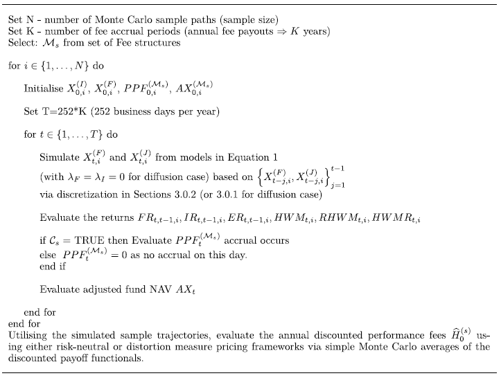
6. Monte Carlo Actuarial Performance Fee Pricing Case Studies
In this section, we will set out the scenarios and case studies to be performed in order to assess the behaviour of the different classes of fee fund structures and how the analysis of such fee funds, when priced as option-like derivative payoffs are affected by the type of pricing methodology applied. This will allow us to study the utility of different performance fee mechanisms under each pricing framework.
To perform studies on fee performance and pricing, we need to obtain several key pieces of data that relate to both the fund management and structure, the reference benchmark used to assess performance of the fund and the fee structures used for fund management compensation. Furthermore, we also need to obtain key market variables for calibration of our pricing models in Equation (1) which includes specifications of key aspects such as discounting interest rate references used and how we estimated NAV model parameters such as volatilities $\sigma _F$
and
$\sigma _F$
and $\sigma _I$
, correlation
$\sigma _I$
, correlation $\sigma _{FI}$
, as well as other parameters appearing in Equation (1).
$\sigma _{FI}$
, as well as other parameters appearing in Equation (1).
6.1 Case study fund selections
The case study undertaken will explore an application based on the three JP Morgan funds run in Luxemburg which are Europe Research Enhanced Index Equity and Income Opportunity Plus appearing in the 2017 Prospectus (J.P.Morgan Asset Management, 2017) and Income Opportunity appearing on 2021 Prospectus (J.P.Morgan Asset Management, 2021). The details of each fund are shown in Table 2. We note that the selection of these illustrative funds provides an anchoring for the scenario case studies explored for various fee mechanisms, to be based in a realistic practical framework.
Table 2. Fund details used in the case studies.
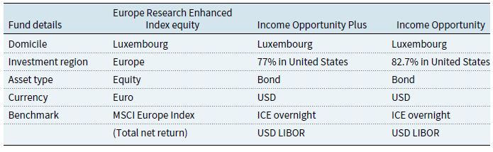
According to the 2017 (J.P.Morgan Asset Management, 2017) and 2021 (J.P.Morgan Asset Management, 2021) prospectuses, model $\mathcal{M}_1$
is applied to Europe Research Enhanced Index Equity (share class I) while model
$\mathcal{M}_1$
is applied to Europe Research Enhanced Index Equity (share class I) while model $\mathcal{M}_2$
is applied to Income Opportunity Plus (2017) as well as Income Opportunity (2021).
$\mathcal{M}_2$
is applied to Income Opportunity Plus (2017) as well as Income Opportunity (2021).
For Europe Research Enhanced Index Equity (share class I), the fee rates are $MF=0.16\%$
,
$MF=0.16\%$
, $OF=0.19\%$
and
$OF=0.19\%$
and $PF=10\%$
. For both Income Opportunity Plus and Income Opportunity, the values are
$PF=10\%$
. For both Income Opportunity Plus and Income Opportunity, the values are $MF=0.55\%$
,
$MF=0.55\%$
, $OF=0.11\%$
and
$OF=0.11\%$
and $PF=20\%$
. The summary of fund fees together with their fee mechanism is shown in Table 3. All Fund NAVs including MSCI Europe Index NAVs are displayed in Figure 1.
$PF=20\%$
. The summary of fund fees together with their fee mechanism is shown in Table 3. All Fund NAVs including MSCI Europe Index NAVs are displayed in Figure 1.
Table 3. The selected funds together with their share class and fee structures.
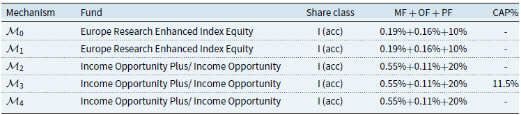
Note: (acc) means the share class of interest does not pay dividends. Earned income is reinvested in the NAV (J.P.Morgan Asset Management, 2017).

Figure 1 Fund and benchmark NAVs.
Although model $\mathcal{M}_3$
is defined in the 2017 Prospectus (J.P.Morgan Asset Management, 2017), the mechanism is not actually applied to Income Opportunity Plus, but it is applied to US opportunistic Long-Short Equity which is not included in this study as the fund and its benchmark data is not sufficiently available to undertake a complete study. The CAP at
$\mathcal{M}_3$
is defined in the 2017 Prospectus (J.P.Morgan Asset Management, 2017), the mechanism is not actually applied to Income Opportunity Plus, but it is applied to US opportunistic Long-Short Equity which is not included in this study as the fund and its benchmark data is not sufficiently available to undertake a complete study. The CAP at $11.5\%$
is indicated in the 2017 Prospectus (J.P.Morgan Asset Management, 2017) to apply to the US opportunistic Long-Short Equity. Instead, to study model
$11.5\%$
is indicated in the 2017 Prospectus (J.P.Morgan Asset Management, 2017) to apply to the US opportunistic Long-Short Equity. Instead, to study model $\mathcal{M}_3$
in comparison with model
$\mathcal{M}_3$
in comparison with model $\mathcal{M}_2$
, we apply the same CAP at
$\mathcal{M}_2$
, we apply the same CAP at $11.5\%$
, shown in Table 3, to Income Opportunity Plus and Income Opportunity. Model
$11.5\%$
, shown in Table 3, to Income Opportunity Plus and Income Opportunity. Model $\mathcal{M}_4$
is also developed in order to analyse model
$\mathcal{M}_4$
is also developed in order to analyse model $\mathcal{M}_2$
.
$\mathcal{M}_2$
.
In this work, the period of study is set to be three years. We assume the period is sufficiently long to accurately measure the long-term performance of a mutual fund so that the assessment of performance is not affected solely by the short-term fluctuations in market cycles over a single business cycle in the equity markets.
6.2 Discounting interest rates
We assume the investor can deposit money in a secure “bank account” and earn a risk-free interest rate, when not investing. In this section, we discuss the bank account yields and we will differentiate between the Eurozone and the US investor.
For Europe Research Enhanced Index which invested in the European region, its risk-free rate is set to equal the yield of AAA-rated Euro-area central government bonds with one-year term to maturity and is assumed to be fixed throughout the period of our study. The rate on 25th July 2017 is $-0.70\%$
(European Central Bank, 2020). We use the rate quoted in year 2017 since the fund with performance fee structure was available in year 2017 and the fee structure was cancelled in the following year.
$-0.70\%$
(European Central Bank, 2020). We use the rate quoted in year 2017 since the fund with performance fee structure was available in year 2017 and the fee structure was cancelled in the following year.
During recent years, all yields in this region are negative for various reasons related to the current macroeconomy of the region and geopolitical factors that may have caused uncertainty in this economic region. Negative yielding rates on fixed income products are a recent phenomenon that would typically discourage both fund manager and investor to invest in such instruments in cash-based bank accounts, however for large capital investments, they are seen as somewhat of a safer option for investing even with this negative yield than keeping money in more volatile assets such as equities or commodities. They can still offer a long-term safe haven for large amounts of total assets that are required to be deployed for investment purposes even during high volatility periods of the markets. Therefore, we still assume the investor and manager choose to keep riskless assets in a bank account with risk-free rate although the risk-free rate itself is negative.
For Income Opportunity Plus and Income Opportunity which invested most in the American region, the United States Treasury bond yield curve rates with maturity time of one year are used as its risk-free rate and are assumed to be fix throughout three years of our study period. The rate for Income Opportunity Plus is at $1.24\%$
quoted on 30th June 2017 (Daily Treasury Yield Curve Rates). We use the rate quoted in year 2017 since the fund was available during the year, and later, it was merged with Income Opportunity in year 2018. As for Income Opportunity, the risk-free rate is
$1.24\%$
quoted on 30th June 2017 (Daily Treasury Yield Curve Rates). We use the rate quoted in year 2017 since the fund was available during the year, and later, it was merged with Income Opportunity in year 2018. As for Income Opportunity, the risk-free rate is $0.09\%$
on 1st July 2021 (Daily Treasury Yield Curve Rates). The rate quoted in year 2021 is adopted since the fund is available in J.P.Morgan Prospectus of year 2021 (J.P.Morgan Asset Management, 2021). All parameter values of risk-free rates are summarised in Table 4.
$0.09\%$
on 1st July 2021 (Daily Treasury Yield Curve Rates). The rate quoted in year 2021 is adopted since the fund is available in J.P.Morgan Prospectus of year 2021 (J.P.Morgan Asset Management, 2021). All parameter values of risk-free rates are summarised in Table 4.
Table 4. Fund and fee parameter values.
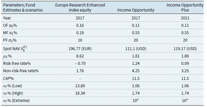
Note 1: Estimated model parameters for $\mu _F$
are obtained over the 3-year data history. The estimated
$\mu _F$
are obtained over the 3-year data history. The estimated $\sigma _F$
low and high values were estimated based on a 1-year sliding window and the lowest historical estimate and highest historical estimates were used in the scenarios studied.
$\sigma _F$
low and high values were estimated based on a 1-year sliding window and the lowest historical estimate and highest historical estimates were used in the scenarios studied.
Note 2: While the spot NAVs 196.77 (EUR) and 111.1 (USD) were the NAVs on 25 July 2017, 119.17 USD was the NAV on 11 August 2021 (Morgan).
Note 3: setting the extreme scenario volatility at $10^*\%$
was not estimated from observed historical NAVs but set up in order to study the effect of CAP on model
$10^*\%$
was not estimated from observed historical NAVs but set up in order to study the effect of CAP on model $\mathcal{M}_3$
in an extreme scenario.
$\mathcal{M}_3$
in an extreme scenario.
7. Formulating Scenarios based on Estimation of the Stochastic NAV Model Parameters
The intention is to develop a set of scenarios to study the behaviour of fund fee structures under various pricing frameworks and to see how the fund fee structures behave in differing economic environments, as captured by various specified scenarios for the fund NAV parameters and corresponding reference benchmark model parameters.
In order to ensure that scenario specifications were realistic in nature, the manner in which the scenarios were selected was based on two stages:
-
statistical estimation of model parameters was performed to set a reference range on model parameters, based on the observed historical NAV fund performance data, see Figure 1.
-
model parameter estimates were then used to set a range of scenarios that allowed for testing of fee structure performance in various realistic good and bad scenarios.
As such, it is not the intention of this section of the paper to perfectly calibrate the models to the historical performance, but rather to obtain estimates for the model parameters for the fund and reference fund NAV processes that will allow for the scenarios to be meaningfully specified based on real data case studies. Both the diffusion and jump diffusion models were estimated based on moment-matching frameworks as outlined below.
7.1 Estimation of the diffusion components and construction of scenarios
For the development of the stochastic models used in the NAV dynamics, we will require to estimate certain model parameters. In Equation (1), $\mu _F$
is the annual mean return of fund, while
$\mu _F$
is the annual mean return of fund, while $\mu _I$
is the annual mean return of the benchmark index fund. The two parameters were calibrated based on the fund and benchmark data (Reference MorganMorgan; MSCI Europe Net EUR Historical Rates (MIEU00000NEU)) and their values are shown in Tables 4 and 5, respectively.
$\mu _I$
is the annual mean return of the benchmark index fund. The two parameters were calibrated based on the fund and benchmark data (Reference MorganMorgan; MSCI Europe Net EUR Historical Rates (MIEU00000NEU)) and their values are shown in Tables 4 and 5, respectively.
Table 5. Benchmark parameter values.
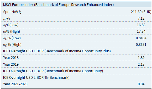
Note: The NAV 211.60 (EUR) is the benchmark NAV on 8 August 2017 (MSCI Europe Net EUR Historical Rates (MIEU00000NEU)).
Calibration of the pure diffusion models, which involved setting $\lambda _I=\lambda _F=0$
, was based on a moment-matching method of estimation of the discretised Lognormal models from Equation (3) for the fund and benchmark NAV processes. The estimated drift and volatility parameters in Table 4 are estimated based on the simple moment-matching approach from historical data from NAV data.
$\lambda _I=\lambda _F=0$
, was based on a moment-matching method of estimation of the discretised Lognormal models from Equation (3) for the fund and benchmark NAV processes. The estimated drift and volatility parameters in Table 4 are estimated based on the simple moment-matching approach from historical data from NAV data.
Given $Z$
a standard normal variable with
$Z$
a standard normal variable with $\mu$
and
$\mu$
and $\sigma \gt 0$
parameters. Then, the distribution of the random variable
$\sigma \gt 0$
parameters. Then, the distribution of the random variable $X=e^{\mu +\sigma Z}$
is the lognormal distribution with parameters
$X=e^{\mu +\sigma Z}$
is the lognormal distribution with parameters $\mu$
and
$\mu$
and $\sigma$
and the moment-matching equations solved are given by:
$\sigma$
and the moment-matching equations solved are given by:
 \begin{align} \mu =\ln \!\left ({\frac{\mu _{X}^{2}}{\sqrt{\mu _{X}^{2}+\sigma _{X}^{2}}}}\right ), \;\;\;\; \sigma ^{2} =\ln \!\left (1+{\frac{\sigma _{X}^{2}}{\mu _{X}^{2}}}\right ). \end{align}
Historical volatility and correlation are also used as parameters in Equation (3) to simulate NAVs of fund and benchmark. We estimate the annualised historical volatility rather than the implied volatility based on the justification that options are generally priced more fairly based on historical norms. The historical volatilities of each fund NAV, $\sigma _{F}$
, and each benchmark NAV,
$\sigma _{F}$
, and each benchmark NAV, $\sigma _{I}$
, and their correlation,
$\sigma _{I}$
, and their correlation, $\sigma _{FI}$
, as well as tracking error
$\sigma _{FI}$
, as well as tracking error $\sigma _{F-I}$
, are estimated based on available NAV data. The historical volatility period is set to be three years, and one year is assumed to consist of 252 trading days. The following steps are used to estimate
$\sigma _{F-I}$
, are estimated based on available NAV data. The historical volatility period is set to be three years, and one year is assumed to consist of 252 trading days. The following steps are used to estimate $\sigma _F$
,
$\sigma _F$
, $\sigma _I$
, and
$\sigma _I$
, and $\sigma _{FI}$
:
$\sigma _{FI}$
:
-
1. Calculate day-to-day returns
$DR_F$
and
$DR_I$
of the fund and benchmark, respectively. -
2. Calculate the standard deviation of the fund return
$\sigma _{DRF}$
, benchmark return
$\sigma _{DRI}$
, and their correlation
$\sigma _{DRFI}$
during the historical volatility period. -
3. Annualise the standard deviations based on the selected number of trading days which is 252 days, that is,
$\sigma _{F}=\sigma _{DRF}\sqrt{252}$
,
$\sigma _{I}=\sigma _{DRI}\sqrt{252}$
, and
$\sigma _{FI}=\sigma _{DRFI} (252)$


For $\sigma _{F-I}$
, we adopt the formula below:
$\sigma _{F-I}$
, we adopt the formula below: $\sigma _{F-I}=\sqrt{\sigma ^2_F+\sigma ^2_I-2\sigma _F\sigma _I\sigma _{FI}}$
For models $\mathcal{M}_0$
and
$\mathcal{M}_0$
and $\mathcal{M}_1$
, we provide two scenarios (low and high estimates) of volatilities and correlations to analyse the sensitivity of fees under the different financial market conditions. For models
$\mathcal{M}_1$
, we provide two scenarios (low and high estimates) of volatilities and correlations to analyse the sensitivity of fees under the different financial market conditions. For models $\mathcal{M}_2$
,
$\mathcal{M}_2$
, $\mathcal{M}_3$
, and
$\mathcal{M}_3$
, and $\mathcal{M}_4$
, one more extreme scenario is added to analyse the effect of CAP on model
$\mathcal{M}_4$
, one more extreme scenario is added to analyse the effect of CAP on model $\mathcal{M}_3$
.
$\mathcal{M}_3$
.
The values of $\sigma _{F}$
are provided in Table 4, while values for
$\sigma _{F}$
are provided in Table 4, while values for $\sigma _{I}$
,
$\sigma _{I}$
, $\sigma _{FI}$
, and
$\sigma _{FI}$
, and $\sigma _{F-I}$
are provided in Table 5.
$\sigma _{F-I}$
are provided in Table 5.
7.2 Jump component parameter estimation and scenario specifications
In this section, the jump diffusion model calibration and scenario specifications are discussed. The focus will be on the discretised version in Equation (7), and the procedure adopted for model estimation. There are numerous approaches proposed in the literature to calibrate a jump diffusion model, see Cont & Tankov (Reference Cont and Tankov2004) and Schoutens et al. (Reference Schoutens, Simons and Tistaert2003). In this work, we have opted to use a framework developed in Matlab version “9.12.0.1884302 (R2022a)” framework (https://www.mathworks.com/company/newsletters/articles/estimating-market-implied-value-with-jump-diffusion-models.html) with adaption to the small time scale approximation considered in Equation (7).
For the jump diffusion models, we have based the diffusion components of these models on the method of moments results discussed previously. Below we will discuss how to estimate the parameters for the jump components. Under this estimation procedure, one first segments the return series into change point segmentations, see the optimal selections of the estimated segmentation’s obtained in each time series in Figure 2. One has a choice to segment the price process according to the trend changes induced by a jump or to alternatively work with the detrended log-returns process via a segmentation of volatility changes (std. dev.) or Root-Mean-Square error changes. We utilised a detrending of the price process, but explored the log-returns segmentation also and found very similar results in the location of detected jumps. The number of optimal change points detected were explored between 1 and 50 changes, and the optimal choices are presented in the figure for each NAV data set. The criterion used for selecting optimal change point counts was an AIC criterion on the fitted local trend models as depicted and the optimal segmentation order was selected to minimised the AIC.
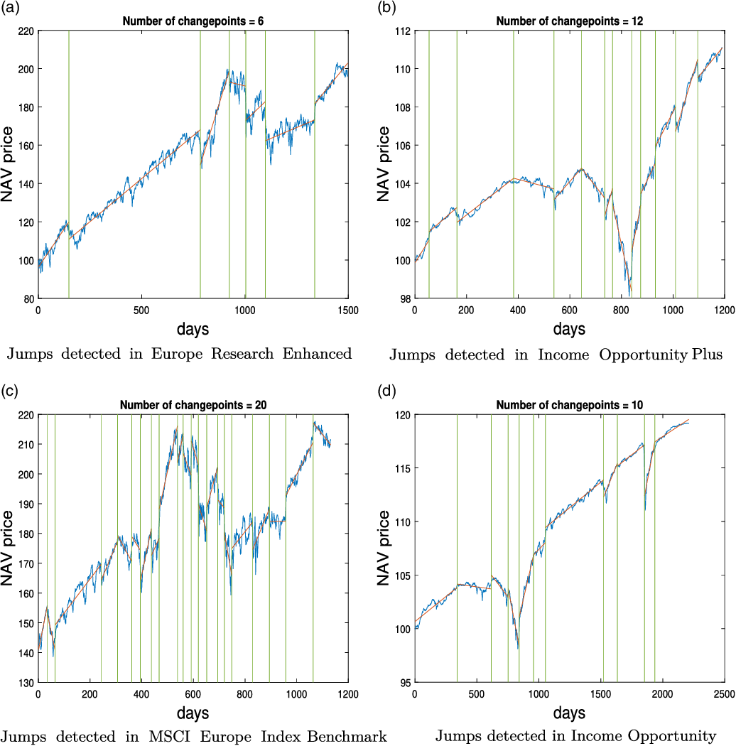
Figure 2 Jumps detected in fund and benchmark NAVs.
For the jump diffusion models, $\lambda _F\gt 0$
,
$\lambda _F\gt 0$
, $\lambda _I\gt 0$
were estimated based on the number of detected jumps annually which produced and average annualised jump intensity for each fund estimated to be: Europe Research Enhanced
$\lambda _I\gt 0$
were estimated based on the number of detected jumps annually which produced and average annualised jump intensity for each fund estimated to be: Europe Research Enhanced $\lambda _F = 0.003$
; Income Opportunity
$\lambda _F = 0.003$
; Income Opportunity $\lambda _F = 0.0033$
; Income Opportunity Plus
$\lambda _F = 0.0033$
; Income Opportunity Plus $\lambda _F = 0.008$
; and benchmark MSCI Europe Index
$\lambda _F = 0.008$
; and benchmark MSCI Europe Index $\lambda _F = 0.012$
. These values were then used to set the probability of
$\lambda _F = 0.012$
. These values were then used to set the probability of $B=1$
in small time scale representation Equation (7). Furthermore, the distribution of the jump sizes over time is plotted in the following Figure 3. The probability of an upward move (
$B=1$
in small time scale representation Equation (7). Furthermore, the distribution of the jump sizes over time is plotted in the following Figure 3. The probability of an upward move ( $p$
) was estimated to be: Europe Research Enhanced
$p$
) was estimated to be: Europe Research Enhanced $p=0.2$
; Income Opportunity
$p=0.2$
; Income Opportunity $p=0.7$
; Income Opportunity Plus
$p=0.7$
; Income Opportunity Plus $p=0.3$
; and benchmark MSCI Europe Index
$p=0.3$
; and benchmark MSCI Europe Index $p=0.5$
. The intensities for the jumps were estimated to be: Europe Research Enhanced
$p=0.5$
. The intensities for the jumps were estimated to be: Europe Research Enhanced $\eta _1=6,\eta _2=1.2$
; Income Opportunity
$\eta _1=6,\eta _2=1.2$
; Income Opportunity $\eta _1=1.4,\eta _2=3.3$
; Income Opportunity Plus
$\eta _1=1.4,\eta _2=3.3$
; Income Opportunity Plus $\eta _1=3,\eta _2=1.5$
; and benchmark MSCI Europe Index
$\eta _1=3,\eta _2=1.5$
; and benchmark MSCI Europe Index $\eta _1=2.2,\eta _2=1.8$
.
$\eta _1=2.2,\eta _2=1.8$
.
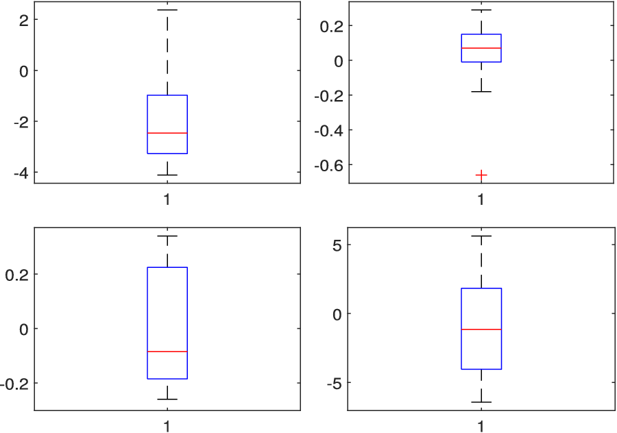
Figure 3 Distribution of jump sizes. Top left panel: Europe Research Enhanced; Top right panel: Income Opportunity; Bottom left panel: Income Opportunity Plus; Bottom right panel: MSCI Europe Index Benchmark.
One can observe from this that for some NAV processes there was a greater negative support and for others a greater positive support in jumps, so there is no clear consensus in this case study as to a strictly greater magnitude of downward moves and chance of downward moves in these markets in general. We note that compared to other studies that have been undertaken in equity markets that tend to indicate a greater support for larger negative jumps as compared to positive jumps this is a difference for these markets under study in this work, see discussions in Kou (Reference Kou2007) and (Reference Kou2002). We suspect such findings will highly depend on the window of time studied and assets studied, and there is no definitive consensus that $p \gt 0.5$
in general or that the size of negative jumps should be greater than positive jumps, that is
$p \gt 0.5$
in general or that the size of negative jumps should be greater than positive jumps, that is $\frac{1}{\eta _1} \lt \frac{1}{\eta _2}$
for all periods and market cycles.
$\frac{1}{\eta _1} \lt \frac{1}{\eta _2}$
for all periods and market cycles.
We now point out that the analysis performed using these estimated parameter settings produced results that were very closely aligned with those obtained from the pure diffusion setting, due to the low chance of having any simulated jumps in the price process and the fact that when a jump was simulated, they did not lead to a significant change in the outcomes of the findings relative to the diffusion setting. Due to space, these results were omitted as they did not change the perspective learnt on fee fund structure and pricing behaviour compared to those already discovered from the diffusion model analysis.
We have therefore just focused on what we define as an extreme scenario for jump diffusion models which represents a case where jumps were more consequential in affecting the outcomes. This will better provide an indication of the influence of jumps in a market environment in which jumps had greater impact. For instance, this may be consistent with time periods like those in March 2020 at the start of the COVID-19 pandemic or consistent with those in May-June 2022 as inflation is rising and the Federal Reserve has significantly increased interest rates compared to historical changes, leading to either very large declines in asset prices or increases in asset prices as was the case when stimulus support was announced after the initial COVID-19 lockdowns occurred.
Consequently, in the scenarios developed we decided to simulate the chance of an upward or downward move as equal in magnitude for upward or downward moves, setting $p=0.5$
.
$p=0.5$
.
8. Scenario Case Study Pricing Results
The detailed steps of the Monte Carlo simulations performed for each study are provided in section 5.5 and Algorithm 1. Furthermore, the case study model settings are provided in section 6. Both these pricing methods (with jump diffusion models & pure diffusion models) are studied below in a sequence of illustrative case studies. In order to perform the simulation studies, we first had to determine a reasonable estimate for the number of trials of Monte Carlo simulations to run in order to obtain an accurate pricing outcome. To select the number of Monte Carlo trials, we utilise a criterion based on setting a threshold on the coefficient of variation ( $CV$
) of the estimated mean discounted performance fee of each simulation. We required that it was less than 0.2, corresponding to an acceptable
$CV$
) of the estimated mean discounted performance fee of each simulation. We required that it was less than 0.2, corresponding to an acceptable $CV$
range consistent with those proposed in Reed et al. (Reference Reed, Lynn and Meade2002). As a reference, we used the findings from the case of the non-jump setup under pricing method 1, which corresponded after rounding upwards, to be conservative, to a total of 1,000 Monte Carlo simulations being required to satisfy this criterion for each study.
$CV$
range consistent with those proposed in Reed et al. (Reference Reed, Lynn and Meade2002). As a reference, we used the findings from the case of the non-jump setup under pricing method 1, which corresponded after rounding upwards, to be conservative, to a total of 1,000 Monte Carlo simulations being required to satisfy this criterion for each study.
8.1 Results: Pricing method
$1$
(risk-neutral & no jumps)

We conduct three-year studies for the models with the selected fund. For each study, we price performance fee PF $\%$
, management and advisory fee MF
$\%$
, management and advisory fee MF $\%$
(shown in square brackets), operating and administrative fee OF
$\%$
(shown in square brackets), operating and administrative fee OF $\%$
(shown in parentheses) and tracking error
$\%$
(shown in parentheses) and tracking error $\%$
(shown in angle brackets). Furthermore, we also undertake an analysis of how the fee performance relates to profit performance. In this regard, we provide results that determine the return on investment ROI
$\%$
(shown in angle brackets). Furthermore, we also undertake an analysis of how the fee performance relates to profit performance. In this regard, we provide results that determine the return on investment ROI $\%$
(shown in curly brackets).
$\%$
(shown in curly brackets).
8.1.1 Models
$\mathcal{M}_0$
and
$\mathcal{M}_1$
on Europe Research Enhanced Index


Under pricing method 1, Figure 4 shows an example of simulated realisations of discounted cumulative performance fee for model $\mathcal{M}_0$
(left) and
$\mathcal{M}_0$
(left) and $\mathcal{M}_1$
(right) calculated by assuming risky interest rate, low fund volatility, low benchmark volatility, and low correlation as specified according to settings in section 6. Interestingly, the cumulative performance fee under model
$\mathcal{M}_1$
(right) calculated by assuming risky interest rate, low fund volatility, low benchmark volatility, and low correlation as specified according to settings in section 6. Interestingly, the cumulative performance fee under model $\mathcal{M}_1$
(right) is not monotonically increasing during the year like in case of model
$\mathcal{M}_1$
(right) is not monotonically increasing during the year like in case of model $\mathcal{M}_0$
(left) before being reset after 252 days as the performance fee is paid. This may be caused by the symmetric-penalised structure of the claw-back mechanism of model
$\mathcal{M}_0$
(left) before being reset after 252 days as the performance fee is paid. This may be caused by the symmetric-penalised structure of the claw-back mechanism of model $\mathcal{M}_1$
. Furthermore, the results of all scenarios for model
$\mathcal{M}_1$
. Furthermore, the results of all scenarios for model $\mathcal{M}_0$
are provided in Table 9 in the first set of columns, and those for model
$\mathcal{M}_0$
are provided in Table 9 in the first set of columns, and those for model $\mathcal{M}_1$
are provided in Table 9 in the second set of columns. For both models
$\mathcal{M}_1$
are provided in Table 9 in the second set of columns. For both models $\mathcal{M}_0$
and
$\mathcal{M}_0$
and $\mathcal{M}_1$
, annual MFs and OFs do not vary significantly and are close to 0.19
$\mathcal{M}_1$
, annual MFs and OFs do not vary significantly and are close to 0.19 $\%$
and 0.16
$\%$
and 0.16 $\%$
which is consistent with what is observed in practice for these funds. Note that, from the tables, the PFs under the same scenario of the two examples are
$\%$
which is consistent with what is observed in practice for these funds. Note that, from the tables, the PFs under the same scenario of the two examples are $5.97\%$
and
$5.97\%$
and $0.79\%$
, respectively, which is consistent with the daily cumulative fee average of the two models coloured in blue in Figure 4.
$0.79\%$
, respectively, which is consistent with the daily cumulative fee average of the two models coloured in blue in Figure 4.

Figure 4 Present value of cumulative performance fee (red) of Europe Research Enhanced Index Equity simulated via pricing method 1 together with the daily cumulative fee average (blue) plotted over 756 trading days (3 years).
As for PFs for $\mathcal{M}_0$
model, the values can vary in range
$\mathcal{M}_0$
model, the values can vary in range $5-7\%$
. The highest performance fee at
$5-7\%$
. The highest performance fee at $6.87\%$
falls into the scenario of high volatility (for both fund and benchmark), but low correlation under a negative discount rate. Nonetheless, the lowest performance fee at
$6.87\%$
falls into the scenario of high volatility (for both fund and benchmark), but low correlation under a negative discount rate. Nonetheless, the lowest performance fee at $5.71\%$
falls into the scenario of low volatility (for both fund and benchmark), but high correlation under high positive discount rate. By assuming ceteris paribus and varying only one variable at a time: either lowering correlations; increasing fund volatility; or increasing benchmark volatility, all possible individual changes result in higher PFs.
$5.71\%$
falls into the scenario of low volatility (for both fund and benchmark), but high correlation under high positive discount rate. By assuming ceteris paribus and varying only one variable at a time: either lowering correlations; increasing fund volatility; or increasing benchmark volatility, all possible individual changes result in higher PFs.
Regarding the returns of investment ROIs for $\mathcal{M}_0$
model, the values fall in range
$\mathcal{M}_0$
model, the values fall in range $8-9\%$
. The highest ROI at
$8-9\%$
. The highest ROI at $8.72\%$
given by the scenario of low fund volatility and low correlation, but high benchmark volatility under either positive or negative discount rates. On the contrary, the lowest ROI at
$8.72\%$
given by the scenario of low fund volatility and low correlation, but high benchmark volatility under either positive or negative discount rates. On the contrary, the lowest ROI at $8.64\%$
is given by the scenario of high fund volatility and high correlation, but low benchmark volatility under either positive or negative discount rates. By assuming ceteris paribus and varying only one variable at a time: either lowering fund volatility, lowering correlation, or increasing benchmark volatility, all possible individual changes result in higher ROIs. When considering the cost of investment relative to profit (PF per ROI), we found that the relative cost follows the PF trend, that is, highest at
$8.64\%$
is given by the scenario of high fund volatility and high correlation, but low benchmark volatility under either positive or negative discount rates. By assuming ceteris paribus and varying only one variable at a time: either lowering fund volatility, lowering correlation, or increasing benchmark volatility, all possible individual changes result in higher ROIs. When considering the cost of investment relative to profit (PF per ROI), we found that the relative cost follows the PF trend, that is, highest at $79.31\%$
when PF reaches maximum at
$79.31\%$
when PF reaches maximum at $6.87\%$
with ROI
$6.87\%$
with ROI $8.66\%$
and vice versa. Interestingly neither the highest PF nor the lowest one lead to the highest ROI.
$8.66\%$
and vice versa. Interestingly neither the highest PF nor the lowest one lead to the highest ROI.
This set of results therefore demonstrates that in the risk-neutral setting in which one models the NAV processes as pure diffusion models then the following takeaway considerations are important to the investor, regarding the impact of performance fees. Firstly, performance fees in the range of 5–7% are very substantial in nature, compared to just a simple buy and hold strategy which would yield around 10% returns in one simply bought an ETF on say the S&P500. In particular, by considering the plausible range of ROIs between $8-9\%$
, the ratios of PF per ROI fall between
$8-9\%$
, the ratios of PF per ROI fall between $65-80\%$
which is indeed extremely high for investors. This means most of investment profit is paid to a fund manager in terms of performance fee. Furthermore, the results show that when the fund NAV is increasingly uncorrelated with the reference index fund NAV performance, this will result in greater expense to the investor over the investment horizon. This indicates that investors would be best suited to select funds for which the reference index was suitably related and therefore correlated with the assets comprised in the investment fund. The subsequent findings, that increasing periods of volatility lead to higher performance fees, should only be acceptable to investors if the fund manager is able to ensure that either funds grow sufficiently in value during heightened volatility periods due to active management investment decisions or alternatively that invested capital is secured against large potential draw downs in highly volatile periods, where the investment fund manager may adopt a risk off investment attitude and therefore the higher performance fees indicate a reward for such fund stewardship.
$65-80\%$
which is indeed extremely high for investors. This means most of investment profit is paid to a fund manager in terms of performance fee. Furthermore, the results show that when the fund NAV is increasingly uncorrelated with the reference index fund NAV performance, this will result in greater expense to the investor over the investment horizon. This indicates that investors would be best suited to select funds for which the reference index was suitably related and therefore correlated with the assets comprised in the investment fund. The subsequent findings, that increasing periods of volatility lead to higher performance fees, should only be acceptable to investors if the fund manager is able to ensure that either funds grow sufficiently in value during heightened volatility periods due to active management investment decisions or alternatively that invested capital is secured against large potential draw downs in highly volatile periods, where the investment fund manager may adopt a risk off investment attitude and therefore the higher performance fees indicate a reward for such fund stewardship.
As for PFs and ROIs, although the values of PFs for $\mathcal{M}_1$
model varied from
$\mathcal{M}_1$
model varied from $0.8-0.9\%$
, which are drastically lower than the PFs for model
$0.8-0.9\%$
, which are drastically lower than the PFs for model $\mathcal{M}_0$
(factor of 10 times lower), the ROIs for
$\mathcal{M}_0$
(factor of 10 times lower), the ROIs for $\mathcal{M}_1$
model varied from
$\mathcal{M}_1$
model varied from $8.4-8.5\%$
which were only
$8.4-8.5\%$
which were only $3\%$
lower than the ROIs for model
$3\%$
lower than the ROIs for model $\mathcal{M}_0$
. This leads to a huge drop in the relative cost of investment (PF per ROI) for model
$\mathcal{M}_0$
. This leads to a huge drop in the relative cost of investment (PF per ROI) for model $\mathcal{M}_1$
to the range
$\mathcal{M}_1$
to the range $8.9-10.8\%$
(factor of 10 times lower than one for model
$8.9-10.8\%$
(factor of 10 times lower than one for model $\mathcal{M}_0$
). The same scenario which generated the highest PF for model
$\mathcal{M}_0$
). The same scenario which generated the highest PF for model $\mathcal{M}_0$
also yields both the highest PF and PF/ROI at
$\mathcal{M}_0$
also yields both the highest PF and PF/ROI at $0.9\%$
and
$0.9\%$
and $10.75\%$
, respectively, for model
$10.75\%$
, respectively, for model $\mathcal{M}_1$
. That also holds true in case of the lowest PF and PF/ROI at
$\mathcal{M}_1$
. That also holds true in case of the lowest PF and PF/ROI at $0.76\%$
and
$0.76\%$
and $8.94\%$
respectively.
$8.94\%$
respectively.
8.1.2 Models
$\mathcal{M}_2$
,
$\mathcal{M}_3$
, and
$\mathcal{M}_4$
on Income Opportunity Plus


An example of the movement of discounted cumulative performance fee over 3 years for model $\mathcal{M}_2$
(left),
$\mathcal{M}_2$
(left), $\mathcal{M}_3$
(middle), and
$\mathcal{M}_3$
(middle), and $\mathcal{M}_4$
(right) when interest rate is high and fund volatility is extremely high is shown in Figure 5. Similar to model
$\mathcal{M}_4$
(right) when interest rate is high and fund volatility is extremely high is shown in Figure 5. Similar to model $\mathcal{M}_1$
, the cumulative performance fee under models
$\mathcal{M}_1$
, the cumulative performance fee under models $\mathcal{M}_2$
,
$\mathcal{M}_2$
, $\mathcal{M}_3$
, and
$\mathcal{M}_3$
, and $\mathcal{M}_4$
are all not monotonically increasing during each year before being reset to zero after 252 days. This results from symmetric-penalised structure of the claw-back mechanism which is used as the baseline mechanism of the three models. Interestingly, in Figure 7(c), the first-year PF of model
$\mathcal{M}_4$
are all not monotonically increasing during each year before being reset to zero after 252 days. This results from symmetric-penalised structure of the claw-back mechanism which is used as the baseline mechanism of the three models. Interestingly, in Figure 7(c), the first-year PF of model $\mathcal{M}_4$
paid at the end of the year is above
$\mathcal{M}_4$
paid at the end of the year is above $1.5\%$
which is significantly higher than PFs of the later two years which are clearly lower than
$1.5\%$
which is significantly higher than PFs of the later two years which are clearly lower than $0.5\%$
. This may be due to the effect of HWM condition on the first year which may set the watermark to be too high to catch in the following years.
$0.5\%$
. This may be due to the effect of HWM condition on the first year which may set the watermark to be too high to catch in the following years.

Figure 5 Present value of cumulative $\%$
performance fees (red) of Income Opportunity Plus simulated via pricing method 1 together with the daily cumulative
$\%$
performance fees (red) of Income Opportunity Plus simulated via pricing method 1 together with the daily cumulative $\%$
fee average (blue) plotted over 756 trading days (3 years).
$\%$
fee average (blue) plotted over 756 trading days (3 years).
In addition, Table 10 reveals the results for model $\mathcal{M}_2$
,
$\mathcal{M}_2$
, $\mathcal{M}_3$
, and
$\mathcal{M}_3$
, and $\mathcal{M}_4$
when applied to the Income opportunity Plus fund, under pricing method 1. It is obvious that MFs and OFs remain nearly stable across all scenarios around
$\mathcal{M}_4$
when applied to the Income opportunity Plus fund, under pricing method 1. It is obvious that MFs and OFs remain nearly stable across all scenarios around $0.55\%$
and
$0.55\%$
and $0.11\%$
, respectively, which are consistent with the rates the company promised in the fund investor information.
$0.11\%$
, respectively, which are consistent with the rates the company promised in the fund investor information.
By considering results under different estimated values of volatility (low and high), PFs are varied from $0.1-0.3\%$
for models
$0.1-0.3\%$
for models $\mathcal{M}_2$
,
$\mathcal{M}_2$
, $\mathcal{M}_3$
, and
$\mathcal{M}_3$
, and $\mathcal{M}_4$
. In fact,
$\mathcal{M}_4$
. In fact, $\mathcal{M}_2$
,
$\mathcal{M}_2$
, $\mathcal{M}_3$
give exactly the same results under these two values (low and high) volatility.
$\mathcal{M}_3$
give exactly the same results under these two values (low and high) volatility. $\mathcal{M}_4$
yields a bit higher PFs than
$\mathcal{M}_4$
yields a bit higher PFs than $\mathcal{M}_2$
in all scenarios. Again, by assuming Ceteris Paribus and varying only one variable, either an increase in fund volatility or a decrease in discount rate lead to an increase in PFs for all scenarios. Under volatility values estimated from the NAV data, we see no effect of CAP on model
$\mathcal{M}_2$
in all scenarios. Again, by assuming Ceteris Paribus and varying only one variable, either an increase in fund volatility or a decrease in discount rate lead to an increase in PFs for all scenarios. Under volatility values estimated from the NAV data, we see no effect of CAP on model $\mathcal{M}_3$
; however, once the volatility was increased to reach
$\mathcal{M}_3$
; however, once the volatility was increased to reach $10\%$
, under the same scenario, PF for model
$10\%$
, under the same scenario, PF for model $\mathcal{M}_3$
are much lower than one for model
$\mathcal{M}_3$
are much lower than one for model $\mathcal{M}_2$
and
$\mathcal{M}_2$
and $\mathcal{M}_4$
.
$\mathcal{M}_4$
.
As for ROIs and PF/ROIs for models $\mathcal{M}_2$
,
$\mathcal{M}_2$
, $\mathcal{M}_3$
and
$\mathcal{M}_3$
and $\mathcal{M}_4$
, the ROIs and PF/ROIs varied from
$\mathcal{M}_4$
, the ROIs and PF/ROIs varied from $1.23-1.24\%$
and
$1.23-1.24\%$
and $12.5-21.2\%$
, respectively, under these two values (low and high) volatility. In fact, the ROI results of models
$12.5-21.2\%$
, respectively, under these two values (low and high) volatility. In fact, the ROI results of models $\mathcal{M}_2$
–
$\mathcal{M}_2$
– $\mathcal{M}_4$
are very close to each other (different by only
$\mathcal{M}_4$
are very close to each other (different by only $0.01-0.02\%$
). Again once the volatility was increased to reach
$0.01-0.02\%$
). Again once the volatility was increased to reach $10\%$
, under the same scenario, by considering the relative cost of investment (PF/ROI), it reveals that the effect of CAP does reduce the relative cost of model
$10\%$
, under the same scenario, by considering the relative cost of investment (PF/ROI), it reveals that the effect of CAP does reduce the relative cost of model $\mathcal{M}_3$
significantly when we compare the model relative cost against ones for model
$\mathcal{M}_3$
significantly when we compare the model relative cost against ones for model $\mathcal{M}_2$
and
$\mathcal{M}_2$
and $\mathcal{M}_4$
.
$\mathcal{M}_4$
.
8.1.3 Models
$\mathcal{M}_2$
,
$\mathcal{M}_3$
, and
$\mathcal{M}_4$
on Income Opportunity


After pricing method 1 is applied, Table 10 provides the results of all scenarios for model $\mathcal{M}_2$
,
$\mathcal{M}_2$
, $\mathcal{M}_3$
, and
$\mathcal{M}_3$
, and $\mathcal{M}_4$
on Income opportunity. Clearly, MFs and OFs are quite stable across all scenarios around
$\mathcal{M}_4$
on Income opportunity. Clearly, MFs and OFs are quite stable across all scenarios around $0.55\%$
and
$0.55\%$
and $0.11\%$
, respectively, and this is consistent with the rates indicated in the company prospectus.
$0.11\%$
, respectively, and this is consistent with the rates indicated in the company prospectus.
The range of PFs of all the models is from $0.4-0.5\%$
under different estimated values (low and high) of volatility. Most of PFs behaviours are very much the same as what we mentioned in the case of Income Opportunity Plus except that now
$0.4-0.5\%$
under different estimated values (low and high) of volatility. Most of PFs behaviours are very much the same as what we mentioned in the case of Income Opportunity Plus except that now $\mathcal{M}_4$
yields a bit lower PFs than
$\mathcal{M}_4$
yields a bit lower PFs than $\mathcal{M}_2$
in all scenarios.
$\mathcal{M}_2$
in all scenarios.
The ROI values and the effect of CAP on PF/ROI are quite similar to the results from Income Opportunity Plus except for the fact that the range of the relative cost (PF/ROI) falls between $30-37.5$
which is about twice of one on Income Opportunity Plus.
$30-37.5$
which is about twice of one on Income Opportunity Plus.
8.2 Results: Pricing method 2 (actuarial distortion pricing & jumps)
As in the previous section, we again conduct three-year studies for the models with the selected fund. For each study case, we price performance fee PF $\%$
, management and advisory fee MF
$\%$
, management and advisory fee MF $\%$
(shown in square brackets), operating and administrative fee OF
$\%$
(shown in square brackets), operating and administrative fee OF $\%$
(shown in parentheses), and also provide return on investment ROI
$\%$
(shown in parentheses), and also provide return on investment ROI $\%$
(shown in curly brackets) under pricing method 2. Results for these case studies are developed in the following section.
$\%$
(shown in curly brackets) under pricing method 2. Results for these case studies are developed in the following section.
8.2.1 Models
$\mathcal{M}_0$
and
$\mathcal{M}_1$
on Europe Research Enhanced Index


By adopting the pricing method 2, an example of realisations of discounted cumulative performance fee for model $\mathcal{M}_0$
(left) and
$\mathcal{M}_0$
(left) and $\mathcal{M}_1$
(right), calculated by assuming risky interest rate, low fund volatility, low benchmark volatility, and low correlation, is provided in Figure 6. Similar to the example of model
$\mathcal{M}_1$
(right), calculated by assuming risky interest rate, low fund volatility, low benchmark volatility, and low correlation, is provided in Figure 6. Similar to the example of model $\mathcal{M}_1$
under pricing method 1, the cumulative performance fee shows non-monotonically increasing behaviour during each year which is directly a result of the penalty structure of the claw-back mechanism. The results for all scenarios are given in Table 11. For both models
$\mathcal{M}_1$
under pricing method 1, the cumulative performance fee shows non-monotonically increasing behaviour during each year which is directly a result of the penalty structure of the claw-back mechanism. The results for all scenarios are given in Table 11. For both models $\mathcal{M}_0$
and
$\mathcal{M}_0$
and $\mathcal{M}_1$
, annual MFs and OFs are both larger than the rates indicated in the prospectus at 0.19
$\mathcal{M}_1$
, annual MFs and OFs are both larger than the rates indicated in the prospectus at 0.19 $\%$
and 0.16
$\%$
and 0.16 $\%$
, respectively. MF values were in the range
$\%$
, respectively. MF values were in the range $0.22-0.24\%$
, and OF values were in the range
$0.22-0.24\%$
, and OF values were in the range $0.19-0.20\%$
which are quite stable regardless of any changes in the scenarios explored or fee models studied.
$0.19-0.20\%$
which are quite stable regardless of any changes in the scenarios explored or fee models studied.

Figure 6 Present value of cumulative % performance fee (red) of Europe Research Enhanced Index Equity simulated via pricing method 2 together with the daily cumulative % fee average (blue) plotted over 756 trading days (3 years).
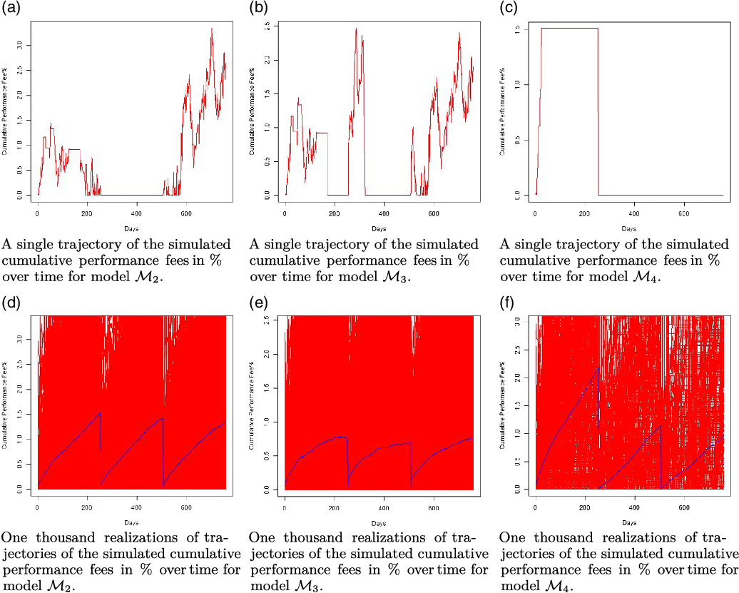
Figure 7 Present value of cumulative % performance fee (red) of Income Opportunity Plus simulated via pricing method 2 together with the daily cumulative % fee average (blue) plotted over 756 trading days (3 years).
Under pricing method 2, the values of PFs for $\mathcal{M}_0$
model were found to be between
$\mathcal{M}_0$
model were found to be between $7\%$
and
$7\%$
and $9\%$
, while those for
$9\%$
, while those for $\mathcal{M}_1$
model were between
$\mathcal{M}_1$
model were between $1.3\%$
and
$1.3\%$
and $1.5\%$
. All PFs derived from the two models under pricing method 2 are significantly larger than ones under pricing method 1. As for model
$1.5\%$
. All PFs derived from the two models under pricing method 2 are significantly larger than ones under pricing method 1. As for model $\mathcal{M}_0$
, the highest performance fee at
$\mathcal{M}_0$
, the highest performance fee at $8.58\%$
falls into the scenario of high volatility (of both fund and benchmark), but low correlation under a negative discount rate. The lowest performance fee is at
$8.58\%$
falls into the scenario of high volatility (of both fund and benchmark), but low correlation under a negative discount rate. The lowest performance fee is at $7.25\%$
derived from the scenario of low volatility (for both fund and benchmark), but high correlation under high positive discount rate. Ceteris Paribus the assumptions adopted, if we vary only one variable which is either lowering correlation, increasing fund volatility, or increasing benchmark volatility, all yield higher PFs. This pattern of PFs is consistent with what we found in the results of model
$7.25\%$
derived from the scenario of low volatility (for both fund and benchmark), but high correlation under high positive discount rate. Ceteris Paribus the assumptions adopted, if we vary only one variable which is either lowering correlation, increasing fund volatility, or increasing benchmark volatility, all yield higher PFs. This pattern of PFs is consistent with what we found in the results of model $\mathcal{M}_0$
under pricing method 1.
$\mathcal{M}_0$
under pricing method 1.
For PFs of $\mathcal{M}_1$
model under pricing method 2, the values of PFs varied between
$\mathcal{M}_1$
model under pricing method 2, the values of PFs varied between $1.3-1.5\%$
which was twice as large as those under pricing method 1. Under the same pricing method 2, we found a similar pattern in the PFs, namely that
$1.3-1.5\%$
which was twice as large as those under pricing method 1. Under the same pricing method 2, we found a similar pattern in the PFs, namely that $\mathcal{M}_1$
was much lower than those obtained for
$\mathcal{M}_1$
was much lower than those obtained for $\mathcal{M}_0$
(7 times lower). Indeed, the behaviour of PFs of
$\mathcal{M}_0$
(7 times lower). Indeed, the behaviour of PFs of $\mathcal{M}_1$
is the same as the pattern we found in the case of pricing method 1. Note that the highest PF is at
$\mathcal{M}_1$
is the same as the pattern we found in the case of pricing method 1. Note that the highest PF is at $1.49\%$
and the lowest was at
$1.49\%$
and the lowest was at $1.34\%$
. Both extremes appeared in the same scenarios as in the case of model
$1.34\%$
. Both extremes appeared in the same scenarios as in the case of model $\mathcal{M}_0$
.
$\mathcal{M}_0$
.
As for the ROIs of $\mathcal{M}_0$
and
$\mathcal{M}_0$
and $\mathcal{M}_1$
models, the ROI values are slightly varied between
$\mathcal{M}_1$
models, the ROI values are slightly varied between $17.30-17.33\%$
and
$17.30-17.33\%$
and $17.02-17.04\%$
, respectively. However, when considering the cost of investment relative to profit (PF per ROI), PF/ROI for
$17.02-17.04\%$
, respectively. However, when considering the cost of investment relative to profit (PF per ROI), PF/ROI for $\mathcal{M}_0$
model is at least five times higher than one for
$\mathcal{M}_0$
model is at least five times higher than one for $\mathcal{M}_1$
model given the same scenario.
$\mathcal{M}_1$
model given the same scenario.
8.2.2 Models
$\mathcal{M}_2$
,
$\mathcal{M}_3$
, and
$\mathcal{M}_4$
on Income Opportunity Plus


Figure 7 shows an example of discounted cumulative performance fee values over 3 years for model $\mathcal{M}_2$
(left),
$\mathcal{M}_2$
(left), $\mathcal{M}_3$
(middle), and
$\mathcal{M}_3$
(middle), and $\mathcal{M}_4$
(right) under the scenario of high interest rate and extremely high fund volatility. Similar to model
$\mathcal{M}_4$
(right) under the scenario of high interest rate and extremely high fund volatility. Similar to model $\mathcal{M}_1$
, the cumulative performance fee under models
$\mathcal{M}_1$
, the cumulative performance fee under models $\mathcal{M}_2$
,
$\mathcal{M}_2$
, $\mathcal{M}_3$
, and
$\mathcal{M}_3$
, and $\mathcal{M}_4$
are non-monotonically increasing during each year caused by symmetric-penalised structure of the claw-back mechanism which is used as the baseline mechanism of the three models. Interestingly, in Figure 7(c), it is now clear that, in this example of one single trajectory, the high watermark in the first year is too high to outperform in the following years as no performance fees are accrued at all, that is, cumulative performance fee remains at zero in the last two years. Moreover, Table 12 shows the results for model
$\mathcal{M}_4$
are non-monotonically increasing during each year caused by symmetric-penalised structure of the claw-back mechanism which is used as the baseline mechanism of the three models. Interestingly, in Figure 7(c), it is now clear that, in this example of one single trajectory, the high watermark in the first year is too high to outperform in the following years as no performance fees are accrued at all, that is, cumulative performance fee remains at zero in the last two years. Moreover, Table 12 shows the results for model $\mathcal{M}_2$
,
$\mathcal{M}_2$
, $\mathcal{M}_3$
, and
$\mathcal{M}_3$
, and $\mathcal{M}_4$
on Income opportunity (Plus) under pricing method 2. Across all scenarios and models, MFs and OFs remain close to
$\mathcal{M}_4$
on Income opportunity (Plus) under pricing method 2. Across all scenarios and models, MFs and OFs remain close to $0.55\%$
and
$0.55\%$
and $0.11\%$
, respectively, the rates indicated in the 2017 prospectus.
$0.11\%$
, respectively, the rates indicated in the 2017 prospectus.
Under the two estimated values of volatility (low and high), PFs of the three models varied from $0.5-1.5\%$
whose range is quite wide compared to one obtained when applying the three models under pricing method 1 (only between
$0.5-1.5\%$
whose range is quite wide compared to one obtained when applying the three models under pricing method 1 (only between $0.1$
and
$0.1$
and $0.3\%$
). One distinct relationship between
$0.3\%$
). One distinct relationship between $\mathcal{M}_2$
,
$\mathcal{M}_2$
, $\mathcal{M}_3$
is that now under the same the low or high volatility scenario, the two models do not yield the same result any longer. Instead, model
$\mathcal{M}_3$
is that now under the same the low or high volatility scenario, the two models do not yield the same result any longer. Instead, model $\mathcal{M}_3$
gives significantly lower PFs in all scenarios (at least two times lower). So, the effect of CAP on PFs is evidently stronger under pricing method 2.
$\mathcal{M}_3$
gives significantly lower PFs in all scenarios (at least two times lower). So, the effect of CAP on PFs is evidently stronger under pricing method 2. $\mathcal{M}_4$
results in quite higher PFs than
$\mathcal{M}_4$
results in quite higher PFs than $\mathcal{M}_2$
in low and high fund volatility scenarios but not in extremely high volatility one.
$\mathcal{M}_2$
in low and high fund volatility scenarios but not in extremely high volatility one.
Interestingly, we found one inconsistent pattern in PFs from models $\mathcal{M}_2$
as an increase in fund volatility from low to high does not increase PF values, for example, 1.04–1.02% and 1.08–1.06%, respectively. We believe that it is because the jump effect of NAV models dominates the effect from increasing volatility as the difference of the volatility values from the two scenarios (low and high) is just
$\mathcal{M}_2$
as an increase in fund volatility from low to high does not increase PF values, for example, 1.04–1.02% and 1.08–1.06%, respectively. We believe that it is because the jump effect of NAV models dominates the effect from increasing volatility as the difference of the volatility values from the two scenarios (low and high) is just $0.68\%$
.
$0.68\%$
.
However, the remaining scenarios generate the same pattern which is if we assume Ceteris Paribus and vary only one variable, that is, either by increasing fund volatility or by reducing discount rate, both cause an increase in PFs for all scenarios. The pattern in fact coincides with the pattern found in results of the three models under pricing method 1.
Regarding ROIs and PF/ROIs for models $\mathcal{M}_2$
,
$\mathcal{M}_2$
, $\mathcal{M}_3$
and
$\mathcal{M}_3$
and $\mathcal{M}_4$
, the ROIs and PF/ROIs fall in the ranges
$\mathcal{M}_4$
, the ROIs and PF/ROIs fall in the ranges $7.7-8.8\%$
and
$7.7-8.8\%$
and $6.8-20.5\%$
, respectively, under these two values (low and high) volatility. Under the same scenario, the ROI results for models
$6.8-20.5\%$
, respectively, under these two values (low and high) volatility. Under the same scenario, the ROI results for models $\mathcal{M}_2$
and
$\mathcal{M}_2$
and $\mathcal{M}_4$
are very close to each other (different by only
$\mathcal{M}_4$
are very close to each other (different by only $0.02-0.03 \%$
) while, for model
$0.02-0.03 \%$
) while, for model $\mathcal{M}_3$
, the ROI value is mildly lower (about
$\mathcal{M}_3$
, the ROI value is mildly lower (about $1\%$
) than the ROIs for models
$1\%$
) than the ROIs for models $\mathcal{M}_2$
and
$\mathcal{M}_2$
and $\mathcal{M}_4$
. When the volatility is extreme at
$\mathcal{M}_4$
. When the volatility is extreme at $10\%$
, by considering the relative cost of investment (PF/ROI) under the same scenario, the CAP condition is quite effective resulting in a huge drop of the relative cost for model
$10\%$
, by considering the relative cost of investment (PF/ROI) under the same scenario, the CAP condition is quite effective resulting in a huge drop of the relative cost for model $\mathcal{M}_3$
.
$\mathcal{M}_3$
.
8.2.3 Models
$\mathcal{M}_2$
,
$\mathcal{M}_3$
, and
$\mathcal{M}_4$
on Income Opportunity


Under pricing method 2, the results of all scenarios for model $\mathcal{M}_2$
,
$\mathcal{M}_2$
, $\mathcal{M}_3$
, and
$\mathcal{M}_3$
, and $\mathcal{M}_4$
on Income Opportunity are displayed in Table 12. In all scenarios, MFs and OFs are a bit higher than but still close to
$\mathcal{M}_4$
on Income Opportunity are displayed in Table 12. In all scenarios, MFs and OFs are a bit higher than but still close to $0.55\%$
and
$0.55\%$
and $0.11\%$
, respectively.
$0.11\%$
, respectively.
Under low and high estimated volatility, PFs of all the models fall in the range $0.7-1.7\%$
, a bit higher than one for Income Opportunity Plus. However, most of the patterns of PFs are very much the same as what we mentioned in the case of Income Opportunity Plus, under pricing method 2, except that now PFs of model
$0.7-1.7\%$
, a bit higher than one for Income Opportunity Plus. However, most of the patterns of PFs are very much the same as what we mentioned in the case of Income Opportunity Plus, under pricing method 2, except that now PFs of model $\mathcal{M}_4$
are lower than ones of model
$\mathcal{M}_4$
are lower than ones of model $\mathcal{M}_2$
in all scenarios, not just only in extreme fund volatility case.
$\mathcal{M}_2$
in all scenarios, not just only in extreme fund volatility case.
Moreover, the ROI values and the effect of CAP on PF/ROI are quite similar to the results from Income Opportunity Plus.
9. Discussion
In this section, we analyse the results obtained from the different case studies to assess the utility of the different fee structures in various economic scenarios under different stochastic model assumptions and pricing frameworks. We note the following details about the study results for these funds. The correlation between the Europe Research Enhanced Index Equity with its benchmark is quite high at nearly $90\%$
while its annualised tracking error is only
$90\%$
while its annualised tracking error is only $8-10\%$
(consistent with the high correlation). The volatility of the Income Opportunity Plus is quite low
$8-10\%$
(consistent with the high correlation). The volatility of the Income Opportunity Plus is quite low $(1-2\%)$
reflecting the fact that it is a bond-type fund while Europe Research Enhanced Index Equity and its benchmark volatilities are in a similar range, around
$(1-2\%)$
reflecting the fact that it is a bond-type fund while Europe Research Enhanced Index Equity and its benchmark volatilities are in a similar range, around $13-18\%$
. The range of variation, which we have considered for sensitivity analysis, may be not wide enough to explore all the possible scenarios, but this range reflects the actual range of uncertainty in the parameters.
$13-18\%$
. The range of variation, which we have considered for sensitivity analysis, may be not wide enough to explore all the possible scenarios, but this range reflects the actual range of uncertainty in the parameters.
Table 6. Sensitivity summary of performance fees for Europe Research Enhanced Index Equity. Table shows % amount of fee change and direction as well as the average Elasticity of the Performance Fees.
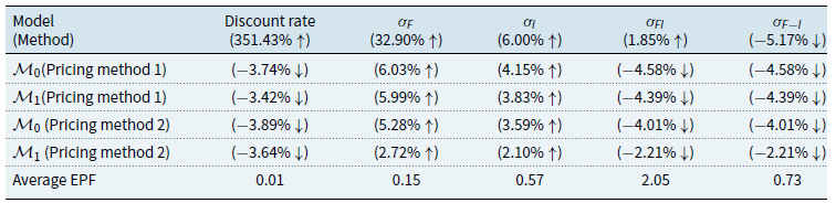
Table 7. Sensitivity summary of performance fees for Income Opportunity Plus and Income Opportunity.
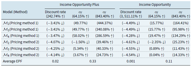
Ceteris Paribus, varying one-by-one, each component of the model parameters to produce various different market scenarios, we studied the movements of the fee values as % change, summarised in Tables 6 and 7. Moreover, to measure the effect of each parameter on PF values, we define the Elasticity of PF (EPF) to a change in parameter values as below:
 \begin{equation} EPF=\frac{\% change\,\,in\,\,PF\,\,value }{\% change\,\,in\,\,parameter\,\,value} \end{equation}
9.1 Performance fee sensitivity analysis for the Europe Research Enhanced Index Fund
As demonstrated in Table 6, for both models $\mathcal{M}_0$
and model
$\mathcal{M}_0$
and model $\mathcal{M}_1$
, under the two pricing methods, as discount rates increase, the PFs decrease. One can understand this effect in the following sense, when lowering discount rates, then the present value of the cash flow is higher resulting in the observed behaviour for the PFs.
$\mathcal{M}_1$
, under the two pricing methods, as discount rates increase, the PFs decrease. One can understand this effect in the following sense, when lowering discount rates, then the present value of the cash flow is higher resulting in the observed behaviour for the PFs.
Furthermore, one can observe from this analysis that PFs move in the same direction as both the fund and the benchmark volatility movements but in opposite direction to the correlation movements between the fund NAV and the reference benchmark funds NAV. Indeed, as we increase either fund or benchmark NAV volatilities, tracking error also increases as a result. Since PF follow the movement of tracking error; therefore, the PF moves in the same direction as both types of volatility.
In fact, the payoff of PF for model $\mathcal{M}_0$
is a spread option and, according to Pohjanpalo (Reference Pohjanpalo2013), as we increase tracking error, the price of the spread option increases. The explanation is that a larger variation in tracking error increases the chance that the payoff becomes positive and thus the performance fee increases. In case of model
$\mathcal{M}_0$
is a spread option and, according to Pohjanpalo (Reference Pohjanpalo2013), as we increase tracking error, the price of the spread option increases. The explanation is that a larger variation in tracking error increases the chance that the payoff becomes positive and thus the performance fee increases. In case of model $\mathcal{M}_1$
, the claw-back condition and symmetric-penalised structure mildly reduce the positive relation between tracking error and PF.
$\mathcal{M}_1$
, the claw-back condition and symmetric-penalised structure mildly reduce the positive relation between tracking error and PF.
Regarding the correlation parameter between the fund NAV and the reference benchmark fund NAV stochastic processes, it is clear given the diffusion and Lévy process model structures utilised, it is natural to observe that the fund and benchmark returns tend to move in the same direction as we increase their correlation positively. Consequently, their excess returns will diminish, thus decreasing the payoff for performance fees. This result is consistent with Pohjanpalo (Reference Pohjanpalo2013).
Clearly, under the two models, PF is most sensitive to the change in correlation between the fund NAV and the benchmark NAV for the case study of the European Research Enhanced Index. The justification for this conclusion is based on the fact that a small $2\%$
change in correlation causes almost
$2\%$
change in correlation causes almost $5\%$
change in magnitude for PF. This is consistent with the highest EPF at 2.05 which means a change in PF value is about two times the change in the correlation value. On the contrary, PF is the least sensitive to a change in discount rate as its EPF is only 0.01. We argue this type of analysis is directly useful for investors to be aware of to see which drivers or factors in the fund structure and performance fee structuring are most likely to increase their paid out fees each financial year.
$5\%$
change in magnitude for PF. This is consistent with the highest EPF at 2.05 which means a change in PF value is about two times the change in the correlation value. On the contrary, PF is the least sensitive to a change in discount rate as its EPF is only 0.01. We argue this type of analysis is directly useful for investors to be aware of to see which drivers or factors in the fund structure and performance fee structuring are most likely to increase their paid out fees each financial year.
9.2 Performance fee sensitivity analysis for Income Opportunity Plus and Income Opportunity Funds
We undertook a similar analysis, as just discussed, on the other two funds under study, the Income Opportunity Plus and Income Opportunity. Again, the PF decreases as one increase discount rate.
Since both the Income Opportunity Plus and Income Opportunity Funds used the LIBOR rates as their benchmark, the excess returns depend directly on $\sigma _{F}$
. Under pricing method 1, as
$\sigma _{F}$
. Under pricing method 1, as $\sigma _{F}$
increases, PFs of both funds increase in all the three models
$\sigma _{F}$
increases, PFs of both funds increase in all the three models $\mathcal{M}_2$
,
$\mathcal{M}_2$
, $\mathcal{M}_3$
, and
$\mathcal{M}_3$
, and $\mathcal{M}_4$
. Interestingly, under pricing method 2, PFs of the two funds are higher in
$\mathcal{M}_4$
. Interestingly, under pricing method 2, PFs of the two funds are higher in $\mathcal{M}_3$
and
$\mathcal{M}_3$
and $\mathcal{M}_4$
models, but lower in
$\mathcal{M}_4$
models, but lower in $\mathcal{M}_2$
model. We believe that this inconsistent pattern is caused by the dominance of jump effect of prices over the small increase of fund volatility
$\mathcal{M}_2$
model. We believe that this inconsistent pattern is caused by the dominance of jump effect of prices over the small increase of fund volatility $\sigma _{F}$
. However, when we raise
$\sigma _{F}$
. However, when we raise $\sigma _{F}$
even further (up
$\sigma _{F}$
even further (up $843.40\%$
), the positive-correlation trend reappears.
$843.40\%$
), the positive-correlation trend reappears.
Indeed, PFs under both funds are more sensitive to fund volatility than discount rate at average EPF of 0.33 against 0.02 for Income Opportunity Plus and 0.11 against 0.001 for Income Opportunity, respectively.
9.3 Pricing method variation
In this section, we study the effect of the pricing method applied to value the performance fees, from a risk-neutral pricing framework, versus an actuarial distortion pricing framework. The descriptive statistics summary of the PFs is shown in Table 8. All descriptive statistics point out that PFs calculated under the actuarial distortion pricing method 2 are higher than ones under pricing method 1. We believe, one driver of this discrepancy is the presence of the jump process components in the NAV models for the investment fund and the reference benchmark funds used under pricing method 2. The jump effect on the NAV simulation leads to higher excess returns as the gap between fund and benchmark NAVs tend to be larger than one under pricing method 1, where the NAV processes for the investment fund and reference benchmark fund are each pure diffusion processes. However, the standard deviation of PFs under pricing method 2 is lower.
Table 8. Descriptive statistics of PFs for Europe Research Enhanced Index under risk-neutral pricing (Pricing method 1) versus actuarial distortion pricing (Pricing method 2).
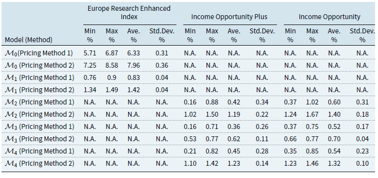
Table 9. % fees for Europe Research Enhanced Index Equity equipped with model $\mathcal{M}_0$
and
$\mathcal{M}_0$
and $\mathcal{M}_1$
generated by pricing method 1. No brackets: priced performance fee PF
$\mathcal{M}_1$
generated by pricing method 1. No brackets: priced performance fee PF $\%$
;
$\%$
; $[{\cdot}]$
brackets: priced management and advisory fee MF
$[{\cdot}]$
brackets: priced management and advisory fee MF $\%$
;
$\%$
; $({\cdot})$
brackets: priced operating and administrative fee OF
$({\cdot})$
brackets: priced operating and administrative fee OF $\%$
; and
$\%$
; and $\lt \cdot \gt$
brackets: priced tracking error
$\lt \cdot \gt$
brackets: priced tracking error $\%$
,
$\%$
, $\{\cdot \}$
: return on investment ROI
$\{\cdot \}$
: return on investment ROI $\%$
.
$\%$
.
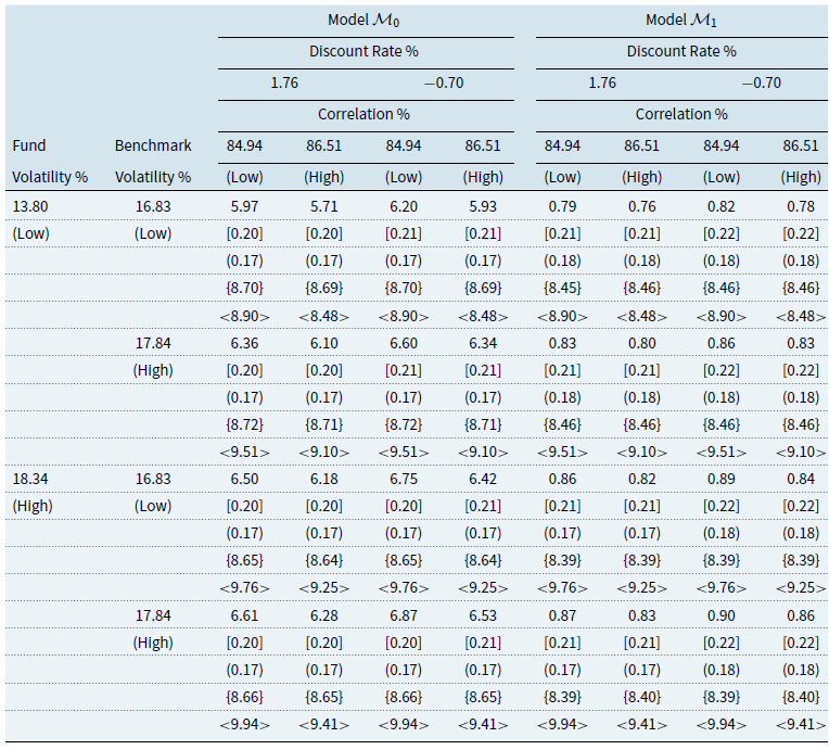
Table 10. % fees for Income Opportunity (Plus) equipped with model $\mathcal{M}_2$
,
$\mathcal{M}_2$
, $\mathcal{M}_3$
, and
$\mathcal{M}_3$
, and $\mathcal{M}_4$
generated by pricing method 1. No brackets: priced performance fee PF
$\mathcal{M}_4$
generated by pricing method 1. No brackets: priced performance fee PF $\%$
;
$\%$
; $[{\cdot}]$
brackets: priced management and advisory fee MF
$[{\cdot}]$
brackets: priced management and advisory fee MF $\%$
; and
$\%$
; and $({\cdot})$
brackets: priced operating and administrative fee OF
$({\cdot})$
brackets: priced operating and administrative fee OF $\%$
,
$\%$
, $\{\cdot \}$
: return on investment ROI
$\{\cdot \}$
: return on investment ROI $\%$
.
$\%$
.
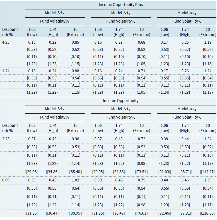
Table 11. % fees for Europe Research Enhanced Index Equity equipped with model $\mathcal{M}_0$
and
$\mathcal{M}_0$
and $\mathcal{M}_1$
generated by pricing method 2. No brackets: priced performance fee PF
$\mathcal{M}_1$
generated by pricing method 2. No brackets: priced performance fee PF $\%$
;
$\%$
; $[{\cdot}]$
brackets: priced management and advisory fee MF
$[{\cdot}]$
brackets: priced management and advisory fee MF $\%$
;
$\%$
; $({\cdot})$
brackets: priced operating and administrative fee OF
$({\cdot})$
brackets: priced operating and administrative fee OF $\%$
; and
$\%$
; and $\lt \cdot \gt$
brackets: priced tracking error
$\lt \cdot \gt$
brackets: priced tracking error $\%$
,
$\%$
, $\{\cdot \}$
: return on investment ROI
$\{\cdot \}$
: return on investment ROI $\%$
.
$\%$
.
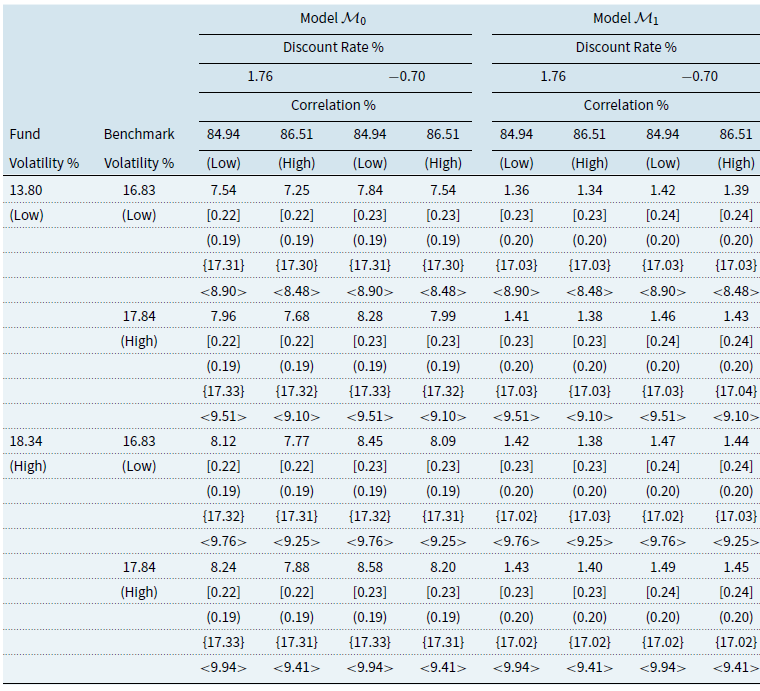
Table 12. % fees for Income Opportunity (Plus) equipped with model $\mathcal{M}_2$
,
$\mathcal{M}_2$
, $\mathcal{M}_3$
, and
$\mathcal{M}_3$
, and $\mathcal{M}_4$
generated by pricing method 2. No brackets: priced performance fee PF
$\mathcal{M}_4$
generated by pricing method 2. No brackets: priced performance fee PF $\%$
;
$\%$
; $[{\cdot}]$
brackets: priced management and advisory fee MF
$[{\cdot}]$
brackets: priced management and advisory fee MF $\%$
; and
$\%$
; and $({\cdot})$
brackets: priced operating and administrative fee OF
$({\cdot})$
brackets: priced operating and administrative fee OF $\%$
,
$\%$
, $\{\cdot \}$
: return on investment ROI
$\{\cdot \}$
: return on investment ROI $\%$
.
$\%$
.
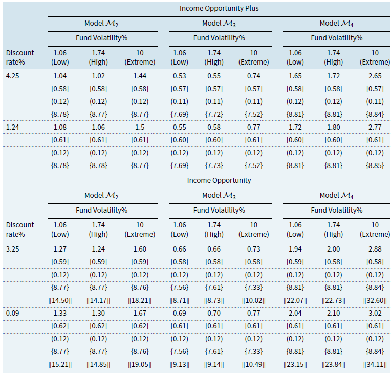
9.4 Analysis of fee model variations:
$\mathcal{M}_0$
,
$\mathcal{M}_1$
,
$\mathcal{M}_2$
,
$\mathcal{M}_3$
and
${\mathcal{M}}_4$


Having discussed the behaviour of the PF to various economic scenarios and pricing methods, we next move to a more detailed comparison between the different fee structures.
9.4.1 Model
$\mathcal{M}_0$
versus model
$\mathcal{M}_1$


In this section, we compare fee structures based on payoff performance fees versus the claw-back mechanisms. From PF values shown in Tables 9–
11, and descriptive statistics shown in Table 8, both sets of results provide evidence to show that PFs from the $\mathcal{M}_1$
model are much lower than those observed from
$\mathcal{M}_1$
model are much lower than those observed from $\mathcal{M}_0$
model. One could argue that this is due to the effect of the claw-back condition on PF since a poor performance needs to recover before the payoff starts accruing. Another factor that reduces the PF is the symmetric-penalised structure as the accumulated payoff can be reduced due to under-performance. These two factors together cause the measurable and significant gap between the PFs from the two models and from an investors perspective, it would be optimal where possible to opt for funds that utilise
$\mathcal{M}_0$
model. One could argue that this is due to the effect of the claw-back condition on PF since a poor performance needs to recover before the payoff starts accruing. Another factor that reduces the PF is the symmetric-penalised structure as the accumulated payoff can be reduced due to under-performance. These two factors together cause the measurable and significant gap between the PFs from the two models and from an investors perspective, it would be optimal where possible to opt for funds that utilise $\mathcal{M}_1$
over those with
$\mathcal{M}_1$
over those with $\mathcal{M}_0$
.
$\mathcal{M}_0$
.
9.4.2 Model
$\mathcal{M}_0$
versus model
$\mathcal{M}_3$


In this section, we compare fee structures based on high watermark mechanisms versus the High Watermark with Cap mechanisms. In Table 10 under pricing method 1, when we increased volatility from low to high volatility, there was found to be no measurable difference in the percentage change of PF values between $\mathcal{M}_2$
and
$\mathcal{M}_2$
and $\mathcal{M}_3$
models. We hypothesise that this happens because the CAP condition does not take effect since
$\mathcal{M}_3$
models. We hypothesise that this happens because the CAP condition does not take effect since $\sigma _{F}$
is too low to cause cumulative excess returns above CAP level.
$\sigma _{F}$
is too low to cause cumulative excess returns above CAP level.
However, once we further increased the value of the volatility of the fund, taking under one economic scenario, $\sigma _{F}$
to
$\sigma _{F}$
to $10\%$
just to test the stability of this hypothesis. We found that the PF for
$10\%$
just to test the stability of this hypothesis. We found that the PF for $\mathcal{M}_2$
model does rise higher than the one for the
$\mathcal{M}_2$
model does rise higher than the one for the $\mathcal{M}_3$
model, and it was evident that indeed the CAP condition did reduce the PF.
$\mathcal{M}_3$
model, and it was evident that indeed the CAP condition did reduce the PF.
Under pricing method 2, from Table 12, PF values of $\mathcal{M}_3$
model are all lower than those of
$\mathcal{M}_3$
model are all lower than those of $\mathcal{M}_2$
model. By including jumps in the stochastic models for the fund and benchmark fund NAV simulations, the gap between fund and benchmark NAVs is potentially larger. This results in excess returns above CAP, consequently, with the CAP condition it results in model
$\mathcal{M}_2$
model. By including jumps in the stochastic models for the fund and benchmark fund NAV simulations, the gap between fund and benchmark NAVs is potentially larger. This results in excess returns above CAP, consequently, with the CAP condition it results in model $\mathcal{M}_3$
PFs being significantly reduced.
$\mathcal{M}_3$
PFs being significantly reduced.
The descriptive statistics of the two models under the two pricing methods also reveal that CAP condition is more preferable to investors, who seek to reduce their fees under pricing method 2 since the condition can reduce the PF, on average, by half (e.g. from
 1.19
to
1.19
to $0.62\%$
for Income Opportunity Plus).
$0.62\%$
for Income Opportunity Plus).
9.4.3 Model
$\mathcal{M}_2$
versus model
$\mathcal{M}_4$


In this section, we compare fee structures based on high watermark mechanisms versus the replicate high watermark mechanisms. From the results shown in Tables 10 and12, the two pricing methods display the same pattern, which is PFs of $\mathcal{M}_4$
model are higher than ones of
$\mathcal{M}_4$
model are higher than ones of $\mathcal{M}_2$
model in all scenarios for Income Opportunity but higher only in the extreme volatility case for Income Opportunity Plus. Interestingly, although the high watermark of the
$\mathcal{M}_2$
model in all scenarios for Income Opportunity but higher only in the extreme volatility case for Income Opportunity Plus. Interestingly, although the high watermark of the $\mathcal{M}_4$
model is set higher than that of the
$\mathcal{M}_4$
model is set higher than that of the $\mathcal{M}_2$
model, in some scenarios, the PF for the
$\mathcal{M}_2$
model, in some scenarios, the PF for the $\mathcal{M}_4$
model is higher than the PF for the
$\mathcal{M}_4$
model is higher than the PF for the $\mathcal{M}_2$
model. This may be caused by the symmetric-penalised structure. Since the accumulating payoff can increase or decrease the PF depending on the performance, by setting a higher watermark, PF is accrued less often in
$\mathcal{M}_2$
model. This may be caused by the symmetric-penalised structure. Since the accumulating payoff can increase or decrease the PF depending on the performance, by setting a higher watermark, PF is accrued less often in $\mathcal{M}_4$
and sometimes it skips the negative (daily) accruing payoff so that the accumulated payoffs are not reduced. Therefore, PF for the
$\mathcal{M}_4$
and sometimes it skips the negative (daily) accruing payoff so that the accumulated payoffs are not reduced. Therefore, PF for the $\mathcal{M}_4$
model are higher than those for the
$\mathcal{M}_4$
model are higher than those for the $\mathcal{M}_2$
model in some scenarios.
$\mathcal{M}_2$
model in some scenarios.
10. Conclusions
This paper provides two different contributions, the first is a methodological framework to facilitate the pricing of various fund fee structures used in investment wealth management that will work in incomplete market settings combined with flexible jump diffusion models for the fund NAV and benchmark NAV processes. This includes the formulation of distortion pricing frameworks for pricing fee structures expressed as a form of path-dependent option and a Monte Carlo pricing framework which is developed to facilitate accurate approximations of such pricing frameworks. Such a framework then provides investors and fund managers the ability to study various economic scenarios of relevance. Providing them a framework in which they can assess the valuation of various fee structures in order to either determine the value proposition of the investment or in the case of wealth management professionals, to assess the expected remuneration returns for various market conditions, or to assess the competitiveness of various fund fee structures relative to comparable wealth management products from competitors.
The second set of contribution involves the development of various detailed case studies to assess pricing of different fund fee structures selected as they are widely used in industry practice under a variety of different economic conditions. In these case studies, we studied a range of different features including how consequential it is to price such fee structures under either a Lévy process or a homogeneous diffusion model for the fund and benchmark NAV processes in an incomplete market pricing framework versus the risk-neutral complete market pricing framework. This is relevant as most practitioners approximate the analysis of such fee structures under a simple homogeneous diffusion setting and utilise a risk-neutral setting, when in fact the majority of such funds are not traded assets in a complete market setting and the fund NAV and benchmark NAV dynamics often follow a realised process more aligned with a Lévy jump diffusive model. Therefore, having an understanding of the degree to which such actuarial pricing approaches may represent measurable differences to the misspecified complete market pricing framework is relevant when viewed on a representative framework based on real fund management product examples.
The results demonstrate the following key takeaway messages. The first is that there is a measurable difference observed when comparing two aspects: the homogeneous diffusion model with risk-neutral pricing method 1 versus the jump diffusion model under actuarial pricing method 2. We advocate that practitioners consider adopting in particular the actuarial distortion pricing framework in these fee fund applications in practice, to avoid the impact of the model and pricing misspecfication or risk associated with applying simplified approximations that may distort the decision-making process regarding how to design a suitable fee structure or whether a fee structure adopted by a fund is competitive for attracting investments.
Secondly, there were five industry approaches to fee structuring studied, denoted by model indexes: $\mathcal{M}_0$
for a reference standard daily accrual fee mechanism;
$\mathcal{M}_0$
for a reference standard daily accrual fee mechanism; $\mathcal{M}_1$
for a claw-back mechanism;
$\mathcal{M}_1$
for a claw-back mechanism; $\mathcal{M}_2$
for a high watermark mechanism;
$\mathcal{M}_2$
for a high watermark mechanism; $\mathcal{M}_3$
for a capped high watermark mechanism;
$\mathcal{M}_3$
for a capped high watermark mechanism; $\mathcal{M}_4$
for a replicate high watermark mechanism. For a concise statement of recommendations, one would suggest that the actuarial pricing framework tends to produce equivalent or lower sensitivities in the accrued performance fees over all tested scenarios. Furthermore, the most pronounced differences between the risk-neutral and actuarial pricing methods of each fee structure occurred where substantial differences were observed between these methods for
$\mathcal{M}_4$
for a replicate high watermark mechanism. For a concise statement of recommendations, one would suggest that the actuarial pricing framework tends to produce equivalent or lower sensitivities in the accrued performance fees over all tested scenarios. Furthermore, the most pronounced differences between the risk-neutral and actuarial pricing methods of each fee structure occurred where substantial differences were observed between these methods for $\mathcal{M}_2$
,
$\mathcal{M}_2$
, $\mathcal{M}_3$
and
$\mathcal{M}_3$
and $\mathcal{M}_4$
. There are two perspectives to consider from these results, firstly the fund managers should consider to adopt fee structures
$\mathcal{M}_4$
. There are two perspectives to consider from these results, firstly the fund managers should consider to adopt fee structures $\mathcal{M}_0$
or
$\mathcal{M}_0$
or $\mathcal{M}_1$
in favour of the more complex fee structures associated with
$\mathcal{M}_1$
in favour of the more complex fee structures associated with $\mathcal{M}_2$
,
$\mathcal{M}_2$
, $\mathcal{M}_3$
, and
$\mathcal{M}_3$
, and $\mathcal{M}_4$
perhaps with increased accumulation rates or less arduous claw-back threshold conditions in order to satisfy sufficient remuneration conditions to compensate for management expenses. Typically, the latter fee structures will result in a substantial increase in sensitivity of the fee revenue generated that is significantly more sensitive to different market conditions than the first two fee structures. Furthermore, this is exacerbated by the use of a misspecified pricing framework compared to the actuarial pricing framework that is more appropriate for use in an incomplete market setting. From the perspective of the investor, they should be cautious to either explore or request information on pricing methodology adopted in assessing fee structures proposed in a fund. We acknowledge that this is not always feasible to obtain from a fund manager and in such cases, a risk averse investor who seeks stability in performance versus costs, they would be best suited to seek out funds using the simpler fee structures of
$\mathcal{M}_4$
perhaps with increased accumulation rates or less arduous claw-back threshold conditions in order to satisfy sufficient remuneration conditions to compensate for management expenses. Typically, the latter fee structures will result in a substantial increase in sensitivity of the fee revenue generated that is significantly more sensitive to different market conditions than the first two fee structures. Furthermore, this is exacerbated by the use of a misspecified pricing framework compared to the actuarial pricing framework that is more appropriate for use in an incomplete market setting. From the perspective of the investor, they should be cautious to either explore or request information on pricing methodology adopted in assessing fee structures proposed in a fund. We acknowledge that this is not always feasible to obtain from a fund manager and in such cases, a risk averse investor who seeks stability in performance versus costs, they would be best suited to seek out funds using the simpler fee structures of $\mathcal{M}_0$
or
$\mathcal{M}_0$
or $\mathcal{M}_1$
.
$\mathcal{M}_1$
.
Thirdly, it can be observed that with regard to fee structures $\mathcal{M}_0$
and
$\mathcal{M}_0$
and $\mathcal{M}_1$
the model component that generated the greatest sensitivity in fee structure was the correlation between the index and benchmark funds. All other sensitivities to model parameters produced average elasticity which were less than one and in many cases substantially less than one, indicating these are not of concern with regard to generating volatility in the performance fees accumulated over time. Consequently, these results show that investors who are investing in an index tracking fund with a benchmark fund that is historically highly correlated with the managed fund will likely be significantly exposed to incommensurate increase in fees for a small increase in correlation. As such, the fee mechanisms
$\mathcal{M}_1$
the model component that generated the greatest sensitivity in fee structure was the correlation between the index and benchmark funds. All other sensitivities to model parameters produced average elasticity which were less than one and in many cases substantially less than one, indicating these are not of concern with regard to generating volatility in the performance fees accumulated over time. Consequently, these results show that investors who are investing in an index tracking fund with a benchmark fund that is historically highly correlated with the managed fund will likely be significantly exposed to incommensurate increase in fees for a small increase in correlation. As such, the fee mechanisms $\mathcal{M}_0$
and
$\mathcal{M}_0$
and $\mathcal{M}_1$
are best suited to settings in which the benchmark is not likely to be strongly correlated with the fund NAV process.
$\mathcal{M}_1$
are best suited to settings in which the benchmark is not likely to be strongly correlated with the fund NAV process.
Fourthly, with regard to performance versus fees paid, the following general findings were observed. It was found that under fee structures $M_0$
and
$M_0$
and $M_1$
it was not always the case that the highest ROI and lowest ROI were consistent with highest performance and lowest performance fees, respectively. Indicating that return on capital from an investors perspective is not solely influenced by the fee mechanism and incentives such fee structure may produce for fund managers when determining what levels of risk to take with clients’ invested capital. Another finding of significance was that under
$M_1$
it was not always the case that the highest ROI and lowest ROI were consistent with highest performance and lowest performance fees, respectively. Indicating that return on capital from an investors perspective is not solely influenced by the fee mechanism and incentives such fee structure may produce for fund managers when determining what levels of risk to take with clients’ invested capital. Another finding of significance was that under $M_0$
and
$M_0$
and $M_1$
the ratios of PF per ROI transferred a large portion of the investment profit to the fund manager in terms of performance fees rather than to the initial investor who bears the investment risk. There was a significant difference in the PF per ROI observed for
$M_1$
the ratios of PF per ROI transferred a large portion of the investment profit to the fund manager in terms of performance fees rather than to the initial investor who bears the investment risk. There was a significant difference in the PF per ROI observed for $\mathcal{M}_0$
and
$\mathcal{M}_0$
and $\mathcal{M}_1$
when comparing pricing method 1 and method 2. In particular, it was seen that under pricing method 1 with the non-Jump model the transfer of profit to fees for the fund manager was an order of magnitude lower under fee structure
$\mathcal{M}_1$
when comparing pricing method 1 and method 2. In particular, it was seen that under pricing method 1 with the non-Jump model the transfer of profit to fees for the fund manager was an order of magnitude lower under fee structure $\mathcal{M}_1$
when compared to
$\mathcal{M}_1$
when compared to $\mathcal{M}_0$
for very similar ROIs, indicating that the core driver of this loss of profit for the investor was primarily driven by the fee structure. Similar findings were observed in pricing method 2, where fee structure
$\mathcal{M}_0$
for very similar ROIs, indicating that the core driver of this loss of profit for the investor was primarily driven by the fee structure. Similar findings were observed in pricing method 2, where fee structure $\mathcal{M}_0$
was again far worse for the investor than fee structure
$\mathcal{M}_0$
was again far worse for the investor than fee structure $\mathcal{M}_1$
, though the difference between them was less pronounced compared to that observed under pricing method 1, for the same scenarios. In conclusion, it was observed that independent of the pricing method, the relative cost of investments could vary significantly depending on the fee structuring.
$\mathcal{M}_1$
, though the difference between them was less pronounced compared to that observed under pricing method 1, for the same scenarios. In conclusion, it was observed that independent of the pricing method, the relative cost of investments could vary significantly depending on the fee structuring.
With regard to the fee structures $M_2$
,
$M_2$
, $M_3$
, and
$M_3$
, and $M_4$
it was found that the ratios of PF per ROI could be significantly affected by the volatility regime of the investment assets. In particular, the greater the risk taken on by the investors by investing in highly volatile market conditions, the disproportionately smaller their return on capital was compared to the increase in fees generated for fund managers during these higher risk market scenarios. In the most volatile market scenarios, it was found that once again there was a disproportionate amount of investment profit being distributed to the fund managers relative to profits and risks taken on by investors. However, in the case of
$M_4$
it was found that the ratios of PF per ROI could be significantly affected by the volatility regime of the investment assets. In particular, the greater the risk taken on by the investors by investing in highly volatile market conditions, the disproportionately smaller their return on capital was compared to the increase in fees generated for fund managers during these higher risk market scenarios. In the most volatile market scenarios, it was found that once again there was a disproportionate amount of investment profit being distributed to the fund managers relative to profits and risks taken on by investors. However, in the case of $M_3$
the CAP mechanism does reduce the amount of profit generated being distributed to the fund manager through fees significantly, compared to the fee mechanisms of
$M_3$
the CAP mechanism does reduce the amount of profit generated being distributed to the fund manager through fees significantly, compared to the fee mechanisms of $M_2$
and
$M_2$
and $M_4$
.
$M_4$
.
The following remaining additional conclusions may also be observed from the studies undertaken. The studies demonstrate that since MF, OF remain stable, the total fee is mainly affected by the performance fees. The price of the performance fee depends on both how much percentage is charged and the charging mechanism. The claw-back condition and symmetric structure of performance fee mildly reduce the positive relationship between tracking error and performance fee with the claw-back mechanism. This would prevent the manager from taking more risks to increase the performance fee. The performance fee moves in the same direction with fund and benchmark volatility as well as tracking error but opposite to the movement of correlation and discount rate. The performance fee is most sensitive to correlation between fund and benchmark in the case of Europe Research Enhanced Index and to fund volatility in case of Income Opportunity Plus and Income Opportunity. On the contrary, discount rates affect the performance fee least for all three funds. In addition, a CAP might not reduce the performance fee if the performance does not exceed the setup CAP condition and setting the high watermark to be even higher might not guarantee lower performance fee due to symmetric-penalised structure.
Contributions
MC and GWP formulated the problem statements and co-wrote the manuscript. MC and GWP co-implemented the code for examples and GWP developed the mathematics for the actuarial pricing framework and formulated the Monte Carlo pricing framework. GWP and MC developed reviewer responses and corrections. AG provided comments on the original draft manuscript.
Acknowledgments
This research project is supported by the Center of Excellence in Mathematics, the Commission on Higher Education, Thailand.


 Open access