

1 Introduction
The past few years have seen significant achievements in the mechanisation of mathematics [Reference Avigad3], using proof assistants such as Coq and Lean. Here we examine a simple example involving Ackermann’s function: on how to prove the correctness of a system of rewrite rules for computing this function, using Isabelle. The article also includes an introduction to the principles of implementing a proof assistant.
Formal models of computation include Turing machines, register machines and the general recursive functions. In such models, computations are reduced to basic operations such as writing symbols to a tape, testing for zero or adding or subtracting one. Because computations may terminate for some values and not others, partial functions play a major role and the domain of a partial function (i.e., the set of values for which the computation terminates) can be nontrivial [Reference Kleene10]. The primitive recursive functions—a subclass of the recursive functions—are always total.
In 1928, Wilhelm Ackermann exhibited a function that was obviously computable and total, yet could be proved not to belong to the class of primitive recursive functions [Reference Kleene10, p. 272]. Simplified by Rózsa Péter and Raphael Robinson, it comes down to us in the following well-known form:
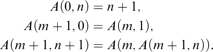 $$ \begin{align*} A(0,n) & = n+1,\\ A(m+1,0) & = A(m,1),\\ A(m+1,n+1) & = A(m,A(m+1,n)). \end{align*} $$
In 1993, Szasz [Reference Szasz16] proved that Ackermann’s function was not primitive recursive using a type theory based proof assistant called ALF.
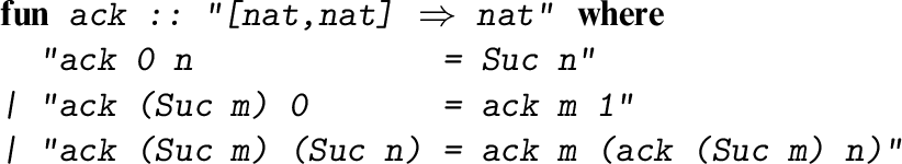
Isabelle/HOL [Reference Nipkow and Klein13, Reference Nipkow, Paulson and Wenzel14] is a proof assistant based on higher-order logic. Its underlying logic is much simpler than the type theories used in Coq for example. In particular, the notion of a recursive function is not primitive to higher-order logic but is derivable. We can introduce Ackermann’s function to Isabelle/HOL as shown below. The specification invokes internal machinery to generate a low-level definition and derive the claimed identities from it. Here Suc denotes the successor function for the natural numbers (type nat ).
It is easy to see that the recursion is well defined and terminating. In every recursive call, either the first or the second argument decreases by one, suggesting a termination ordering: the lexicographic combination of
 $<$
(on the natural numbers) for the two arguments.
$<$
(on the natural numbers) for the two arguments.
Nevertheless, it’s not straightforward to prove that Ackermann’s function belongs to the class of computable functions in a formal sense. Cutland [Reference Cutland6, pp. 46–47] devotes an entire page to the sketch of a construction to show that Ackermann’s function could be computed using a register machine, before remarking that “a sophisticated proof” is available as an application of more advanced results, presumably the recursion theorem. This raises the question of whether Ackermann’s function has some alternative definition that is easier to reason about, and in fact, iterative definitions exist. But then we must prove that the recursive and iterative definitions are equivalent.
The proof is done using the function definition facilities of Isabelle/HOL and is a good demonstration of their capabilities to the uninitiated. But first, we need to consider how function definitions are handled in Isabelle/HOL and how the later relates to symbolic logic.
2 Recursive function definitions in Isabelle/HOL
Isabelle’s higher-order logic is a form of Church’s simple type theory [Reference Church5]. As with Church, it is based on the typed
 $\lambda $
-calculus with function types (written
$\lambda $
-calculus with function types (written
 $\alpha \to \beta $
: Greek letters range over types) and a type of booleans (written
bool
). Again following Church, the axiom of choice is provided through Hilbert’s epsilon operator
$\alpha \to \beta $
: Greek letters range over types) and a type of booleans (written
bool
). Again following Church, the axiom of choice is provided through Hilbert’s epsilon operator
 $\epsilon x. \phi $
, denoting some a such that
$\epsilon x. \phi $
, denoting some a such that
 $\phi (a)$
if such exists and otherwise any value.
$\phi (a)$
if such exists and otherwise any value.
For Church, all types were built up from the booleans and a type of individuals, keeping types to the minimum required for consistency. Isabelle/HOL has a multiplicity of types in the spirit of functional programming, with numeric types
nat
,
int
,
real
, among countless others. Predicates have types of the form
![]() , but for reasons connected with performance, the distinct but equivalent type
, but for reasons connected with performance, the distinct but equivalent type
![]() is provided for sets of elements of type
is provided for sets of elements of type
 $\alpha $
.
$\alpha $
.
Gordon [Reference Gordon7] pioneered the use of simple type theory for verifying hardware. His first computer implementation, and the later HOL Light [Reference Harrison9], hardly deviate from Church. Constants can be introduced, but they are essentially abbreviations. The principles for defining new types do not stretch things much further: they allow the declaration of a new type corresponding to what Church would have called “a non-empty class given by a propositional function” (a predicate over an existing type). These principles, some criticisms of them and proposed alternatives are explored by Arthan [Reference Arthan2].
The idea of derivations schematic over types is already implicit in Church (“typical ambiguity”), and in most implementations is placed on a formal basis by including type variables in the calculus. Then all constructions involving types can be schematic, or polymorphic, allowing for example a family of types of the form
![]() , conventionally written in postfix notation. Refining the notion of polymorphism to allow classes of type variables associated with axioms—so-called axiomatic type classes—is a major extension to Church’s original conception, and has required a thoroughgoing analysis [Reference Kunčar and Popescu12]. However, those extensions are not relevant here, where we are only interested in finite sequences of integers.
, conventionally written in postfix notation. Refining the notion of polymorphism to allow classes of type variables associated with axioms—so-called axiomatic type classes—is a major extension to Church’s original conception, and has required a thoroughgoing analysis [Reference Kunčar and Popescu12]. However, those extensions are not relevant here, where we are only interested in finite sequences of integers.
There are a number of ways to realise a logical calculus on a computer. At one extreme, the implementer might choose a fast, unsafe language such as C and write arbitrarily complex code, implementing algorithms that have been shown to be sound with respect to the chosen calculus. Automatic theorem provers follow this approach. Most proof assistants, including Isabelle, take the opposite extreme and prioritise correctness. The implementer codes the axioms and inference rules of the calculus in something approaching their literal form: providing syntactic operations on types and terms while encapsulating the logical rules within a small, dedicated proof kernel. This LCF architecture [Reference Gordon8] requires a safe programming language so that the proof kernel—which has the exclusive right to declare a formula to be a theorem—can be protected from any bugs in the rest of the system.
Formal proofs are frequently colossal, so most proof assistants provide automation. In Isabelle, the auto proof method simplifies arithmetic expressions, expands functions when they are applied to suitable arguments and performs simple logical reasoning. Users can add automation to Isabelle by writing code for say a decision procedure, but such code (like auto itself) must lie outside the proof kernel and must reduce its proofs to basic inferences so that they can pass through the kernel. In this way, the LCF architecture eliminates the need to store the low-level proofs themselves, a vital space saving even in the era of 32 GB laptops.
Sophisticated principles for defining inductive sets, recursive functions with pattern matching and recursive types can be reduced to pure higher-order logic. In accordance with the LCF architecture, such definitions are translated into the necessary low-level form by Isabelle/HOL code that lies outside the proof kernel. This code defines basic constructions, from which it then proves desired facts, such as the function’s recursion equations.
In mathematics, a recursive function must always be shown to be well defined. Non-terminating recursion equations cannot be asserted unconditionally, since they could yield a contradiction: consider
 $f(m,n) = f(n,m)+1$
, which implies
$f(m,n) = f(n,m)+1$
, which implies
 $f(0,0) = f(0,0)+1$
. Isabelle/HOL’s function package, due to Krauss [Reference Krauss11], reduces recursive function definitions to inductively defined relations. A recursive function f is typically partial, so the package also defines its domain
$f(0,0) = f(0,0)+1$
. Isabelle/HOL’s function package, due to Krauss [Reference Krauss11], reduces recursive function definitions to inductively defined relations. A recursive function f is typically partial, so the package also defines its domain
 $D_f$
, the set of values for which f obeys its recursion equations.Footnote
1
$D_f$
, the set of values for which f obeys its recursion equations.Footnote
1
The idea of inductive definitions should be familiar, as when we say the set of theorems is inductively generated by the given axioms and inference rules. Formally, a set
 $I(\Phi )$
is inductively defined with respect to a collection
$I(\Phi )$
is inductively defined with respect to a collection
 $\Phi $
of rules provided it is closed under
$\Phi $
of rules provided it is closed under
 $\Phi $
and is the least such set [Reference Aczel1]. In higher-order logic,
$\Phi $
and is the least such set [Reference Aczel1]. In higher-order logic,
 $I(\Phi )$
can be defined as the intersection of all sets closed under a collection of rules:
$I(\Phi )$
can be defined as the intersection of all sets closed under a collection of rules:
 $I(\Phi ) = \bigcap \{ A \mid A \text { is } \Phi \text {-closed}\}$
. The minimality of
$I(\Phi ) = \bigcap \{ A \mid A \text { is } \Phi \text {-closed}\}$
. The minimality of
 $I(\Phi )$
, namely that
$I(\Phi )$
, namely that
 $I(\Phi )\subseteq A$
if A is
$I(\Phi )\subseteq A$
if A is
 $\Phi $
-closed, gives rise to a familiar principle for proof by induction. Even Church [Reference Church5] included a construction of the natural numbers. Isabelle provides a package to automate inductive definitions [Reference Paulson15].
$\Phi $
-closed, gives rise to a familiar principle for proof by induction. Even Church [Reference Church5] included a construction of the natural numbers. Isabelle provides a package to automate inductive definitions [Reference Paulson15].
Krauss’ function package [Reference Krauss11] includes many refinements so as to handle straightforward function definitions—like the one shown in the introduction—without fuss. Definitions go through several stages of processing. The specification of a function f is examined, following the recursive calls, to yield inductive definitions of its graph
 $G_f$
and domain
$G_f$
and domain
 $D_f$
. The package proves that
$D_f$
. The package proves that
 $G_f$
corresponds to a well-defined function on its domain. It is then possible to define f formally in terms of
$G_f$
corresponds to a well-defined function on its domain. It is then possible to define f formally in terms of
 $G_f$
and to derive the desired recursion equations, each conditional on the function being applied within its domain. The refinements alluded to above include dealing with pattern matching and handling easy cases of termination, where the domain can be hidden. But in the example considered below, we are forced to prove termination ourselves through a series of inductions.
$G_f$
and to derive the desired recursion equations, each conditional on the function being applied within its domain. The refinements alluded to above include dealing with pattern matching and handling easy cases of termination, where the domain can be hidden. But in the example considered below, we are forced to prove termination ourselves through a series of inductions.
For a simple example [Reference Krauss11, Section 3.5.4], consider the everywhere undefined function given by
 $U(x) = U(x)+1$
. The graph is defined inductively by the rule
$U(x) = U(x)+1$
. The graph is defined inductively by the rule
 $$ \begin{align*} (x, h(x)) \in G_U \Longrightarrow (x, h(x)+1) \in G_U.\end{align*} $$
Similarly, the domain is defined inductively by the rule
 $$ \begin{align*} x \in D_U \Longrightarrow x \in D_U.\end{align*} $$
It should be obvious that
 $G_U$
and
$G_U$
and
 $D_U$
are both empty and that the evaluation rule
$D_U$
are both empty and that the evaluation rule
 $x \in D_U \Longrightarrow U(x) = U(x)+1$
holds vacuously. But we can also see how less trivial examples might be handled, as in the extended example that follows.
$x \in D_U \Longrightarrow U(x) = U(x)+1$
holds vacuously. But we can also see how less trivial examples might be handled, as in the extended example that follows.
3 An iterative version of Ackermann’s function
A list is a possibly empty finite sequence, written
 $[x_1,\ldots ,x_n]$
or equivalently
$[x_1,\ldots ,x_n]$
or equivalently
 $x_1\mathbin {\#} \cdots \mathbin {\#} x_n\mathbin {\#} []$
. Note that
$x_1\mathbin {\#} \cdots \mathbin {\#} x_n\mathbin {\#} []$
. Note that
 $\mathbin {\#}$
is the operation that extends a list from the front with a new element. We can write an iterative definition of A in terms of the following recursion on lists:
$\mathbin {\#}$
is the operation that extends a list from the front with a new element. We can write an iterative definition of A in terms of the following recursion on lists:
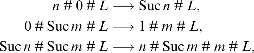 $$ \begin{align*} n\mathbin{\#} 0\mathbin{\#} L &\longrightarrow \operatorname{\mathrm{Suc}} n \mathbin{\#} L,\\ 0\mathbin{\#} \operatorname{\mathrm{Suc}} m\mathbin{\#} L &\longrightarrow 1\mathbin{\#} m \mathbin{\#} L,\\ \operatorname{\mathrm{Suc}} n\mathbin{\#} \operatorname{\mathrm{Suc}} m\mathbin{\#} L &\longrightarrow n\mathbin{\#} \operatorname{\mathrm{Suc}} m\mathbin{\#} m \mathbin{\#} L, \end{align*} $$
the idea being to replace the recursive calls by a stack. We intend that a computation starting with a two-element list will yield the corresponding value of Ackermann’s function:
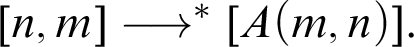 $$ \begin{align*} [n,m] \longrightarrow^* [A(m,n)]. \end{align*} $$
An execution trace for
 $A(2,3)$
looks like this:
$A(2,3)$
looks like this:
3 2
2 2 1
1 2 1 1
0 2 1 1 1
1 1 1 1 1
0 1 0 1 1 1
1 0 0 1 1 1
2 0 1 1 1
3 1 1 1
2 1 0 1 1
1 1 0 0 1 1
0 1 0 0 0 1 1
1 0 0 0 0 1 1
2 0 0 0 1 1
3 0 0 1 1
4 0 1 1
5 1 1
4 1 0 1
3 1 0 0 1
2 1 0 0 0 1
1 1 0 0 0 0 1
0 1 0 0 0 0 0 1
1 0 0 0 0 0 0 1
2 0 0 0 0 0 1
3 0 0 0 0 1
4 0 0 0 1
5 0 0 1
6 0 1
7 1
6 1 0
5 1 0 0
4 1 0 0 0
3 1 0 0 0 0
2 1 0 0 0 0 0
1 1 0 0 0 0 0 0
0 1 0 0 0 0 0 0 0
1 0 0 0 0 0 0 0 0
2 0 0 0 0 0 0 0
3 0 0 0 0 0 0
4 0 0 0 0 0
5 0 0 0 0
6 0 0 0
7 0 0
8 0
9
We can regard these three reductions as constituting a term rewriting system [Reference Baader and Nipkow4], subject to the proviso that they can only rewrite at the front of the list. Equivalently, each rewrite rule can be imagined as beginning with an anchor symbol, say
 $\Box $
:
$\Box $
:
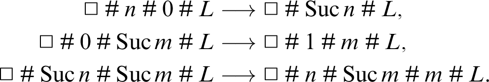 $$ \begin{align*} \Box \mathbin{\#} n\mathbin{\#} 0\mathbin{\#} L &\longrightarrow \Box \mathbin{\#} \operatorname{\mathrm{Suc}} n \mathbin{\#} L,\\ \Box \mathbin{\#} 0\mathbin{\#} \operatorname{\mathrm{Suc}} m\mathbin{\#} L &\longrightarrow \Box \mathbin{\#} 1\mathbin{\#} m \mathbin{\#} L,\\ \Box \mathbin{\#} \operatorname{\mathrm{Suc}} n\mathbin{\#} \operatorname{\mathrm{Suc}} m\mathbin{\#} L &\longrightarrow \Box \mathbin{\#} n\mathbin{\#} \operatorname{\mathrm{Suc}} m\mathbin{\#} m \mathbin{\#} L. \end{align*} $$
A term rewriting system is a model of computation in itself. But termination isn’t obvious here. In the first rewrite rule above, the head of the list gets bigger while the list gets shorter, suggesting that the length of the list should be the primary termination criterion. But in the third rewrite rule, the list gets longer. One might imagine a more sophisticated approach to termination based on multisets or ordinals; these however could lead nowhere because the second rewrite allows
 $0\mathbin {\#} 1\mathbin {\#} L \longrightarrow 1\mathbin {\#} 0 \mathbin {\#} L$
and often these approaches ignore the order of the list elements.
$0\mathbin {\#} 1\mathbin {\#} L \longrightarrow 1\mathbin {\#} 0 \mathbin {\#} L$
and often these approaches ignore the order of the list elements.
Although some natural termination ordering might be imagined to exist,Footnote 2 this system is an excellent way to demonstrate another approach to proving termination: by explicit reasoning about the domain of definition. It is easy, using Isabelle/HOL’s function definition package [Reference Krauss11].
4 The iterative version in Isabelle/HOL
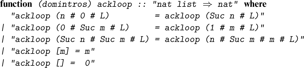
We would like to formalise the iterative computation described above as a recursive function, but we don’t know that it terminates. Isabelle allows the following form, with the keyword domintros , indicating that we wish to defer the termination proof and reason explicitly about the function’s domain. Our goal is to show that the set is universal (for its type).
The domain, which is called ackloop_dom , is generated according to the recursive calls. It is defined inductively to satisfy the following propertiesFootnote 3 :
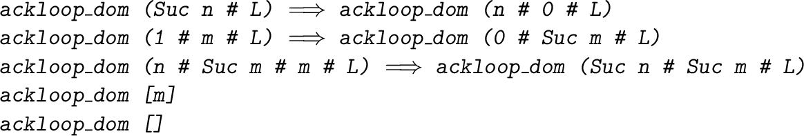
For example, the first line states that if ackloop terminates for Suc n # L then it will also terminate for n # 0 # L , as we can see for ourselves by looking at the first line of ackloop . The second and third lines similarly follow the recursion. The last two lines are unconditional because there is no recursion.
It’s obvious that ackloop_dom holds for all lists shorter than two elements. Its properties surely allow us to prove instances for longer lists (thereby establishing termination of ackloop for those lists), but how? At closer examination, remembering that ackloop represents the recursion of Ackermann’s function, we might come up with the following lemma:
This could be the solution, since it implies that
ackloop
terminates on the list
 $n\mathbin {\#} m\mathbin {\#} L$
provided it terminates on
$n\mathbin {\#} m\mathbin {\#} L$
provided it terminates on
 $A(m,n)\mathbin {\#} L$
, a shorter list. And indeed it can easily be proved by mathematical induction on m followed by a further induction on n. If
$A(m,n)\mathbin {\#} L$
, a shorter list. And indeed it can easily be proved by mathematical induction on m followed by a further induction on n. If
 $m=0$
then it simplifies to the first
ackloop_dom
property:
$m=0$
then it simplifies to the first
ackloop_dom
property:
In the
 $\operatorname {\mathrm {Suc}} m$
case, after the induction on n, the
$\operatorname {\mathrm {Suc}} m$
case, after the induction on n, the
 $n=0$
case simplifies to
$n=0$
case simplifies to
but from
ackloop_dom (ack m 1 # L)
the induction hypothesis yields
ackloop_dom (1 # m # L)
, from which we obtain
ackloop_dom (0 # Suc m # L)
by the second
ackloop_dom
property. The
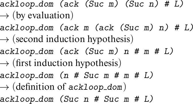
 $\operatorname {\mathrm {Suc}} n$
case is also straightforward
$\operatorname {\mathrm {Suc}} n$
case is also straightforward
It needs the third ackloop_dom property and both induction hypotheses. The details are left as an exercise.
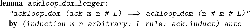
In Isabelle, the lemma proved above can be proved in one line, thanks to a special induction rule:
ack.induct
. The definition of a function f in Isabelle automatically yields an induction rule customised to the recursive calls, derived from the inductive definition of
 $G_f$
. For
ack
, it allows us to prove any formula
$G_f$
. For
ack
, it allows us to prove any formula
 $P(x,y)$
from the three premises
$P(x,y)$
from the three premises
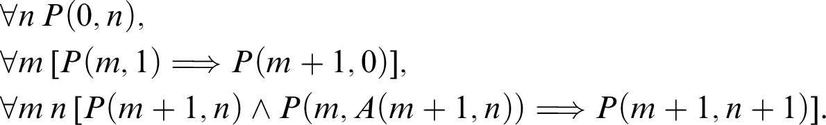 $$ \begin{align*} & \forall n\,P(0,n),\\ & \forall m\, [P(m,1) \Longrightarrow P (m+1, 0)],\\ & \forall m\,n\, [P (m+1, n) \land P(m, A(m+1,n)) \Longrightarrow P (m+1,n+1)]. \end{align*} $$
Using this induction rule, our lemma follows immediately by simple rewriting:
Let’s examine this proof. In the induction,
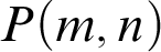 $P(m,n)$
is the formula
$P(m,n)$
is the formula
In most difficult case,
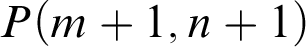 $P (m+1,n+1)$
, the left-hand side is
$P (m+1,n+1)$
, the left-hand side is
And this is the right-hand side of
 $P (m+1,n+1)$
.
$P (m+1,n+1)$
.
It must be stressed that when typing in the Isabelle proof shown above for lemma ackloop_dom_longer , I did not have this or any derivation in mind. Experienced users know that properties of a recursive function f often have extremely simple proofs by induction on f.induct followed by auto (basic automation), so they type the corresponding Isabelle commands without thinking. We are gradually managing to shift the burden of thinking to the computer.
5 Completing the proof
Given the lemma just proved, it’s clear that every list L satisfies
ackloop_dom
by induction on the length l of L: if
 $l<2$
then the result is immediate, and otherwise it has the form
$l<2$
then the result is immediate, and otherwise it has the form
 $n\mathbin {\#} m \mathbin {\#} L'$
, which the lemma reduces to
$n\mathbin {\#} m \mathbin {\#} L'$
, which the lemma reduces to
 $A(m,n) \mathbin {\#} L'$
and we are finished by the induction hypothesis.
$A(m,n) \mathbin {\#} L'$
and we are finished by the induction hypothesis.
A slicker proof turns out to be possible. Consider what
ackloop
is actually designed to do: to replace the first two list elements, n and m, by
 $A(m,n)$
. The following function codifies this point.
$A(m,n)$
. The following function codifies this point.
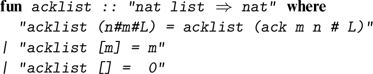
As mentioned above, recursive function definitions automatically provide us with a customised induction rule. In the case of acklist , it performs exactly the case analysis sketched at the top of this section. So this proof is also a single induction followed by automation. Note the reference to ackloop_dom_longer , the lemma proved above.

It is possible to reconstruct the details of this proof by running it interactively, as was done in the previous section. But perhaps it is better to repeat that these Isabelle commands were typed without having any detailed proof in mind but simply with the knowledge that they were likely to be successful.
Now that ackloop_dom is known to hold for arbitrary L , we can issue a command to inform Isabelle that ackloop is a total function satisfying unconditional recursion equations. We mention the termination result just proved.
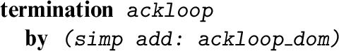
The equivalence between ackloop and acklist is another one-line induction proof. The induction rule for ackloop considers the five cases of that function’s definition, which—as we have seen twice before—are all proved automatically.

The equivalence between the iterative and recursive definitions of Ackermann’s function is now immediate.
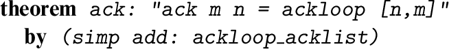
We had a function that obviously terminated but was not obviously computable (in the sense of Turing machines and similar formal models) and another function that was obviously computable but not obviously terminating. The proof of the termination of the latter has led immediately to a proof of equivalence with the former.
Anybody who has used a proof assistant knows that machine proofs are generally many times longer than typical mathematical exposition. Our example here is a rare exception.
Acknowledgements
This work was supported by the ERC Advanced Grant ALEXANDRIA (Project GA 742178). René Thiemann investigated the termination of the corresponding rewrite systems. I am grateful to the editor, Peter Dybjer, and the referee for their comments.


 Open access