


1 Introduction
Let p be a prime and consider the modular curve $Y_0(p)=\Gamma _0(p)\backslash \mathbb {H}$
of level p equipped with the hyperbolic line element
$Y_0(p)=\Gamma _0(p)\backslash \mathbb {H}$
of level p equipped with the hyperbolic line element $|dz|/y$
and volume element
$|dz|/y$
and volume element $dxdy/y^2$
, where
$dxdy/y^2$
, where $\mathbb {H}=\{z=x+iy\in \mathbb {C}: y>0\}$
is the upper half-plane and
$\mathbb {H}=\{z=x+iy\in \mathbb {C}: y>0\}$
is the upper half-plane and $\Gamma _0(p)\leq \mathrm {PSL}_2(\mathbb {Z})$
is the level p Hecke congruence groupFootnote
1
acting on
$\Gamma _0(p)\leq \mathrm {PSL}_2(\mathbb {Z})$
is the level p Hecke congruence groupFootnote
1
acting on $\mathbb {H}$
by linear fractional transformations. Given a real quadratic field K of discriminant
$\mathbb {H}$
by linear fractional transformations. Given a real quadratic field K of discriminant $d_K>0$
such that p splits in K, one can associate to an element
$d_K>0$
such that p splits in K, one can associate to an element $A\in \mathrm {Cl}_K^+$
of the narrow class group of K an oriented closed geodesic
$A\in \mathrm {Cl}_K^+$
of the narrow class group of K an oriented closed geodesic $\mathcal {C}_{A}(p)$
on
$\mathcal {C}_{A}(p)$
on $Y_0(p)$
(see Section 3.1 for details). In a celebrated paper [Reference DukeDuk88], Duke proved that the geodesics
$Y_0(p)$
(see Section 3.1 for details). In a celebrated paper [Reference DukeDuk88], Duke proved that the geodesics $\{\mathcal {C}_{A}(p)\subset Y_0(p): A\in \mathrm {Cl}_K^+\}$
equidistribute with respect to hyperbolic measure as
$\{\mathcal {C}_{A}(p)\subset Y_0(p): A\in \mathrm {Cl}_K^+\}$
equidistribute with respect to hyperbolic measure as $d_K$
tends to infinity, meaning that
$d_K$
tends to infinity, meaning that
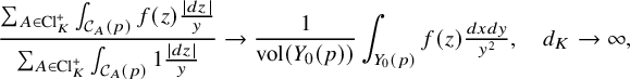 $$ \begin{align} \frac{\sum_{A\in \mathrm{Cl}_K^+} \int_{\mathcal{C}_{A}(p)} f(z)\tfrac{|dz|}{y}}{\sum_{A\in \mathrm{Cl}_K^+} \int_{\mathcal{C}_{A}(p)} 1 \tfrac{|dz|}{y}}\rightarrow \frac{1}{\mathrm{vol}(Y_0(p))}\int_{Y_0(p)} f(z)\tfrac{dxdy}{y^2}, \quad d_K\rightarrow \infty, \end{align} $$
for $f:Y_0(p)\rightarrow \mathbb {C}$
smooth of compact support (for further results, see [Reference Einsiedler, Lindenstrauss, Michel and VenkateshELMV12], [Reference Michel and VenkateshMV06] and the reference therein). In this paper, we study the homological behavior of the oriented closed geodesics – that is, the map
$f:Y_0(p)\rightarrow \mathbb {C}$
smooth of compact support (for further results, see [Reference Einsiedler, Lindenstrauss, Michel and VenkateshELMV12], [Reference Michel and VenkateshMV06] and the reference therein). In this paper, we study the homological behavior of the oriented closed geodesics – that is, the map
 $$ \begin{align} \mathrm{Cl}_K^+\rightarrow H_1(Y_0(p),\mathbb{Z}), \quad A\mapsto [\mathcal{C}_{A}(p)]:=\text{class of }\mathcal{C}_{A}(p),\end{align} $$
from the narrow class group to the integral homology of $Y_0(p)$
(which one can identity with the abelinization of
$Y_0(p)$
(which one can identity with the abelinization of $\Gamma _0(p)$
modulo torsion) as
$\Gamma _0(p)$
modulo torsion) as $d_K \rightarrow \infty $
. Our result can be stated as saying that the classes concentrate around the Eisenstein line. This is a real quadratic analogue of the equidistribution of supersingular reduction of CM elliptic curves as in [Reference MichelMic04] (see Section 2). We also study the level aspect (analogue of [Reference Liu, Masri and YoungLMY15]) leading to a homological version of the sup norm problem (see Section 6) which might be of independent interest (for another application, consult [Reference Humphries and NordentoftHN22]). We also present applications of our distribution results – one group theoretic and another concerning nonvanishing of cycle integrals of modular forms (see Section 1.2). Finally, we refer to Section 1.3 and Remark 1.9 below for geometric interpretations of our results.
$d_K \rightarrow \infty $
. Our result can be stated as saying that the classes concentrate around the Eisenstein line. This is a real quadratic analogue of the equidistribution of supersingular reduction of CM elliptic curves as in [Reference MichelMic04] (see Section 2). We also study the level aspect (analogue of [Reference Liu, Masri and YoungLMY15]) leading to a homological version of the sup norm problem (see Section 6) which might be of independent interest (for another application, consult [Reference Humphries and NordentoftHN22]). We also present applications of our distribution results – one group theoretic and another concerning nonvanishing of cycle integrals of modular forms (see Section 1.2). Finally, we refer to Section 1.3 and Remark 1.9 below for geometric interpretations of our results.
1.1 Statement of results
Let p be prime and let g denote the genus of the (noncompact) Riemann surface $Y_0(p)$
satisfying
$Y_0(p)$
satisfying $g=\tfrac {p}{12}+O(1)$
. The integral homology
$g=\tfrac {p}{12}+O(1)$
. The integral homology
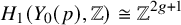 $$ \begin{align*} H_1(Y_0(p),\mathbb{Z})\cong \mathbb{Z}^{2g+1} \end{align*} $$
sits as a lattice inside the real homology
 $$ \begin{align} V_p:=H_1(Y_0(p),\mathbb{R})\cong \Gamma_0(p)^{\mathrm{ab}}\otimes \mathbb{R} \cong \mathbb{R}^{2g+1}. \end{align} $$
We will be interested in how elements of $V_p$
distribute when projected to the
$V_p$
distribute when projected to the $2g$
-sphere, by which we mean the map
$2g$
-sphere, by which we mean the map
 $$ \begin{align} V_p-\{0\}\twoheadrightarrow\mathbf{S}(V_p):=(V_p-\{0\})/\mathbb{R}_{>0} , \quad v\mapsto \overline{v}, \end{align} $$
where we endow $\mathbf {S}(V_p)$
with the quotient topology of the Euclidean topology of
$\mathbf {S}(V_p)$
with the quotient topology of the Euclidean topology of $V_p$
. We define the Eisenstein class
$V_p$
. We define the Eisenstein class
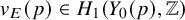 $$ \begin{align} v_{E}(p)\in H_1(Y_0(p),\mathbb{Z}) \end{align} $$
as the homology class of a simple loop going once around the cusp at $\infty $
with positive orientation (which corresponds to the image of the matrix
$\infty $
with positive orientation (which corresponds to the image of the matrix
![]() in
in $\Gamma _0(p)^{\mathrm {ab}}$
using the identification (1.3)). This is indeed a Hecke eigenclass with the same eigenvalues as the weight
$\Gamma _0(p)^{\mathrm {ab}}$
using the identification (1.3)). This is indeed a Hecke eigenclass with the same eigenvalues as the weight $2$
Eisenstein series, as we will see in Section 3.2.1. Our first main result is the following.
$2$
Eisenstein series, as we will see in Section 3.2.1. Our first main result is the following.
Theorem 1.1. Let p be a prime and consider a real quadratic field K of discriminant $d_K $
such that p splits in K with
$d_K $
such that p splits in K with $p\mathcal {O}_K=\mathfrak {p}_1\mathfrak {p}_2$
. Consider a subgroup
$p\mathcal {O}_K=\mathfrak {p}_1\mathfrak {p}_2$
. Consider a subgroup $H\leq \mathrm {Cl}_K^+$
such that
$H\leq \mathrm {Cl}_K^+$
such that $\mathfrak {p}_1 \notin H$
and
$\mathfrak {p}_1 \notin H$
and $(\sqrt {d_K})\notin H$
. Then as
$(\sqrt {d_K})\notin H$
. Then as $d_K \rightarrow \infty $
, the classes of the closed geodesics associated to H concentrate around the line generated by the Eisenstein element, meaning that
$d_K \rightarrow \infty $
, the classes of the closed geodesics associated to H concentrate around the line generated by the Eisenstein element, meaning that
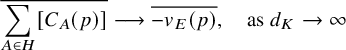 $$ \begin{align} \overline{\sum_{A\in H} [C_A(p)]} \longrightarrow \overline{- v_{E}(p)} , \quad \text{as }d_K \rightarrow \infty \end{align} $$
in the quotient topology of $\mathbf {S}(V_p)$
.
$\mathbf {S}(V_p)$
.
This is the real quadratic analogue of a distribution result due to Michel [Reference MichelMic04] (see also [Reference Elkies, Ono and YangEOY05], [Reference YangYan08], [Reference KaneKan09], [Reference Liu, Masri and YoungLMY15] and [Reference Aka, Luethi, Michel and WieserALMW22]) concerning the map
 $$ \begin{align} \mathrm{Cl}_K\rightarrow \mathcal{E\ell\ell}^{ss}(\mathbb{F}_{p^2}) \end{align} $$
from the class group of an imaginary quadratic field K (in which p is inert) to the isomorphism classes of supersingular elliptic curves defined over $\mathbb {F}_{p^2}$
(or equivalently over
$\mathbb {F}_{p^2}$
(or equivalently over $\overline {\mathbb {F}_p}$
). We refer to Section 2 for a more elaborate explanation of the analogy between the two cases. We note also that our results can be phrased as a weak convergence statement (see Theorem 5.1) which resembles (1.1). Another useful analogue to have in mind is the distribution of lattice points on the unit sphere
$\overline {\mathbb {F}_p}$
). We refer to Section 2 for a more elaborate explanation of the analogy between the two cases. We note also that our results can be phrased as a weak convergence statement (see Theorem 5.1) which resembles (1.1). Another useful analogue to have in mind is the distribution of lattice points on the unit sphere $S^2\subset \mathbb {R}^3$
[Reference DukeDuk88]:
$S^2\subset \mathbb {R}^3$
[Reference DukeDuk88]:
 $$ \begin{align*}\frac{1}{\sqrt{d}}\{(a,b,c)\in \mathbb{Z}^3: a^2+b^2+c^2=d\}\subset S^2,\end{align*} $$
as $d\rightarrow \infty $
(which is the basic case of Linnik’s Problem; see [Reference Michel and VenkateshMV06]); in both cases, one rescales the points to get a convergence of measures to, respectively, the Haar measure and the point measure at (minus) the Eisenstein element. We have the following useful corollary. In Section 1.3 below, we will use this to explain the geometric content of our result.
$d\rightarrow \infty $
(which is the basic case of Linnik’s Problem; see [Reference Michel and VenkateshMV06]); in both cases, one rescales the points to get a convergence of measures to, respectively, the Haar measure and the point measure at (minus) the Eisenstein element. We have the following useful corollary. In Section 1.3 below, we will use this to explain the geometric content of our result.
Corollary 1.2. Let K and $H\leq \mathrm {Cl}_K^+$
be as in Theorem 1.1 and consider a basis B of
$H\leq \mathrm {Cl}_K^+$
be as in Theorem 1.1 and consider a basis B of $ V_p$
containing
$ V_p$
containing $v_{E}(p)$
. Then for
$v_{E}(p)$
. Then for $d_K$
sufficiently large, the
$d_K$
sufficiently large, the $v_{E}(p)$
-coordinate of the vector
$v_{E}(p)$
-coordinate of the vector
 $$ \begin{align*}\sum_{A\in H} [\mathcal{C}_{A}(p)]\in V_p\end{align*} $$
in the basis B has strictly maximal absolute value among all coordinates (and in particular is nonzero).
Remark 1.3. The conditions on the level and discriminant in the theorems above are necessary. If either $p\mathcal {O}_K=\mathfrak {p}_1\mathfrak {p}_2$
with
$p\mathcal {O}_K=\mathfrak {p}_1\mathfrak {p}_2$
with $\mathfrak {p}_1 \in (\mathrm {Cl}_K^+)^2$
or
$\mathfrak {p}_1 \in (\mathrm {Cl}_K^+)^2$
or $(\sqrt {d_K})\in H$
, then there is a basis for
$(\sqrt {d_K})\in H$
, then there is a basis for $V_p$
(the Hecke basis) such that the
$V_p$
(the Hecke basis) such that the $v_{E}(p)$
-coordinate of
$v_{E}(p)$
-coordinate of
 $$ \begin{align*}\sum_{A\in (\mathrm{Cl}_K^+)^2} [\mathcal{C}_{A}(p)]\end{align*} $$
is zero. In Section 3.1, we construct for each p an infinite family of real quadratic fields K that satisfy the conditions in Theorem 1.1. It is unclear whether the statement should be true for any genus.
Remark 1.4. The restriction to prime level ensures that there are no old forms and also that there is a unique Eisenstein class in the (co)homology. The main steps in the proofs should, however, work for general (square-free) level, but the statements would have to be modified accordingly.
1.1.1 Varying the level
Our second result is concerned with the level aspect in the sense that we will obtain a distribution statement uniform in p. Notice, first of all, that for $v_0,v_1, \ldots \in V_p-\{0\} $
, the convergence
$v_0,v_1, \ldots \in V_p-\{0\} $
, the convergence
 $$ \begin{align*}\overline{v_n}\longrightarrow \overline{v_0}\in \mathbf{S}(V_p)\text{ as } n\rightarrow \infty\end{align*} $$
is equivalent to
 $$ \begin{align} \left| \left|\frac{v_n}{|\!|v_n|\!|}-\frac{v_0}{|\!|v_0|\!|}\right| \right| \rightarrow 0\text{ as } n\rightarrow \infty\end{align} $$
for any (fixed) norm $|\!|\cdot |\!|$
of
$|\!|\cdot |\!|$
of $V_p$
. A natural question is to ask for bounds for the left-hand side of (1.8) uniform in
$V_p$
. A natural question is to ask for bounds for the left-hand side of (1.8) uniform in $d_K$
and p for certain specific norms of
$d_K$
and p for certain specific norms of $V_p$
. A basis B for
$V_p$
. A basis B for $H_1(Y_0(p),\mathbb {R})$
defines an isomorphism of vector spaces
$H_1(Y_0(p),\mathbb {R})$
defines an isomorphism of vector spaces $V_p\cong \mathbb {R}^{2g+1}$
(by mapping B to the standard basis of
$V_p\cong \mathbb {R}^{2g+1}$
(by mapping B to the standard basis of $\mathbb {R}^{2g+1}$
), and by pulling back the
$\mathbb {R}^{2g+1}$
), and by pulling back the $L^r$
-norm for
$L^r$
-norm for $1\leq r \leq \infty $
, we obtain a norm on
$1\leq r \leq \infty $
, we obtain a norm on $V_p$
which we denote by
$V_p$
which we denote by $|\!|\cdot |\!|_{B,r}$
(see (7.3) for details). We notice that one can choose a sequence of bases for each p such that the convergence in (1.8) (with say
$|\!|\cdot |\!|_{B,r}$
(see (7.3) for details). We notice that one can choose a sequence of bases for each p such that the convergence in (1.8) (with say $r=1$
) is arbitrarily slow in p. This is parallel to the case of the distribution of CM points on modular curves in the level aspect as considered in [Reference Liu, Masri and YoungLMY13]; here, one has to consider ‘compatible’ test functions as the level varies. Similarly, we will consider certain ‘compatible’ bases of
$r=1$
) is arbitrarily slow in p. This is parallel to the case of the distribution of CM points on modular curves in the level aspect as considered in [Reference Liu, Masri and YoungLMY13]; here, one has to consider ‘compatible’ test functions as the level varies. Similarly, we will consider certain ‘compatible’ bases of $H_1(Y_0(p),\mathbb {R})$
. To define these, we recall (see Section 4.2) that the following matrices generate
$H_1(Y_0(p),\mathbb {R})$
. To define these, we recall (see Section 4.2) that the following matrices generate $\Gamma _0(p)$
;
$\Gamma _0(p)$
;
where $0< a^\ast <p$
is such that
$0< a^\ast <p$
is such that $aa^{\ast } \equiv -1 \ \mathrm {mod}\ p$
. We say that a basis B of
$aa^{\ast } \equiv -1 \ \mathrm {mod}\ p$
. We say that a basis B of $H_1(Y_0(p), \mathbb {R})$
is a basic basis of level p if it consists of homology classes containing the oriented geodesic connecting
$H_1(Y_0(p), \mathbb {R})$
is a basic basis of level p if it consists of homology classes containing the oriented geodesic connecting $i\in \mathbb {H}$
and
$i\in \mathbb {H}$
and $\sigma i\in \mathbb {H}$
for some
$\sigma i\in \mathbb {H}$
for some $\sigma \in \mathcal {S}(p)$
. We think of these bases as analogues of the sets
$\sigma \in \mathcal {S}(p)$
. We think of these bases as analogues of the sets $\mathcal {E\ell \ell }^{ss}(\mathbb {F}_{p^2})$
considered in the imaginary quadratic case (1.7) (see Section 2). Our second main result is the following.
$\mathcal {E\ell \ell }^{ss}(\mathbb {F}_{p^2})$
considered in the imaginary quadratic case (1.7) (see Section 2). Our second main result is the following.
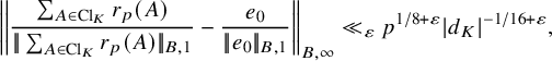
Theorem 1.5. Let p be prime and ${B}$
a basic basis of level p with associated norm
${B}$
a basic basis of level p with associated norm $|\!|\cdot |\!|_{{B},\infty }$
(note that
$|\!|\cdot |\!|_{{B},\infty }$
(note that $|\!|v_{E}(p)|\!|_{B,\infty }=1$
). Let K be a real quadratic field of discriminant
$|\!|v_{E}(p)|\!|_{B,\infty }=1$
). Let K be a real quadratic field of discriminant $d_K $
with no unit of norm
$d_K $
with no unit of norm $-1$
such that p splits in K with
$-1$
such that p splits in K with $p\mathcal {O}_K=\mathfrak {p}_1\mathfrak {p}_2$
and
$p\mathcal {O}_K=\mathfrak {p}_1\mathfrak {p}_2$
and $\mathfrak {p}_1\notin (\mathrm {Cl}^+_K)^2$
. Then we have
$\mathfrak {p}_1\notin (\mathrm {Cl}^+_K)^2$
. Then we have
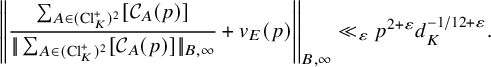 $$ \begin{align} \left| \left|\frac{\sum_{A\in (\mathrm{Cl}^+_K)^2} [\mathcal{C}_{A}(p)]}{|\!|\sum_{A\in (\mathrm{Cl}^+_K)^2} [\mathcal{C}_{A}(p)]|\!|_{B,\infty}}+v_{E}(p)\right|\right|_{B,\infty} \ll_{\varepsilon} p^{2+\varepsilon} d_K^{-1/12+\varepsilon}. \end{align} $$
As above, we get the following corollary.
Corollary 1.6. Let p and K be as above and consider a basic basis ${B}\subset V_p$
of level p containing
${B}\subset V_p$
of level p containing $v_{E}(p)$
. Then for
$v_{E}(p)$
. Then for $d_K\gg _\varepsilon p^{24+\varepsilon }$
, the
$d_K\gg _\varepsilon p^{24+\varepsilon }$
, the $v_{E}(p)$
-coordinate of the vector
$v_{E}(p)$
-coordinate of the vector
 $$ \begin{align*}\sum_{A\in (\mathrm{Cl}_K^+)^2} [\mathcal{C}_{A}(p)]\in V_p\end{align*} $$
in the basis ${B}$
has strictly maximal absolute value among all coordinates (and in particular is nonzero).
${B}$
has strictly maximal absolute value among all coordinates (and in particular is nonzero).
The above result has a very close analogue in the imaginary quadratic case as worked out by Liu–Masri–Young [Reference Liu, Masri and YoungLMY15], who studied a level p version of the equidistribution of the map (1.7). One can identify the finite set $\mathcal {E\ell \ell }^{ss}(\mathbb {F}_{p^2})=\{e_1,\ldots , e_n\}$
with the connected components of a certain conic curve
$\mathcal {E\ell \ell }^{ss}(\mathbb {F}_{p^2})=\{e_1,\ldots , e_n\}$
with the connected components of a certain conic curve $X^{p,\infty }$
defined from the quaternion algebra over
$X^{p,\infty }$
defined from the quaternion algebra over $\mathbb {Q}$
ramified at p and
$\mathbb {Q}$
ramified at p and $\infty $
. Thus,
$\infty $
. Thus, $\{e_1,\ldots , e_n\}$
defines a basis for the
$\{e_1,\ldots , e_n\}$
defines a basis for the $0$
-th homology group
$0$
-th homology group $H_0(X^{p,\infty },\mathbb {Z})$
. In this language, the results of [Reference Liu, Masri and YoungLMY15] can be phrased exactly as (1.10) (see (2.5)). We will develop this analogy in greater detail in Section 2.
$H_0(X^{p,\infty },\mathbb {Z})$
. In this language, the results of [Reference Liu, Masri and YoungLMY15] can be phrased exactly as (1.10) (see (2.5)). We will develop this analogy in greater detail in Section 2.
1.2 Applications
We will now present some applications of our results; one is group theoretic and the other has to do with nonvanishing of cycle integrals of modular forms.
Consider a prime $p\equiv -1 \ \mathrm {mod}\ 12$
(for simplicity) and put
$p\equiv -1 \ \mathrm {mod}\ 12$
(for simplicity) and put $n=\frac {p+1}{3}$
. Then
$n=\frac {p+1}{3}$
. Then $\Gamma _0(p)$
considered as a subgroup of
$\Gamma _0(p)$
considered as a subgroup of $\mathrm {PSL}_2(\mathbb {Z})$
is torsion-free with
$\mathrm {PSL}_2(\mathbb {Z})$
is torsion-free with $\Gamma _0(p)^{\mathrm {ab}}\cong \mathbb {Z}^{n/2+1}$
, and thus we know by the Kurosh subgroup theorem that
$\Gamma _0(p)^{\mathrm {ab}}\cong \mathbb {Z}^{n/2+1}$
, and thus we know by the Kurosh subgroup theorem that $\Gamma _0(p)$
is a free group on
$\Gamma _0(p)$
is a free group on $n/2+1$
generators (being a subgroup of
$n/2+1$
generators (being a subgroup of $\mathrm {PSL}_2(\mathbb {Z})\cong \mathbb {Z}/2\mathbb {Z} \ast \mathbb {Z}/3\mathbb {Z} $
). Let
$\mathrm {PSL}_2(\mathbb {Z})\cong \mathbb {Z}/2\mathbb {Z} \ast \mathbb {Z}/3\mathbb {Z} $
). Let
 $$ \begin{align*}\frac{0}{1}=\frac{a_{0}}{b_{0}}<\frac{a_1}{b_1}<\ldots<\frac{a_{n-1}}{b_{n-1}}< \frac{a_{n}}{b_{n}}=\frac{1}{1}\end{align*} $$
be a Farey symbol of level p in the terminology of Kulkarni [Reference KulkarniKul91], meaning that $a_i/b_i$
are reduced fractions such that
$a_i/b_i$
are reduced fractions such that $a_ib_{i+1}-a_{i+1}b_i=1$
for all
$a_ib_{i+1}-a_{i+1}b_i=1$
for all $1\leq i<n$
and that there is a pairing
$1\leq i<n$
and that there is a pairing $i\leftrightarrow i^\ast $
on
$i\leftrightarrow i^\ast $
on $0,\ldots , n-1$
satisfying
$0,\ldots , n-1$
satisfying
 $$ \begin{align*}b_ib_{i^\ast}+b_{i+1}b_{i^\ast+1}\equiv 0\ \mathrm{mod}\ p.\end{align*} $$
Such a symbol always exists, even one that is symmetric around $1/2$
, by [Reference KulkarniKul91, Section 13]. It follows from [Reference KulkarniKul91] and a classical result of Poincaré that
$1/2$
, by [Reference KulkarniKul91, Section 13]. It follows from [Reference KulkarniKul91] and a classical result of Poincaré that $\Gamma _0(p)$
is freely generated by (the images inside
$\Gamma _0(p)$
is freely generated by (the images inside $\mathrm {PSL}_2(\mathbb {Z})$
of)
$\mathrm {PSL}_2(\mathbb {Z})$
of)
![]() together with the
together with the $n/2=\frac {p+1}{6}$
matrices
$n/2=\frac {p+1}{6}$
matrices
 $$ \begin{align} \begin{pmatrix} a_{i^\ast+1}b_{i+1}+a_{i^\ast}b_i & -a_ia_{i^\ast}-a_{i+1}a_{i^\ast+1} \\ b_ib_{i^\ast}+b_{i+1}b_{i^\ast+1} & -a_{i+1}b_{i^\ast+1}-a_{i}b_{i^\ast}\end{pmatrix} \text{ for } i< i^\ast \text{ a pair}. \end{align} $$
The following group theoretic application can be thought of as an analogue of Linnik’s Theorem on the smallest prime in arithmetic progressions (see also Theorem 2.3 below).
Corollary 1.7. Let $p\equiv -1 \ \mathrm {mod}\ 12$
be prime and consider a real quadratic field K of discriminant
$p\equiv -1 \ \mathrm {mod}\ 12$
be prime and consider a real quadratic field K of discriminant $d_K $
and (wide) class number one such that p splits in K with
$d_K $
and (wide) class number one such that p splits in K with $p\mathcal {O}_K=\mathfrak {p}_1\mathfrak {p}_2$
such that
$p\mathcal {O}_K=\mathfrak {p}_1\mathfrak {p}_2$
such that $\mathfrak {p}_1$
does not have a generator of positive norm. Let
$\mathfrak {p}_1$
does not have a generator of positive norm. Let $(u,v)$
be the positive half-integer solution to
$(u,v)$
be the positive half-integer solution to $u^2-d_Kv^2=1$
such that v is minimal among all such and let
$u^2-d_Kv^2=1$
such that v is minimal among all such and let $a,b,c\in \mathbb {Z}$
satisfy
$a,b,c\in \mathbb {Z}$
satisfy $b^2-4ac=d_K$
and
$b^2-4ac=d_K$
and $p|a$
. Then for
$p|a$
. Then for $d_K \gg _\varepsilon p^{24+\varepsilon }$
, the matrix
$d_K \gg _\varepsilon p^{24+\varepsilon }$
, the matrix
![]() is not contained in the subgroup generated by the matrices (1.11).
is not contained in the subgroup generated by the matrices (1.11).
The conjugacy class in $\Gamma _0(p)$
of the matrix
$\Gamma _0(p)$
of the matrix
![]() in the corollary above corresponds exactly to one of the two oriented closed geodesic associated to the class group of K (see Section 3.1 for details). We also obtain a related result when the wide class number of K is not one and for general prime levels p, which is, however, a bit more cumbersome to state. We will refer to Section 8 for details.
in the corollary above corresponds exactly to one of the two oriented closed geodesic associated to the class group of K (see Section 3.1 for details). We also obtain a related result when the wide class number of K is not one and for general prime levels p, which is, however, a bit more cumbersome to state. We will refer to Section 8 for details.
The next application is concerned with the nonvanishing of integrals of modular forms over closed geodesics. Let $\sigma _1(n)=\sum _{d| n} d$
be the sum of divisors function. For a Hecke eigenform
$\sigma _1(n)=\sum _{d| n} d$
be the sum of divisors function. For a Hecke eigenform $f\in \mathcal {M}_2(p)$
with Fourier coefficients
$f\in \mathcal {M}_2(p)$
with Fourier coefficients $a_f(n)$
(at
$a_f(n)$
(at $\infty $
), we have the trivial bound
$\infty $
), we have the trivial bound $|a_f(n)|\ll \sigma _1(n)$
. This means that for any nonzero modular form
$|a_f(n)|\ll \sigma _1(n)$
. This means that for any nonzero modular form $f\in \mathcal {M}_2(p)$
, we can define
$f\in \mathcal {M}_2(p)$
, we can define
 $$ \begin{align*}M_{f}:=\inf \{c\geq 0: |a_f(n)|\leq c \sigma_1(n) ,\, \forall n\geq 1\}\in (0,\infty),\end{align*} $$
where again, $a_f(n)$
denotes the Fourier coefficients of f at
$a_f(n)$
denotes the Fourier coefficients of f at $\infty $
.
$\infty $
.
Corollary 1.8. Let p be prime and let $f\in \mathcal {M}_2(p)$
be a holomorphic modular form of weight
$f\in \mathcal {M}_2(p)$
be a holomorphic modular form of weight $2$
and level p with constant Fourier coefficient equal to
$2$
and level p with constant Fourier coefficient equal to $1$
. Consider a real quadratic field K of discriminant
$1$
. Consider a real quadratic field K of discriminant $d_K $
and (wide) class number one such that p splits in K with
$d_K $
and (wide) class number one such that p splits in K with $p\mathcal {O}_K=\mathfrak {p}_1\mathfrak {p}_2$
such that
$p\mathcal {O}_K=\mathfrak {p}_1\mathfrak {p}_2$
such that $\mathfrak {p}_1$
does not have a generator of positive norm. Let C denote the geodesic associated to the class group of K. Then we have for
$\mathfrak {p}_1$
does not have a generator of positive norm. Let C denote the geodesic associated to the class group of K. Then we have for $d_K\gg _\varepsilon (M_{f})^{12+\varepsilon } p^{48+\varepsilon }$
that
$d_K\gg _\varepsilon (M_{f})^{12+\varepsilon } p^{48+\varepsilon }$
that
 $$ \begin{align*}\int_{C} f(z)dz\neq 0 .\end{align*} $$
Notice that the above does not depend on the choice of orientation of C.
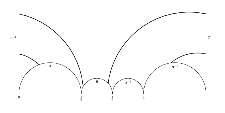
Figure 1 The closed geodesic on $Y_0(11)$
associated to the principal class in
$Y_0(11)$
associated to the principal class in $\mathbb {Q}(\sqrt {23})$
.
$\mathbb {Q}(\sqrt {23})$
.
1.3 Geometric interpretation
We will now explain the geometric content of Theorem 1.1. Recall that topologically, $Y_0(p)$
is a genus g curve with two punctures where the genus satisfies
$Y_0(p)$
is a genus g curve with two punctures where the genus satisfies $g=\frac {p}{12}+O(1)$
. We are interested in understanding the sum of the homology classes of the oriented closed geodesics of the principal genus. The associated geodesics will travel around
$g=\frac {p}{12}+O(1)$
. We are interested in understanding the sum of the homology classes of the oriented closed geodesics of the principal genus. The associated geodesics will travel around $Y_0(p)$
in a complicated way but our results can be interpreted as saying that
$Y_0(p)$
in a complicated way but our results can be interpreted as saying that
 $$ \begin{align*}\textit{`closed geodesics from the principal genus wind around the cusp at infinity a lot'}.\end{align*} $$
To illustrate this, let us consider the simplest nontrivial case $p=11$
where the genus is one. A fundamental polygon for
$p=11$
where the genus is one. A fundamental polygon for $Y_0(11)$
is given by the hyperbolic polygon with vertices
$Y_0(11)$
is given by the hyperbolic polygon with vertices $\infty , 0, \tfrac {1}{3},\tfrac {1}{2},\tfrac {2}{3},1$
as illustrated in Figure 1. The associated side pairing transformations (forgetting inverses) are
$\infty , 0, \tfrac {1}{3},\tfrac {1}{2},\tfrac {2}{3},1$
as illustrated in Figure 1. The associated side pairing transformations (forgetting inverses) are
which define a set of free generators for $\Gamma _0(11)$
(this follows from Poincaré’s Theorem as explained in Section 4). As illustrated in Figure 2, when viewing
$\Gamma _0(11)$
(this follows from Poincaré’s Theorem as explained in Section 4). As illustrated in Figure 2, when viewing $Y_0(11)$
as a double punctured torus, the matrix T corresponds to a simple loop around the puncture at
$Y_0(11)$
as a double punctured torus, the matrix T corresponds to a simple loop around the puncture at $\infty $
, and
$\infty $
, and $A,B$
correspond to the loops going around the two ‘holes’ of the torus. The content of Theorem 1.1 is concerned with the coordinates of the closed geodesics in the basis
$A,B$
correspond to the loops going around the two ‘holes’ of the torus. The content of Theorem 1.1 is concerned with the coordinates of the closed geodesics in the basis $\{T,A,B\}$
in the homology (or equivalently, when the corresponding hyperbolic conjugacy classes are projected to the abelinization of
$\{T,A,B\}$
in the homology (or equivalently, when the corresponding hyperbolic conjugacy classes are projected to the abelinization of $\Gamma _0(11)$
). Now consider the quadratic field
$\Gamma _0(11)$
). Now consider the quadratic field $K=\mathbb {Q}(\sqrt {23})$
which has narrow class number two and wide class number one. In this case, we have associated to the principal class
$K=\mathbb {Q}(\sqrt {23})$
which has narrow class number two and wide class number one. In this case, we have associated to the principal class $I\in \mathrm {Cl}_K^+$
the conjugacy class of the following matrix:
$I\in \mathrm {Cl}_K^+$
the conjugacy class of the following matrix:
and one can check that we have
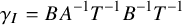 $$ \begin{align*}\gamma_I=BA^{-1}T^{-1} B^{-1}T^{-1}\end{align*} $$
in our basis (see Figure 1). Observe that $Y_0(11)$
is homotopic to a wedge of three circles, and we are counting the (oriented) number of times the geodesic goes around each of the three circles as illustrated in Figure 2. We already see in this numerically very small example a tendency towards large T-coordinate.
$Y_0(11)$
is homotopic to a wedge of three circles, and we are counting the (oriented) number of times the geodesic goes around each of the three circles as illustrated in Figure 2. We already see in this numerically very small example a tendency towards large T-coordinate.
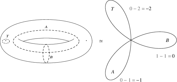
Figure 2 The $\{T,A,B\}$
-coordinates in the homology of
$\{T,A,B\}$
-coordinates in the homology of $Y_0(11)$
of the closed geodesic associated to the principal class of
$Y_0(11)$
of the closed geodesic associated to the principal class of $\mathbb {Q}(\sqrt {23})$
.
$\mathbb {Q}(\sqrt {23})$
. $\qquad $
Remark 1.9. Our results can be interpreted in the context of the classical problem of understanding the distribution of the projection
 $$ \begin{align} \pi_1(M)\twoheadrightarrow \mathrm{Conj}(\pi_1(M))\twoheadrightarrow \pi_1(M)^{\mathrm{ab}}\cong H_1(M,\mathbb{Z})\end{align} $$
for a manifold M. Note that if $\Gamma _0(p)$
is torsion free, then we have
$\Gamma _0(p)$
is torsion free, then we have $\pi _1(Y_0(p))\cong \Gamma _0(p)$
and
$\pi _1(Y_0(p))\cong \Gamma _0(p)$
and $H_1(Y_0(p), \mathbb {Z})\cong \Gamma _0(p)^{\mathrm {ab}}$
. For M a compact Riemann surface, there is a
$H_1(Y_0(p), \mathbb {Z})\cong \Gamma _0(p)^{\mathrm {ab}}$
. For M a compact Riemann surface, there is a $1$
-to-
$1$
-to- $1$
correspondence between conjugacy classes in
$1$
correspondence between conjugacy classes in $\pi _1(M)$
and oriented closed geodesics. Phillips and Sarnak [Reference Phillips and SarnakPS87] obtained an asymptotic expansion for the number of primitive geodesics of length
$\pi _1(M)$
and oriented closed geodesics. Phillips and Sarnak [Reference Phillips and SarnakPS87] obtained an asymptotic expansion for the number of primitive geodesics of length $\leq X$
with specified image under the map (1.12). In the same setup, Petridis and Risager [Reference Petridis and RisagerPR08] obtained an equidistribution statement for subsets
$\leq X$
with specified image under the map (1.12). In the same setup, Petridis and Risager [Reference Petridis and RisagerPR08] obtained an equidistribution statement for subsets $A\subset H_1(M,\mathbb {Z})$
with asymptotic density. Also, Petridis and Risager [Reference Petridis and RisagerPR05] showed that given a splitting
$A\subset H_1(M,\mathbb {Z})$
with asymptotic density. Also, Petridis and Risager [Reference Petridis and RisagerPR05] showed that given a splitting $H_1(M,\mathbb {Z})=\mathbb {Z} v \oplus V $
with
$H_1(M,\mathbb {Z})=\mathbb {Z} v \oplus V $
with $v\in H_1(M,\mathbb {Z})$
, the v-coordinate of closed geodesics become normally distributed (when properly normalized) again ordered by the length of the geodesics. See also [Reference Nordentoft and ConstantinescuNC20], [Reference Burrin and von EssenBv22]. From an arithmetic point of view, the ordering by geodesic length is not very natural as it gives very large weight to discriminants with a large class group (compared to the discriminant), whereas the ordering by discriminant does not seem to admit any nice geometric description.
$v\in H_1(M,\mathbb {Z})$
, the v-coordinate of closed geodesics become normally distributed (when properly normalized) again ordered by the length of the geodesics. See also [Reference Nordentoft and ConstantinescuNC20], [Reference Burrin and von EssenBv22]. From an arithmetic point of view, the ordering by geodesic length is not very natural as it gives very large weight to discriminants with a large class group (compared to the discriminant), whereas the ordering by discriminant does not seem to admit any nice geometric description.
2 Supersingular reduction of CM elliptic curves
The result of Duke [Reference DukeDuk88] mentioned in the introduction regarding equidistribution of closed geodesics has an imaginary quadratic analogue, which amounts to the equidistribution of elliptic curves with complex multiplication inside the moduli space of elliptic curves over $\mathbb {C}$
(i.e., CM points on the modular curve; see again [Reference DukeDuk88]). Similarly, our results can be seen as a real quadratic analogue of the distribution of the supersingular reduction of elliptic curves with complex multiplication as investigated by many authors [Reference MichelMic04], [Reference Elkies, Ono and YangEOY05], [Reference YangYan08], [Reference KaneKan09], [Reference Liu, Masri and YoungLMY15], [Reference Aka, Luethi, Michel and WieserALMW22]. This analogy between oriented closed geodesics in homology and supersingular reduction of CM elliptic curves is very natural and appears, for example, in the recent work of Darmon–Harris–Rotger–Venkatesh [Reference Darmon, Harris, Rotger and VenkateshDHRV21].
$\mathbb {C}$
(i.e., CM points on the modular curve; see again [Reference DukeDuk88]). Similarly, our results can be seen as a real quadratic analogue of the distribution of the supersingular reduction of elliptic curves with complex multiplication as investigated by many authors [Reference MichelMic04], [Reference Elkies, Ono and YangEOY05], [Reference YangYan08], [Reference KaneKan09], [Reference Liu, Masri and YoungLMY15], [Reference Aka, Luethi, Michel and WieserALMW22]. This analogy between oriented closed geodesics in homology and supersingular reduction of CM elliptic curves is very natural and appears, for example, in the recent work of Darmon–Harris–Rotger–Venkatesh [Reference Darmon, Harris, Rotger and VenkateshDHRV21].
Let $\mathcal {E\ell \ell }^{ss}(\mathbb {F}_{p^2})=\{e_1,\ldots , e_n\}$
denote the set of isomorphism classes of supersingular elliptic curves defined over
$\mathcal {E\ell \ell }^{ss}(\mathbb {F}_{p^2})=\{e_1,\ldots , e_n\}$
denote the set of isomorphism classes of supersingular elliptic curves defined over $\mathbb {F}_{p^2}$
. It is known that
$\mathbb {F}_{p^2}$
. It is known that $|\mathcal {E\ell \ell }^{ss}(\mathbb {F}_{p^2})|=\frac {p}{12}+O(1)$
. We endow
$|\mathcal {E\ell \ell }^{ss}(\mathbb {F}_{p^2})|=\frac {p}{12}+O(1)$
. We endow $\mathcal {E\ell \ell }^{ss}(\mathbb {F}_{p^2})$
with the measure defined by
$\mathcal {E\ell \ell }^{ss}(\mathbb {F}_{p^2})$
with the measure defined by
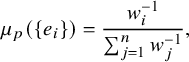 $$ \begin{align}\mu_p(\{e_i\})= \frac{w_i^{-1}}{\sum_{j=1}^n w_j^{-1}},\end{align} $$
where $w_i$
denotes the size of the endomorphism group of the elliptic curves corresponding to
$w_i$
denotes the size of the endomorphism group of the elliptic curves corresponding to $e_i$
. Let
$e_i$
. Let $\mathcal {E\ell \ell }_K$
denote the set of isomorphism classes of elliptic curve (defined over
$\mathcal {E\ell \ell }_K$
denote the set of isomorphism classes of elliptic curve (defined over $\overline {\mathbb {Q}}$
) with complex multiplication by the ring of integers of the imaginary quadratic field K with discriminant
$\overline {\mathbb {Q}}$
) with complex multiplication by the ring of integers of the imaginary quadratic field K with discriminant $d_K <0$
and class group
$d_K <0$
and class group $\mathrm {Cl}_K$
. The set
$\mathrm {Cl}_K$
. The set $\mathcal {E\ell \ell }_K$
carries a natural
$\mathcal {E\ell \ell }_K$
carries a natural $\mathrm {Cl}_K$
-action which is free and transitive. If p is inert in K, we have a map
$\mathrm {Cl}_K$
-action which is free and transitive. If p is inert in K, we have a map
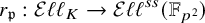 $$ \begin{align*}r_{\mathfrak{p}}:\mathcal{E\ell\ell}_K\rightarrow \mathcal{E\ell\ell}^{ss}(\mathbb{F}_{p^2})\end{align*} $$
given by taking the mod $\mathfrak {p}$
reduction where
$\mathfrak {p}$
reduction where $\mathfrak {p}$
is a prime ideal of the Hilbert class field of K lying over p. The following is [Reference MichelMic04, Theorem 3].
$\mathfrak {p}$
is a prime ideal of the Hilbert class field of K lying over p. The following is [Reference MichelMic04, Theorem 3].
Theorem 2.1 (Michel)
Consider a CM elliptic curve $E\in \mathcal {E\ell \ell }_K$
and a subgroup
$E\in \mathcal {E\ell \ell }_K$
and a subgroup $H\leq \mathrm {Cl}_K$
of index
$H\leq \mathrm {Cl}_K$
of index $\leq |d_K|^{1/2015}$
. Then the orbits
$\leq |d_K|^{1/2015}$
. Then the orbits $H.E=\{r_{\mathfrak {p}}(A.E)\in \mathcal {E\ell \ell }^{ss}(\mathbb {F}_{p^2}):A \in H \}$
become equidistributed as
$H.E=\{r_{\mathfrak {p}}(A.E)\in \mathcal {E\ell \ell }^{ss}(\mathbb {F}_{p^2}):A \in H \}$
become equidistributed as $d_K \rightarrow -\infty $
with respect to the measure
$d_K \rightarrow -\infty $
with respect to the measure $\mu _p$
given by (2.1).
$\mu _p$
given by (2.1).
The proof goes through an identification of $\mathcal {E\ell \ell }^{ss}(\mathbb {F}_{p^2})$
with the set of connected components of a certain conic curve
$\mathcal {E\ell \ell }^{ss}(\mathbb {F}_{p^2})$
with the set of connected components of a certain conic curve
 $$ \begin{align} X^{p,\infty}:=\mathbf{PB}^\times(\mathbb{Q}) \backslash \mathbf{PB}^\times(\mathbb{A}_{\mathbb{Q}}) /\mathbf{PB}^\times(\widehat{\mathbb{Z}}) K_\infty,\end{align} $$
where $\mathbf {B}$
denotes the unique quaternion algebra over
$\mathbf {B}$
denotes the unique quaternion algebra over $\mathbb {Q}$
ramified at p and
$\mathbb {Q}$
ramified at p and $\infty $
,
$\infty $
, $\mathbf {PB}^\times $
is its group of projective units,
$\mathbf {PB}^\times $
is its group of projective units, $K_\infty $
denotes a maximal compact torus of
$K_\infty $
denotes a maximal compact torus of $\mathbf {PB}^\times (\mathbb {R})$
and
$\mathbf {PB}^\times (\mathbb {R})$
and $\mathbf {PB}^\times (\widehat {\mathbb {Z}})$
denotes the projective units of
$\mathbf {PB}^\times (\widehat {\mathbb {Z}})$
denotes the projective units of $\widehat {\mathbb {Z}}\otimes \mathcal {O}$
where
$\widehat {\mathbb {Z}}\otimes \mathcal {O}$
where $\mathcal {O}\subset \mathbf {B}$
is a maximal order. Using the Jacquet–Langlands correspondence and a formula of Gross, this reduces the distribution problem to subconvexity bounds of certain Rankin–Selberg L-functions which is resolved (see [Reference MichelMic04, Section 5] for details).
$\mathcal {O}\subset \mathbf {B}$
is a maximal order. Using the Jacquet–Langlands correspondence and a formula of Gross, this reduces the distribution problem to subconvexity bounds of certain Rankin–Selberg L-functions which is resolved (see [Reference MichelMic04, Section 5] for details).
In order to set up the analogy with the real quadratic case, we will slightly reformulate the statement in Theorem 2.1 above. Denote by $H_0(X^{p,\infty },\mathbb {Z})$
the
$H_0(X^{p,\infty },\mathbb {Z})$
the $0$
-th (singular) homology group of
$0$
-th (singular) homology group of $X^{p,\infty }$
with integral coefficients (one should picture a copy of
$X^{p,\infty }$
with integral coefficients (one should picture a copy of $\mathbb {Z}$
at each connected component of
$\mathbb {Z}$
at each connected component of $X^{p,\infty }$
), which is a lattice inside the real homology group
$X^{p,\infty }$
), which is a lattice inside the real homology group $H_0(X^{p,\infty },\mathbb {R})$
. Note that both of these abelian groups carry a natural action of the Hecke algebra coming from the description in terms of quaternion algebras (see, for example, [Reference Bertolini and DarmonBD96, Section 1.5]), and as such is isomorphic to the space of modular forms
$H_0(X^{p,\infty },\mathbb {R})$
. Note that both of these abelian groups carry a natural action of the Hecke algebra coming from the description in terms of quaternion algebras (see, for example, [Reference Bertolini and DarmonBD96, Section 1.5]), and as such is isomorphic to the space of modular forms $\mathcal {M}_2(p)$
of level p and weight
$\mathcal {M}_2(p)$
of level p and weight $2$
. We have a natural basis of
$2$
. We have a natural basis of $H_0(X^{p,\infty },\mathbb {Z})$
of geometric nature corresponding to the classes
$H_0(X^{p,\infty },\mathbb {Z})$
of geometric nature corresponding to the classes $e_1,\ldots , e_n$
(using suggestive notation) associated to each connected component of
$e_1,\ldots , e_n$
(using suggestive notation) associated to each connected component of $X^{p,\infty }$
. In this basis, the Eisenstein element is the following:
$X^{p,\infty }$
. In this basis, the Eisenstein element is the following:
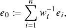 $$ \begin{align*} e_0:= \sum_{i=1}^n w_i^{-1}e_i, \end{align*} $$
meaning that $T_\ell e_0=(\ell +1)e_0$
for
$T_\ell e_0=(\ell +1)e_0$
for $\ell \neq p$
prime and
$\ell \neq p$
prime and $T_\ell $
the
$T_\ell $
the $\ell $
-th Hecke operator. Using the above identifications with supersingular elliptic curves and after fixing an elliptic curve
$\ell $
-th Hecke operator. Using the above identifications with supersingular elliptic curves and after fixing an elliptic curve $E\in \mathcal {E\ell \ell }_K$
, we get a map
$E\in \mathcal {E\ell \ell }_K$
, we get a map
 $$ \begin{align}r_p: \mathrm{Cl}_K\rightarrow \{e_1,\ldots, e_n\}\subset H_0(X^{p,\infty},\mathbb{Z})\subset H_0(X^{p,\infty},\mathbb{R}),\quad A\mapsto r_{\mathfrak{p}}(A.E),\end{align} $$
which will serve as an imaginary quadratic analogue of the map (1.2). We will now consider Theorem 2.1 as a statement about convergence (with respect to the standard topology) on the $(n-1)$
-sphere which we identity with
$(n-1)$
-sphere which we identity with $\mathbf {S}(V_{p,\infty }):=(V_{p,\infty }-\{0\})/\mathbb {R}_{>0}$
equipped with the quotient toplogy where
$\mathbf {S}(V_{p,\infty }):=(V_{p,\infty }-\{0\})/\mathbb {R}_{>0}$
equipped with the quotient toplogy where $V_{p,\infty }:=H_0(X^{p,\infty },\mathbb {R})\cong \mathbb {R}^{n}$
(equipped with the Euclidean topology). As above for
$V_{p,\infty }:=H_0(X^{p,\infty },\mathbb {R})\cong \mathbb {R}^{n}$
(equipped with the Euclidean topology). As above for $v\in V_{p,\infty }-\{0\}$
, we denote by
$v\in V_{p,\infty }-\{0\}$
, we denote by $\overline {v}\in \mathbf {S}(V_{p,\infty })$
the image under the natural projection
$\overline {v}\in \mathbf {S}(V_{p,\infty })$
the image under the natural projection $V_{p,\infty }-\{0\}\twoheadrightarrow \mathbf {S}(V_{p,\infty })$
. We can then recast the equidistribution statement of Michel as follows.
$V_{p,\infty }-\{0\}\twoheadrightarrow \mathbf {S}(V_{p,\infty })$
. We can then recast the equidistribution statement of Michel as follows.
Theorem 2.2 (‘Vector space’-version of Theorem 2.1)
Let $p>2$
be prime and let K be an imaginary quadratic field of discriminant
$p>2$
be prime and let K be an imaginary quadratic field of discriminant $d_K <0$
such that p is inert in K. Consider a subgroup
$d_K <0$
such that p is inert in K. Consider a subgroup $H\leq \mathrm {Cl}_K$
of index
$H\leq \mathrm {Cl}_K$
of index $\leq |d_K|^{1/2015}$
and a coset
$\leq |d_K|^{1/2015}$
and a coset $CH\subset \mathrm {Cl}_K$
. Then we have as
$CH\subset \mathrm {Cl}_K$
. Then we have as $d_K \rightarrow -\infty $
that
$d_K \rightarrow -\infty $
that
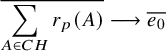 $$ \begin{align}\overline{\sum_{A \in CH} r_p(A)} \longrightarrow \overline{e_0} \end{align} $$
in the standard topology of $\mathbf {S}(V_{p,\infty })$
.
$\mathbf {S}(V_{p,\infty })$
.
We will now show that this is equivalent to Theorem 2.1. Let $B=\{e_1,\ldots , e_n\}$
be the standard basis for
$B=\{e_1,\ldots , e_n\}$
be the standard basis for $V_{p,\infty }$
which defines an isomorphism
$V_{p,\infty }$
which defines an isomorphism $V_{p,\infty }\cong \mathbb {R}^n$
. As explained above, we get a norm
$V_{p,\infty }\cong \mathbb {R}^n$
. As explained above, we get a norm $|\!|\cdot |\!|_{B,1}$
on
$|\!|\cdot |\!|_{B,1}$
on $V_{p,\infty }$
by pulling back the
$V_{p,\infty }$
by pulling back the $L^1$
-norm in the standard basis of
$L^1$
-norm in the standard basis of $\mathbb {R}^n$
. Now recall that the convergence on the
$\mathbb {R}^n$
. Now recall that the convergence on the $(n-1)$
-sphere
$(n-1)$
-sphere $\mathbf {S}(V_{p,\infty })$
is equivalent to the convergence statement (1.8) using, for example, the norm
$\mathbf {S}(V_{p,\infty })$
is equivalent to the convergence statement (1.8) using, for example, the norm $|\!|\cdot |\!|_{B,1}$
. Notice that we have
$|\!|\cdot |\!|_{B,1}$
. Notice that we have
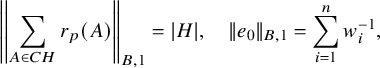 $$ \begin{align*} \left|\left|\sum_{A \in CH} r_p(A) \right|\right|_{B,1}=|H|,\quad |\!|e_0 |\!|_{B,1}=\sum_{i=1}^n w_i^{-1},\end{align*} $$
recalling that the $e_i$
-coordinate of
$e_i$
-coordinate of $e_0$
is equal to
$e_0$
is equal to $w_i^{-1}$
. Now the convergence in (1.8) implies that the
$w_i^{-1}$
. Now the convergence in (1.8) implies that the $e_i$
-coordinates of
$e_i$
-coordinates of $\sum _{A \in CH} r_p(A)$
converge to those of
$\sum _{A \in CH} r_p(A)$
converge to those of $e_0$
(both normalized). This recovers the statement of Michel as in Theorem 2.1 up to the fact that Theorem 2.2 does not see that
$e_0$
(both normalized). This recovers the statement of Michel as in Theorem 2.1 up to the fact that Theorem 2.2 does not see that $r_p(A)$
is always equal to one of the vectors
$r_p(A)$
is always equal to one of the vectors $e_1,\ldots , e_n$
.
$e_1,\ldots , e_n$
.
2.1 Supersingular reduction of elliptic curves of varying level
It is natural to ask what happens if we let p vary with $d_K $
as has been considered by Liu–Masri–Young [Reference Liu, Masri and YoungLMY15]. In the above terminology, they consider the convergence with respect to the basis corresponding to the connected components
$d_K $
as has been considered by Liu–Masri–Young [Reference Liu, Masri and YoungLMY15]. In the above terminology, they consider the convergence with respect to the basis corresponding to the connected components $\{e_1,\ldots , e_n\}$
of
$\{e_1,\ldots , e_n\}$
of $X^{p,\infty }$
. Then [Reference Liu, Masri and YoungLMY15, Theorem 1.1] amounts to the following:
$X^{p,\infty }$
. Then [Reference Liu, Masri and YoungLMY15, Theorem 1.1] amounts to the following:
 $$ \begin{align} \left| \left|\frac{\sum_{A \in \mathrm{Cl}_K} r_p(A)}{|\!|\sum_{A \in \mathrm{Cl}_K} r_p(A)|\!|_{B,1}}-\frac{e_0}{|\!|e_0|\!|_{B,1}}\right|\right|_{B,\infty} \ll_\varepsilon p^{1/8+\varepsilon} |d_K|^{-1/16+\varepsilon}, \end{align} $$
where again, $|\!| \cdot |\!|_{B,1}$
and
$|\!| \cdot |\!|_{B,1}$
and $|\!| \cdot |\!|_{B,\infty }$
denote the pullback of, respectively, the
$|\!| \cdot |\!|_{B,\infty }$
denote the pullback of, respectively, the $L^1$
-norm and sup norm under the isomorphism
$L^1$
-norm and sup norm under the isomorphism $V_{p,\infty }\cong \mathbb {R}^n$
defined by
$V_{p,\infty }\cong \mathbb {R}^n$
defined by $B=\{e_1,\ldots , e_n\}$
. We note that the statement (2.5) is exactly parallel to Theorem 1.5. Translating back to the language of elliptic curves, (2.5) implies the following analogue of Linnik’s Theorem on the smallest prime in arithmetic progressions.
$B=\{e_1,\ldots , e_n\}$
. We note that the statement (2.5) is exactly parallel to Theorem 1.5. Translating back to the language of elliptic curves, (2.5) implies the following analogue of Linnik’s Theorem on the smallest prime in arithmetic progressions.
Theorem 2.3 (Liu–Masri–Young)
The reduction map $r_{\mathfrak {q}} : \mathcal {E\ell \ell }_K \rightarrow \mathcal {E\ell \ell }^{ss}_{p^2}$
is surjective for
$r_{\mathfrak {q}} : \mathcal {E\ell \ell }_K \rightarrow \mathcal {E\ell \ell }^{ss}_{p^2}$
is surjective for ${|d_K| \gg _\varepsilon p^{18+\varepsilon }}$
.
${|d_K| \gg _\varepsilon p^{18+\varepsilon }}$
.
We think of Corollary 1.7 (and more generally Corollary 8.1 below) as a real quadratic analogue of the above.
3 Arithmetic background
In this section, we will introduce some basic facts about, respectively, oriented closed geodesics associated to class groups of real quadratic fields and (co)homology of modular curves.
3.1 Real quadratic fields and closed geodesics
We will refer to [Reference PopaPop06] and [Reference DarmonDar94] for an in-depth account of the following material. Let K be a real quadratic extension of $\mathbb {Q}$
of discriminant
$\mathbb {Q}$
of discriminant $d_K>0$
. Let p be a prime which splits in K and fix throughout a residue
$d_K>0$
. Let p be a prime which splits in K and fix throughout a residue $r \ \mathrm {mod}\ 2p$
such that
$r \ \mathrm {mod}\ 2p$
such that $r^2\equiv d_K \ \mathrm {mod}\ 4p$
. Then we have the following equality of ideals:
$r^2\equiv d_K \ \mathrm {mod}\ 4p$
. Then we have the following equality of ideals:
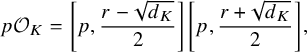 $$ \begin{align*} p\mathcal{O}_K= \left[p,\frac{r-\sqrt{d_K}}{2}\right]\left[p,\frac{r+\sqrt{d_K}}{2}\right],\end{align*} $$
where we use the following notation for $\alpha ,\beta \in K$
:
$\alpha ,\beta \in K$
:
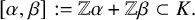 $$ \begin{align}[\alpha,\beta]:=\mathbb{Z}\alpha+\mathbb{Z}\beta \subset K.\end{align} $$
In other words, $[p,\frac {r\pm \sqrt {d_K}}{2}]$
are the two prime ideals of
$[p,\frac {r\pm \sqrt {d_K}}{2}]$
are the two prime ideals of $\mathcal {O}_K$
lying over p.
$\mathcal {O}_K$
lying over p.
We let $\mathrm {Cl}_K^+$
denote the narrow class group of K (i.e., fractional ideals modulo principal ideals generated by elements of positive norms). Below, when the discriminant
$\mathrm {Cl}_K^+$
denote the narrow class group of K (i.e., fractional ideals modulo principal ideals generated by elements of positive norms). Below, when the discriminant $d_K $
is clear from context, we let
$d_K $
is clear from context, we let $I\in \mathrm {Cl}_K^+$
denote the class containing the principal fractional ideal
$I\in \mathrm {Cl}_K^+$
denote the class containing the principal fractional ideal $(1)=\mathcal {O}_K\subset K $
and
$(1)=\mathcal {O}_K\subset K $
and $J\in \mathrm {Cl}_K^+$
denote the class containing the different
$J\in \mathrm {Cl}_K^+$
denote the class containing the different $(\sqrt {d_K})=\sqrt {d_K}\mathcal {O}_K\subset K $
. Observe that for fundamental discriminants divisible by a prime
$(\sqrt {d_K})=\sqrt {d_K}\mathcal {O}_K\subset K $
. Observe that for fundamental discriminants divisible by a prime $q\equiv 3 \ \mathrm {mod}\ 4$
, there exists no unit with norm
$q\equiv 3 \ \mathrm {mod}\ 4$
, there exists no unit with norm $-1$
(as
$-1$
(as $-1$
is not a quadratic residue modulo q) which implies that
$-1$
is not a quadratic residue modulo q) which implies that $J\neq I$
. In this case, a principal ideal belongs to the class J exactly if it has a generator with negative norm.
$J\neq I$
. In this case, a principal ideal belongs to the class J exactly if it has a generator with negative norm.
We will now show the following result, which is closely related to the conditions appearing in our main results as we will see below.
Proposition 3.1. Let p be an odd prime. Then there exists infinitely many positive fundamental discriminants d such that $J\neq I$
and
$J\neq I$
and $[p,\frac {r-\sqrt {d}}{2}]\in J$
inside
$[p,\frac {r-\sqrt {d}}{2}]\in J$
inside $\mathrm {Cl}_K^+ $
with
$\mathrm {Cl}_K^+ $
with $K=\mathbb {Q}(\sqrt {d})$
.
$K=\mathbb {Q}(\sqrt {d})$
.
Proof. Pick an odd prime $q\equiv 3 \ \mathrm {mod}\ 4$
such that
$q\equiv 3 \ \mathrm {mod}\ 4$
such that $-p$
is a quadratic residue mod q. Then by simple considerations about quadratic residues, there is a residue
$-p$
is a quadratic residue mod q. Then by simple considerations about quadratic residues, there is a residue $t \ \mathrm {mod}\ 8 q$
such that
$t \ \mathrm {mod}\ 8 q$
such that
 $$ \begin{align*} q| t^2+p,\, \, q^2\!\!\not| t^2+p \quad \text{and}\quad (t^2+p \ \mathrm {mod}\ 16)\in \{ 1, 5, 8,9,12,13\}, \end{align*} $$
meaning in particular that $t^2+p\equiv 0\text { or }1 \ \mathrm {mod}\ 4$
. Now for each
$t^2+p\equiv 0\text { or }1 \ \mathrm {mod}\ 4$
. Now for each $n\equiv t \ \mathrm {mod}\ 8q$
, there is a unique positive fundamental discriminant
$n\equiv t \ \mathrm {mod}\ 8q$
, there is a unique positive fundamental discriminant $d>0$
and integer
$d>0$
and integer $m>0$
such that
$m>0$
such that $d m^2=n^2+p$
. By construction, we have
$d m^2=n^2+p$
. By construction, we have $q| d$
, and thus
$q| d$
, and thus $J\neq I$
inside
$J\neq I$
inside $\mathrm {Cl}_K^+$
where
$\mathrm {Cl}_K^+$
where $K=\mathbb {Q}(\sqrt {d})$
. Furthermore, we have the factorization
$K=\mathbb {Q}(\sqrt {d})$
. Furthermore, we have the factorization
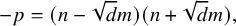 $$ \begin{align*} -p=(n-\sqrt{d}m)(n+\sqrt{d}m), \end{align*} $$
which means that $[p,\frac {r-\sqrt {d}}{2}]$
is a principal ideal generated by
$[p,\frac {r-\sqrt {d}}{2}]$
is a principal ideal generated by $ n\pm \sqrt {d}m$
(for some choice of sign
$ n\pm \sqrt {d}m$
(for some choice of sign $\pm $
). By construction, the norm of
$\pm $
). By construction, the norm of $n\pm \sqrt {d}m$
is negative (and equal to
$n\pm \sqrt {d}m$
is negative (and equal to $-p$
). By the above, this implies
$-p$
). By the above, this implies $[p,\frac {r-\sqrt {d}}{2}]\in J$
in
$[p,\frac {r-\sqrt {d}}{2}]\in J$
in $\mathrm {Cl}_K^+$
as wanted.
$\mathrm {Cl}_K^+$
as wanted.
Now it follows that if $J\neq I$
, then
$J\neq I$
, then $J\notin (\mathrm {Cl}_K^+)^2$
. Thus, for
$J\notin (\mathrm {Cl}_K^+)^2$
. Thus, for $p,d$
as in Proposition 3.1 and each subgroup
$p,d$
as in Proposition 3.1 and each subgroup $H\leq (\mathrm {Cl}_K^+)^2$
, we have
$H\leq (\mathrm {Cl}_K^+)^2$
, we have $[p,\frac {r-\sqrt {d}}{2}]\notin H$
. This gives plenty of examples for which Theorems 1.1 and 1.5 apply, recalling that
$[p,\frac {r-\sqrt {d}}{2}]\notin H$
. This gives plenty of examples for which Theorems 1.1 and 1.5 apply, recalling that $\{\mathfrak {p}_1, \mathfrak {p}_2\}=\{[p,\frac {r\pm \sqrt {d}}{2}]\} $
.
$\{\mathfrak {p}_1, \mathfrak {p}_2\}=\{[p,\frac {r\pm \sqrt {d}}{2}]\} $
.
3.1.1 Closed geodesics and class groups
Let p be prime and K a real quadratic field of discriminant $d_K$
such that p splits in K. Let
$d_K$
such that p splits in K. Let $r \ \mathrm {mod}\ 2p$
as above be such that
$r \ \mathrm {mod}\ 2p$
as above be such that $r^2\equiv d_K \ \mathrm {mod}\ 4p$
. Denote by
$r^2\equiv d_K \ \mathrm {mod}\ 4p$
. Denote by $\mathcal {Q}_{K,p}$
(suppressing r in the notation) the set of all integral binary quadratic form
$\mathcal {Q}_{K,p}$
(suppressing r in the notation) the set of all integral binary quadratic form
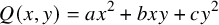 $$ \begin{align*}Q(x,y)=ax^2+bxy+cy^2\end{align*} $$
of discriminant $b^2-4ac=d_K$
and level p, meaning that
$b^2-4ac=d_K$
and level p, meaning that $a\equiv 0 \ \mathrm {mod}\ p$
and
$a\equiv 0 \ \mathrm {mod}\ p$
and $b\equiv r \ \mathrm {mod}\ 2p$
. The group
$b\equiv r \ \mathrm {mod}\ 2p$
. The group $\Gamma _0(p)$
acts naturally on
$\Gamma _0(p)$
acts naturally on $\mathcal {Q}_{K,p}$
by coordinate transformation. It is a classical fact, essentially due to Gauß, that there is a natural bijection (depending on the choice of
$\mathcal {Q}_{K,p}$
by coordinate transformation. It is a classical fact, essentially due to Gauß, that there is a natural bijection (depending on the choice of $r \ \mathrm {mod}\ p$
)
$r \ \mathrm {mod}\ p$
)
 $$ \begin{align} \mathrm{Cl}_K^+ \xrightarrow{\sim} \Gamma_0(p)\backslash \mathcal{Q}_{K,p}. \end{align} $$
When the level is trivial, the above bijection is induced by mapping $ax^2+bxy+cy^2$
to the narrow ideal class of the fractional ideal
$ax^2+bxy+cy^2$
to the narrow ideal class of the fractional ideal $[1,\frac {-\mathrm {sign}(a)b+\sqrt {d_K}}{2|a|}]$
(using the notation (3.1)).
$[1,\frac {-\mathrm {sign}(a)b+\sqrt {d_K}}{2|a|}]$
(using the notation (3.1)).
Given an integral binary quadratic form $Q(x,y)=ax^2+bxy+cy^2$
of discriminant
$Q(x,y)=ax^2+bxy+cy^2$
of discriminant $d_K $
and level p, we associate the following matrix:
$d_K $
and level p, we associate the following matrix:
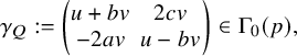 $$ \begin{align}\gamma_Q:=\begin{pmatrix} u+bv & 2cv \\ -2av & u-bv\end{pmatrix}\in \Gamma_0(p),\end{align} $$
where $u,v$
are positive half-integers satisfying Pell’s equation
$u,v$
are positive half-integers satisfying Pell’s equation $u^2-d_Kv^2=1$
and such that v is minimal among all such solutions (i.e., the fundamental positive unit of K is
$u^2-d_Kv^2=1$
and such that v is minimal among all such solutions (i.e., the fundamental positive unit of K is $\epsilon _K=u+v\sqrt {d_K}$
).
$\epsilon _K=u+v\sqrt {d_K}$
).
For $A\in \mathrm {Cl}_K^+$
, we denote by
$A\in \mathrm {Cl}_K^+$
, we denote by $\mathcal {C}_{A}(p)$
the oriented closed geodesic on
$\mathcal {C}_{A}(p)$
the oriented closed geodesic on $Y_0(p)$
obtained by projecting the oriented geodesic connecting
$Y_0(p)$
obtained by projecting the oriented geodesic connecting $z_Q$
and
$z_Q$
and $\gamma _Q z_Q$
, where
$\gamma _Q z_Q$
, where
 $$ \begin{align*} z_Q:=\frac{-\mathrm{sign} (a)b+i \sqrt{d_K}}{2|a|} \end{align*} $$
and $Q\in \mathcal {Q}_{K,p}$
corresponds to A under the isomorphism (3.2) (the image in
$Q\in \mathcal {Q}_{K,p}$
corresponds to A under the isomorphism (3.2) (the image in $Y_0(p)$
is independent of the choice of representative Q).
$Y_0(p)$
is independent of the choice of representative Q).
3.2 (Co)homology of modular curves
Here and throughout, we will consider matrices in $\mathrm {SL}_2(\mathbb {R})$
as elements of
$\mathrm {SL}_2(\mathbb {R})$
as elements of $\mathrm {PSL}_2(\mathbb {R})$
without further mentioning. Let p be prime and consider the Hecke congruence group (or more precisely, its projection to
$\mathrm {PSL}_2(\mathbb {R})$
without further mentioning. Let p be prime and consider the Hecke congruence group (or more precisely, its projection to $\mathrm {PSL}_2(\mathbb {R})$
)
$\mathrm {PSL}_2(\mathbb {R})$
)
Let
 $$ \begin{align*}Y_0(p):=\Gamma_0(p)\backslash \mathbb{H},\quad X_0(p):=\overline{Y_0(p)}=Y_0(p)\cup \Gamma_0(p)\backslash \mathbb{P}^1(\mathbb{Q}) \end{align*} $$
be resp., the modular curve of level p and its compactification which is a compact Riemann surface of genus $g=\frac {p}{12}+O(1)$
(see, for example, [Reference ShimuraShi94, Proposition 1.40]). We can consider the integral singular homology group [Reference HatcherHat02, Chapter 2]
$g=\frac {p}{12}+O(1)$
(see, for example, [Reference ShimuraShi94, Proposition 1.40]). We can consider the integral singular homology group [Reference HatcherHat02, Chapter 2]
 $$ \begin{align*}H_1(Y_0(p),\mathbb{Z})\cong \mathbb{Z}^{2g+1}, \end{align*} $$
which sits as a lattice inside the real homology
 $$ \begin{align*}H_1(Y_0(p),\mathbb{R})\cong \mathbb{R}^{2g+1}. \end{align*} $$
We will be interested in the distribution of oriented closed geodesics inside the lattice $H_1(Y_0(p),\mathbb {Z})$
.
$H_1(Y_0(p),\mathbb {Z})$
.
We have the cap product pairing
 $$ \begin{align} \langle\cdot, \cdot \rangle: H_1(Y_0(p),\mathbb{R})\times H^1(Y_0(p),\mathbb{R})\rightarrow \mathbb{R}\end{align} $$
between real homology and cohomology which identifies $H^1(Y_0(p),\mathbb {R})$
with the linear dual
$H^1(Y_0(p),\mathbb {R})$
with the linear dual $H_1(Y_0(p),\mathbb {R})^\ast $
. Given a basis B of
$H_1(Y_0(p),\mathbb {R})^\ast $
. Given a basis B of $H_1(Y_0(p), \mathbb {R})$
, we denote by
$H_1(Y_0(p), \mathbb {R})$
, we denote by $ B^{\ast }\subset H^1(Y_0(p), \mathbb {R})$
the dual basis of B with respect to the cap product pairing as in (3.4).
$ B^{\ast }\subset H^1(Y_0(p), \mathbb {R})$
the dual basis of B with respect to the cap product pairing as in (3.4).
Recall that the de Rham isomorphism gives a description of $H^1(Y_0(p),\mathbb {R})$
in terms of real valued harmonic 1-forms on
$H^1(Y_0(p),\mathbb {R})$
in terms of real valued harmonic 1-forms on $Y_0(p)$
. Any such 1-form is a linear combination of forms of the type
$Y_0(p)$
. Any such 1-form is a linear combination of forms of the type
 $$ \begin{align*} \omega_f=2\pi i f(z)dz ,\quad \overline{\omega_f}=\overline{2\pi i f(z)dz}, \end{align*} $$
where $f\in \mathcal {M}_2(p)$
is a weight 2 and level p holomorphic form (not necessarily cuspidal). We also have a surjective map
$f\in \mathcal {M}_2(p)$
is a weight 2 and level p holomorphic form (not necessarily cuspidal). We also have a surjective map
 $$ \begin{align} \Gamma_0(p)\twoheadrightarrow H_1(Y_0(p), \mathbb{Z}),\quad \gamma\mapsto \{ z, \gamma z\},\end{align} $$
where $z\in \mathbb {H}$
(the class does not depend on the choice of z), and we are using the following notation for
$z\in \mathbb {H}$
(the class does not depend on the choice of z), and we are using the following notation for $z_1,z_2\in \mathbb {H}$
:
$z_1,z_2\in \mathbb {H}$
:
 $$ \begin{align}\{z_1, z_2\}:= [\text{class of the oriented geodesic connecting} z_1 \text{ and } z_2]\in H_1(Y_0(p), \mathbb{R}), \end{align} $$
which defines an element of the real homology $H_1(Y_0(p), \mathbb {R})$
via integration against
$H_1(Y_0(p), \mathbb {R})$
via integration against $1$
-forms. The map (3.5) induces an isomorphism
$1$
-forms. The map (3.5) induces an isomorphism
 $$ \begin{align}\Gamma_0(p)^{\mathrm{ab}}/(\Gamma_0(p)^{\mathrm{ab}})_{\mathrm{tor}}\cong H_1(Y_0(p),\mathbb{Z}).\end{align} $$
We note that for a closed oriented geodesic $\mathcal {C}_{A}(p)$
as in the previous section, the homology class
$\mathcal {C}_{A}(p)$
as in the previous section, the homology class $[\mathcal {C}_{A}(p)]\in H_1(Y_0(p),\mathbb {Z})$
corresponds exactly to the image of (any)
$[\mathcal {C}_{A}(p)]\in H_1(Y_0(p),\mathbb {Z})$
corresponds exactly to the image of (any) $\gamma _Q$
as in (3.3) under the map (3.5). Using the above identifications, the cap product pairing is induced by the map
$\gamma _Q$
as in (3.3) under the map (3.5). Using the above identifications, the cap product pairing is induced by the map
 $$ \begin{align*} \Gamma_0(p)\times \mathcal{M}_2(p)\ni (\gamma, f)\mapsto \int^{\gamma z}_z \omega_f, \end{align*} $$
for any $z\in \mathbb {H}$
.
$z\in \mathbb {H}$
.
The natural pullback map induced by inclusion fits into a short exact sequence of $\mathbb {R}$
-vector spaces
$\mathbb {R}$
-vector spaces
 $$ \begin{align} 0\rightarrow H^1(X_0(p),\mathbb{R})\rightarrow H^1(Y_0(p),\mathbb{R})\rightarrow \mathbb{R} \rightarrow 0, \end{align} $$
using here that we have two cusps (which, as we will see, implies that the Eisenstein space of weight $2$
is one-dimensional). This identifies
$2$
is one-dimensional). This identifies $H^1(X_0(p),\mathbb {R})$
with the parabolic classes in
$H^1(X_0(p),\mathbb {R})$
with the parabolic classes in $H^1(Y_0(p),\mathbb {R})$
(i.e., classes which vanish on all parabolic elements of
$H^1(Y_0(p),\mathbb {R})$
(i.e., classes which vanish on all parabolic elements of $\Gamma _0(p)$
using the above pairing). Under the de Rham isomorphism, the parabolic classes correspond to
$\Gamma _0(p)$
using the above pairing). Under the de Rham isomorphism, the parabolic classes correspond to $1$
-forms obtained from holomorphic cusp(!) forms of weight
$1$
-forms obtained from holomorphic cusp(!) forms of weight $2$
and level p (see, for example, [Reference ShimuraShi94, Section 5]). Similarly, we have the pushforward map
$2$
and level p (see, for example, [Reference ShimuraShi94, Section 5]). Similarly, we have the pushforward map $H_1(Y_0(p),\mathbb {R})\rightarrow H_1(X_0(p),\mathbb {R})$
whose kernel is exactly given by the image of the parabolic elements of
$H_1(Y_0(p),\mathbb {R})\rightarrow H_1(X_0(p),\mathbb {R})$
whose kernel is exactly given by the image of the parabolic elements of $\Gamma _0(p)\otimes \mathbb {R}$
inside
$\Gamma _0(p)\otimes \mathbb {R}$
inside $H_1(Y_0(p),\mathbb {R})$
under the map (3.5).
$H_1(Y_0(p),\mathbb {R})$
under the map (3.5).
3.2.1 Hecke operators
Due to the arithmetic nature of $\Gamma _0(p)$
, we have a family of commuting linear operators acting on all of the above-mentioned (co)homology groups, namely the Hecke operators. The Hecke action is induced by the following: on the space of holomorphic forms
$\Gamma _0(p)$
, we have a family of commuting linear operators acting on all of the above-mentioned (co)homology groups, namely the Hecke operators. The Hecke action is induced by the following: on the space of holomorphic forms $\mathcal {M}_2(p)$
of weight 2 and level p, the n-th Hecke operator
$\mathcal {M}_2(p)$
of weight 2 and level p, the n-th Hecke operator $T_n$
acts by (see, for example, [Reference Iwaniec and KowalskiIK04, (14.46)])
$T_n$
acts by (see, for example, [Reference Iwaniec and KowalskiIK04, (14.46)])
 $$ \begin{align} T_n f(z):= \frac{1}{n}\sum_{\substack{ad=n,\\ (a,p)=1}} a^2 \sum_{0\leq b<d} f\left( \frac{az+b}{d} \right), \end{align} $$
the Fricke involution $W_p$
acts as
$W_p$
acts as
 $$ \begin{align} W_p f(z):=p^{-1}z^{-2} f(-1/(pz))\end{align} $$
and we also have the involution $\iota $
given by
$\iota $
given by
 $$ \begin{align}\iota f(z):= f(-\overline{z}),\end{align} $$
defined for $f\in \mathcal {M}_2(p)\oplus \overline {\mathcal {M}_2(p)}$
. Notice that, with this normalization, the Ramanujan conjecture amounts to the bound
$f\in \mathcal {M}_2(p)\oplus \overline {\mathcal {M}_2(p)}$
. Notice that, with this normalization, the Ramanujan conjecture amounts to the bound $\leq d(n)n^{1/2}$
for the Hecke eigenvalues. See also [Reference ShimuraShi94, Section 5] for an intrinsic definition in terms of group cohomology using double cosets. Similarly, we can define an action on the homology groups by (using the notation (3.6))
$\leq d(n)n^{1/2}$
for the Hecke eigenvalues. See also [Reference ShimuraShi94, Section 5] for an intrinsic definition in terms of group cohomology using double cosets. Similarly, we can define an action on the homology groups by (using the notation (3.6))
 $$ \begin{align} T_n \{z_1, z_2\}:= \sum_{\substack{ad=n,\\ (a,p)=1}} \,\,\sum_{0\leq b<d} \left\{\frac{az_1 +b}{d}, \frac{a z_2 +b}{d}\right\}, \end{align} $$
 $$ \begin{align}W_p\{z_1, z_2\}:=\{-1/(pz_1), -1/(pz_2)\} \end{align} $$
and
 $$ \begin{align} \iota \{z_1, z_2\}:= \{-\overline{z_1}, -\overline{z_2}\}. \end{align} $$
One can now check that all of these operators are pairwise adjoint with respect to the cap product pairing as above. Furthermore, it can be shown that all of these linear operators commute, and thus we can find a common eigen-basis. Explicitly, such a Hecke eigen-basis for $H^1(Y_0(p),\mathbb {R})$
is given by
$H^1(Y_0(p),\mathbb {R})$
is given by
 $$ \begin{align} B_{\mathrm{Hecke}}(p):=\{\omega_f^{\epsilon}: f\in \mathcal{B}_p,\epsilon\in\{\pm\}\}\cup\{ \omega_{E}(p) \}, \end{align} $$
where
 $$ \begin{align*} \omega_f^{\pm}:= \frac{2\pi i f(z)dz\pm \overline{2\pi i f(z)dz}}{1+i \pm (1-i)}\in H^1(Y_0(p), \mathbb{R}), \end{align*} $$
with $\mathcal {B}_p:=\{f_1,\ldots , f_g\}\subset \mathcal {S}_2(p)$
a basis of Hecke normalized (i.e., the first Fourier coefficient is
$\mathcal {B}_p:=\{f_1,\ldots , f_g\}\subset \mathcal {S}_2(p)$
a basis of Hecke normalized (i.e., the first Fourier coefficient is $1$
) holomorphic cuspidal eigen forms of weight
$1$
) holomorphic cuspidal eigen forms of weight $2$
and level p. And
$2$
and level p. And
 $$ \begin{align} \omega_{E}(p):=E_{2,p}(z) dz\in H^1(Y_0(p), \mathbb{R})\end{align} $$
is the normalized Eisenstein class defined from the weight $2$
Eisenstein series of level p:
$2$
Eisenstein series of level p:
 $$ \begin{align*} E_{2,p}(z):=\frac{pE_2(pz)-E_2(z)}{p-1}=\frac{pE^\ast_2(pz)-E^\ast_2(z)}{p-1}=1+\frac{24}{p-1}e^{2\pi i z}+\ldots,\end{align*} $$
where $E_2$
denotes the the weight
$E_2$
denotes the the weight $2$
Eisenstein series of level
$2$
Eisenstein series of level $1$
and
$1$
and $E^\ast _2$
the modified Eisenstein series given by
$E^\ast _2$
the modified Eisenstein series given by
 $$ \begin{align}E_2(z):=1-24\sum_{n\geq 1} \sigma_1(n)e^{2\pi i n z}=E_2^\ast(z)+\frac{3}{\pi y}.\end{align} $$
Here, $\sigma _1(n)=\sum _{d|n}d$
is the sum of divisors function. One obtains a Hecke eigen basis for the homology as the dual basis of
$\sigma _1(n)=\sum _{d|n}d$
is the sum of divisors function. One obtains a Hecke eigen basis for the homology as the dual basis of $B_{\mathrm {Hecke}}(p)$
with respect to the cap product pairing (3.4) which we denote by
$B_{\mathrm {Hecke}}(p)$
with respect to the cap product pairing (3.4) which we denote by
 $$ \begin{align} B_{\mathrm{Hecke}}(p)^\ast:=\{v_f^{\pm}: f\in \mathcal{B}_p,\pm\}\cup\{ v_{E}(p) \}\subset H_1(Y_0(p),\mathbb{R}) , \end{align} $$
where $\langle v_f^\pm ,\omega _f^\pm \rangle =1$
for
$\langle v_f^\pm ,\omega _f^\pm \rangle =1$
for $f\in \mathcal {B}_p$
and
$f\in \mathcal {B}_p$
and $\langle v_E(p),\omega _E(p)\rangle =1$
. Since the constant Fourier coefficient of
$\langle v_E(p),\omega _E(p)\rangle =1$
. Since the constant Fourier coefficient of $E_{2,p}$
is
$E_{2,p}$
is $1$
, one sees that, in fact,
$1$
, one sees that, in fact,
 $$ \begin{align}v_{E}(p)=\{i,i+1\}\in H_1(Y_0(p),\mathbb{Z}), \end{align} $$
with notation as in (3.6). In other words, $v_{E}(p)$
is the (normalized) Eisenstein class in homology appearing in Theorem 1.1 which geometrically is the class of a simple loop going around the cusp at
$v_{E}(p)$
is the (normalized) Eisenstein class in homology appearing in Theorem 1.1 which geometrically is the class of a simple loop going around the cusp at $\infty $
.
$\infty $
.
We have the following classical formula for $\gamma \in \mathrm {PSL}_2(\mathbb {Z})$
(see, for example, [Reference Duke, Imamoḡlu and TóthDIT18, (55)]):
$\gamma \in \mathrm {PSL}_2(\mathbb {Z})$
(see, for example, [Reference Duke, Imamoḡlu and TóthDIT18, (55)]):
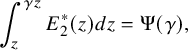 $$ \begin{align*} \int_{z}^{\gamma z} E_2^\ast(z) dz= \Psi(\gamma), \end{align*} $$
where
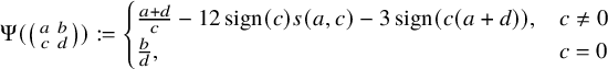
is the Rademacher symbol with
 $$ \begin{align*}s(a,c):=\sum_{n=1}^{ c } (\!(\tfrac{n}{c})\!)(\!(\tfrac{na}{c})\!),\end{align*} $$
the classical Dedekind sum with
 $$ \begin{align*}(\!(x)\!)=\begin{cases}x-\lfloor x\rfloor-1/2,& x\notin \mathbb{Z}\\ 0,& x\in \mathbb{Z}\end{cases}\end{align*} $$
the sawtooth function. Notice that $\Psi (\gamma )$
does not depend on the representative of
$\Psi (\gamma )$
does not depend on the representative of $\gamma \in \mathrm {PSL}_2(\mathbb {Z})$
as should be the case. This implies the following key formula for
$\gamma \in \mathrm {PSL}_2(\mathbb {Z})$
as should be the case. This implies the following key formula for $\gamma \in \Gamma _0(p)$
:
$\gamma \in \Gamma _0(p)$
:
 $$ \begin{align}\langle \{z,\gamma z\}, \omega_{E}(p) \rangle= \frac{\Psi\left(\gamma'\right)- \Psi(\gamma)}{p-1},\end{align} $$
where
with
. Using the trivial bound $\Psi (\gamma )\ll \frac {|a+d|}{ c }+ c $
(for
$\Psi (\gamma )\ll \frac {|a+d|}{ c }+ c $
(for $c> 0$
), we get the following useful estimate:
$c> 0$
), we get the following useful estimate:

Recall the short exact sequence (3.8) above. A Hecke-equivariant splitting is given by mapping $1\in \mathbb {R}$
to the Eisenstein class
$1\in \mathbb {R}$
to the Eisenstein class $\omega _{E}(p)=E_{2,p}(z)dz$
(this fits into a general framework due to Franke [Reference FrankeFra98]). This defines an isomorphism
$\omega _{E}(p)=E_{2,p}(z)dz$
(this fits into a general framework due to Franke [Reference FrankeFra98]). This defines an isomorphism
 $$ \begin{align}H^1(Y_0(p),\mathbb{R})\cong H^1(X_0(p),\mathbb{R})\oplus \mathbb{R} \omega_{E}(p),\end{align} $$
and we will denote the projection to the ‘cuspidal subspace’ (which we will identify with $H^1(X_0(p),\mathbb {R})$
) with respect to this splitting by
$H^1(X_0(p),\mathbb {R})$
) with respect to this splitting by
 $$ \begin{align} \mathbb{P}_{\mathrm{cusp}}:H^1(Y_0(p),\mathbb{R})\rightarrow H^1(X_0(p),\mathbb{R})\subset H^1(Y_0(p),\mathbb{R}), \end{align} $$
which is explicitly given by
 $$ \begin{align*} \mathbb{P}_{\mathrm{cusp}} \omega= \omega- \langle v_{E}(p),\omega\rangle\omega_{E}(p), \end{align*} $$
where $v_{E}(p), \omega _{E}(p)$
are the Eisenstein classes defined above.
$v_{E}(p), \omega _{E}(p)$
are the Eisenstein classes defined above.
4 Background on Fuchsian groups
In this section, we will review some useful facts regarding the geometry of fundamental polygons of Fuchsian groups. We will refer to [Reference BeardonBea83, Section 9] for an in-depth treatment.
4.1 Fundamental polygons
Let $\Gamma \subset \mathrm {PSL}_2(\mathbb {R})$
be a Fuchsian subgroup of the first kind (i.e., a discrete and cofinite subgroup of
$\Gamma \subset \mathrm {PSL}_2(\mathbb {R})$
be a Fuchsian subgroup of the first kind (i.e., a discrete and cofinite subgroup of $\mathrm {PSL}_2(\mathbb {R})$
). A fundamental domain for
$\mathrm {PSL}_2(\mathbb {R})$
). A fundamental domain for $\Gamma $
is a locally finite domain
$\Gamma $
is a locally finite domain $\mathcal {F}\subset \mathbb {H}$
such that
$\mathcal {F}\subset \mathbb {H}$
such that
-
1. For any $z\in \mathbb {H}$
, we have
$\gamma z\in \overline {\mathcal {F}}$
for some
$\gamma \in \Gamma $
.
$z\in \mathbb {H}$
, we have
$\gamma z\in \overline {\mathcal {F}}$
for some
$\gamma \in \Gamma $
. -
2. If
$z_1,z_2\in \overline {\mathcal {F}}$
are
$\Gamma $
-equivalent, then
$z_1=z_2$
or
$z_1,z_2\in \partial \mathcal {F}$
.


We say that $\mathcal {F}$
is a fundamental polygon for
$\mathcal {F}$
is a fundamental polygon for $\Gamma $
if
$\Gamma $
if $\mathcal {F}$
is furthermore (hyperbolically) convex with a piecewise geodesic boundary. We define a side of
$\mathcal {F}$
is furthermore (hyperbolically) convex with a piecewise geodesic boundary. We define a side of $\mathcal {F}$
as a nonempty subset of the shape
$\mathcal {F}$
as a nonempty subset of the shape $\gamma \overline {\mathcal {F}}\cap \overline {\mathcal {F}}$
with
$\gamma \overline {\mathcal {F}}\cap \overline {\mathcal {F}}$
with $ \mathrm {Id}\neq \gamma \in \Gamma $
. We define a vertex of
$ \mathrm {Id}\neq \gamma \in \Gamma $
. We define a vertex of $\mathcal {F}$
as a non-empty subset of the shape
$\mathcal {F}$
as a non-empty subset of the shape $\gamma _1 \overline {\mathcal {F}}\cap \gamma _2 \overline {\mathcal {F}} \cap \overline {\mathcal {F}}$
with
$\gamma _1 \overline {\mathcal {F}}\cap \gamma _2 \overline {\mathcal {F}} \cap \overline {\mathcal {F}}$
with $ \mathrm {Id},\gamma _1,\gamma _2\in \Gamma $
pairwise distinct. It can be shown that a fundamental polygon
$ \mathrm {Id},\gamma _1,\gamma _2\in \Gamma $
pairwise distinct. It can be shown that a fundamental polygon $\mathcal {F}$
has an even number of sides which are pairwise
$\mathcal {F}$
has an even number of sides which are pairwise $\Gamma $
-equivalent, and
$\Gamma $
-equivalent, and $\Gamma \mathcal {F}$
gives a tessellation of
$\Gamma \mathcal {F}$
gives a tessellation of $\mathbb {H}$
. The set of elements identifying sides of
$\mathbb {H}$
. The set of elements identifying sides of $\mathcal {F}$
are called the side pairing transformations associated to
$\mathcal {F}$
are called the side pairing transformations associated to $\mathcal {F}$
which we denote by
$\mathcal {F}$
which we denote by $\mathcal {S}(\mathcal {F})\subset \Gamma $
(which formally is a multiset if there are order two elements in
$\mathcal {S}(\mathcal {F})\subset \Gamma $
(which formally is a multiset if there are order two elements in $\Gamma $
). Given a side L of
$\Gamma $
). Given a side L of $\mathcal {F}$
we refer to the side pairing transformation associated to the side L as the element
$\mathcal {F}$
we refer to the side pairing transformation associated to the side L as the element $\sigma \in \mathcal {S}(\mathcal {F})$
such that
$\sigma \in \mathcal {S}(\mathcal {F})$
such that $\sigma ^{-1}L$
is also a side of
$\sigma ^{-1}L$
is also a side of $\mathcal {F}$
. Similarly we say that
$\mathcal {F}$
. Similarly we say that $\sigma $
is the side pairing transformation associated to the side
$\sigma $
is the side pairing transformation associated to the side $\gamma L$
of the translate
$\gamma L$
of the translate $\gamma \mathcal {F}$
for each
$\gamma \mathcal {F}$
for each $\gamma \in \Gamma $
.
$\gamma \in \Gamma $
.
It is known that $\mathcal {S}(\mathcal {F})$
generates
$\mathcal {S}(\mathcal {F})$
generates $\Gamma $
for any fundamental polygon
$\Gamma $
for any fundamental polygon $\mathcal {F}$
, and it is a fundamental fact that one can understand the relation between the elements of
$\mathcal {F}$
, and it is a fundamental fact that one can understand the relation between the elements of $\mathcal {S}(\mathcal {F})$
from the geometry of a fundamental polygon and vice versa (see Lemma 4.3). A simple but key incarnation is the following.
$\mathcal {S}(\mathcal {F})$
from the geometry of a fundamental polygon and vice versa (see Lemma 4.3). A simple but key incarnation is the following.
Proposition 4.1. Let $\mathcal {F}$
be a fundamental polygon for a discrete and co-finite subgroup
$\mathcal {F}$
be a fundamental polygon for a discrete and co-finite subgroup $\Gamma \subset \mathrm {PSL}_2(\mathbb {R})$
. Consider a sequence of consecutive
$\Gamma \subset \mathrm {PSL}_2(\mathbb {R})$
. Consider a sequence of consecutive $\Gamma $
-translates of
$\Gamma $
-translates of $\mathcal {F}$
:
$\mathcal {F}$
:
 $$ \begin{align*} \mathcal{F},\gamma_1 \mathcal{F},\ldots, \gamma_n \mathcal{F}. \end{align*} $$
Then
 $$ \begin{align*}\gamma_n=\sigma_1\sigma_2\cdots \sigma_n, \end{align*} $$
where $\sigma _i\in \mathcal {S}(\mathcal {F})$
denotes the side pairing transformation associated to the side shared between
$\sigma _i\in \mathcal {S}(\mathcal {F})$
denotes the side pairing transformation associated to the side shared between $\gamma _{i-1} \mathcal {F}$
and
$\gamma _{i-1} \mathcal {F}$
and $\gamma _{i} \mathcal {F}$
(here, we put
$\gamma _{i} \mathcal {F}$
(here, we put $\gamma _0=\mathrm {Id}$
).
$\gamma _0=\mathrm {Id}$
).
Proof. Note that the side of $\mathcal {F}$
shared with
$\mathcal {F}$
shared with $\gamma _1 \mathcal {F}$
will exactly have associated
$\gamma _1 \mathcal {F}$
will exactly have associated $\sigma _1=\gamma _1\in \mathcal {S}(\mathcal {F})$
. Now if the side shared between
$\sigma _1=\gamma _1\in \mathcal {S}(\mathcal {F})$
. Now if the side shared between $\gamma _1 \mathcal {F}$
and
$\gamma _1 \mathcal {F}$
and $\gamma _2 \mathcal {F}$
has associated
$\gamma _2 \mathcal {F}$
has associated $\sigma _2\in \mathcal {S}(\mathcal {F})$
, then we have
$\sigma _2\in \mathcal {S}(\mathcal {F})$
, then we have
 $$ \begin{align*}\gamma_2\mathcal{F}=(\sigma_1\sigma_2\sigma_1^{-1})(\sigma_1 \mathcal{F})=\sigma_1 \sigma_2 \mathcal{F}. \end{align*} $$
Continuing like this, we get
 $$ \begin{align*} \gamma_n\mathcal{F}=\sigma_1 \cdots \sigma_n \mathcal{F}, \end{align*} $$
and since $\gamma \mathcal {F}=\gamma ' \mathcal {F}$
implies
$\gamma \mathcal {F}=\gamma ' \mathcal {F}$
implies $\gamma =\gamma '\in \Gamma $
by condition (2), we conclude the wanted equality.
$\gamma =\gamma '\in \Gamma $
by condition (2), we conclude the wanted equality.
A first application of Proposition 4.1 is the following slight reformulation.
Corollary 4.2. Let $c:[0,1]\rightarrow \mathbb {H}$
be a continuous, injective curve with
$c:[0,1]\rightarrow \mathbb {H}$
be a continuous, injective curve with $c(0)=z\in \mathcal {F}$
and
$c(0)=z\in \mathcal {F}$
and $c(1)=\gamma z$
for some
$c(1)=\gamma z$
for some $\gamma \in \Gamma $
. Assume that
$\gamma \in \Gamma $
. Assume that $c([0,1])$
does not intersect the set of
$c([0,1])$
does not intersect the set of $\Gamma $
-translates of the vertices of
$\Gamma $
-translates of the vertices of $\mathcal {F}$
. Then one can code the element
$\mathcal {F}$
. Then one can code the element $\gamma $
in the following way; let
$\gamma $
in the following way; let $\sigma _1,\ldots , \sigma _n\in \mathcal {S}(\mathcal {F})$
be the (ordered) sequence of side pairing transformations associated to the intersection between the curve c and
$\sigma _1,\ldots , \sigma _n\in \mathcal {S}(\mathcal {F})$
be the (ordered) sequence of side pairing transformations associated to the intersection between the curve c and $\Gamma $
-translates of the sides of
$\Gamma $
-translates of the sides of $\mathcal {F}$
. Then one has
$\mathcal {F}$
. Then one has
 $$ \begin{align*} \gamma=\sigma_1\cdots\sigma_n. \end{align*} $$
When $c([0,1])$
is a closed geodesic (when projected to
$c([0,1])$
is a closed geodesic (when projected to $\Gamma \backslash \mathbb {H}$
), this is known as geometric coding of geodesics (see [Reference KatokKat96] for a nice treatment).
$\Gamma \backslash \mathbb {H}$
), this is known as geometric coding of geodesics (see [Reference KatokKat96] for a nice treatment).
As a second consequence, we note that if the sequence of translates ‘loops around’, meaning that ${\gamma _n=1}$
, then one obtains a relation between the side pairing transformations
${\gamma _n=1}$
, then one obtains a relation between the side pairing transformations $S(\Gamma )$
. This yields immediately that if two sides of
$S(\Gamma )$
. This yields immediately that if two sides of $\mathcal {F}$
are paired, then the associated elements in
$\mathcal {F}$
are paired, then the associated elements in $\mathcal {S}(\mathcal {F})$
are inverses. We call these the inverse relations of
$\mathcal {S}(\mathcal {F})$
are inverses. We call these the inverse relations of $\mathcal {F}$
. We also get relations by looping around the vertices of
$\mathcal {F}$
. We also get relations by looping around the vertices of $\mathcal {F}$
which we will now make precise. Observe that the embedding
$\mathcal {F}$
which we will now make precise. Observe that the embedding $\mathcal {F}\subset \mathbb {H}$
defines an orientation on the boundary
$\mathcal {F}\subset \mathbb {H}$
defines an orientation on the boundary $\partial \mathcal {F}$
. Let
$\partial \mathcal {F}$
. Let $L_1$
be a side of
$L_1$
be a side of $\mathcal {F}$
with leftmost (wrt. the orientation) vertex
$\mathcal {F}$
with leftmost (wrt. the orientation) vertex $v_1$
and let
$v_1$
and let $\sigma _1\in \mathcal {S}(\mathcal {F})$
be the associated side pairing transformation. Let
$\sigma _1\in \mathcal {S}(\mathcal {F})$
be the associated side pairing transformation. Let $L_2$
be the side of
$L_2$
be the side of $\mathcal {F}$
different from
$\mathcal {F}$
different from $\sigma _1^{-1} L_1$
containing the vertex
$\sigma _1^{-1} L_1$
containing the vertex $v_2=\sigma _1^{-1} v$
and let
$v_2=\sigma _1^{-1} v$
and let $\sigma _2\in \mathcal {S}(\mathcal {F})$
be the associated side pairing transformation. Continuing like this yields a periodic sequence of pairs
$\sigma _2\in \mathcal {S}(\mathcal {F})$
be the associated side pairing transformation. Continuing like this yields a periodic sequence of pairs
 $$ \begin{align*} (L_1,v_1), (L_2,v_2),\ldots, \end{align*} $$
with minimal period $m\geq 1$
, say, which we call a cycle of
$m\geq 1$
, say, which we call a cycle of $\mathcal {F}$
. It is now clear that
$\mathcal {F}$
. It is now clear that $\sigma _1\sigma _2\ldots \sigma _m$
fixes
$\sigma _1\sigma _2\ldots \sigma _m$
fixes $v_1$
. Thus, if we put
$v_1$
. Thus, if we put $\nu =|\Gamma _{v_1}|$
(i.e., the size of the stabilizer of
$\nu =|\Gamma _{v_1}|$
(i.e., the size of the stabilizer of $v_1$
inside
$v_1$
inside $\Gamma $
), then we get the following relation on the side pairing transformations:
$\Gamma $
), then we get the following relation on the side pairing transformations:
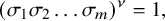 $$ \begin{align*} (\sigma_1\sigma_2\ldots \sigma_m)^\nu=1, \end{align*} $$
where if $\nu =\infty $
(i.e.,
$\nu =\infty $
(i.e., $v_1$
is a boundary vertex), this is understood as the empty relation. Notice that the relation does not depend on the choice of starting point
$v_1$
is a boundary vertex), this is understood as the empty relation. Notice that the relation does not depend on the choice of starting point $(L_1,v_1)$
. We call these the cycle relations of
$(L_1,v_1)$
. We call these the cycle relations of $\mathcal {F}$
, and we have the following key theorem of Poincaré; see [Reference MaskitMas71] for a proof.
$\mathcal {F}$
, and we have the following key theorem of Poincaré; see [Reference MaskitMas71] for a proof.
Lemma 4.3 (Poincaré’s Theorem)
The side pairing transformations $\mathcal {S}(\mathcal {F})$
generate
$\mathcal {S}(\mathcal {F})$
generate $\Gamma $
, and the inverse and cycle relations give a complete set of relations for
$\Gamma $
, and the inverse and cycle relations give a complete set of relations for $\mathcal {S}(\mathcal {F})$
.
$\mathcal {S}(\mathcal {F})$
.
Secondly, it is clear that each side appears in exactly one cycle. Thus, we obtain the following useful fact.
Lemma 4.4 (cf. Lemma 5.3 of [Reference VoightVoi09])
Each side pairing transformation appears exactly once in a cycle relation.
4.1.1 Bounding coordinates of side pairing transformations
Now we consider the image of the inverse and cycle relations when mapped to $V_p$
under the composition of maps:
$V_p$
under the composition of maps:
 $$ \begin{align*}\Gamma_0(p)\twoheadrightarrow \Gamma_0(p)^{\mathrm{ab}}\twoheadrightarrow H_1(Y_0(p),\mathbb{Z})\hookrightarrow V_p=H_1(Y_0(p),\mathbb{R})\cong \mathbb{R}^{2g+1}.\end{align*} $$
Notice that since $V_p$
is torsion-free, we can divide the relations by
$V_p$
is torsion-free, we can divide the relations by $\nu $
so that all coefficients in the relations are contained in
$\nu $
so that all coefficients in the relations are contained in $\{-1,0,1\}$
. By killing the inverse relations, this yields a system of linear relations with a variable for each pair
$\{-1,0,1\}$
. By killing the inverse relations, this yields a system of linear relations with a variable for each pair $\{\sigma ,\sigma ^{-1}\}\subset \mathcal {S}(\mathcal {F})$
of side pairing transformations so that each such variable appears once with positive and once with negative sign (which follows from Lemma 4.4).
$\{\sigma ,\sigma ^{-1}\}\subset \mathcal {S}(\mathcal {F})$
of side pairing transformations so that each such variable appears once with positive and once with negative sign (which follows from Lemma 4.4).
Let $B=\{v_0,\ldots , v_{2g}\}\subset V_p$
be a basis of the real homology corresponding to side pairing transformations
$B=\{v_0,\ldots , v_{2g}\}\subset V_p$
be a basis of the real homology corresponding to side pairing transformations $\sigma \in \mathcal {S}(\mathcal {F})$
under the surjection (3.5). Combining the cycle relations with the choice of B gives rise to a system of linear equations in
$\sigma \in \mathcal {S}(\mathcal {F})$
under the surjection (3.5). Combining the cycle relations with the choice of B gives rise to a system of linear equations in $V_p$
:
$V_p$
:
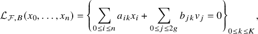 $$ \begin{align*}\mathcal{L}_{\mathcal{F},B}(x_0,\ldots, x_n)= \left\{ \sum_{0\leq i\leq n} a_{ik}x_i+\sum_{0\leq j\leq 2g} b_{jk}v_j=0 \right\}_{0\leq k \leq K},\end{align*} $$
where $x_0,\ldots , x_n$
are variables, one for each pair
$x_0,\ldots , x_n$
are variables, one for each pair $\{\sigma ,\sigma ^{-1}\}\subset \mathcal {S}(\mathcal {F})$
not corresponding to an element of B. Lemmata 4.3 and 4.4 translate to two key properties:
$\{\sigma ,\sigma ^{-1}\}\subset \mathcal {S}(\mathcal {F})$
not corresponding to an element of B. Lemmata 4.3 and 4.4 translate to two key properties:
-
1.
$\mathcal {L}_{\mathcal {F},B}$
has exactly one solution
$(x_0,\ldots , x_n)\in (V_p)^{n+1}$
. -
2. For any subset
$A\subset \{0,\ldots , K\}$
, and any indices
$0\leq i\leq n,0\leq j\leq 2g$
, we have
$$ \begin{align*} \sum_{k\in A}a_{ik},\, \sum_{k\in A}b_{jk} \in \{-1,0,1\}. \end{align*} $$


We have the following general result about such systems of linear equations.
Lemma 4.5. Let
 $$ \begin{align*}\mathcal{L}(x_0,\ldots, x_n)= \left\{ \sum_{0\leq i\leq n} a_{ik}x_i+\sum_{0\leq j\leq 2g} b_{jk}v_j=0 \right\}_{0\leq k \leq K}\end{align*} $$
be a system of linear equations in $V_p$
satisfying (1) and (2).
$V_p$
satisfying (1) and (2).
Then the unique solution $(x_0,\ldots , x_n)\in (V_p)^{n+1}$
satisfies
$(x_0,\ldots , x_n)\in (V_p)^{n+1}$
satisfies
 $$ \begin{align}x_i=\sum_{0\leq j\leq 2g} c_{ij} v_j,\quad c_{ij}\in \{-1,0,1\},\end{align} $$
for all $0\leq i\leq n$
.
$0\leq i\leq n$
.
Proof. We proceed by induction on $K+1\geq 0$
(i.e., the number of equations). If
$K+1\geq 0$
(i.e., the number of equations). If $K+1=0$
, then there is nothing to prove. Now assume the claim is known for systems of
$K+1=0$
, then there is nothing to prove. Now assume the claim is known for systems of $K'<K+1$
equations. We start by making the following reductions. We may assume that all equations contain a variable (i.e.,
$K'<K+1$
equations. We start by making the following reductions. We may assume that all equations contain a variable (i.e., $\forall k \exists i:a_{ik}\neq 0$
), since otherwise we can remove such an equation. Furthermore, we may assume that there are some variables appearing exactly once (i.e.,
$\forall k \exists i:a_{ik}\neq 0$
), since otherwise we can remove such an equation. Furthermore, we may assume that there are some variables appearing exactly once (i.e., $\exists i : |\{k: a_{ik}\neq 0\}|=1$
). If this is not the case, then by (1) and (2) every variable appears exactly twice with coefficients
$\exists i : |\{k: a_{ik}\neq 0\}|=1$
). If this is not the case, then by (1) and (2) every variable appears exactly twice with coefficients $\pm 1$
, respectively. This means that the equation obtained by adding all of the equations in
$\pm 1$
, respectively. This means that the equation obtained by adding all of the equations in $\mathcal {L}(x_0,\ldots , x_n)$
has to be trivial. Thus, by removing any equation, we obtain an equivalent system with K equations, and we are done by the induction hypothesis.
$\mathcal {L}(x_0,\ldots , x_n)$
has to be trivial. Thus, by removing any equation, we obtain an equivalent system with K equations, and we are done by the induction hypothesis.
The key observation is that there is always an equation with exactly one variable appearing (i.e., $\exists k : |\{i: a_{ik}\neq 0\}|=1$
). If not, then since every variable appears at most twice and there is one variable appearing once (by the above reductions) we have a system of linear equations with more variables than equations. Thus, the number of solutions
$\exists k : |\{i: a_{ik}\neq 0\}|=1$
). If not, then since every variable appears at most twice and there is one variable appearing once (by the above reductions) we have a system of linear equations with more variables than equations. Thus, the number of solutions $(x_0,\ldots , x_n)\in (V_p)^{n+1}$
is either
$(x_0,\ldots , x_n)\in (V_p)^{n+1}$
is either $0$
or
$0$
or $\infty $
, which contradicts (1). Let
$\infty $
, which contradicts (1). Let $x_i$
be the only variable appearing in some equation. Then this equation determines
$x_i$
be the only variable appearing in some equation. Then this equation determines $x_i$
, which by (2) satisfies (4.1). Now if
$x_i$
, which by (2) satisfies (4.1). Now if $-x_i$
does not appear, we are done by the induction hypothesis. Otherwise, we add the equation containing
$-x_i$
does not appear, we are done by the induction hypothesis. Otherwise, we add the equation containing $x_i$
to the one containing
$x_i$
to the one containing $-x_i$
which gives a system of K linear equations again satisfying (1) and (2). Thus, the claim follows from the induction hypothesis.
$-x_i$
which gives a system of K linear equations again satisfying (1) and (2). Thus, the claim follows from the induction hypothesis.
Corollary 4.6. Let $\Gamma $
be a Fuchsian group with a fundamental polygon
$\Gamma $
be a Fuchsian group with a fundamental polygon $\mathcal {F}$
, and let B be a basis for
$\mathcal {F}$
, and let B be a basis for $H_1(\Gamma \backslash \mathbb {H}, \mathbb {R})$
consisting of classes of the form
$H_1(\Gamma \backslash \mathbb {H}, \mathbb {R})$
consisting of classes of the form $\{z,\sigma z\}$
with
$\{z,\sigma z\}$
with $\sigma \in \mathcal {S}(\mathcal {F})$
and
$\sigma \in \mathcal {S}(\mathcal {F})$
and $z\in \mathbb {H}$
.
$z\in \mathbb {H}$
.
Then we have for any $\sigma \in \mathcal {S}(\mathcal {F})$
,
$\sigma \in \mathcal {S}(\mathcal {F})$
, $z\in \mathbb {H}$
and
$z\in \mathbb {H}$
and $\omega \in B^{\ast }$
that
$\omega \in B^{\ast }$
that
 $$ \begin{align*} |\langle \{z, \sigma z\}, \omega \rangle|\leq 1.\end{align*} $$
Proof. Observe that if the variable $x_i$
corresponds to
$x_i$
corresponds to $\{\sigma ,\sigma ^{-1}\}\in \mathcal {S}(\mathcal {F})$
, then the numbers
$\{\sigma ,\sigma ^{-1}\}\in \mathcal {S}(\mathcal {F})$
, then the numbers
 $$ \begin{align*} (\langle \{ z, \sigma z\}, \omega \rangle)_{\omega\in B^{\ast}} \end{align*} $$
are exactly the coordinates of either $x_i$
or
$x_i$
or $-x_i$
in the basis B where
$-x_i$
in the basis B where $(x_0,\ldots , x_n)\in (V_p)^{n+1}$
is the unique solution to
$(x_0,\ldots , x_n)\in (V_p)^{n+1}$
is the unique solution to $\mathcal {L}_{\mathcal {F},B}$
. Now the result follows directly from Lemma 4.5.
$\mathcal {L}_{\mathcal {F},B}$
. Now the result follows directly from Lemma 4.5.
4.2 Zagier’s fundamental polygon
We will now consider a fundamental polygon for $\Gamma _0(p)$
introduced by Zagier [Reference ZagierZag85, Section 3] which will give rise to a set of natural bases for the homology. The following is a fundamental polygon for
$\Gamma _0(p)$
introduced by Zagier [Reference ZagierZag85, Section 3] which will give rise to a set of natural bases for the homology. The following is a fundamental polygon for $\Gamma _0(p)$
:
$\Gamma _0(p)$
:
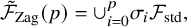 $$ \begin{align*} \tilde{\mathcal{F}}_{\mathrm{Zag}}(p)=\cup_{i=0}^{p} \sigma_i \mathcal{F}_{\mathrm{std}},\end{align*} $$
where
for $0\leq i <p$
and
$0\leq i <p$
and
, and
 $$ \begin{align}\mathcal{F}_{\mathrm{std}}:=\{z\in \mathbb{H}: |\operatorname{Re} z|<1/2, |z|>1\}\end{align} $$
is the standard fundamental polygon for $\mathrm {PSL}_2(\mathbb {Z})$
. This gives rise to the side pairing transformation set
$\mathrm {PSL}_2(\mathbb {Z})$
. This gives rise to the side pairing transformation set
where $0<a^*<p$
is such that
$0<a^*<p$
is such that $aa^*\equiv -1 \ \mathrm {mod}\ p$
. Recall that
$aa^*\equiv -1 \ \mathrm {mod}\ p$
. Recall that $\Gamma _0(p)$
is normalized by the matrix
$\Gamma _0(p)$
is normalized by the matrix
, which implies that also $\mathcal {F}_{\mathrm {Zag}}(p):=W_{p} \tilde {\mathcal {F}}_{\mathrm {Zag}}(p)$
is a fundamental polygon for
$\mathcal {F}_{\mathrm {Zag}}(p):=W_{p} \tilde {\mathcal {F}}_{\mathrm {Zag}}(p)$
is a fundamental polygon for $\Gamma _0(p)$
with side pairing transformations given by
$\Gamma _0(p)$
with side pairing transformations given by
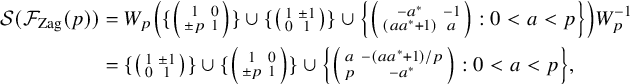
which, by Lemma 4.3, generate $\Gamma _0(p)$
(as claimed in the introduction). Both of these fundamental polygons have the nice property that all cuspidal sides (i.e., sides containing a cusp) are paired by a parabolic element of
$\Gamma _0(p)$
(as claimed in the introduction). Both of these fundamental polygons have the nice property that all cuspidal sides (i.e., sides containing a cusp) are paired by a parabolic element of $\Gamma _0(p)$
(which is not the case for all fundamental polygons). The elements of
$\Gamma _0(p)$
(which is not the case for all fundamental polygons). The elements of $\mathcal {S}(\mathcal {F}_{\mathrm {Zag}}(p))$
are minimal in the sense that the archimedean sizes of the entries are as small as one can hope for (
$\mathcal {S}(\mathcal {F}_{\mathrm {Zag}}(p))$
are minimal in the sense that the archimedean sizes of the entries are as small as one can hope for ( $\leq p$
). Explicitly, the fundamental polygon
$\leq p$
). Explicitly, the fundamental polygon $\mathcal {F}_{\mathrm {Zag}}(p)$
has
$\mathcal {F}_{\mathrm {Zag}}(p)$
has $p+3$
vertices: the two cusps
$p+3$
vertices: the two cusps $0$
and
$0$
and $\infty $
as well as
$\infty $
as well as $\frac {2j-1+i\sqrt {3}}{2p}$
for
$\frac {2j-1+i\sqrt {3}}{2p}$
for $0\leq j\leq p$
. We see that the matrix
$0\leq j\leq p$
. We see that the matrix $W_{p}$
takes the hyperbolic triangle with vertices
$W_{p}$
takes the hyperbolic triangle with vertices $ \{\tfrac {-1+i\sqrt {3}}{2p},0,\tfrac {1+i\sqrt {3}}{2p}\}$
to the hyperbolic triangle with vertices
$ \{\tfrac {-1+i\sqrt {3}}{2p},0,\tfrac {1+i\sqrt {3}}{2p}\}$
to the hyperbolic triangle with vertices $\{ \tfrac {-1+i\sqrt {3}}{2},\infty ,\tfrac {1+i\sqrt {3}}{2}\}$
. In particular, the subgroup
$\{ \tfrac {-1+i\sqrt {3}}{2},\infty ,\tfrac {1+i\sqrt {3}}{2}\}$
. In particular, the subgroup $\langle W_{p}, \Gamma _0(p)\rangle \leq \mathrm {PSL}_2(\mathbb {R})$
has a fundamental domain contained in
$\langle W_{p}, \Gamma _0(p)\rangle \leq \mathrm {PSL}_2(\mathbb {R})$
has a fundamental domain contained in
 $$ \begin{align} \{ z\in \mathbb{H} : |\operatorname{Re} z|\leq 1/2, \operatorname{Im} z\geq \sqrt{3}/(2p) \},\end{align} $$
which will be useful later on.
We define the following compatible family of bases of the homology groups.
Definition 4.7. A basic basis of level p is a basis ${B}\subset H_1(Y_0(p),\mathbb {R})$
consisting of elements
${B}\subset H_1(Y_0(p),\mathbb {R})$
consisting of elements $\{z,\sigma z\}$
with
$\{z,\sigma z\}$
with $z\in \mathbb {H}$
and
$z\in \mathbb {H}$
and $\sigma \in \mathcal {S}(\mathcal {F}_{\mathrm {Zag}}(p))$
.
$\sigma \in \mathcal {S}(\mathcal {F}_{\mathrm {Zag}}(p))$
.
4.3 Special fundamental polygons
By the Kurosh subgroup theorem, we know that any subgroup of $\mathrm {PSL}_2(\mathbb {Z})\cong \mathbb {Z}/2\mathbb {Z}\ast \mathbb {Z}/3\mathbb {Z}$
is isomorphic to a free product of a number of copies of
$\mathrm {PSL}_2(\mathbb {Z})\cong \mathbb {Z}/2\mathbb {Z}\ast \mathbb {Z}/3\mathbb {Z}$
is isomorphic to a free product of a number of copies of $\mathbb {Z}/2\mathbb {Z},\mathbb {Z}/3\mathbb {Z}$
and
$\mathbb {Z}/2\mathbb {Z},\mathbb {Z}/3\mathbb {Z}$
and $\mathbb {Z}$
. In particular, a torsion-free Hecke congruence subgroup
$\mathbb {Z}$
. In particular, a torsion-free Hecke congruence subgroup $\Gamma _0(p)$
is a free group on
$\Gamma _0(p)$
is a free group on $k=\mathrm {rank}_{\mathbb {Z}}\, \Gamma _0(p)^{\mathrm {ab}}$
generators. We will now describe an explicit geometric way due to Kulkarni [Reference KulkarniKul91] for constructing a set of independent generators of
$k=\mathrm {rank}_{\mathbb {Z}}\, \Gamma _0(p)^{\mathrm {ab}}$
generators. We will now describe an explicit geometric way due to Kulkarni [Reference KulkarniKul91] for constructing a set of independent generators of $\Gamma _0(p)$
. The starting points are so-called special fundamental polygons of
$\Gamma _0(p)$
. The starting points are so-called special fundamental polygons of $\Gamma _0(p)$
.
$\Gamma _0(p)$
.
Let g be the genus of $Y_0(p)$
, and
$Y_0(p)$
, and $e_2,e_3$
the number of conjugacy classes of subgroups in
$e_2,e_3$
the number of conjugacy classes of subgroups in $\Gamma _0(p)$
of order, respectively,
$\Gamma _0(p)$
of order, respectively, $2$
and
$2$
and $3$
. Following [Reference KulkarniKul91], we define a Farey symbol of level p as a sequence of reduced fractions
$3$
. Following [Reference KulkarniKul91], we define a Farey symbol of level p as a sequence of reduced fractions
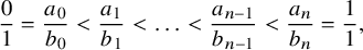 $$ \begin{align*} \frac{0}{1}=\frac{a_{0}}{b_{0}}<\frac{a_1}{b_1}<\ldots<\frac{a_{n-1}}{b_{n-1}}< \frac{a_{n}}{b_{n}}=\frac{1}{1} , \end{align*} $$
with $n=4g+e_2+e_3$
such that
$n=4g+e_2+e_3$
such that $a_{i+1}b_{i}-a_{i}b_{i+1}=1$
for all
$a_{i+1}b_{i}-a_{i}b_{i+1}=1$
for all $1\leq i<n$
. Furthermore (considering below the indices modulo
$1\leq i<n$
. Furthermore (considering below the indices modulo $n+2$
),
$n+2$
),
-
○ there are
$e_2$
even indices i such that
$$ \begin{align*} b_i^2+b_{i+1}^2 \equiv 0\ \mathrm{mod}\ p, \end{align*} $$
-
○ there are
$e_3$
odd indices i such that
$$ \begin{align*} b_i^2+b_ib_{i+1}+b_{i+1}^2 \equiv 0\ \mathrm{mod}\ p, \end{align*} $$
-
○ for the remaining
$4g$
free indices, there is a pairing
$i\leftrightarrow i^\ast $
satisfying
$$ \begin{align*} b_ib_{i^\ast}+b_{i+1}b_{i^\ast+1}\equiv 0\ \mathrm{mod}\ p. \end{align*} $$


Such a symbol always exists, and one can even find one which is symmetric around $1/2$
[Reference KulkarniKul91, Section 13]. Dooms–Jesper–Konolalov [Reference Dooms, Jespers and KonovalovDJK10] have described an algorithm for determining Farey symbols of a general level.
$1/2$
[Reference KulkarniKul91, Section 13]. Dooms–Jesper–Konolalov [Reference Dooms, Jespers and KonovalovDJK10] have described an algorithm for determining Farey symbols of a general level.
Consider the polygon $\mathcal {P}(p)$
with vertices at
$\mathcal {P}(p)$
with vertices at $\infty $
, at the fractions of the Farey symbol, at the midpoint of the geodesic circle connecting
$\infty $
, at the fractions of the Farey symbol, at the midpoint of the geodesic circle connecting $a_i/b_i$
and
$a_i/b_i$
and $a_{i+1}/b_{i+1}$
for i an even index, and for an odd index i at the
$a_{i+1}/b_{i+1}$
for i an even index, and for an odd index i at the $\mathrm {PGL}_2(\mathbb {Z})$
-translate of
$\mathrm {PGL}_2(\mathbb {Z})$
-translate of $\frac {1+i\sqrt {3}}{2}$
lying between
$\frac {1+i\sqrt {3}}{2}$
lying between $a_i/b_i$
and
$a_i/b_i$
and $a_{i+1}/b_{i+1}$
(for details see [Reference KulkarniKul91, Section 2]). Note that
$a_{i+1}/b_{i+1}$
(for details see [Reference KulkarniKul91, Section 2]). Note that $\mathcal {P}(p)$
consists of
$\mathcal {P}(p)$
consists of $\mathrm {PGL}_2(\mathbb {Z})$
-translates of
$\mathrm {PGL}_2(\mathbb {Z})$
-translates of
 $$ \begin{align}\mathcal{F}^+:=\{z\in \mathbb{H}: 0<\operatorname{Re} z<1/2, |z|>1\}. \end{align} $$
The map $\ast $
defines a side pairing transformation on this polygon by identifying the half circle connecting
$\ast $
defines a side pairing transformation on this polygon by identifying the half circle connecting $\frac {a_{i}}{b_{i}},\frac {a_{i+1}}{b_{i+1}}$
and the one connecting
$\frac {a_{i}}{b_{i}},\frac {a_{i+1}}{b_{i+1}}$
and the one connecting $\frac {a_{i^\ast +1}}{b_{i^\ast +1}},\frac {a_{i^\ast }}{b_{i^\ast }}$
, as well as identifying the vertical sides of
$\frac {a_{i^\ast +1}}{b_{i^\ast +1}},\frac {a_{i^\ast }}{b_{i^\ast }}$
, as well as identifying the vertical sides of $\mathcal {P}(p)$
and the elliptic sides. By Poincaré’s theorem,
$\mathcal {P}(p)$
and the elliptic sides. By Poincaré’s theorem, $\mathcal {P}(p)$
together with this pairing defines a subgroup of
$\mathcal {P}(p)$
together with this pairing defines a subgroup of $\mathrm {PSL}_2(\mathbb {R})$
which can be shown to be equal to
$\mathrm {PSL}_2(\mathbb {R})$
which can be shown to be equal to $\Gamma _0(p)$
. Furthermore, since
$\Gamma _0(p)$
. Furthermore, since $\mathcal {P}(p)$
has a minimal number of sides, it follows that an independent set of generators of
$\mathcal {P}(p)$
has a minimal number of sides, it follows that an independent set of generators of $\Gamma _0(p)$
is given by the matrices which map between the sides identified by the pairing induced from
$\Gamma _0(p)$
is given by the matrices which map between the sides identified by the pairing induced from $\ast $
. These matrices are explicitly given by (see [Reference KulkarniKul91, Theorem 6.1])
$\ast $
. These matrices are explicitly given by (see [Reference KulkarniKul91, Theorem 6.1])
and the $e_2$
matrices of order
$e_2$
matrices of order $2$
and
$2$
and $e_3$
matrices of order
$e_3$
matrices of order $3$
$3$
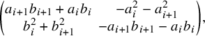 $$ \begin{align} &\begin{pmatrix} a_{i+1}b_{i+1}+a_{i}b_i & -a_i^2-a_{i+1}^2 \\ b_i^2+b_{i+1}^2 & -a_{i+1}b_{i+1}-a_{i}b_{i}\end{pmatrix},\qquad\qquad\quad\qquad \end{align} $$
 $$ \begin{align} &\begin{pmatrix} a_{i+1}b_{i+1}+a_{i}b_{i+1}+a_{i}b_i & -a_i^2-a_ia_{i+1}-a_{i+1}^2 \\ b_i^2+b_ib_{i+1}+b_{i+1}^2 & -a_{i+1}b_{i+1}-a_{i+1}b_i-a_{i}b_{i}\end{pmatrix}, \end{align} $$
together with the $2g$
hyperbolic matrices
$2g$
hyperbolic matrices
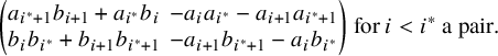 $$ \begin{align} \begin{pmatrix} a_{i^\ast+1}b_{i+1}+a_{i^\ast}b_i & -a_ia_{i^\ast}-a_{i+1}a_{i^\ast+1} \\ b_ib_{i^\ast}+b_{i+1}b_{i^\ast+1} & -a_{i+1}b_{i^\ast+1}-a_{i}b_{i^\ast}\end{pmatrix} \text{ for } i<i^\ast \text{ a pair}. \end{align} $$
Observe that the $2g$
hyperbolic matrices above, together with T, define a basis for
$2g$
hyperbolic matrices above, together with T, define a basis for $H_1(Y_0(p),\mathbb {R})$
under the map (3.5). Recently, Doan–Kim–Lang–Tan [Reference Doan, Kim, Lang and TanDKLP22] have shown that one can find minimal special fundamental polygons
$H_1(Y_0(p),\mathbb {R})$
under the map (3.5). Recently, Doan–Kim–Lang–Tan [Reference Doan, Kim, Lang and TanDKLP22] have shown that one can find minimal special fundamental polygons $\mathcal {P}_{\mathrm {min}}(p)$
, meaning that we have
$\mathcal {P}_{\mathrm {min}}(p)$
, meaning that we have
 $$ \begin{align*} b_ib_{i^\ast}+b_{i+1}b_{i^\ast+1}=p, \quad 0\leq i\leq n, \end{align*} $$
which implies that, in fact, $\mathcal {S}(\mathcal {P}_{\mathrm {min}}(p))\subset \mathcal {S}(\mathcal {F}_{\mathrm {Zag}}(p))$
.
$\mathcal {S}(\mathcal {P}_{\mathrm {min}}(p))\subset \mathcal {S}(\mathcal {F}_{\mathrm {Zag}}(p))$
.
5 Proof of Theorem 1.1
In this section, we will prove the following statement which implies our first main result.
Theorem 5.1. Fix a prime p and $\delta \in (0,\tfrac {1}{2114})$
. Consider a real quadratic field K of discriminant
$\delta \in (0,\tfrac {1}{2114})$
. Consider a real quadratic field K of discriminant $d_K $
such that p splits in K with
$d_K $
such that p splits in K with $p\mathcal {O}_K=\mathfrak {p}_1\mathfrak {p}_2$
. Consider a subgroup
$p\mathcal {O}_K=\mathfrak {p}_1\mathfrak {p}_2$
. Consider a subgroup $H\leq \mathrm {Cl}_K^+$
with
$H\leq \mathrm {Cl}_K^+$
with $\mathfrak {p}_1 \notin H$
and
$\mathfrak {p}_1 \notin H$
and $J=(\sqrt {d_K})\notin H$
.
$J=(\sqrt {d_K})\notin H$
.
Then for any $\omega \in H^1(Y_0(p), \mathbb {R})$
, we have as
$\omega \in H^1(Y_0(p), \mathbb {R})$
, we have as $d_K \rightarrow \infty $
 $$ \begin{align} \frac{\sum_{A\in H} \langle [\mathcal{C}_{A}(p)], \omega \rangle}{|\sum_{A\in H} \langle [\mathcal{C}_{A}(p)], \omega_{E}(p) \rangle|}= -\langle v_{E}(p), \omega\rangle+O_\omega(d_K^{-\delta}), \end{align} $$
where $\langle \cdot , \cdot \rangle $
denotes the cap product pairing, and
$\langle \cdot , \cdot \rangle $
denotes the cap product pairing, and $v_{E}(p),\omega _{E}(p)$
are the Eisenstein classes in (co)homology defined in (3.16) and (3.19).
$v_{E}(p),\omega _{E}(p)$
are the Eisenstein classes in (co)homology defined in (3.16) and (3.19).
First of all, let us see how Theorem 1.1 follows from this.
Proof of Theorem 1.1 assuming Theorem 5.1
Let B be any basis of $V_p=H_1(Y_0(p),\mathbb {R})$
containing
$V_p=H_1(Y_0(p),\mathbb {R})$
containing $v_E(p)$
and let
$v_E(p)$
and let $ B^{\ast }$
denote the dual basis of
$ B^{\ast }$
denote the dual basis of $H^1(Y_0(p),\mathbb {R})$
with respect to the cap product pairing. Consider the isomorphism
$H^1(Y_0(p),\mathbb {R})$
with respect to the cap product pairing. Consider the isomorphism $V_p\cong \mathbb {R}^{2g+1}$
defined by sending B to the standard basis of
$V_p\cong \mathbb {R}^{2g+1}$
defined by sending B to the standard basis of $\mathbb {R}^{2g+1}$
and denote by
$\mathbb {R}^{2g+1}$
and denote by $|\!|\cdot |\!|=|\!|\cdot |\!|_{B,\infty }$
the norm on
$|\!|\cdot |\!|=|\!|\cdot |\!|_{B,\infty }$
the norm on $V_p$
obtained by pulling back the sup norm with respect to the standard basis of
$V_p$
obtained by pulling back the sup norm with respect to the standard basis of $\mathbb {R}^{2g+1}$
. We will prove the convergence (1.8) which implies Theorem 1.1. By Theorem 5.1, we have for
$\mathbb {R}^{2g+1}$
. We will prove the convergence (1.8) which implies Theorem 1.1. By Theorem 5.1, we have for $d_K$
large enough that
$d_K$
large enough that
 $$ \begin{align} \left|\left|\sum_{A\in H}[\mathcal{C}_{A}(p)]\right|\right|=\max_{\omega \in B^{\ast}} \left|\sum_{A\in H}\langle [\mathcal{C}_{A}(p)], \omega\rangle \right|&= \left| \sum_{A\in H} \langle [\mathcal{C}_{A}(p)], \omega_{E}(p) \rangle \right| \max_{\omega \in B^{\ast}} \left(|\langle v_{E}(p), \omega\rangle |+O_\omega(d_K^{-\delta})\right) \end{align} $$
 $$ \begin{align} \hspace{102pt}= \left| \sum_{A\in H} \langle [\mathcal{C}_{A}(p)], \omega_{E}(p) \rangle \right| (1+O_B(d_K^{-\delta})). \end{align} $$
By the triangle inequality, we conclude that
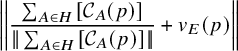 $$ \begin{align} &\!\left|\left|\frac{\sum_{A\in H}[\mathcal{C}_{A}(p)]}{|\!|\sum_{A\in H}[\mathcal{C}_{A}(p)]|\!|} +v_{E}(p) \right|\right| \qquad\qquad\qquad\qquad\qquad\qquad\qquad\qquad\qquad\end{align} $$
 $$ \begin{align} &\leq \left|\left|\frac{\sum_{A\in H}[\mathcal{C}_{A}(p)]}{|\langle \sum_{A\in H} [\mathcal{C}_{A}(p)], \omega_E(p)\rangle|}+v_{E}(p) \right|\right|+ \left| \frac{|\!|\sum_{A\in H}[\mathcal{C}_{A}(p)]|\!|}{|\langle \sum_{A\in H} [\mathcal{C}_{A}(p)], \omega_E(p)\rangle|}-1\right|. \end{align} $$
Finally by (5.3) and Theorem 5.1, the above is bounded by $O_B(d_K^{-\delta })$
, which yields the wanted expression.
$O_B(d_K^{-\delta })$
, which yields the wanted expression.
The rest of this section is occupied with the proof of Theorem 5.1. The idea is to do a change of coordinates to the Hecke basis (3.15) of the real cohomology. Then using formulas due to Hecke and Waldspurger (more precisely, an explicit extension due in this case to Popa [Reference PopaPop08]), we reduce the problem to a question about certain special values of L-functions. Now the result follows upon applying subconvexity bounds (as well as lower bounds for L-functions on the critical line). This is exactly the same proof structure as is used in the automorphic approach to Duke’s Theorem (see, for example, [Reference Michel and VenkateshMV06] and the references therein).
Given $\omega \in H^1(Y_0(p), \mathbb {R})$
, we obtain by expanding in the Hecke basis for homology defined in (3.18) that
$\omega \in H^1(Y_0(p), \mathbb {R})$
, we obtain by expanding in the Hecke basis for homology defined in (3.18) that
 $$ \begin{align*} \langle [\mathcal{C}_{A}(p)], \omega \rangle&=\langle v_{E}(p), \omega \rangle \langle [\mathcal{C}_{A}(p)], \omega_{E}(p) \rangle + \sum_{f\in \mathcal{B}_p, \pm} \langle v_f^{\pm}, \omega\rangle \langle [\mathcal{C}_{A}(p)], \omega_f^{\pm} \rangle. \end{align*} $$
Now we want to average over cosets $CH \subset \mathrm {Cl}_K^+$
for subgroups
$CH \subset \mathrm {Cl}_K^+$
for subgroups $H\leq \mathrm { Cl}_K^+$
of the narrow class group. Using a standard trick from Fourier analysis, we can write
$H\leq \mathrm { Cl}_K^+$
of the narrow class group. Using a standard trick from Fourier analysis, we can write
 $$ \begin{align}\nonumber \sum_{A\in CH} \langle [\mathcal{C}_{A}(p)], \omega \rangle &= \frac{|H|}{|\mathrm{Cl}_K^+|}\sum_{\chi \in \widehat{\mathrm{Cl}_K^+}: \chi_{|H}=1 } \chi(C)\sum_{A\in \mathrm{Cl}_K^+} \langle [\mathcal{C}_{A}(p)], \omega \rangle \overline{\chi}(A) \\[5pt] \nonumber &= \langle v_{E}(p), \omega\rangle \sum_{A\in CH} \langle [\mathcal{C}_{A}(p)], \omega_{E}(p) \rangle \\[5pt] &\quad+\sum_{f\in \mathcal{B}_p, \pm} \langle v_f^{\pm}, \omega\rangle \frac{|H|}{|\mathrm{Cl}_K^+|}\sum_{\chi \in \widehat{\mathrm{Cl}_K^+}: \chi_{|H}=1 } \chi(C)\sum_{A\in \mathrm{Cl}_K^+} \langle [\mathcal{C}_{A}(p)], \omega_f^{\pm} \rangle \overline{\chi}(A). \end{align} $$
The inner sums in the cuspidal contribution are twisted Weyl sums, which we will have to estimate. These sums fits into the framework of toric periods (see, for example, [Reference Einsiedler, Lindenstrauss, Michel and VenkateshELMV11, Section 4]) and they turn out to be related to special values of automorphic L-functions as first proved by Waldspurger [Reference WaldspurgerWal85]. This is exactly the reason why we have changed to the Hecke coordinates.
5.1 The Eisenstein contribution
In order to estimate the Eisenstein contribution, we will rely on the following classical formula of Hecke (see [Reference Duke, Imamoḡlu and TóthDIT18, (68)]):
 $$ \begin{align*} \sum_{A\in \mathrm{ Cl}_K^+} \int_{\mathcal{C}_{A}(p)} E^*_2(z)dz\, \chi(A)= 6(1-\chi(J))L(\chi,0) ,\end{align*} $$
where $E^*_2(z)=E_2(z)-\frac {3}{\pi \operatorname {Im} z}$
(with
$E^*_2(z)=E_2(z)-\frac {3}{\pi \operatorname {Im} z}$
(with $E_2(z)$
defined in (3.17)),
$E_2(z)$
defined in (3.17)), $J=(\sqrt {D})\in \mathrm {Cl}_K^+$
is the different of K and
$J=(\sqrt {D})\in \mathrm {Cl}_K^+$
is the different of K and $L(\chi ,s)$
denotes the (finite part) of the Hecke L-function associated to the narrow class group character
$L(\chi ,s)$
denotes the (finite part) of the Hecke L-function associated to the narrow class group character $\chi $
. Thus, by a change of variable, we get
$\chi $
. Thus, by a change of variable, we get
 $$ \begin{align*} \sum_{A\in \mathrm{Cl}_K^+} \int_{\mathcal{C}_{A}(p)} pE^*_2(pz)dz \, \chi(A)=\sum_{A\in \mathrm{Cl}_K^+} \int_{p\,\mathcal{C}_{A}(p)} E^*_2(z)dz \, \chi(A). \end{align*} $$
We notice by direct computation that $p\,\mathcal {C}_{A}(p)$
(i.e., the dilation of
$p\,\mathcal {C}_{A}(p)$
(i.e., the dilation of $\mathcal {C}_{A}(p)$
by the factor p) is again a closed geodesic as follows. If
$\mathcal {C}_{A}(p)$
by the factor p) is again a closed geodesic as follows. If $\mathcal {C}_{A}(p)$
corresponds to the quadratic form
$\mathcal {C}_{A}(p)$
corresponds to the quadratic form $ax^2+bxy+cy^2$
of discriminant
$ax^2+bxy+cy^2$
of discriminant $d_K $
and level p, then
$d_K $
and level p, then $p\,\mathcal {C}_{A}(p)$
corresponds to
$p\,\mathcal {C}_{A}(p)$
corresponds to $\tfrac {a}{p}x^2+bxy+cpy^2$
(which now might not be of level p). Recall that in Section 3.1 we fixed a residue
$\tfrac {a}{p}x^2+bxy+cpy^2$
(which now might not be of level p). Recall that in Section 3.1 we fixed a residue $r \ \mathrm {mod}\ 2p$
such that
$r \ \mathrm {mod}\ 2p$
such that $r^2\equiv d_K \ \mathrm {mod}\ 4p$
. One can now check by direct computation on ideals that
$r^2\equiv d_K \ \mathrm {mod}\ 4p$
. One can now check by direct computation on ideals that
 $$ \begin{align*} \left(\mathbb{Z} \frac{a}{p} + \mathbb{Z} \frac{b - \sqrt{d_K}}{2}\right) \left(\mathbb{Z} p + \mathbb{Z} \frac{r - \sqrt{d_K}}{2}\right) = \mathbb{Z} a + \mathbb{Z} \frac{b - \sqrt{d_K}}{2} \end{align*} $$
if $a> 0$
, and similarly,
$a> 0$
, and similarly,
 $$ \begin{align*} \left(\mathbb{Z} \left(-\frac{a}{p}\sqrt{d_K}\right) + \mathbb{Z} \frac{d - b\sqrt{d_K}}{2}\right) \left(\mathbb{Z} p + \mathbb{Z} \frac{r - \sqrt{d_K}}{2}\right) = \mathbb{Z} (-a\sqrt{d_K}) + \mathbb{Z} \frac{d - b\sqrt{d_K}}{2} \end{align*} $$
if $a < 0$
. This implies that when projected to the modular curve
$a < 0$
. This implies that when projected to the modular curve $\mathrm {PSL}_2(\mathbb {Z})\backslash \mathbb {H}$
of level
$\mathrm {PSL}_2(\mathbb {Z})\backslash \mathbb {H}$
of level $1$
, we have
$1$
, we have
 $$ \begin{align*} p\, \mathcal{C}_{A}(p)=\mathcal{C}_{AA_p}(1),\end{align*} $$
where $A_p=[p, \frac {r-\sqrt {d_K}}{2}]\in \mathrm {Cl}_K^+$
(using the notation (3.1)). This implies that
$A_p=[p, \frac {r-\sqrt {d_K}}{2}]\in \mathrm {Cl}_K^+$
(using the notation (3.1)). This implies that
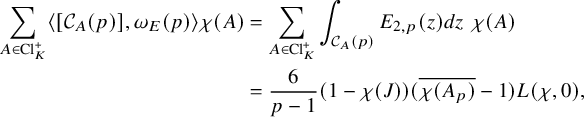 $$ \begin{align}\nonumber \sum_{A\in \mathrm{Cl}_K^+} \langle [\mathcal{C}_{A}(p)],\omega_{E}(p)\rangle \chi(A)&=\sum_{A\in \mathrm{Cl}_K^+} \int_{\mathcal{C}_{A}(p)} E_{2,p}(z)dz\,\, \chi(A)\\ &= \frac{6}{p-1}(1-\chi(J))(\overline{\chi(A_p)}-1)L(\chi,0), \end{align} $$
using that $(p-1)E_{2,p}(z)=pE_{2}^*(pz)-E_{2}^*(z)$
. Note that the above vanishes when
$(p-1)E_{2,p}(z)=pE_{2}^*(pz)-E_{2}^*(z)$
. Note that the above vanishes when $\chi (J)=1$
or
$\chi (J)=1$
or $\chi (A_p)=1$
.
$\chi (A_p)=1$
.
By the functional equation for odd class group L-functions [Reference Duke, Imamoḡlu and TóthDIT18, p. 13] and the fact that class group characters are self-dual (i.e., $\chi \circ c=\overline {\chi }$
where c denotes complex conjugation), we conclude for
$\chi \circ c=\overline {\chi }$
where c denotes complex conjugation), we conclude for $\chi \in \widehat {\mathrm {Cl}_K^+}$
with
$\chi \in \widehat {\mathrm {Cl}_K^+}$
with $\chi (J)=-1$
that
$\chi (J)=-1$
that
 $$ \begin{align} \overline{L(\chi,0)}=L(\overline{\chi},0)=L(\chi\circ c,0)=L(\chi,0)=\pi^{-2} d_K^{1/2} L(\chi,1)>0.\end{align} $$
By standard estimates for L-functions on the critical line for all $\varepsilon>0$
, there is some uniform (but ineffective) constant
$\varepsilon>0$
, there is some uniform (but ineffective) constant $c_\varepsilon>0$
such that
$c_\varepsilon>0$
such that
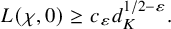 $$ \begin{align} L(\chi,0)\geq c_\varepsilon d_K^{1/2-\varepsilon}.\end{align} $$
Proposition 5.2. Let $H\leq \mathrm {Cl}_K^+$
be a subgroup such that
$H\leq \mathrm {Cl}_K^+$
be a subgroup such that $A_p\notin H$
and
$A_p\notin H$
and $J\notin H$
. Then for each
$J\notin H$
. Then for each $\varepsilon>0$
, there exists a constant
$\varepsilon>0$
, there exists a constant $c_\varepsilon>0$
such that
$c_\varepsilon>0$
such that
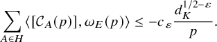 $$ \begin{align} \sum_{A\in H} \langle [\mathcal{C}_{A}(p)], \omega_{E}(p) \rangle \leq -c_\varepsilon \frac{d_K^{1/2-\varepsilon}}{p}. \end{align} $$
Proof. By orthogonality, the Hecke formula (5.7), and equations (5.8) and (5.9), we conclude
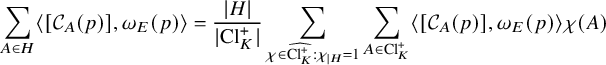 $$ \begin{align} \sum_{A\in H} \langle [\mathcal{C}_{A}(p)], \omega_{E}(p) \rangle&=\frac{|H|}{|\mathrm{Cl}_K^+|}\sum_{\chi\in \widehat{\mathrm{Cl}_K^+}: \chi_{|H}=1}\sum_{A\in \mathrm{Cl}_K^+} \langle [\mathcal{C}_{A}(p)], \omega_{E}(p) \rangle\chi(A)\qquad\qquad\qquad \end{align} $$
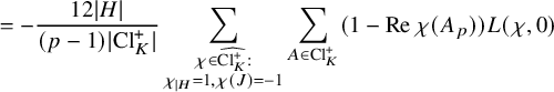 $$ \begin{align} &\qquad\quad\qquad=-\frac{12|H|}{(p-1)|\mathrm{Cl}_K^+|}\sum_{\substack{\chi\in \widehat{\mathrm{Cl}_K^+}:\\ \chi_{|H}=1,\chi(J)=-1}}\sum_{A\in \mathrm{Cl}_K^+} (1-\operatorname{Re} \chi(A_p))L(\chi,0) \end{align} $$
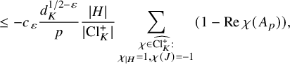 $$ \begin{align} &\qquad\!\!\quad\leq -c_\varepsilon \frac{d_K^{1/2-\varepsilon}}{p}\frac{|H|}{|\mathrm{Cl}_K^+|}\sum_{\substack{\chi\in \widehat{\mathrm{Cl}_K^+}:\\ \chi_{|H}=1,\chi(J)=-1}} (1-\operatorname{Re} \chi(A_p)),\qquad \end{align} $$
where we are using that $(1-\operatorname {Re} \chi (A_p))\geq 0$
. Now we observe that if
$(1-\operatorname {Re} \chi (A_p))\geq 0$
. Now we observe that if $H':=\langle H,J\rangle \leq \mathrm {Cl}_K^+$
denotes the group generated by
$H':=\langle H,J\rangle \leq \mathrm {Cl}_K^+$
denotes the group generated by $H\leq \mathrm {Cl}_K^+$
and
$H\leq \mathrm {Cl}_K^+$
and $J=(\sqrt {d_K})$
, then we can write
$J=(\sqrt {d_K})$
, then we can write
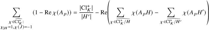 $$ \begin{align} \sum_{\substack{\chi\in \widehat{\mathrm{Cl}_K^+}:\\ \chi_{|H}=1,\chi(J)=-1}} (1-\operatorname{Re} \chi(A_p)) &= \frac{|\mathrm{Cl}_K^+|}{|H'|} -\operatorname{Re} \left( \sum_{\substack{\chi\in \widehat{\mathrm{Cl}_K^+/H}}} \chi(A_p H)-\sum_{\substack{\chi\in \widehat{\mathrm{Cl}_K^+/H'}}}\chi(A_p H') \right) \end{align} $$
 $$ \begin{align} &\,\kern-1.3pt= \begin{cases} \tfrac{|\mathrm{Cl}_K^+|}{2|H|},& A_p\notin H'\\ \frac{|\mathrm{Cl}_K^+|}{|H|},& A_p\in H'\end{cases}.\quad\quad\qquad \end{align} $$
Here, we are using that $J\notin H$
, which implies that
$J\notin H$
, which implies that $|H'|=2|H|$
, and
$|H'|=2|H|$
, and $A_p\notin H$
. Inserting this into the above yields the wanted estimate.
$A_p\notin H$
. Inserting this into the above yields the wanted estimate.
5.2 The cuspidal contribution
In the case of cuspidal Weyl sums, we will use the following formula due to Popa [Reference PopaPop06, Theorem 6.3.1] (see also the first formula in the introduction of [Reference PopaPop06]):
 $$ \begin{align} \left|\sum_{A\in \mathrm{Cl}_K^+} \langle [\mathcal{C}_{A}(p)], \omega_f \rangle \overline{\chi}(A)\right|^2=d_K^{1/2}L(\pi_f\otimes \pi_\chi,1/2), \end{align} $$
where $\pi _f$
denotes the
$\pi _f$
denotes the $\mathrm {GL}_2$
-automorphic representation associated to f,
$\mathrm {GL}_2$
-automorphic representation associated to f, $\pi _\chi $
denotes the
$\pi _\chi $
denotes the $\mathrm {GL}_2$
-automorphic representation associated to
$\mathrm {GL}_2$
-automorphic representation associated to $\chi $
via automorphic induction and
$\chi $
via automorphic induction and $L(\pi _f\otimes \pi _\chi ,1/2)$
denotes the central value of the (finite part of the) Rankin–Selberg L-function of
$L(\pi _f\otimes \pi _\chi ,1/2)$
denotes the central value of the (finite part of the) Rankin–Selberg L-function of $\pi _f$
and
$\pi _f$
and $\pi _\chi $
. This implies
$\pi _\chi $
. This implies
 $$ \begin{align} \sum_{A\in \mathrm{Cl}_K^+} \langle [\mathcal{C}_{A}(p)], \omega_f^{\pm} \rangle \overline{\chi}(A) = \frac{d_K^{1/4}}{2}\left( \epsilon_{f,\chi} |L(\pi_f\otimes \pi_\chi,1/2)|^{1/2}\pm \epsilon_{f,\overline{\chi}} |L(\pi_f\otimes \pi_{\overline{\chi}},1/2)|^{1/2} \right), \end{align} $$
with $|\epsilon _{f,\chi }|=|\epsilon _{f,\overline {\chi }}|=1$
. By the subconvexity bound
$|\epsilon _{f,\chi }|=|\epsilon _{f,\overline {\chi }}|=1$
. By the subconvexity bound
 $$ \begin{align*} L(\pi_f\otimes \pi_{\chi},1/2)\ll_f d_K^{1/2-1/1057}\end{align*} $$
due to Michel [Reference MichelMic04, Theorem 2], we conclude the following bound on the twisted Weyl sums:
 $$ \begin{align}\sum_{A\in \mathrm{Cl}_K^+} \langle [\mathcal{C}_{A}(p)], \omega_f^{\pm} \rangle \overline{\chi}(A)\ll_f d_K^{1/2-1/2114}.\end{align} $$
Combining this with the lower bound for the Eisenstein contribution yields the proof of our main result.
Proof of Theorem 5.1
Let $H\leq \mathrm {Cl}_K^+$
be a subgroup as in the statement. Then by Proposition 5.2, we have for all
$H\leq \mathrm {Cl}_K^+$
be a subgroup as in the statement. Then by Proposition 5.2, we have for all $\varepsilon>0$
that there exists an absolute constant
$\varepsilon>0$
that there exists an absolute constant $c_\varepsilon>0$
such that
$c_\varepsilon>0$
such that
 $$ \begin{align}\left|\sum_{A\in H} \langle [\mathcal{C}_{A}(p)], \omega_{E}(p) \rangle\right|=-\sum_{A\in H} \langle [\mathcal{C}_{A}(p)], \omega_{E}(p) \rangle\geq c_\varepsilon d_K^{1/2-\varepsilon}p^{-1}.\end{align} $$
Now the result follows from (5.6) (with $C=1$
) by dividing through by (5.19) and bounding the cuspidal contribution using (5.18). Here, we are using that the number of narrow class group characters
$C=1$
) by dividing through by (5.19) and bounding the cuspidal contribution using (5.18). Here, we are using that the number of narrow class group characters $\chi $
such that
$\chi $
such that $\chi _{|H}=1$
is exactly
$\chi _{|H}=1$
is exactly $\tfrac {|\mathrm {Cl}_K^+|}{|H|}$
, and the remaining terms in (5.6) do not depend on
$\tfrac {|\mathrm {Cl}_K^+|}{|H|}$
, and the remaining terms in (5.6) do not depend on $d_K$
.
$d_K$
.
6 A homological version of the sup norm problem
In this section, we will deal with the problem of obtaining a version of Theorem 5.1 where the level p is allowed to vary. By (5.6) and (5.17), this requires, first of all, bounds for $L(\pi _f\otimes \pi _{\chi },1/2)$
in terms of both
$L(\pi _f\otimes \pi _{\chi },1/2)$
in terms of both $d_K $
and p which in the case of genus characters has been studied by Petrow and Young [Reference Petrow and YoungPY19]. Secondly, we will need estimates for the cap product pairings
$d_K $
and p which in the case of genus characters has been studied by Petrow and Young [Reference Petrow and YoungPY19]. Secondly, we will need estimates for the cap product pairings $\langle v_f^{\pm }, \omega \rangle $
(with
$\langle v_f^{\pm }, \omega \rangle $
(with $f\in \mathcal {B}_p$
) in terms of p. This can be thought of as an analogue of the sup norm problem from arithmetic quantum chaos (see, for example, [Reference Blomer and HolowinskyBH10]) as we will explain below. We will have to restrict to certain compatible families of
$f\in \mathcal {B}_p$
) in terms of p. This can be thought of as an analogue of the sup norm problem from arithmetic quantum chaos (see, for example, [Reference Blomer and HolowinskyBH10]) as we will explain below. We will have to restrict to certain compatible families of $\omega \in H^1(Y_0(p),\mathbb {R})$
, which in our case will be dual bases of basic bases of level p as in Definition 4.7.
$\omega \in H^1(Y_0(p),\mathbb {R})$
, which in our case will be dual bases of basic bases of level p as in Definition 4.7.
Theorem 6.1. Let p be prime and let ${B}\subset H_1(Y_0(p),\mathbb {Z})$
be a basic basis of level p. Then for
${B}\subset H_1(Y_0(p),\mathbb {Z})$
be a basic basis of level p. Then for $\omega \in B^{\ast }$
(the dual basis of B with respect to (3.4)), we have
$\omega \in B^{\ast }$
(the dual basis of B with respect to (3.4)), we have
 $$ \begin{align}\sum_{\epsilon\in \{\pm\}}\sum_{f\in \mathcal{B}_p} | \langle v_f^{\epsilon}, \omega\rangle|^2 \ll_\varepsilon p^{1+\varepsilon} .\end{align} $$
See Remark 6.2 below for thoughts on the optimal bound that one can expect. Notice that since the newforms $f\in \mathcal {B}_p$
are Hecke normalized, the dual vectors
$f\in \mathcal {B}_p$
are Hecke normalized, the dual vectors $v_f^{\pm }$
are very subtle quantities as they are related to the minimal periods
$v_f^{\pm }$
are very subtle quantities as they are related to the minimal periods $c_f^{\pm }$
of f (characterized when f has rational coefficients by
$c_f^{\pm }$
of f (characterized when f has rational coefficients by $(c_f^{+})^{-1} \operatorname {Re} f(z)dz\in H^1(X_0(p), \mathbb {Z})$
being primitive, and similarly for
$(c_f^{+})^{-1} \operatorname {Re} f(z)dz\in H^1(X_0(p), \mathbb {Z})$
being primitive, and similarly for $c_f^{-}$
). Upper bounding
$c_f^{-}$
). Upper bounding $c_f^{\pm }$
in terms of the level is extremely hard as any polynomial bound implies (a weak form of) the ABC-conjecture (see [Reference GoldfeldGol02]).
$c_f^{\pm }$
in terms of the level is extremely hard as any polynomial bound implies (a weak form of) the ABC-conjecture (see [Reference GoldfeldGol02]).
To put Theorem 6.1 into perspective, it is again useful to compare to the imaginary quadratic analogue of supersingular reduction of CM elliptic curves. Recall that in Section 2 we defined an n-dimensional vector space $H_0(X^{p,\infty },\mathbb {R})$
having a canonical basis
$H_0(X^{p,\infty },\mathbb {R})$
having a canonical basis $e_1,\ldots , e_n$
corresponding to the connected components of the conic curve
$e_1,\ldots , e_n$
corresponding to the connected components of the conic curve $X^{p,\infty }$
as defined in (2.2), which, in turn, can be identified with isomorphism classes of supersingular elliptic curves defined over
$X^{p,\infty }$
as defined in (2.2), which, in turn, can be identified with isomorphism classes of supersingular elliptic curves defined over $\mathbb {F}_{p^2}$
. There is a canonical bilinear form
$\mathbb {F}_{p^2}$
. There is a canonical bilinear form $\langle \cdot , \cdot \rangle _{\mathrm {ss}}$
on
$\langle \cdot , \cdot \rangle _{\mathrm {ss}}$
on $H_0(X^{p,\infty },\mathbb {R})$
given by
$H_0(X^{p,\infty },\mathbb {R})$
given by
 $$ \begin{align}\langle e_i, e_j \rangle_{\mathrm{ss}}:= \delta_{i,j}w_i,\end{align} $$
where $w_i$
is the size of the endomorphism ring of the elliptic curves corresponding to
$w_i$
is the size of the endomorphism ring of the elliptic curves corresponding to $e_i$
. The homology group
$e_i$
. The homology group $H_0(X^{p,\infty },\mathbb {R})$
carries a natural action of the Hecke algebra (of level p) defined via correspondences, and these linear operators are self-adjoint with respect to the bilinear form
$H_0(X^{p,\infty },\mathbb {R})$
carries a natural action of the Hecke algebra (of level p) defined via correspondences, and these linear operators are self-adjoint with respect to the bilinear form $\langle \cdot , \cdot \rangle _{\mathrm {ss}}$
. The homology group
$\langle \cdot , \cdot \rangle _{\mathrm {ss}}$
. The homology group $H_0(X^{p,\infty },\mathbb {R})$
is (by the Jacquet–Langlands correspondence) isomorphic as a Hecke algebra to the space
$H_0(X^{p,\infty },\mathbb {R})$
is (by the Jacquet–Langlands correspondence) isomorphic as a Hecke algebra to the space $\mathcal {M}_2(p)$
of holomorphic modular forms of level p and weight 2. In particular, one can associate to each Hecke eigenform f a unique element
$\mathcal {M}_2(p)$
of holomorphic modular forms of level p and weight 2. In particular, one can associate to each Hecke eigenform f a unique element $e_f\in H_0(X^{p,\infty },\mathbb {R})$
such that
$e_f\in H_0(X^{p,\infty },\mathbb {R})$
such that $\langle e_f, e_f \rangle _{\mathrm {ss}}=1$
and
$\langle e_f, e_f \rangle _{\mathrm {ss}}=1$
and $T_\ell \, e_f=\lambda _f(\ell )e_f$
, where
$T_\ell \, e_f=\lambda _f(\ell )e_f$
, where $\lambda _f(\ell )$
denotes the
$\lambda _f(\ell )$
denotes the $\ell $
-th Hecke eigenvalues of f with
$\ell $
-th Hecke eigenvalues of f with $\ell \neq p$
prime. In this setting, we are interested in upper bounds for the ‘
$\ell \neq p$
prime. In this setting, we are interested in upper bounds for the ‘ $L^r$
-norms’:
$L^r$
-norms’:
 $$ \begin{align*} |\!|e_f|\!|_r:=\left(\sum_{i=1}^n |\langle e_f, e_i \rangle_{\mathrm{ss}}|^r\right)^{1/r}, 1\leq r< \infty,\quad |\!|e_f|\!|_\infty:=\max_{1\leq i\leq n}|\langle e_f, e_i \rangle_{\mathrm{ss}}|. \end{align*} $$
Putting $r=2$
and using Parseval, one obtains
$r=2$
and using Parseval, one obtains $|\!|e_f|\!|_2=1$
which implies the trivial (or convexity) bound
$|\!|e_f|\!|_2=1$
which implies the trivial (or convexity) bound $|\!|e_f|\!|_r\leq 1 $
for all
$|\!|e_f|\!|_r\leq 1 $
for all $r\geq 2$
. In the case
$r\geq 2$
. In the case $r=\infty $
, Blomer and Michel [Reference Blomer and MichelBM11] were the first to go beyond this by proving
$r=\infty $
, Blomer and Michel [Reference Blomer and MichelBM11] were the first to go beyond this by proving $|\!|e_f|\!|_\infty \ll p^{-1/6+\varepsilon }$
. This was recently improved by Khayutin–Nelson–Steiner [Reference Khayutin, Nelson and SteinerKNS22, Corollary 2.3] who obtained
$|\!|e_f|\!|_\infty \ll p^{-1/6+\varepsilon }$
. This was recently improved by Khayutin–Nelson–Steiner [Reference Khayutin, Nelson and SteinerKNS22, Corollary 2.3] who obtained $|\!|e_f|\!|_\infty \ll p^{-1/4+\varepsilon }$
. Liu–Masri–Young [Reference Liu, Masri and YoungLMY15, Proposition 1.12] obtained the
$|\!|e_f|\!|_\infty \ll p^{-1/4+\varepsilon }$
. Liu–Masri–Young [Reference Liu, Masri and YoungLMY15, Proposition 1.12] obtained the $L^4$
-bound
$L^4$
-bound $|\!|e_f|\!|_4\ll p^{-1/8+\varepsilon }$
.
$|\!|e_f|\!|_4\ll p^{-1/8+\varepsilon }$
.
The fact that the Hecke operators are self-adjoint with respect to the bilinear form (6.2) on $H_0(X^{p,\infty },\mathbb {R})$
implies that the dual basis
$H_0(X^{p,\infty },\mathbb {R})$
implies that the dual basis
 $$ \begin{align*} e_1^\ast,\ldots, e_n^\ast\in H_0(X^{p,\infty},\mathbb{R})^\ast \end{align*} $$
of $e_1,\ldots , e_n$
(which we can identify with
$e_1,\ldots , e_n$
(which we can identify with $w_1^{-1}\langle \cdot , e_1\rangle _{\mathrm {ss}},\ldots , w_n^{-1}\langle \cdot , e_n\rangle _{\mathrm {ss}}$
) have the same behavior under the action of the Hecke algebra. This is why in the proof of the level aspect version (2.5) by Liu–Masri–Young one does not need any nontrivial input to bound the factors
$w_1^{-1}\langle \cdot , e_1\rangle _{\mathrm {ss}},\ldots , w_n^{-1}\langle \cdot , e_n\rangle _{\mathrm {ss}}$
) have the same behavior under the action of the Hecke algebra. This is why in the proof of the level aspect version (2.5) by Liu–Masri–Young one does not need any nontrivial input to bound the factors $\langle e_f, e_i\rangle _{\mathrm {ss}}$
appearing when spectrally expanding; one can simply employ the trivial Parseval bound
$\langle e_f, e_i\rangle _{\mathrm {ss}}$
appearing when spectrally expanding; one can simply employ the trivial Parseval bound $\sum _{f\in \mathcal {B}_p} |\langle e_f, e_i\rangle _{\mathrm {ss}}|^2\leq 1$
.This is not necessarily the case for the basic bases
$\sum _{f\in \mathcal {B}_p} |\langle e_f, e_i\rangle _{\mathrm {ss}}|^2\leq 1$
.This is not necessarily the case for the basic bases ${B}\subset H_1(Y_0(p), \mathbb {R})$
in our setting. This means, in particular, that we do not know whether
${B}\subset H_1(Y_0(p), \mathbb {R})$
in our setting. This means, in particular, that we do not know whether
 $$ \begin{align}\langle v , \omega_f^{\pm}\rangle \langle v_f^{\pm}, v^\ast \rangle \end{align} $$
is positive or not for $v\in {B}$
and
$v\in {B}$
and $v^\ast \in B^{\ast }$
such that
$v^\ast \in B^{\ast }$
such that $\langle v, v^\ast \rangle =1$
. This lack of positivity makes it hard to obtain any bound at all.
$\langle v, v^\ast \rangle =1$
. This lack of positivity makes it hard to obtain any bound at all.
6.1 The method of proof
The first natural approach to bounding the left-hand side of (6.1) would be to use a version of the amplified pre-trace formula approach to the sup norm problem in arithmetic quantum chaos (see, for example, [Reference Blomer and HolowinskyBH10]). This is, however, not very effective due to the possible non-positivity of (6.3) (i.e., we are working in a Banach space rather than a Hilbert space). However, it has become apparent from the work of Steiner [Reference SteinerSte20], Khayutin–Steiner [Reference Khayutin and SteinerKS20] and Khayutin–Nelson–Steiner [Reference Khayutin, Nelson and SteinerKNS22] that one in many cases can obtain very strong sup norm bounds by using the theta correspondence. We will employ a version of this argument in our setting. The basic fact is that for $v_0\in H_1(X_0(p),\mathbb {R})$
and
$v_0\in H_1(X_0(p),\mathbb {R})$
and $\omega \in H^1(X_0(p),\mathbb {R})$
,
$\omega \in H^1(X_0(p),\mathbb {R})$
,
 $$ \begin{align}\sum_{n\geq 1} \langle T_n v_0, \omega\rangle e^{2\pi i nz}\end{align} $$
defines a cusp form of level p. This follows easily by the fact that the $\pm 1$
isotypic components of
$\pm 1$
isotypic components of $\iota $
acting on
$\iota $
acting on $H_1(X_0(p), \mathbb {R})$
are isomorphic as Hecke modules to the space of holomorphic cusp forms
$H_1(X_0(p), \mathbb {R})$
are isomorphic as Hecke modules to the space of holomorphic cusp forms $\mathcal {S}_2(p)$
of weight 2 and level p (which is an incarnation of the Eichler–Shimura isomorphism [Reference ShimuraShi94, Section 8.2]). This can be seen as an instance of the theta correspondence (see [Reference Darmon, Harris, Rotger and VenkateshDHRV21, Section 5.3]). We will give a simple proof below of the exact statement that we need. Now the key fact is that if
$\mathcal {S}_2(p)$
of weight 2 and level p (which is an incarnation of the Eichler–Shimura isomorphism [Reference ShimuraShi94, Section 8.2]). This can be seen as an instance of the theta correspondence (see [Reference Darmon, Harris, Rotger and VenkateshDHRV21, Section 5.3]). We will give a simple proof below of the exact statement that we need. Now the key fact is that if $\iota v_0=\pm v_0$
, then the
$\iota v_0=\pm v_0$
, then the $L^2$
-norm of (6.4) is (by spectrally expanding) equal to
$L^2$
-norm of (6.4) is (by spectrally expanding) equal to
 $$ \begin{align*} \sum_{f\in \mathcal{B}_p} |\langle v_0 , \omega_f^{\pm}\rangle|^ 2 |\langle v_f^{\pm}, \omega \rangle| ^2.\end{align*} $$
Note that now we have obtained positivity for free! Thus, we are reduced to, one the one hand, a lower bound for $|\langle v_0 , \omega _f^{\pm }\rangle |^ 2$
which we resolve in Corollary 6.5, and on the other hand, a bound for the
$|\langle v_0 , \omega _f^{\pm }\rangle |^ 2$
which we resolve in Corollary 6.5, and on the other hand, a bound for the $L^2$
-norm of (6.4) which is essentially equal to
$L^2$
-norm of (6.4) which is essentially equal to
 $$ \begin{align}\sum_{1\leq n\leq p} \frac{|\langle T_n v_0, \mathbb{P}_{\mathrm{cusp}}\,\omega\rangle|^2}{n}.\end{align} $$
The above is an analogue of the second moment matrix count that appears in, for example, [Reference Khayutin and SteinerKS20, Section 9]. We will bound (6.5) using geometric coding of geodesics.
Remark 6.2. Let B be a basic basis of level p and let $v\in B$
and
$v\in B$
and $v^\ast \in B^{\ast }$
such that
$v^\ast \in B^{\ast }$
such that $\langle v, v^\ast \rangle =1$
. Then we get by expanding in the Hecke basis
$\langle v, v^\ast \rangle =1$
. Then we get by expanding in the Hecke basis
 $$ \begin{align*} 1= \sum_{f\in \mathcal{B}_p,\pm } \langle v_f^\pm, v^\ast \rangle \langle v, \omega_f^\pm \rangle.\end{align*} $$
As we will see in Corollary 6.5, we have on average that $\langle v, \omega _f^\pm \rangle \asymp 1$
. Thus, if the classes
$\langle v, \omega _f^\pm \rangle \asymp 1$
. Thus, if the classes $v_f^\pm $
are perfectly distributed (relative to B), then we would have
$v_f^\pm $
are perfectly distributed (relative to B), then we would have $\langle v_f^\pm , v^\ast \rangle \asymp 1/p$
. Thus, the strongest sup norm conjecture one can hope for is
$\langle v_f^\pm , v^\ast \rangle \asymp 1/p$
. Thus, the strongest sup norm conjecture one can hope for is
 $$ \begin{align*} \langle v_f^\pm, \omega \rangle \ll_\varepsilon p^{-1+\varepsilon}, \end{align*} $$
for $\omega \in B^{\ast }$
. This might, however, be too much to hope for.
$\omega \in B^{\ast }$
. This might, however, be too much to hope for.
Remark 6.3. The dual sup norm problem corresponds to obtaining bounds for the modular symbols
 $$ \begin{align*} \sup_{v\in B}\, |\langle v, \omega_f \rangle|, \end{align*} $$
for $v\in B$
as
$v\in B$
as $p\rightarrow \infty $
, where
$p\rightarrow \infty $
, where $\omega _f=f(z)dz$
with
$\omega _f=f(z)dz$
with $f\in \mathcal {B}_p$
a holomorphic Hecke eigenform of weight
$f\in \mathcal {B}_p$
a holomorphic Hecke eigenform of weight $2$
and level p. Let
$2$
and level p. Let $v=\{\gamma z,z\}\in H_1(Y_0(p),\mathbb {Z})$
with
$v=\{\gamma z,z\}\in H_1(Y_0(p),\mathbb {Z})$
with $\gamma \in \mathcal {S}(\mathcal {F}_{\mathrm {Zag}}(p))$
, which we may assume is hyperbolic. Picking z on the fixed circle of
$\gamma \in \mathcal {S}(\mathcal {F}_{\mathrm {Zag}}(p))$
, which we may assume is hyperbolic. Picking z on the fixed circle of $\gamma $
and using Hölder’s inequality, we see that
$\gamma $
and using Hölder’s inequality, we see that
 $$ \begin{align*}\left|\langle v, \omega_f \rangle\right| \leq 2\pi \int_{\mathcal{C}_\gamma} |\operatorname{Im} (z)f(z)|\frac{dz}{\operatorname{Im} (z)}\ll_\varepsilon p^{1/4+\varepsilon} , \end{align*} $$
using the sup norm estimate coming from [Reference Khayutin, Nelson and SteinerKNS22, Theorem 1.6]. Here, $\mathcal {C}_\gamma $
denotes the closed geodesic on
$\mathcal {C}_\gamma $
denotes the closed geodesic on $X_0(p)$
associated to
$X_0(p)$
associated to $\gamma $
with hyperbolic length
$\gamma $
with hyperbolic length $\ell (\mathcal {C}_\gamma )\ll \log p$
. Notice that we also have the trivial bound
$\ell (\mathcal {C}_\gamma )\ll \log p$
. Notice that we also have the trivial bound
 $$ \begin{align*} \left( \sum_{f\in \mathcal{B}_p}\left|\langle v, \omega_f \rangle\right|{}^2\right)^{1/2} \leq 2\pi \int_{\mathcal{C}_\gamma} \left(\sum_{f\in \mathcal{B}_p} |\operatorname{Im} (z)f(z)|^2\right)^{1/2}\frac{dz}{\operatorname{Im} (z)}\ll_\varepsilon p^{1/2+\varepsilon} \end{align*} $$
by Minkowski’s integral inequality and the pre-trace formula (thanks to the referee for pointing this out).
6.2 A lower bound for modular symbols
In this section, we will construct the homology class $v_0\in H_1(X_0(p), \mathbb {R})$
mentioned above such that
$v_0\in H_1(X_0(p), \mathbb {R})$
mentioned above such that $\langle v_0, \omega _f^{\pm }\rangle $
is ‘not too small’ in terms of the level. We will be constructing
$\langle v_0, \omega _f^{\pm }\rangle $
is ‘not too small’ in terms of the level. We will be constructing $v_0$
in terms of classes of the shape
$v_0$
in terms of classes of the shape $\{\tfrac {x}{p},\infty \}$
for
$\{\tfrac {x}{p},\infty \}$
for $1\leq x< p$
(using the notation (3.6)). This reduces the problem to a lower bound for the additive twist L-functions of f. One could naively try to calculate the average of all additive twists with
$1\leq x< p$
(using the notation (3.6)). This reduces the problem to a lower bound for the additive twist L-functions of f. One could naively try to calculate the average of all additive twists with $1\leq x<p$
. But this yields very poor results as there is a lot of cancellation in this sum. Instead, we use that the second moment coincides with the second moment of Dirichlet twists of the L-function of f (by the Birch–Stevens formula). By Cauchy–Schwarz, it suffices to calculate the first moment of these L-functions instead. Such a calculation is quite standard using an approximate functional equation. The exact case we need, however, does not seem to have been considered before as we are in the case of joint ramification. For the sake of completeness, we have provided a detailed argument below.
$1\leq x<p$
. But this yields very poor results as there is a lot of cancellation in this sum. Instead, we use that the second moment coincides with the second moment of Dirichlet twists of the L-function of f (by the Birch–Stevens formula). By Cauchy–Schwarz, it suffices to calculate the first moment of these L-functions instead. Such a calculation is quite standard using an approximate functional equation. The exact case we need, however, does not seem to have been considered before as we are in the case of joint ramification. For the sake of completeness, we have provided a detailed argument below.
To be more precise, let $f\in \mathcal {B}_p$
be a Hecke normalized eigenform and let
$f\in \mathcal {B}_p$
be a Hecke normalized eigenform and let $\chi $
be a primitive Dirichlet character modulo q with
$\chi $
be a primitive Dirichlet character modulo q with $p|q$
. Then we define the twisted L-function as the analytic continuation of
$p|q$
. Then we define the twisted L-function as the analytic continuation of
 $$ \begin{align*} L(f,\chi,s):= \sum_{n\geq 1}\frac{\lambda_f(n)\chi(n)}{n^{s+1/2}} \end{align*} $$
(here the Ramanujan conjecture is $|\lambda _f(n)|\leq d(n)n^{1/2}$
). By the Birch–Stevens formula (see, for example, [Reference NordentoftNor21, Proposition 6.1]), we have for a primitive
$|\lambda _f(n)|\leq d(n)n^{1/2}$
). By the Birch–Stevens formula (see, for example, [Reference NordentoftNor21, Proposition 6.1]), we have for a primitive $\chi $
with
$\chi $
with $\chi (-1)=\pm 1$
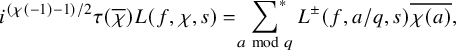 $$ \begin{align} i^{(\chi(-1)-1)/2}\tau(\overline{\chi})L(f,\chi,s)= \sideset{}{^\ast}\sum_{a \ \mathrm {mod}\ q} L^{\pm}(f, a/q,s)\overline{\chi(a)},\end{align} $$
where
 $$ \begin{align*} L^\pm(f, a/q,s):=\frac{L(f, a/q,s)\pm L(f, -a/q,s)}{1+i\pm (1-i)}, \quad L(f, a/q,s):=\sum_{n\geq 1} \frac{\lambda_f(n)e(na/q)}{n^{s+1/2}},\quad \operatorname{Re} s>1 \end{align*} $$
are the additive twist L-series satisfying analytic continuation and the functional equation
 $$ \begin{align*} \gamma_f(s)q^s L(f,a/q,s)= -\gamma_f(1-s)q^{1-s} L(f,-\overline{a}/q,1-s), \end{align*} $$
where $a\overline{a}\equiv 1\ \mathrm{mod}\ q$
and
$a\overline{a}\equiv 1\ \mathrm{mod}\ q$
and $\gamma_f(s)=\Gamma(s+1/2)(2\pi)^{-s}$
(see e.g. Reference NordentoftNor21, Proposition 3.3). This implies the functional equation
$\gamma_f(s)=\Gamma(s+1/2)(2\pi)^{-s}$
(see e.g. Reference NordentoftNor21, Proposition 3.3). This implies the functional equation
 $$ \begin{align}\gamma_f(s)q^{s} L(f,\chi,s)=\varepsilon_\chi \gamma_f(1-s)q^{1-s} L(f,\overline{\chi},1-s),\end{align} $$
where $\varepsilon _\chi = \frac {-\tau (\chi )^2}{q}$
. Note that by inserting the Fourier expansion of f and interchanging sum and integral, we arrive at the identity
$\varepsilon _\chi = \frac {-\tau (\chi )^2}{q}$
. Note that by inserting the Fourier expansion of f and interchanging sum and integral, we arrive at the identity
 $$ \begin{align}\langle \{\tfrac{a}{q},\infty\}, \omega^\pm_f\rangle=-L^\pm(f,\tfrac{a}{q}, 1/2 ).\end{align} $$
Lemma 6.4. Let $f\in \mathcal {B}_p$
and let q be an integer such that
$f\in \mathcal {B}_p$
and let q be an integer such that $p|q$
. Then we have (uniformly in p and f) that
$p|q$
. Then we have (uniformly in p and f) that
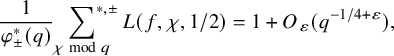 $$ \begin{align*} \frac{1}{\varphi^\ast_\pm(q)}\,\,\,\sideset{}{^{\ast,\pm}}\sum_{\chi \ \mathrm {mod}\ q} L(f,\chi,1/2)=1+O_\varepsilon(q^{-1/4+\varepsilon}),\end{align*} $$
where the sum is restricted to primitive characters $\chi $
modulo q with
$\chi $
modulo q with $\chi (-1)=\pm 1$
, and
$\chi (-1)=\pm 1$
, and $\varphi ^*_\pm (q)$
denotes the total number of such characters.
$\varphi ^*_\pm (q)$
denotes the total number of such characters.
Proof. By the approximate functional equation [Reference Iwaniec and KowalskiIK04, Theorem 5.3] using (6.7), we can write the moment in question as
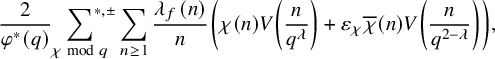 $$ \begin{align} \frac{2}{\varphi^*(q)}\,\,\,\sideset{}{^{\ast,\pm}}\sum_{\chi \ \mathrm {mod}\ q} \sum_{n\geq 1} \frac{\lambda_f(n)}{n}\left(\chi(n) V\left(\frac{n}{q^\lambda}\right)+ \varepsilon_\chi \overline{\chi}(n) V\left(\frac{n}{q^{2-\lambda}}\right)\right), \end{align} $$
for some $0<\lambda <2$
to be chosen and
$0<\lambda <2$
to be chosen and $V: \mathbb {R}_{>0}\rightarrow \mathbb {R}$
a smooth, rapidly decaying function satisfying
$V: \mathbb {R}_{>0}\rightarrow \mathbb {R}$
a smooth, rapidly decaying function satisfying $V(y)=1+O(y^{1/3})$
as
$V(y)=1+O(y^{1/3})$
as $y\rightarrow 0$
(see [Reference Iwaniec and KowalskiIK04, Proposition 5.4]). Now by a simple application of Möbius inversion, we get that for
$y\rightarrow 0$
(see [Reference Iwaniec and KowalskiIK04, Proposition 5.4]). Now by a simple application of Möbius inversion, we get that for $(n,q)=1$
,
$(n,q)=1$
,
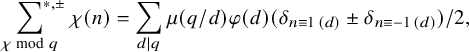 $$ \begin{align} \sideset{}{^{\ast,\pm}}\sum_{\chi \ \mathrm {mod}\ q} \chi(n) &=\sum_{d|q} \mu(q/d)\varphi(d)(\delta_{n\equiv 1 \, (d)}\pm \delta_{n\equiv -1 \, (d)})/2 , \end{align} $$
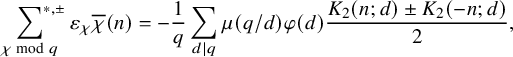 $$ \begin{align} \sideset{}{^{\ast,\pm}}\sum_{\chi \ \mathrm {mod}\ q} \varepsilon_\chi \overline{\chi}(n) &=-\frac{1}{q} \sum_{d|q} \mu(q/d)\varphi(d)\frac{K_2(n;d)\pm K_2(-n;d)}{2}, \end{align} $$
where $K_2(n;d)= \sum _{xy\equiv n\, (d)} e((x+y)/d)$
denotes the usual
$K_2(n;d)= \sum _{xy\equiv n\, (d)} e((x+y)/d)$
denotes the usual $2$
-dimensional Kloosterman sum. By Weil’s bound and standard estimates, we conclude that for
$2$
-dimensional Kloosterman sum. By Weil’s bound and standard estimates, we conclude that for $(n,q)=1$
,
$(n,q)=1$
,
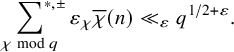 $$ \begin{align} \sideset{}{^{\ast,\pm}}\sum_{\chi \ \mathrm {mod}\ q} \varepsilon_\chi \overline{\chi}(n) \ll_\varepsilon q^{1/2+\varepsilon}. \end{align} $$
Now for the primary part of the sum (6.9) we obtain using the analytic properties of V mentioned above as well as (6.10), we get
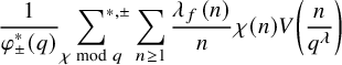 $$ \begin{align} &\frac{1}{\varphi^*_\pm(q)}\,\,\,\sideset{}{^{\ast,\pm}}\sum_{\chi \ \mathrm {mod}\ q} \sum_{n\geq 1} \frac{\lambda_f(n)}{n} \chi(n) V\left(\frac{n}{q^\lambda}\right) \quad\qquad\qquad\end{align} $$
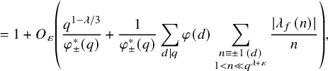 $$ \begin{align} &\quad\qquad=1+O_{\varepsilon}\left(\frac{q^{1-\lambda/3}}{\varphi^*_\pm(q)}+\frac{1}{\varphi^*_\pm(q)}\sum_{d|q} \varphi(d) \sum_{\substack{n\equiv \pm 1\, (d)\\ 1<n\ll q^{\lambda+\varepsilon}}} \frac{|\lambda_f(n)|}{n} \right), \end{align} $$
with the main term corresponding to $n=1$
. Now using the Ramanujan bound
$n=1$
. Now using the Ramanujan bound $|\lambda _f(n)|\leq d(n)n^{1/2}\ll _\varepsilon n^{1/2+\varepsilon }$
, we get
$|\lambda _f(n)|\leq d(n)n^{1/2}\ll _\varepsilon n^{1/2+\varepsilon }$
, we get
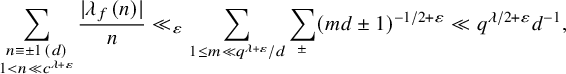 $$ \begin{align} \sum_{\substack{n\equiv \pm 1\, (d)\\ 1<n\ll c^{\lambda+\varepsilon}}} \frac{|\lambda_f(n)|}{n}\ll_\varepsilon \sum_{ 1\leq m \ll q^{\lambda+\varepsilon}/d}\sum_\pm (md\pm 1)^{-1/2+\varepsilon}\ll q^{\lambda/2+\varepsilon}d^{-1}, \end{align} $$
which bounds the error-term in (6.13) by $O_\varepsilon ((q^{1-\lambda /3}+q^{\lambda /2+\varepsilon })/\varphi ^\ast (q))$
. Similarly, by using (6.11), we can bound the dual sum by
$O_\varepsilon ((q^{1-\lambda /3}+q^{\lambda /2+\varepsilon })/\varphi ^\ast (q))$
. Similarly, by using (6.11), we can bound the dual sum by $O_\varepsilon (q^{3/2-\lambda /2+\varepsilon }/\varphi ^\ast _\pm (q))$
. Choosing
$O_\varepsilon (q^{3/2-\lambda /2+\varepsilon }/\varphi ^\ast _\pm (q))$
. Choosing $\lambda =3/2$
and recalling that
$\lambda =3/2$
and recalling that $\varphi ^\ast _\pm (q)\gg _\varepsilon q^{1-\varepsilon }$
, we get the wanted asymptotic formula.
$\varphi ^\ast _\pm (q)\gg _\varepsilon q^{1-\varepsilon }$
, we get the wanted asymptotic formula.
Corollary 6.5. There exists an absolute constant $c_0>0$
such that for any prime p,
$c_0>0$
such that for any prime p, $f\in \mathcal {B}_p$
and
$f\in \mathcal {B}_p$
and $\epsilon \in \{\pm \}$
, we have
$\epsilon \in \{\pm \}$
, we have
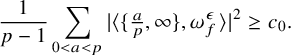 $$ \begin{align} \frac{1}{p-1}\sum_{0<a <p} |\langle\{\tfrac{a}{p},\infty\},\omega_f^{\epsilon} \rangle|^2\geq c_0. \end{align} $$
Proof. First of all, recall that the following matrices generate $\Gamma _0(p)$
:
$\Gamma _0(p)$
:
where $0<a^\ast <p$
are such that
$0<a^\ast <p$
are such that $a\overline {a}\equiv -1 \ \mathrm {mod}\ p$
(as is proved in Section 4.2). Since
$a\overline {a}\equiv -1 \ \mathrm {mod}\ p$
(as is proved in Section 4.2). Since $\omega _f^{\pm }$
are nonzero cohomology classes vanishing on parabolic elements, we conclude that the left-hand side of (6.16) is always nonzero.
$\omega _f^{\pm }$
are nonzero cohomology classes vanishing on parabolic elements, we conclude that the left-hand side of (6.16) is always nonzero.
We now define the Fourier transform of
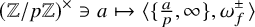 $$ \begin{align*} (\mathbb{Z}/p\mathbb{Z})^\times \ni a\mapsto \langle\{\tfrac{a}{p},\infty\},\omega_f^{\pm} \rangle \end{align*} $$
as follows for a Dirichlet character $\chi \ \mathrm {mod}\ p$
:
$\chi \ \mathrm {mod}\ p$
:
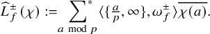 $$ \begin{align*} \widehat{L}_f^{\pm}(\chi):= \sideset{}{^\ast}\sum_{a \ \mathrm {mod}\ p} \langle\{\tfrac{a}{p},\infty\},\omega_f^{\pm} \rangle \overline{\chi(a)}.\end{align*} $$
For $\chi $
primitive with
$\chi $
primitive with $\chi (-1)=\pm 1$
, we have by the equality (6.8) and the Birch–Stevens formula (6.6) that
$\chi (-1)=\pm 1$
, we have by the equality (6.8) and the Birch–Stevens formula (6.6) that
 $$ \begin{align*} \widehat{L}_f^{\pm}(\chi)= -i^{(\chi(-1)-1)/2}\tau(\overline{\chi})L(f,\chi,1/2). \end{align*} $$
Now by Parseval, we have
 $$ \begin{align*} \sum_{0<a <p} |\langle\{\tfrac{a}{p},\infty\},\omega_f^{\pm} \rangle|^2=\frac{1}{p-1}\sum_{\chi \ \mathrm {mod}\ p} |\widehat{L}_f^{\pm}(\chi)|^2 \geq \frac{p}{p-1}\,\,\,\sideset{}{^{\ast,\pm}}\sum_{\chi \ \mathrm {mod}\ p} |L(f,\chi,1/2)|^2. \end{align*} $$
Using the previous lemma, we conclude by Cauchy–Schwarz that
 $$ \begin{align*} \frac{1}{\varphi^\ast_\pm(p)}\,\,\,\sideset{}{^{\ast,\pm}}\sum_{\chi \ \mathrm {mod}\ p} |L(f,\chi,1/2)|^2\geq \left( \frac{1}{\varphi^\ast_\pm(p)}\,\,\, \sideset{}{^{\ast,\pm}}\sum_{\chi \ \mathrm {mod}\ p} L(f,\chi,1/2)\right)^2\geq 1/2, \end{align*} $$
for p large enough. This yields the wanted lower bound since $\varphi _\pm ^\ast (p)\asymp p-1$
.
$\varphi _\pm ^\ast (p)\asymp p-1$
.
Remark 6.6. Using a subconvexity bound for $L(f\otimes \chi , 1/2)$
as in [Reference Michel and VenkateshMV10], the above implies that there is some constant
$L(f\otimes \chi , 1/2)$
as in [Reference Michel and VenkateshMV10], the above implies that there is some constant $\delta>0$
such that
$\delta>0$
such that $L(f\otimes \chi , 1/2)$
is nonvanishing for at least
$L(f\otimes \chi , 1/2)$
is nonvanishing for at least $\gg p^\delta $
of both odd and even characters. This improves on Merel [Reference MerelMer09, Corollaire 2], who has shown using modular symbol techniques that for
$\gg p^\delta $
of both odd and even characters. This improves on Merel [Reference MerelMer09, Corollaire 2], who has shown using modular symbol techniques that for $f\in \mathcal {B}_p$
, there exists at least one odd and one even character
$f\in \mathcal {B}_p$
, there exists at least one odd and one even character $\chi $
of conductor p such that
$\chi $
of conductor p such that $L(f\otimes \chi , 1/2)\neq 0$
. One can probably get much better results using mollification.
$L(f\otimes \chi , 1/2)\neq 0$
. One can probably get much better results using mollification.
6.3 Reduction to a counting problem
We will now use the theta correspondence in a simple form to reduce the sup norm problem to a certain counting problem.
Lemma 6.7. Let $\omega \in H^1(X_0(p),\mathbb {R})$
be a cuspidal cohomology class. Then we have
$\omega \in H^1(X_0(p),\mathbb {R})$
be a cuspidal cohomology class. Then we have
 $$ \begin{align*} \sum_{\epsilon\in \{\pm \}}\sum_{f\in \mathcal{B}_p} | \langle v_f^{\epsilon}, \omega\rangle|^2 \ll_\varepsilon p^{-1+\varepsilon}\sum_{n\geq 1} \frac{\frac{1}{p}\sum_{0< x<p}(|\langle T_n \{\tfrac{x}{p}, \infty\}, \omega \rangle|^2+|\langle T_n \{\tfrac{1}{x}, 0\}, \omega \rangle|^2)}{n} e^{-8 n/p} \end{align*} $$
uniformly in p, where $\langle \cdot , \cdot \rangle $
denotes the cap product pairing (3.4) between homology and cohomology and
$\langle \cdot , \cdot \rangle $
denotes the cap product pairing (3.4) between homology and cohomology and $T_n$
denotes the n-th Hecke operator.
$T_n$
denotes the n-th Hecke operator.
Proof. For $0<x<p$
and
$0<x<p$
and ${\boldsymbol {\epsilon }}=(\epsilon _1,\epsilon _2)$
with
${\boldsymbol {\epsilon }}=(\epsilon _1,\epsilon _2)$
with $\epsilon _i\in \{\pm 1\}$
, we consider the following class in the compactly supported homology
$\epsilon _i\in \{\pm 1\}$
, we consider the following class in the compactly supported homology
 $$ \begin{align} &v_x^{\boldsymbol{\epsilon}}:=(1+\epsilon_1 \iota)(1+\epsilon_2 W_p)\{\tfrac{x}{p} , \infty \}\qquad\qquad\qquad\qquad\quad \end{align} $$
 $$ \begin{align} &\quad \qquad\qquad\qquad\qquad= \{\tfrac{x}{p} , \infty \}+\epsilon_1 \{-\tfrac{x}{p} , \infty \} +\epsilon_2\{-\tfrac{1}{x},0\}+\epsilon_1\epsilon_2 \{\tfrac{1}{x},0\}\in H_1(X_0(p),\mathbb{Z}). \end{align} $$
By construction, $v_x^{\boldsymbol {\epsilon }}$
is contained in the
$v_x^{\boldsymbol {\epsilon }}$
is contained in the $\epsilon _1$
eigenspace of the involution
$\epsilon _1$
eigenspace of the involution $\iota $
as in (3.14), and in the
$\iota $
as in (3.14), and in the $\epsilon _2$
eigenspace of the Fricke involution
$\epsilon _2$
eigenspace of the Fricke involution $W_p$
as in (3.13). Associated to
$W_p$
as in (3.13). Associated to $0<x<p$
,
$0<x<p$
, ${\boldsymbol {\epsilon }}\in \{(\pm 1,\pm 1)\}$
and
${\boldsymbol {\epsilon }}\in \{(\pm 1,\pm 1)\}$
and $\omega \in H^1(X_0(p),\mathbb {R})$
(suppressed in the notation), we define
$\omega \in H^1(X_0(p),\mathbb {R})$
(suppressed in the notation), we define $g:\mathbb {H}\rightarrow \mathbb {C}$
by
$g:\mathbb {H}\rightarrow \mathbb {C}$
by
 $$ \begin{align} g(z):=\sum_{n\geq 1} \langle T_n v_x^{\boldsymbol{\epsilon}}, \omega \rangle e^{2\pi i nz}.\end{align} $$
By expanding in the Hecke basis of cohomology, we obtain
 $$ \begin{align*} \langle T_n v_x^{\boldsymbol{\epsilon}}, \omega \rangle =\sum_{\substack{f\in \mathcal{B}_p:\\ W_p f=\epsilon_2 f}} \lambda_f(n) \langle v_x^{\boldsymbol{\epsilon}}, \omega_f^{\epsilon_1}\rangle \langle v_f^{\epsilon_1}, \omega\rangle. \end{align*} $$
By newform theory, we know that for $f\in \mathcal {B}_p$
, we have
$f\in \mathcal {B}_p$
, we have $\lambda _f(n)=a_f(n)$
, where
$\lambda _f(n)=a_f(n)$
, where $a_f(n)$
denotes the Fourier coefficients (at
$a_f(n)$
denotes the Fourier coefficients (at $\infty $
) of f. Thus, we conclude that
$\infty $
) of f. Thus, we conclude that
 $$ \begin{align*} g(z)= \sum_{\substack{f\in \mathcal{B}_p:\\ W_p f=\epsilon_2 f}} \langle v_x^{\boldsymbol{\epsilon}}, \omega_f^{\epsilon_1}\rangle \langle v_f^{\epsilon_1}, \omega\rangle f(z), \end{align*} $$
and, in particular, $g\in S_2(p)$
is a holomorphic cusp form of weight
$g\in S_2(p)$
is a holomorphic cusp form of weight $2$
for
$2$
for $\Gamma _0(p)$
contained in the
$\Gamma _0(p)$
contained in the $\epsilon _2$
eigenspace of
$\epsilon _2$
eigenspace of $W_p$
. This can be seen as an instance of the theta correspondence as explained above. By orthogonality of Hecke eigenforms, this implies the key identity
$W_p$
. This can be seen as an instance of the theta correspondence as explained above. By orthogonality of Hecke eigenforms, this implies the key identity
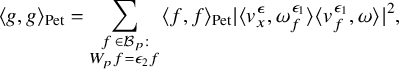 $$ \begin{align} \langle g, g \rangle_{\mathrm{Pet}} = \sum_{\substack{f\in \mathcal{B}_p:\\ W_p f=\epsilon_2 f}} \langle f, f \rangle_{\mathrm{Pet}} |\langle v_x^{{\boldsymbol{\epsilon}}}, \omega_f^{\epsilon_1}\rangle \langle v_f^{\epsilon_1}, \omega\rangle|^2 , \end{align} $$
where $\langle f, g \rangle _{\mathrm {Pet}}= \int _{Y_0(p)} f(z)\overline {g(z)} dxdy$
denotes the Petersson inner-product on
$\langle f, g \rangle _{\mathrm {Pet}}= \int _{Y_0(p)} f(z)\overline {g(z)} dxdy$
denotes the Petersson inner-product on $\mathcal {S}_2(p)$
. Recall from (4.3) that the subgroup
$\mathcal {S}_2(p)$
. Recall from (4.3) that the subgroup
 $$ \begin{align*} \Gamma_0^\ast(p):=\langle W_{p}, \Gamma_0(p)\rangle\subset \mathrm{PSL}_2(\mathbb{R}) \end{align*} $$
has $\Gamma _0(p)$
as an index two subgroup and has a fundamental domain contained in
$\Gamma _0(p)$
as an index two subgroup and has a fundamental domain contained in
 $$ \begin{align*} \{z\in \mathbb{H}: |\operatorname{Re} z| \leq 1/2, \operatorname{Im} z \geq \sqrt{3}/(2p) \}.\end{align*} $$
By unfolding and using that $|g|^2$
is invariant under the Fricke involution
$|g|^2$
is invariant under the Fricke involution $W_p$
, by construction we arrive at the following bound:
$W_p$
, by construction we arrive at the following bound:
 $$ \begin{align}\nonumber\sum_{\substack{f\in \mathcal{B}_p:\\ W_p f=\epsilon_2 f}} \langle f, f \rangle_{\mathrm{Pet}}|\langle v_x^{{\boldsymbol{\epsilon}}}, \omega_f^{\epsilon_1}\rangle \langle v_f^{\epsilon_1}, \omega\rangle|^2=2\int_{\Gamma_0^\ast(p)\backslash \mathbb{H}} |g(z)|^2 dxdy &\ll \int_{\sqrt{3}/(2p)}^\infty \int_{-1/2}^{1/2} |g(z)|^2 dxdy\\ \nonumber&\ll \sum_{n\geq 1} |\langle T_n v_x^{{\boldsymbol{\epsilon}}}, \omega \rangle|^2 \int_{\sqrt{3}/(2p)}^\infty e^{-4\pi n y} dy\\ &\ll \sum_{n\geq 1} \frac{|\langle T_n v_x^{{\boldsymbol{\epsilon}}}, \omega \rangle|^2}{n} e^{-2 \sqrt{3}\pi n/p}. \end{align} $$
Notice that for $f\in \mathcal {B}_p$
with
$f\in \mathcal {B}_p$
with $W_p f=\epsilon _2 f$
, we have by self-adjointness of
$W_p f=\epsilon _2 f$
, we have by self-adjointness of $\iota $
and
$\iota $
and $W_p$
with respect to the cap product pairing that
$W_p$
with respect to the cap product pairing that
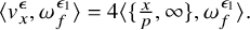 $$ \begin{align*} \langle v_x^{{\boldsymbol{\epsilon}}}, \omega_f^{\epsilon_1}\rangle=4 \langle \{\tfrac{x}{p},\infty\}, \omega_f^{\epsilon_1}\rangle.\end{align*} $$
Now we sum over $0<x<p$
,
$0<x<p$
, $\boldsymbol {\epsilon }\in \{(\pm 1,\pm 1)\}$
and apply Corollary 6.5 to the left-hand side of (6.21). Finally, by expressing the Petersson inner product in terms of a special value of an adjoint L-function (see, for example, [Reference Petridis and RisagerPR18, (8.6)]) and using the lower bounds of Hoffstein–Lockhart [Reference Hoffstein and LockhartHL94], we arrive at
$\boldsymbol {\epsilon }\in \{(\pm 1,\pm 1)\}$
and apply Corollary 6.5 to the left-hand side of (6.21). Finally, by expressing the Petersson inner product in terms of a special value of an adjoint L-function (see, for example, [Reference Petridis and RisagerPR18, (8.6)]) and using the lower bounds of Hoffstein–Lockhart [Reference Hoffstein and LockhartHL94], we arrive at
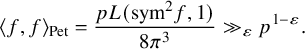 $$ \begin{align*} \langle f, f \rangle_{\mathrm{Pet}}=\frac{pL(\mathrm{sym}^2 f, 1)}{8\pi^3}\gg_\varepsilon p^{1-\varepsilon}.\end{align*} $$
Finally, we have by linearity of $T_n$
that
$T_n$
that
 $$ \begin{align*}|\langle T_n v_x^{{\boldsymbol{\epsilon}}}, \omega \rangle|^2 \ll |\langle T_n \{\tfrac{x}{p} , \infty \}, \omega \rangle|^2+|\langle T_n \{-\tfrac{x}{p} , \infty \}, \omega \rangle|^2+|\langle T_n \{\tfrac{1}{x} , \infty \}, \omega \rangle|^2+|\langle T_n \{-\tfrac{1}{x} , \infty \}, \omega \rangle|^2, \end{align*} $$
from which we conclude the wanted inequality since $2 \sqrt {3}\pi>8$
.
$2 \sqrt {3}\pi>8$
.
6.4 The counting argument
By Lemma 6.7, we are reduced to a certain second moment count. We think of this as an analogue of the matrix counts that show up in most approaches to the (arithmetic) sup norm problem (see, for example, [Reference TemplierTem15]). Recall the Ramanujan bound $|\lambda _f(n)|\leq n^{1/2}d(n)$
for Hecke eigenforms
$|\lambda _f(n)|\leq n^{1/2}d(n)$
for Hecke eigenforms $f\in \mathcal {B}_p$
. This implies for any class
$f\in \mathcal {B}_p$
. This implies for any class $v\in H_1(X_0(p),\mathbb {R})$
and
$v\in H_1(X_0(p),\mathbb {R})$
and $\omega \in H^1(X_0(p),\mathbb {R})$
, we have
$\omega \in H^1(X_0(p),\mathbb {R})$
, we have
 $$ \begin{align*} \langle T_n v, \omega \rangle\ll_{v,\omega} n^{1/2} d(n),\quad \text{as }n\rightarrow \infty. \end{align*} $$
This is, however, not useful as for us the main point is exactly the dependence on v and $\omega $
. Our approach is to use the explicit description of the Hecke operators and then lift the counting from
$\omega $
. Our approach is to use the explicit description of the Hecke operators and then lift the counting from $\Gamma _0(p)^{\mathrm {ab}}$
to
$\Gamma _0(p)^{\mathrm {ab}}$
to $\Gamma _0(p)$
. As a first step, we use geometric coding as in Proposition 4.1 to obtain the following.
$\Gamma _0(p)$
. As a first step, we use geometric coding as in Proposition 4.1 to obtain the following.
Lemma 6.8. Let $\omega \in H^1(X_0(p),\mathbb {R})$
be a cuspidal cohomology class and
$\omega \in H^1(X_0(p),\mathbb {R})$
be a cuspidal cohomology class and
![]() with
with $c> 0$
. Then we have
$c> 0$
. Then we have
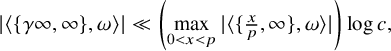 $$ \begin{align} | \langle \{\gamma \infty, \infty \}, \omega \rangle| \ll \left(\max_{0<x<p} |\langle \{\tfrac{x}{p} ,\infty\}, \omega\rangle|\right)\log c,\end{align} $$
uniformly in p.
Proof. Observe that $\{\gamma \infty , \infty \}$
only depends on
$\{\gamma \infty , \infty \}$
only depends on $a/c \ \mathrm {mod}\ 1$
. This means that without changing the homology class, we may assume that
$a/c \ \mathrm {mod}\ 1$
. This means that without changing the homology class, we may assume that $a,d$
are integers satisfying
$a,d$
are integers satisfying $2c\leq |a+d|\leq 4 c $
as well as
$2c\leq |a+d|\leq 4 c $
as well as $-c<a-d<c$
. This implies that all entries of
$-c<a-d<c$
. This implies that all entries of $\gamma $
are
$\gamma $
are $O( c )$
, and that the half circle
$O( c )$
, and that the half circle $S_\gamma $
fixed by
$S_\gamma $
fixed by $\gamma $
intersects the standard fundamental domain
$\gamma $
intersects the standard fundamental domain $\mathcal {F}_{\mathrm {std}}$
for
$\mathcal {F}_{\mathrm {std}}$
for $\mathrm {PSL}_2(\mathbb {Z})$
. Recall Zagier’s fundamental polygon
$\mathrm {PSL}_2(\mathbb {Z})$
. Recall Zagier’s fundamental polygon $\mathcal {F}_{\mathrm {Zag}}'(p)$
for
$\mathcal {F}_{\mathrm {Zag}}'(p)$
for $\Gamma _0(p)$
defined in Section 4.2 which consists of
$\Gamma _0(p)$
defined in Section 4.2 which consists of $\mathrm {PSL}_2(\mathbb {Z})$
-translates of
$\mathrm {PSL}_2(\mathbb {Z})$
-translates of $\mathcal {F}_{\mathrm {std}}$
, as well as the fundamental polygon
$\mathcal {F}_{\mathrm {std}}$
, as well as the fundamental polygon $\mathcal {F}_{\mathrm {Zag}}(p):=W_{p} \mathcal {F}_{\mathrm {Zag}}'(p)$
. This latter polygon has the advantage that all entries of the associated side pairing transformations are of size
$\mathcal {F}_{\mathrm {Zag}}(p):=W_{p} \mathcal {F}_{\mathrm {Zag}}'(p)$
. This latter polygon has the advantage that all entries of the associated side pairing transformations are of size $\leq p$
, whereas for
$\leq p$
, whereas for $\mathcal {F}_{\mathrm {Zag}}'(p)$
, the lower left entry can be of magnitude
$\mathcal {F}_{\mathrm {Zag}}'(p)$
, the lower left entry can be of magnitude $ p^2$
. Notice also that the assumptions on
$ p^2$
. Notice also that the assumptions on $\gamma $
above ensure that the half circle
$\gamma $
above ensure that the half circle $S_\gamma $
fixed by
$S_\gamma $
fixed by $\gamma $
intersects the Siegel domain
$\gamma $
intersects the Siegel domain $\{z\in \mathbb {H}: |\operatorname {Re} z|\leq 1/2, \operatorname {Im} z\geq 1\}$
which is contained in
$\{z\in \mathbb {H}: |\operatorname {Re} z|\leq 1/2, \operatorname {Im} z\geq 1\}$
which is contained in $\mathcal {F}_{\mathrm {Zag}}(p)$
.
$\mathcal {F}_{\mathrm {Zag}}(p)$
.
We now consider the geometric coding of $\gamma $
with respect to
$\gamma $
with respect to $ \mathcal {F}_{\mathrm {Zag}}(p)$
as in Corollary 4.2. This yields an expression
$ \mathcal {F}_{\mathrm {Zag}}(p)$
as in Corollary 4.2. This yields an expression
 $$ \begin{align*} \gamma= \sigma_1\cdots \sigma_{N}, \end{align*} $$
where $\sigma _i\in \mathcal {S}(\mathcal {F}_{\mathrm {Zag}}(p))$
are side pairing transformations. When considering the class
$\sigma _i\in \mathcal {S}(\mathcal {F}_{\mathrm {Zag}}(p))$
are side pairing transformations. When considering the class $\{\gamma \infty , \infty \}\in H_1(X_0(p), \mathbb {Z})$
in the compact homology, we can ignore the parabolic elements among the
$\{\gamma \infty , \infty \}\in H_1(X_0(p), \mathbb {Z})$
in the compact homology, we can ignore the parabolic elements among the $\sigma _i$
’s. More precisely, if
$\sigma _i$
’s. More precisely, if $\sigma ^{\prime }_1,\ldots , \sigma ^{\prime }_\ell $
is the subsequence of
$\sigma ^{\prime }_1,\ldots , \sigma ^{\prime }_\ell $
is the subsequence of $\sigma _1,\ldots ,\sigma _{N}$
consisting of non-parabolic elements, then we have
$\sigma _1,\ldots ,\sigma _{N}$
consisting of non-parabolic elements, then we have
 $$ \begin{align*} \{\gamma \infty, \infty \} =\sum_{i=1}^\ell \{ \sigma^{\prime}_i\infty , \infty \}\in H_1(X_0(p), \mathbb{Z}). \end{align*} $$
Now $\ell $
is exactly the number of intersections between the geodesic from w to
$\ell $
is exactly the number of intersections between the geodesic from w to $\gamma w$
(for any
$\gamma w$
(for any $w\in \mathcal {F}_{\mathrm {Zag}}(p)\cap S_\gamma $
) and
$w\in \mathcal {F}_{\mathrm {Zag}}(p)\cap S_\gamma $
) and $\Gamma _0(p)$
-translates of the sides of
$\Gamma _0(p)$
-translates of the sides of $\mathcal {F}_{\mathrm {Zag}}(p)$
being paired by non-parabolic elements. This is equal to the number of intersections between the geodesic from w to
$\mathcal {F}_{\mathrm {Zag}}(p)$
being paired by non-parabolic elements. This is equal to the number of intersections between the geodesic from w to $\gamma ' w$
(where
$\gamma ' w$
(where $\gamma '=W_{p}\gamma W_{p}^{-1}$
and
$\gamma '=W_{p}\gamma W_{p}^{-1}$
and $w\in \mathcal {F}_{\mathrm {Zag}}'(p)\cap S_{\gamma '}$
) and
$w\in \mathcal {F}_{\mathrm {Zag}}'(p)\cap S_{\gamma '}$
) and $\Gamma _0(p)$
-translates of the non-parabolic sides of
$\Gamma _0(p)$
-translates of the non-parabolic sides of $\mathcal {F}_{\mathrm {Zag}}'(p)$
(this follows by conjugating everything which preserves parabolicity). Recall that for
$\mathcal {F}_{\mathrm {Zag}}'(p)$
(this follows by conjugating everything which preserves parabolicity). Recall that for $\mathcal {F}_{\mathrm {Zag}}'(p)$
, all sides containing a cusp are paired by parabolic elements. Since
$\mathcal {F}_{\mathrm {Zag}}'(p)$
, all sides containing a cusp are paired by parabolic elements. Since $\mathcal {F}_{\mathrm {Zag}}'(p)$
consists of
$\mathcal {F}_{\mathrm {Zag}}'(p)$
consists of $\mathrm {PSL}_2(\mathbb {Z})$
-translates of
$\mathrm {PSL}_2(\mathbb {Z})$
-translates of $\mathcal {F}_{\mathrm {std}}$
, we can bound
$\mathcal {F}_{\mathrm {std}}$
, we can bound $\ell $
by the number of intersections between the geodesic from w to
$\ell $
by the number of intersections between the geodesic from w to $\gamma ' w$
(for
$\gamma ' w$
(for $w\in \mathcal {F}_{\mathrm {std}}\cap S_{\gamma '}$
) and
$w\in \mathcal {F}_{\mathrm {std}}\cap S_{\gamma '}$
) and $\mathrm {PSL}_2(\mathbb {Z})$
-translates of the non-parabolic side of
$\mathrm {PSL}_2(\mathbb {Z})$
-translates of the non-parabolic side of $\mathcal {F}_{\mathrm {std}}$
– that is, the arc
$\mathcal {F}_{\mathrm {std}}$
– that is, the arc
 $$ \begin{align*} \{z\in \mathbb{H}: |z|=1, -1/2<\operatorname{Re} z< 1/2\}. \end{align*} $$
It now follows from a result of Eichler [Reference EichlerEic65, Satz 1] that
 $$ \begin{align*} \ell \ll \log ((a')^2+(b')^2+(c')^2+(d')^2) \ll \log c , \end{align*} $$
where $a',b',c',d'$
are the entries of
$a',b',c',d'$
are the entries of $\gamma '$
, which by the assumptions on the entries of
$\gamma '$
, which by the assumptions on the entries of $\gamma $
are all
$\gamma $
are all $O( p c)= O(c ^2)$
. By definition of
$O( p c)= O(c ^2)$
. By definition of $\mathcal {F}_{\mathrm {Zag}}(p)$
, we have for all
$\mathcal {F}_{\mathrm {Zag}}(p)$
, we have for all $1\leq i\leq \ell $
that
$1\leq i\leq \ell $
that $\sigma ^{\prime }_i\infty $
is of the form
$\sigma ^{\prime }_i\infty $
is of the form $\tfrac {x}{p}$
with
$\tfrac {x}{p}$
with $0<x<p$
. Thus, we conclude
$0<x<p$
. Thus, we conclude
 $$ \begin{align*} |\langle \{\gamma \infty, \infty \},\omega \rangle| \ll \ell \left(\max_{0<x<p} |\langle \{\tfrac{x}{p} ,\infty\}, \omega\rangle|\right)\ll \log c \left(\max_{0<x<p}|\langle \{\tfrac{x}{p} ,\infty\}, \omega\rangle|\right), \end{align*} $$
as wanted.
This implies the following result for basic bases. Recall the definition of the cuspidal projection operator $\mathbb {P}_{\mathrm {cusp}}$
in (3.23).
$\mathbb {P}_{\mathrm {cusp}}$
in (3.23).
Corollary 6.9. Let ${B}$
be a basic basis of level p. Then for
${B}$
be a basic basis of level p. Then for
![]() with
with $c>0$
and
$c>0$
and $\omega \in B^{\ast }$
, we have
$\omega \in B^{\ast }$
, we have
 $$ \begin{align*} |\langle \{\gamma \infty,\infty\}, \mathbb{P}_{\mathrm{cusp}} \, \omega\rangle|\ll \log c, \end{align*} $$
uniformly in p.
Proof. By Proposition 6.8, we are reduced to proving that
 $$ \begin{align*} \max_{0<x<p}|\langle \{\tfrac{x}{p} ,\infty\}, \mathbb{P}_{\mathrm{cusp}}\omega\rangle|\ll 1 \end{align*} $$
for $\omega \in B^{\ast }$
. Recall that we have
$\omega \in B^{\ast }$
. Recall that we have
 $$ \begin{align*} \langle \{\tfrac{x}{p} ,\infty\}, \mathbb{P}_{\mathrm{cusp}}\omega\rangle= \langle \{\gamma_x z ,z\}, \omega\rangle-\langle v_{E}(p), \omega\rangle\langle \{\gamma_x z ,z\}, \omega_{E}(p)\rangle, \end{align*} $$
where
![]() with
with $0<x^\ast <p$
such that
$0<x^\ast <p$
such that $xx^\ast \equiv -1 \ \mathrm {mod}\ p$
and
$xx^\ast \equiv -1 \ \mathrm {mod}\ p$
and $z\in \mathbb {H} $
is arbitrary. Now by Corollary 4.6, we have
$z\in \mathbb {H} $
is arbitrary. Now by Corollary 4.6, we have
 $$ \begin{align*} \langle v_{E}(p), \omega\rangle\ll 1,\quad \langle \{\gamma_x z ,z\}, \omega\rangle \ll 1,\end{align*} $$
and by (3.21), we have
 $$ \begin{align*}\langle \{\gamma_x z ,z\}, \omega_{E}(p)\rangle\ll \frac{p|x-x^\ast|+p^2}{p^2}\ll 1,\end{align*} $$
which yields the wanted bound.
6.5 Proof of Theorem 6.1
Combining all of the above, we are now ready to prove our sup norm bounds.
Proof of Theorem 6.1
Let B be a basic basis of level p. By the definition of the Hecke operators acting on homology (3.12), we have for $\omega \in B^{\ast }$
by Corollary 6.9
$\omega \in B^{\ast }$
by Corollary 6.9
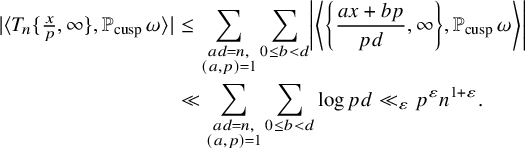 $$ \begin{align} \nonumber |\langle T_n \{\tfrac{x}{p} , \infty \}, \mathbb{P}_{\mathrm{cusp}}\, \omega \rangle| \nonumber &\leq \sum_{\substack{ad=n,\\ (a,p)=1}}\sum_{0\leq b <d} \left|\left\langle \left\{ \frac{ax+bp}{pd}, \infty \right\}, \mathbb{P}_{\mathrm{cusp}}\,\omega \right\rangle\right|\\ & \ll \sum_{\substack{ad=n,\\ (a,p)=1}}\sum_{0\leq b <d} \log pd \ll_\varepsilon p^{\varepsilon}n^{1+\varepsilon}. \end{align} $$
Here, we are using that $(ax+bp,p)=1$
, meaning that
$(ax+bp,p)=1$
, meaning that $\frac { ax+bp}{pd}$
is of the shape
$\frac { ax+bp}{pd}$
is of the shape $\gamma \infty $
for
$\gamma \infty $
for $\gamma \in \Gamma _0(p)$
with left lower entry of size
$\gamma \in \Gamma _0(p)$
with left lower entry of size $O(pd)$
. By changing contours, we have the following equality of compactly supported homology classes:
$O(pd)$
. By changing contours, we have the following equality of compactly supported homology classes:
A similar argument as above, again using Corollary 6.9, yields
 $$ \begin{align*} |\langle T_n \{\tfrac{1}{x} , \infty \}, \mathbb{P}_{\mathrm{cusp}}\, \omega \rangle|\ll_\varepsilon p^{\varepsilon}n^{1+\varepsilon}, \quad \omega\in B^\ast.\end{align*} $$
Thus, by Lemma 6.7, we conclude that
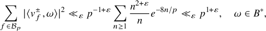 $$ \begin{align*} \sum_{f\in \mathcal{B}_p} | \langle v_f^{\pm}, \omega\rangle|^2 \ll_\varepsilon p^{-1+\varepsilon}\sum_{n\geq 1} \frac{n^{2+\varepsilon}}{n} e^{-8 n/p} \ll_\varepsilon p^{1+\varepsilon} ,\quad \omega\in B^{\ast},\end{align*} $$
as wanted.
7 The level aspect
Using the second moment bound from Theorem 6.1, we are ready to prove our main result.
Theorem 7.1. Let p be prime and let K be a real quadratic field of discriminant $d_K $
with no unit of norm
$d_K $
with no unit of norm $-1$
such that p splits in K with
$-1$
such that p splits in K with $p\mathcal {O}_K=\mathfrak {p}_1\mathfrak {p}_2$
and
$p\mathcal {O}_K=\mathfrak {p}_1\mathfrak {p}_2$
and $\mathfrak {p}_1\notin H$
where
$\mathfrak {p}_1\notin H$
where $H=(\mathrm {Cl}^+_K)^2$
.
$H=(\mathrm {Cl}^+_K)^2$
.
For ${B}$
a basic basis of level p and
${B}$
a basic basis of level p and $\omega \in B^{\ast }$
, we have
$\omega \in B^{\ast }$
, we have
 $$ \begin{align} \frac{\sum_{A\in H} \langle [\mathcal{C}_{A}(p)], \omega \rangle}{|\sum_{A\in H} \langle [\mathcal{C}_{A}(p)], \omega_{E}(p) \rangle|}= -\langle v_{E}(p), \omega\rangle+O_{\varepsilon}(d_K^{-1/12+\varepsilon}p^{2+\varepsilon}), \end{align} $$
where $v_{E}(p),\omega _{E}(p)$
denotes the Eisenstein classes in homology and cohomology as defined in (3.19) and (3.16), respectively.
$v_{E}(p),\omega _{E}(p)$
denotes the Eisenstein classes in homology and cohomology as defined in (3.19) and (3.16), respectively.
Proof. Starting from (5.6), we want to bound the cuspidal contribution on the right-hand side, which by (5.17) can be expressed in terms of L-functions. Recall that class group characters $\chi $
such that
$\chi $
such that $\chi _{|(\mathrm {Cl}_K^+)^2}$
(i.e., genus characters) correspond to factorizations
$\chi _{|(\mathrm {Cl}_K^+)^2}$
(i.e., genus characters) correspond to factorizations $d_1d_2=d_K$
in terms of fundamental discriminants, and we have
$d_1d_2=d_K$
in terms of fundamental discriminants, and we have
 $$ \begin{align*} L(\pi_f\otimes \pi_\chi,s)=L(f\otimes \chi_{d_1},s)L(f\otimes \chi_{d_2},s), \end{align*} $$
where $\chi _{d_i}=(\tfrac {d_i}{\cdot })$
are quadratic characters. Now we apply Cauchy–Schwarz followed by Hölder’s inequality with exponents
$\chi _{d_i}=(\tfrac {d_i}{\cdot })$
are quadratic characters. Now we apply Cauchy–Schwarz followed by Hölder’s inequality with exponents $(3,3,3)$
combined with Theorem 6.1 as well as the third moment bound of Petrow and Young [Reference Petrow and YoungPY19, Theorem 1]:
$(3,3,3)$
combined with Theorem 6.1 as well as the third moment bound of Petrow and Young [Reference Petrow and YoungPY19, Theorem 1]:
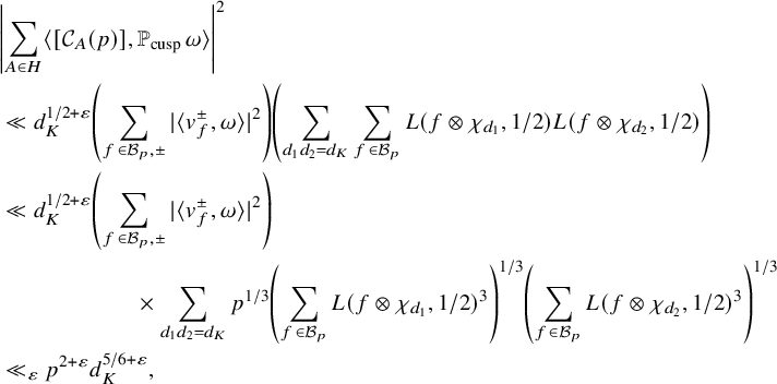 $$ \begin{align} \nonumber &\left|\sum_{A\in H} \langle [\mathcal{C}_{A}(p)], \mathbb{P}_{\mathrm{cusp}}\, \omega \rangle\right|^2\\ \nonumber&\ll d_K^{1/2+\varepsilon}\left(\sum_{f\in \mathcal{B}_p, \pm} |\langle v_f^{\pm}, \omega\rangle |^2\right) \left(\sum_{d_1d_2=d_K } \sum_{f\in \mathcal{B}_p}L(f\otimes \chi_{d_1},1/2) L(f\otimes \chi_{d_2},1/2)\right)\\ \nonumber &\ll d_K^{1/2+\varepsilon} \left(\sum_{f\in \mathcal{B}_p, \pm} |\langle v_f^{\pm}, \omega\rangle |^{2}\right) \\ &\qquad \qquad \qquad \times\sum_{d_1d_2=d_K } p^{1/3}\left(\sum_{f\in \mathcal{B}_p} L(f\otimes \chi_{d_1},1/2)^3 \right)^{1/3} \left(\sum_{f\in \mathcal{B}_p} L(f\otimes \chi_{d_2},1/2)^3 \right)^{1/3}\\ \nonumber &\ll_\varepsilon p^{2+\varepsilon} d_K^{5/6+\varepsilon} , \end{align} $$
for all $\omega \in B^{\ast }$
(using here also that
$\omega \in B^{\ast }$
(using here also that $L(f\otimes \chi _{d_i},1/2)\geq 0$
). It follows from Proposition 5.2 that the Eisenstein contribution on the right-hand side of (5.6) is
$L(f\otimes \chi _{d_i},1/2)\geq 0$
). It follows from Proposition 5.2 that the Eisenstein contribution on the right-hand side of (5.6) is $\gg _\varepsilon d_K^{1/2-\varepsilon } p^{-1}$
. Inserting all of this into (5.6) yields as wanted.
$\gg _\varepsilon d_K^{1/2-\varepsilon } p^{-1}$
. Inserting all of this into (5.6) yields as wanted.
Recall that given a basis $B\subset V_p=H_1(Y_0(p),\mathbb {R})$
, we get an associated isomorphism
$B\subset V_p=H_1(Y_0(p),\mathbb {R})$
, we get an associated isomorphism $V_p\cong \mathbb {R}^{2g+1}$
by mapping B to the standard basis of
$V_p\cong \mathbb {R}^{2g+1}$
by mapping B to the standard basis of $\mathbb {R}^{2g+1}$
. By pulling back the
$\mathbb {R}^{2g+1}$
. By pulling back the $L^r$
-norm with respect to the standard basis of
$L^r$
-norm with respect to the standard basis of $\mathbb {R}^{2g+1}$
, we get the following norm on
$\mathbb {R}^{2g+1}$
, we get the following norm on $V_p$
:
$V_p$
:
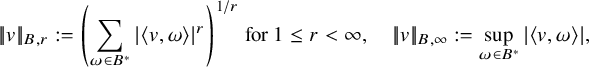 $$ \begin{align}|\!|v |\!|_{B,r}:=\left(\sum_{\omega\in B^{\ast}}|\langle v,\omega \rangle|^r\right)^{1/r}\text{ for } 1\leq r<\infty, \quad |\!|v |\!|_{B,\infty}:=\sup_{\omega\in B^{\ast}}|\langle v,\omega \rangle|, \end{align} $$
with $B^\ast \subset H^1(Y_0(p),\mathbb {R})$
the dual basis of B. Combining Theorem 7.1 and equations (5.2) and (5.4), we arrive at the following (we will skip the details).
$B^\ast \subset H^1(Y_0(p),\mathbb {R})$
the dual basis of B. Combining Theorem 7.1 and equations (5.2) and (5.4), we arrive at the following (we will skip the details).
Theorem 7.2. Let p be prime and let K be a real quadratic field of discriminant $d_K $
with no unit of norm
$d_K $
with no unit of norm $-1$
such that p splits in K with
$-1$
such that p splits in K with $p\mathcal {O}_K=\mathfrak {p}_1\mathfrak {p}_2$
and
$p\mathcal {O}_K=\mathfrak {p}_1\mathfrak {p}_2$
and $\mathfrak {p}_1\notin H$
where
$\mathfrak {p}_1\notin H$
where $H=(\mathrm {Cl}^+_K)^2$
.
$H=(\mathrm {Cl}^+_K)^2$
.
For B a basic basis of level p, we have
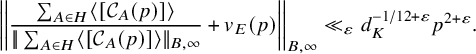 $$ \begin{align} \left| \left|\frac{\sum_{A\in H} \langle [\mathcal{C}_{A}(p)]\rangle}{|\!|\sum_{A\in H} \langle [\mathcal{C}_{A}(p)]\rangle|\!|_{B,\infty}}+v_{E}(p)\right|\right|_{B,\infty} \ll_{\varepsilon} d_K^{-1/12+\varepsilon}p^{2+\varepsilon}. \end{align} $$
8 Applications
In this section, we will present certain applications of Theorem 7.2.
8.1 A group theoretic application
Recall the independent generators of $\Gamma _0(p)$
described in Section 4.3 coming from special fundamental polygons. Given a real quadratic field K of discriminant
$\Gamma _0(p)$
described in Section 4.3 coming from special fundamental polygons. Given a real quadratic field K of discriminant $d_K $
such that p splits in K, the oriented closed geodesics
$d_K $
such that p splits in K, the oriented closed geodesics $\mathcal {C}_{A}(p)$
associated to
$\mathcal {C}_{A}(p)$
associated to $A\in \mathrm {Cl}_K^+$
corresponds to a conjugacy class of matrices inside
$A\in \mathrm {Cl}_K^+$
corresponds to a conjugacy class of matrices inside $\Gamma _0(p)$
(given by the matrices
$\Gamma _0(p)$
(given by the matrices $\gamma _Q$
defined in (3.3) where
$\gamma _Q$
defined in (3.3) where $Q\in \mathcal {Q}_{K,p}$
runs through integral binary quadratic form of discriminant
$Q\in \mathcal {Q}_{K,p}$
runs through integral binary quadratic form of discriminant $d_K $
and level p corresponding to A under the identification (3.2)). We will apply our results to understand the representation of the matrices
$d_K $
and level p corresponding to A under the identification (3.2)). We will apply our results to understand the representation of the matrices $\gamma _Q$
in terms of the independent generators (4.5) (4.6), (4.7) and (4.8) coming from a special fundamental domain of
$\gamma _Q$
in terms of the independent generators (4.5) (4.6), (4.7) and (4.8) coming from a special fundamental domain of $\Gamma _0(p)$
.
$\Gamma _0(p)$
.
Corollary 8.1. Let p be prime and let $\mathcal {P}(p)$
be a special fundamental polygon for
$\mathcal {P}(p)$
be a special fundamental polygon for $\Gamma _0(p)$
. Consider a real quadratic field K of discriminant
$\Gamma _0(p)$
. Consider a real quadratic field K of discriminant $d_K $
with no unit of norm
$d_K $
with no unit of norm $-1$
such that p splits in K with
$-1$
such that p splits in K with $p\mathcal {O}_K=\mathfrak {p}_1\mathfrak {p}_2$
and such that
$p\mathcal {O}_K=\mathfrak {p}_1\mathfrak {p}_2$
and such that $\mathfrak {p}_1 \notin (\mathrm {Cl}_K^+)^2$
. Then for
$\mathfrak {p}_1 \notin (\mathrm {Cl}_K^+)^2$
. Then for $d_K \gg _\varepsilon p^{24+\varepsilon }$
, there is some class
$d_K \gg _\varepsilon p^{24+\varepsilon }$
, there is some class $A\in (\mathrm {Cl}_K^+)^2$
such that none of the matrices
$A\in (\mathrm {Cl}_K^+)^2$
such that none of the matrices $\gamma _Q\in \Gamma _0(p)$
with
$\gamma _Q\in \Gamma _0(p)$
with $Q\in \mathcal {Q}_{K,p}$
corresponding to A are contained in the subgroup generated by the matrices in (4.6), (4.7) and (4.8).
$Q\in \mathcal {Q}_{K,p}$
corresponding to A are contained in the subgroup generated by the matrices in (4.6), (4.7) and (4.8).
Proof. Let $B_{\mathrm {sp}}\subset H_1(Y_0(p),\mathbb {R})$
be a basis obtained from the side pairing transformations of
$B_{\mathrm {sp}}\subset H_1(Y_0(p),\mathbb {R})$
be a basis obtained from the side pairing transformations of $\mathcal {P}(p)$
. Note that
$\mathcal {P}(p)$
. Note that $v_{E}(p)\in B_{\mathrm {sp}}$
and let
$v_{E}(p)\in B_{\mathrm {sp}}$
and let $\omega _0\in B_{\mathrm {sp}}^{\ast }$
be characterized by
$\omega _0\in B_{\mathrm {sp}}^{\ast }$
be characterized by $\langle v_{E}(p),\omega _0\rangle =1$
. Let
$\langle v_{E}(p),\omega _0\rangle =1$
. Let ${B}$
be a basic basis of level p containing
${B}$
be a basic basis of level p containing $v_{E}(p)$
. Then by expanding in this basis, we get by Theorem 7.2 that
$v_{E}(p)$
. Then by expanding in this basis, we get by Theorem 7.2 that
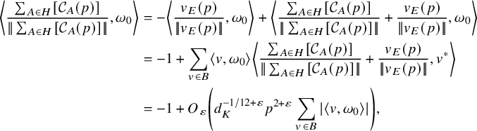 $$ \begin{align} \nonumber\left\langle \frac{\sum_{A\in H}[\mathcal{C}_{A}(p)]}{|\!|\sum_{A\in H}[\mathcal{C}_{A}(p)]|\!|} , \omega_0 \right\rangle&=-\left\langle \frac{v_{E}(p)}{|\!|v_{E}(p)|\!|}, \omega_0 \right\rangle+ \left\langle \frac{\sum_{A\in H}[\mathcal{C}_{A}(p)]}{|\!|\sum_{A\in H}[\mathcal{C}_{A}(p)]|\!|}+\frac{v_{E}(p)}{|\!|v_{E}(p)|\!|}, \omega_0 \right\rangle \\ \nonumber &=-1+\sum_{v\in B}\left\langle v, \omega_0 \right\rangle \left\langle \frac{\sum_{A\in H}[\mathcal{C}_{A}(p)]}{|\!|\sum_{A\in H}[\mathcal{C}_{A}(p)]|\!|}+\frac{v_{E}(p)}{|\!|v_{E}(p)|\!|}, v^\ast \right\rangle \\ &= -1+ O_\varepsilon\left( d_K^{-1/12+\varepsilon}p^{2+\varepsilon}\sum_{v\in B}|\langle v, \omega_0 \rangle |\right), \end{align} $$
where $|\!|\cdot |\!|=|\!|\cdot |\!|_{B,\infty }$
and
$|\!|\cdot |\!|=|\!|\cdot |\!|_{B,\infty }$
and $v^\ast \in B^\ast $
is characterized by
$v^\ast \in B^\ast $
is characterized by $\langle v, v^\ast \rangle =1$
. For
$\langle v, v^\ast \rangle =1$
. For $v\in {B}-\{v_{E}(p)\}$
, let
$v\in {B}-\{v_{E}(p)\}$
, let $\gamma _v\in \mathcal {S}(\mathcal {F}_{\mathrm {Zag}}(p))$
be such that
$\gamma _v\in \mathcal {S}(\mathcal {F}_{\mathrm {Zag}}(p))$
be such that
 $$ \begin{align*} v=\{z,\gamma_v z\}\in H_1(Y_0(p),\mathbb{R}),\end{align*} $$
using the notation (3.6) (note that the lower left entry of $\gamma _v$
is equal to p). Now for
$\gamma _v$
is equal to p). Now for $Y>0$
, consider a curve
$Y>0$
, consider a curve $c_Y: [0,1] \rightarrow \mathbb {H}$
connecting the three points
$c_Y: [0,1] \rightarrow \mathbb {H}$
connecting the three points
 $$ \begin{align*} \gamma_v^{-1} \infty +iY ,\quad \gamma_v \infty +iY,\quad \gamma_v(\gamma_v^{-1} \infty +iY)=\gamma_v\infty+ip^{-2}Y^{-1}\end{align*} $$
by a (Euclidean) straight line. We assume that Y is large enough so that
 $$ \begin{align*} \{x +iY:\min (\gamma_v\infty,\gamma_v^{-1} \infty) < x < \max(\gamma_v\infty,\gamma_v^{-1} \infty)\}\subset \mathcal{P}(p). \end{align*} $$
Observe that by Corollary 4.2, the quantity $|\langle v, \omega _0 \rangle |$
is bounded by the number of intersections between
$|\langle v, \omega _0 \rangle |$
is bounded by the number of intersections between $c_Y$
and
$c_Y$
and $\Gamma _0(p)$
-translates of
$\Gamma _0(p)$
-translates of $\{iy:y>0\}$
(which is a side of the special fundamental polygon
$\{iy:y>0\}$
(which is a side of the special fundamental polygon $\mathcal {P}(p)$
). Since
$\mathcal {P}(p)$
). Since $0<\gamma _v\infty , \gamma _v^{-1}\infty <1$
, there is no such intersection for the horizontal segment of
$0<\gamma _v\infty , \gamma _v^{-1}\infty <1$
, there is no such intersection for the horizontal segment of $c_Y$
. Intersections with the vertical segment correspond to integers
$c_Y$
. Intersections with the vertical segment correspond to integers $a,b,c,d$
such that
$a,b,c,d$
such that
 $$ \begin{align}p|c,\qquad ad-bc=1,\qquad\text{and}\quad \frac{a}{c}<\gamma_v\infty <\frac{b}{d}\text{ or }\frac{b}{d}<\gamma_v\infty <\frac{a}{c}.\end{align} $$
In particular, we have $\gamma _v\neq \frac {a}{c}$
, which implies
$\gamma _v\neq \frac {a}{c}$
, which implies
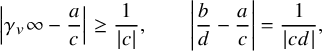 $$ \begin{align*} \left|\gamma_v\infty-\frac{a}{c}\right|\geq \frac{1}{|c|},\qquad \left|\frac{b}{d}-\frac{a}{c}\right|=\frac{1}{|cd|},\end{align*} $$
but this contradicts (8.2). This implies that $\langle v, \omega _0 \rangle =0$
for
$\langle v, \omega _0 \rangle =0$
for $v\in {B}-\{v_{E}(p)\}$
which by (8.1) yields the wanted error-term.
$v\in {B}-\{v_{E}(p)\}$
which by (8.1) yields the wanted error-term.
From the above, Corollary 1.7 follows in the case where K has wide class number one and narrow class number two by writing out explicitly the matrices $\gamma _Q$
associated to
$\gamma _Q$
associated to $Q\in \mathcal {Q}_{K,p}$
as in (3.3) and recalling that since K does not have a unit of norm
$Q\in \mathcal {Q}_{K,p}$
as in (3.3) and recalling that since K does not have a unit of norm $-1$
, the condition
$-1$
, the condition $\mathfrak {p}_1 \notin (\mathrm {Cl}_K^+)^2$
is equivalent to
$\mathfrak {p}_1 \notin (\mathrm {Cl}_K^+)^2$
is equivalent to $\mathfrak {p}_1$
not having a generator of positive norm.
$\mathfrak {p}_1$
not having a generator of positive norm.
8.2 An application to modular forms
Recall the following definition mentioned in the introduction for a modular form $f\in \mathcal {M}_2(p)$
:
$f\in \mathcal {M}_2(p)$
:
 $$ \begin{align*} M_{f}:=\inf \{c\geq 0: |a_f(n)|\leq c \sigma_1(n) ,\, n\geq 1\}<\infty, \end{align*} $$
where $a_f(n)$
denotes the Fourier coefficients of f (at
$a_f(n)$
denotes the Fourier coefficients of f (at $\infty $
) and
$\infty $
) and $\sigma _1(n)=\sum _{d|n}d$
. We have the following nonvanishing result for cycle integrals of modular forms.
$\sigma _1(n)=\sum _{d|n}d$
. We have the following nonvanishing result for cycle integrals of modular forms.
Corollary 8.2. Let p be prime and let $f\in \mathcal {M}_2(p)$
be a holomorphic modular form of weight
$f\in \mathcal {M}_2(p)$
be a holomorphic modular form of weight $2$
and level p with constant Fourier coefficient equal to
$2$
and level p with constant Fourier coefficient equal to $a_f(0)=1$
. Consider a real quadratic field
$a_f(0)=1$
. Consider a real quadratic field $K$
of discriminant
$K$
of discriminant $d_K$
with no unit of norm
$d_K$
with no unit of norm $-1$
such that
$-1$
such that $p$
splits in
$p$
splits in $K$
with
$K$
with $p\mathcal{O}_K=\mathfrak{p}_1\mathfrak{p}_2$
and
$p\mathcal{O}_K=\mathfrak{p}_1\mathfrak{p}_2$
and $\mathfrak{p}_1 \notin (\mathrm{Cl}_K^+)^2$
. Then for
$\mathfrak{p}_1 \notin (\mathrm{Cl}_K^+)^2$
. Then for $d_K \gg_\varepsilon (M_{f})^{12+\varepsilon} p^{48+\varepsilon}$
there is some
$d_K \gg_\varepsilon (M_{f})^{12+\varepsilon} p^{48+\varepsilon}$
there is some $A\in (\mathrm{Cl}_K^+)^2$
such that
$A\in (\mathrm{Cl}_K^+)^2$
such that
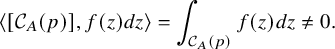 $$ \begin{align*}\langle [\mathcal{C}_{A}(p)], f(z)dz\rangle= \int_{\mathcal{C}_{A}(p)} f(z)dz\neq 0.\end{align*} $$
Proof. Let
 $$ \begin{align*} f(z)dz= \omega_+ +i\omega_-\in H^1(Y_0(p),\mathbb{R})\oplus i H^1(X_0(p),\mathbb{R}) \end{align*} $$
be the cohomology class (with complex coefficients) associated to f. By expanding in a basic basis $B\subset H_1(Y_0(p),\mathbb {R})$
as in (8.1) and using Cauchy–Schwarz followed up by (7.4), we conclude that
$B\subset H_1(Y_0(p),\mathbb {R})$
as in (8.1) and using Cauchy–Schwarz followed up by (7.4), we conclude that
 $$ \begin{align*} \left|\left\langle \frac{\sum_{A\in H}[\mathcal{C}_{A}(p)]}{|\!|\sum_{A\in H}[\mathcal{C}_{A}(p)]|\!|_{B,\infty}}-v_{E}(p) , \omega_\pm \right\rangle\right|\ll_\varepsilon p^{3+\varepsilon} d_K^{-1/12+\varepsilon}\sup_{v\in {B}}|\langle v, \omega_\pm \rangle |. \end{align*} $$
Now by the assumptions on the Fourier expansion of f, we get
 $$ \begin{align*} f(x+iy)&\ll 1+ M_{f}\sum_{n\geq 1}\sigma_1(n) e^{-2\pi yn}\ll_\varepsilon 1+M_{f}\int_1^\infty t^{1+\varepsilon} e^{-2\pi ty} \frac{dt}{t}\ll_\varepsilon \mathrm{max} (1, M_{f} y^{-1-\varepsilon}). \end{align*} $$
In order to bound the quantities $\langle v, \omega _\pm \rangle $
for
$\langle v, \omega _\pm \rangle $
for $v\in {B}$
, we recall that we can write
$v\in {B}$
, we recall that we can write $v=\{\gamma z, z\}$
for
$v=\{\gamma z, z\}$
for $z\in \mathbb {H}$
(which we may choose freely) and some matrix
$z\in \mathbb {H}$
(which we may choose freely) and some matrix
![]() as in Section 4.2. In particular, we observe that by construction, we have
as in Section 4.2. In particular, we observe that by construction, we have $a,b,c,d\ll p$
and
$a,b,c,d\ll p$
and $ c\in \{ 0,p\}$
. If
$ c\in \{ 0,p\}$
. If $c=0$
, then clearly
$c=0$
, then clearly $ \langle v, \omega _\pm \rangle \in \{0,1\}$
. If
$ \langle v, \omega _\pm \rangle \in \{0,1\}$
. If $c=p$
, we make the following convenient choice
$c=p$
, we make the following convenient choice $z=\frac {-d}{p}+\frac {i}{p}$
satisfying
$z=\frac {-d}{p}+\frac {i}{p}$
satisfying $\gamma z=\frac {a}{p}+\frac {i}{p}$
. This gives
$\gamma z=\frac {a}{p}+\frac {i}{p}$
. This gives
 $$ \begin{align*} \langle v, \omega_\pm \rangle= \int_{\tfrac{a}{p}}^{-d/p} \frac{f(x+ip^{-1})\pm \overline{f(x+ip^{-1})}}{2i^{(1\mp 1)/2}} dx\ll_\varepsilon M_{f} \frac{|a+d|}{p}p^{1+\varepsilon}\ll_\varepsilon M_{f} p^{1+\varepsilon},\end{align*} $$
which we plug into the above. Since $\langle v_{E}(p),\omega _+ \rangle =1$
and
$\langle v_{E}(p),\omega _+ \rangle =1$
and $\langle v_{E}(p),\omega _- \rangle =0$
, we conclude that
$\langle v_{E}(p),\omega _- \rangle =0$
, we conclude that $\langle \sum _{A\in H}[\mathcal {C}_{A}(p)] , f(z)dz \rangle $
is indeed nonvanishing for
$\langle \sum _{A\in H}[\mathcal {C}_{A}(p)] , f(z)dz \rangle $
is indeed nonvanishing for $d_K \gg _\varepsilon (M_{f})^{12+\varepsilon } p^{48+\varepsilon }$
, as wanted.
$d_K \gg _\varepsilon (M_{f})^{12+\varepsilon } p^{48+\varepsilon }$
, as wanted.
Now Corollary 1.8 follows from the above in the case of wide class number one and narrow class number two.
Acknowledgements
The author would like to thank Peter Humphries, Raphael Steiner, Daniel Kriz and Farrell Brumley for useful discussions. The author would also like to thank the referee for a careful and insightful reading with many valuable suggestions, as well as pointing out a mistake in a key step of an earlier version of the proof of the main result.
Competing interest
The author have no competing interest to declare.
Funding statement
This research was supported by a grant from the Independent Research Fund Denmark DFF(1025-00020B).


 Open access