


1. Introduction
1.1. Brief review of minimum-enstrophy vortex and maximum-entropy theories in 2-D fluids
In homogeneous incompressible fluids, free-decay two-dimensional (2-D) turbulence is characterized by the spontaneous appearance of vortices which grow by merging with their homostrophic partners, and shed filaments to conserve angular momentum during the merging events (McWilliams Reference McWilliams1984, Reference McWilliams1990b). This increase in vortex sizes is the physical manifestation of the upscale cascade of energy in wavenumber space, while the production of thin filaments is associated with the downscale cascade of enstrophy (variance of vertical vorticity). While kinetic energy is only weakly (or not) dissipated at large scales, enstrophy is erased by viscosity at the dissipation wavenumber that often corresponds to the numerical grid size in simulations. In the absence of forcing, dissipation, bottom topography and beta effect, the final state of such a turbulent flow is a pair of contra-rotating vortices. The search for the spatial structure of final vortex states in 2-D turbulence has motivated the original work on minimum-enstrophy vortices (hereafter MEVs) (Leith Reference Leith1984a,Reference Leithb), and more recently, a search for exact coherent structures in 2-D turbulent flows (Zhigunov & Grigoriev Reference Zhigunov and Grigoriev2023). In his seminal paper, Leith used variational principles to derive the velocity profile of an axisymmetric vortex in 2-D incompressible flows, with minimal enstrophy for a given energy, angular momentum or circulation. He found two different MEVs, one with finite angular momentum (MEV M), one with finite circulation (MEV C), both described by Bessel functions of the radius.
In conclusion, Leith mentioned that final states in numerical simulations of 2-D turbulence may look more like MEV C than MEV M. Furthermore, his MEVs were barotropically unstable to small-scale perturbations, leading to non-axisymmetric (tripolar) vortices with even lower enstrophy.
Further work was done by Kozlov (Reference Kozlov1994), studying the compensated MEV, that is a MEV with different vorticity distributions,  $q$, in the core and in the periphery; he studied a non-axisymmetric vortex. But this MEV had a piecewise-constant vorticity distribution and not a continuously distributed one. Later, efforts to calculate tripolar MEVs in 2-D flows, with continuous vorticity distributions, and having a linear vorticity–streamfunction relation, were not successful. Furthermore, numerical experiments suggested that steady tripolar states have nonlinear $q-\psi$ relations, with $\psi$ the streamfunction. Theoretical work done with such nonlinear $q-\psi$ relations also had to deal with critical layers, leading to very complex algebra.
Approaching the final state of free-decay 2-D turbulence from a statistical mechanics point of view, Smith (Reference Smith1991) determined that the squared-Lorentzian vortex  $\nabla ^2 \psi (r) = \zeta _0 / [1+ (r/r_0)^2]^2$, with $\zeta_0$ the amplitude, r the radial coordinate and $r_0$ the characteristic radius, was an exact solution to the mean field theory.
Huang & Driscoll (Reference Huang and Driscoll1994) reported an experiment showing that mixing is not very well realized in the core of the vortex. Their experiment was based on an electron plasma confined by a magnetic field. For high values of the magnetic field, the time evolution of the electron density becomes equivalent to the Euler dynamics of the vorticity and a quasi-inviscid flow is produced. Huang and Driscoll studied the relaxation of an initial hollow column of electrons towards an axisymmetric meta-equilibrium state and compared their result with existing theories of 2-D almost inviscid fluid dynamics. They claimed that their equilibrium density vorticity profile exhibited close agreement with a MEV restricted to a subdomain to avoid spurious negative vorticity values but differed substantially from maximum-entropy predictions.
Further work was done using the statistical theory. Chavanis & Sommeria (Reference Chavanis and Sommeria1996, Reference Chavanis and Sommeria1998) solved the 2-D Euler equations in the limit of the statistical theory where maximum-entropy states are equivalent to minimum-enstrophy states and proposed a convenient classification of the maximum-entropy states for bounded and unbounded domain.
Motivated by the experiments of Huang & Driscoll (Reference Huang and Driscoll1994), Brands et al. (Reference Brands, Chavanis, Pasmanter and Sommeria1999) compared vortex structures having maximal entropy with those having minimal enstrophy. They described the minimum-enstrophy principle as an approximation of the statistical theory. In the case investigated by Huang and Driscoll, they claimed that this approximation even yielded a better agreement with experiments than the full statistical theory because the relaxation of the system toward the maximum-entropy state was not complete. However, they emphasized the problem of spurious negative oscillations and explained that this agreement cannot hold in more general cases. Nevertheless, they concluded that when relaxing the angular momentum constraint, enstrophy minimization was consistent with the physics of the system except near the maximum accessible energy. Therefore, the MEV remained a useful solution for the statistical theory of the Euler equation, except at high energy.
1.2. Motivation for the work
Following the review in § 1.1 the MEV's ability to represent axisymmetric coherent vortices in 2-D turbulence has been debated. However, two aspects have been left untouched.
First, non-axisymmetric 2-D MEVs with continuous vorticity distributions have never been studied; this is important since vortices are rarely axisymmetric. This point will deserve a future study.
Second, a generalization to the continuously stratified three-dimensional (3-D) geostrophic turbulence including vortex stretching remains to be done. In 3-D geostrophic turbulence, according to Charney's work (Charney Reference Charney1971), the energy is equipartitioned horizontally and vertically (between kinetic and potential components). This can lead to isotropic vortex structures (McWilliams, Weiss & Yavneh Reference McWilliams, Weiss and Yavneh1991).
Following this statement, we look for isotropic vortices, minimizing potential enstrophy with given total energy and generalized momentum. This is in accordance with the cascades of geostrophic turbulence, associated with horizontal and vertical growth of the vortices and with the formation of small-scale filaments, containing a substantial amount of potential enstrophy, and which are dissipated by viscosity (Rhines Reference Rhines1979; McWilliams Reference McWilliams1989, Reference McWilliams1990a). Providing the 3-D structure of such MEVs and assessing their robustness are the aim of the present article.
The article is organized as follows. The first part is dedicated to the methodology to construct the functional to minimize, including the calculation of enstrophy and global invariants such as energy, momentum and Casimir's. In the second part, the calculus of variations and the solution are obtained and are discussed. Finally, we assess numerically the stability and evolution of such 3-D MEVs.
2. Methodology
Considering rotating stratified flows, we work in the framework of the continuously stratified quasi-geostrophic (QG) equations (Charney Reference Charney1948; Charney & Phillips Reference Charney and Phillips1953). The equations require two conditions to be satisfied by the flow: a small Rossby number ( $Ro= V/(f_0 R)$) and an order-one Burger number ( $Bu = (N H/(f_0 R))^2 \sim 1$), where $N(Z)$ and $f_0$ are the stratification frequency and the Coriolis parameter, $H$ and $R$ are the vertical and horizontal scales of the vortex ( $Z$ is the vertical coordinate) and V the maximum velocity of the flow. In the absence of forcing and of dissipation, the QG model is governed by the equation of potential vorticity conservation:
 \begin{equation} \left.\begin{array}{c@{}} D_t q=0, \\ q = (\partial_x^2 + \partial_y^2) \psi + \partial_Z \left(\dfrac{f_0^2}{N^2(Z)} \partial_Z \psi\right), \\ D_t = \partial_t + u_g \partial_x + v_g \partial_y, \end{array}\right\} \end{equation}
with  $(u_g=-\partial _y \psi,v_g=\partial _x \psi )$ the horizontal geostrophic velocities. Usually, we apply the boundary conditions $\partial _Z \psi (Z=0, -H)=0$. In the special case of constant stratification (that we consider here) $N(Z)=N_0$, and using the constraint on $Bu$, we can rescale the vertical coordinate $Z$ via $z=N_0 Z/f_0$ and the relation between the potential vorticity and the streamfunction becomes $q = (\partial _x^2 + \partial _y^2 + \partial _z^2) \psi = \nabla ^2 \psi$. In these coordinates, the potential vorticity is simply the Laplacian of the streamfunction.
We define a 3-D (local) radius  $r^2 = x^2 + y^2 + z^2$ and finally, we scale again it by the vortex radius $s=r/R$. We also define a 2-D radius via $\rho ^2=x^2+y^2$ scaled as $\sigma =\rho /R$. In this spherical frame of reference, $\theta$ and $\phi$ respectively refer to the latitude (positive towards the North) and the longitude (positive towards the West).
Our goal is to find a spherically symmetric vortex in the QG model, satisfying a minimal enstrophy constraint while energy (and possibly other integral quantities) is prescribed. Our vortex should have a finite extent. Therefore, we assume that the potential vorticity is zero beyond a radius  $R$. Thus, for $r > R$, that is for $s > 1$, we have $\nabla ^2_s \psi = 0 = \frac {1}{s^2} \ \partial _s (s^2 \partial _s \psi )$ where $\nabla ^2_s = ({1}/{s^2}) \partial _s (s^2 \partial _s)$ is the non-dimensional Laplacian, leading to a solution $\psi (s>1)=K/s$, with $K$ a constant to be determined from continuity of the velocity field at $s=1$.
We next determine the internal structure of the vortex (for  $s<1$). We first list the integral invariants of the unforced, non-dissipative QG equations, in order to build the functional of streamfunction $F(\psi )$ the extremum of which we wish to determine. Let us define $Z$ the enstrophy, $E$ the energy and $L = \int \rho ^2 q \, \textrm {d}V$ the angular momentum with the horizontal radius $\rho = R s \cos (\theta )$ as well as the associated non-dimensional quantities $\hat {Z}$, $\hat {E}$ and $\hat {L}$. We also define the non-dimensional streamfunction $\hat {\psi }$ such that $\psi =\varPsi \hat {\psi }$, with $\varPsi$ the scale of the streamfunction. We write
 \begin{align} \left.
\begin{array}{@{}c@{}} \displaystyle \hat{Z} =
\dfrac{R}{\varPsi} Z = 2 {\rm \pi}\int_0^1 s^2 (\nabla_s^2
\hat{\psi})^2 \, {\rm d}s, \\ \displaystyle \hat{E} =
\dfrac{E}{R \varPsi^2} = 2 {\rm \pi}\int_0^1 s^2 |\boldsymbol{\nabla}_s
\hat{\psi}|^2 \, {\rm d}s =2 {\rm \pi}\int_0^1 s^2 ({\rm
d}\hat{\psi}/{\rm d}s)^2 \,{\rm d}s, \\ \displaystyle
\hat{L} = \dfrac{L}{R^3 \varPsi} = \dfrac{8 {\rm \pi}}{3}
\int_0^1 \nabla_s^2 \hat{\psi} s^4 \, {\rm d}s.
\end{array}\right\} \end{align}
\begin{align} \left.
\begin{array}{@{}c@{}} \displaystyle \hat{Z} =
\dfrac{R}{\varPsi} Z = 2 {\rm \pi}\int_0^1 s^2 (\nabla_s^2
\hat{\psi})^2 \, {\rm d}s, \\ \displaystyle \hat{E} =
\dfrac{E}{R \varPsi^2} = 2 {\rm \pi}\int_0^1 s^2 |\boldsymbol{\nabla}_s
\hat{\psi}|^2 \, {\rm d}s =2 {\rm \pi}\int_0^1 s^2 ({\rm
d}\hat{\psi}/{\rm d}s)^2 \,{\rm d}s, \\ \displaystyle
\hat{L} = \dfrac{L}{R^3 \varPsi} = \dfrac{8 {\rm \pi}}{3}
\int_0^1 \nabla_s^2 \hat{\psi} s^4 \, {\rm d}s.
\end{array}\right\} \end{align}
Using the radial Laplacian only is justified since  $\hat {\psi }$ must not depend on the spherical angles for a centrally symmetric vortex in 3-D. Finally, there is an infinity of Casimir invariants for the unforced, non-dissipative QG equations, among which are the potential vorticity integral $C$ (and its non-dimensional form $\hat {C}$):
 \begin{equation} \hat{C} = \frac{C}{R \varPsi} = 4 {\rm \pi}\int_0^1 s^2 (\nabla_s^2 \hat{\psi}) \, {\rm d}s. \end{equation}
Nevertheless, it should be noted that, if the vortex is isolated (that is, if it does not advect the whole fluid in rotation), this last integral must vanish. In the following, we drop the hat for non-dimensional quantities.
Following Leith (Reference Leith1984b), we could have performed variations of the functional  $F(\psi )$ with respect to the vortex radius $R$, but this would have led to a relation between the Lagrange multipliers, and the enstrophy that we minimize (which is therefore unknown). We refer the reader to Appendix A for more details.
Therefore, we choose the functional to be varied with respect to  $\psi$:
 \begin{equation} F(\psi) = Z(\psi) - \lambda E(\psi) - \mu L(\psi), \end{equation}
with  $C(\psi )=0$, $\mu$ and $\lambda$ two Lagrange multipliers. Physically, and mathematically as we will see below, this leads to $K=0$ for the external solution.
3. Calculus of variation and the solution
To calculate a variation of  $F$ with respect to $\psi$ we need to have $\delta \psi$ to appear explicitly in the expressions of $\delta Z, \delta E, \delta L$, where $\delta$ denotes the variation of the quantity. To do so, we will perform integrals by parts. Again, remember that we work in spherically symmetric (3-D) configuration, using the scaled spherical radius $s$.
$s$.
3.1. First-order variation
Before we calculate these part integrals, we make explicit the condition  $C=0$. Integrating using the expression of the 3-D radial Laplacian in $s$ leads simply to $\textrm {d}\psi /\textrm {d}s(s=1)=0$. This condition will be used later in the calculation.
Now, we calculate  $\textrm {d}F/\textrm {d}\psi \delta \psi$ by integration by parts for the enstrophy, energy and momentum. For these integrations by parts, we have the usual conditions $\delta \psi =0$ in $s=0,1$. We have successively the enstrophy, energy and momentum variations:
 \begin{equation} \left.
\begin{array}{@{}c@{}} \displaystyle \delta Z = 4 {\rm \pi}
\int_0^1 \nabla_s^2 q \delta \psi s^2 \, {\rm d}s, \\
\displaystyle - \lambda \delta E = 4 {\rm \pi}\lambda \int_0^1 q
\delta \psi s^2 \, {\rm d}s, \\ \displaystyle - \mu \delta
L ={-} 16 {\rm \pi}\mu \int_0^1 \delta \psi s^2 \, {\rm d}s.
\end{array}\right\} \end{equation}
\begin{equation} \left.
\begin{array}{@{}c@{}} \displaystyle \delta Z = 4 {\rm \pi}
\int_0^1 \nabla_s^2 q \delta \psi s^2 \, {\rm d}s, \\
\displaystyle - \lambda \delta E = 4 {\rm \pi}\lambda \int_0^1 q
\delta \psi s^2 \, {\rm d}s, \\ \displaystyle - \mu \delta
L ={-} 16 {\rm \pi}\mu \int_0^1 \delta \psi s^2 \, {\rm d}s.
\end{array}\right\} \end{equation}
Therefore, cancelling the whole variation of  $F$ at first order in $\delta \psi$ (to obtain an extremum of $F$) leads to
 \begin{equation} \nabla_s^2 q + \lambda q - 4 \mu = 0. \end{equation}
This equation has a special solution satisfying both  $q=4 \mu / \lambda$ and $\nabla _s^2 q = 0$ simultaneously. This special solution is written as
 \begin{equation} \psi_s = \psi_2 + \frac{2 \mu}{3 \lambda} s^2 = \psi_2 + \psi_1 s^2, \end{equation}
where  $\psi _2$ is a constant, and $\psi _1 = 2\mu /(3\lambda )$. Then, we have to solve the homogeneous rest of the first-order equation $\nabla _s^2 q + \lambda q = 0$. The general solution of which is
 \begin{equation} q_g (s) = q_0 \, j_0 (\sqrt{\lambda} s), \end{equation}
where  $j_0(x)= \sin (x)/x=\textrm {sinc}(x)$ is the zeroth-order spherical Bessel function. For a 2-D configuration, Leith (Reference Leith1984) found a general solution as a function of the first-order standard Bessel function but he calculated the functional variation according to the velocity instead of the streamfunction. Considering our geometrical hypothesis, our expression is consistent with his. Finally, we have the complete solution:
 \begin{equation} \psi(s) = \psi_0 \, j_0(\sqrt{\lambda} s)+ \psi_1 s^2 + \psi_2, \end{equation}
where we have three unknowns  $\psi _0$, $\mu$, $\lambda$, since $\psi _1$ is expressed as a function of $\mu$ and $\lambda$. As the streamfunction is defined to a constant, $\psi _2$ does not count as an unknown. However, we have to make a choice as we actually have four constraints:
(i) the boundary condition: $q(1) = \nabla _s^2 \psi (s=1)=0$,
(ii) the potential vorticity:
$\textrm {d}\psi /\textrm {d}s(s=1)=0$,(iii) the prescribed energy:
$E=E_0$,(iv) the prescribed momentum:
$L=L_0$.


Leaving for now the first condition, accounting only for the three last conditions and after some long algebra, we obtain three equations (written in the same order as the constraints).
 \begin{equation} \left.\begin{array}{@{}c@{}} \displaystyle \psi_1 = \dfrac{2 \mu}{3 \lambda} = \dfrac{\sqrt{\lambda}}{2} j_1(\sqrt{\lambda}) \psi_0,\\ \displaystyle L_0 = \dfrac{16 {\rm \pi}}{15} \sqrt{\lambda} j_1(\sqrt{\lambda}) \left( \dfrac{5}{\sqrt{\lambda}} \dfrac{j_2(\sqrt{\lambda})}{j_1(\sqrt{\lambda})} - 1 \right) \psi_0,\\ \displaystyle E_0 = \dfrac{7 {\rm \pi}}{5} \lambda j_1^2(\sqrt{\lambda}) \left(1 - \dfrac{25}{7\sqrt{\lambda}} \dfrac{j_2(\sqrt{\lambda})}{j_1(\sqrt{\lambda})} + \dfrac{5}{7} \dfrac{j_2^2(\sqrt{\lambda})}{j_1^2(\sqrt{\lambda})} \right) \psi_0^2, \end{array}\right\} \end{equation}
where  $j_1$ and $j_2$ are spherical Bessel functions of order one and two, respectively. Calculations have mostly been done using the results of Bloomfield, Face & Moss (Reference Bloomfield, Face and Moss2017) which performed some analytical derivations on spherical Bessel functions.
Now the issue is to isolate the unknowns so as to determine them, which is not that easy as the system is nonlinear. In 2-D, the variation of the functional according to the vortex radius gave a simple relation between  $E_0$ and $L_0$ in order to determine $\lambda$. In all cases, the energy must be positive and by similarity to the 2-D case (where $\lambda$ was the solution of $J_2(\sqrt {\lambda })=0$, where $J_2$ was the second-order standard Bessel function), we can set $\lambda$ as a solution of $j_2(\sqrt {\lambda })=0$. Therefore, we have $\sqrt {\lambda }=\gamma _n$ for some $n=1,2,\ldots\,$. It is worth noting that setting this constraint makes both conditions $q(1)=0$ and $\textrm {d}\psi /\textrm {d}s(s=1)=0$ equivalent. Therefore, the continuity with the external problem is also verified.
In that case, the system is reduced to
 \begin{equation} \left.\begin{array}{@{}c@{}} \displaystyle \psi_1 = \dfrac{2 \mu}{3 \lambda} = \dfrac{\sqrt{\lambda}}{2} j_1(\sqrt{\lambda}) \psi_0, \\ \displaystyle L_0 ={-}\dfrac{16 {\rm \pi}}{15} \sqrt{\lambda} j_1(\sqrt{\lambda}) \psi_0, \\ \displaystyle E_0 = \dfrac{7 {\rm \pi}}{5} \lambda j_1^2(\sqrt{\lambda}) \psi_0^2. \end{array}\right\} \end{equation}
As in the 2-D case of Leith (1984),  $L_0$ and $E_0$ are thus linked, here, through the relation ${L_0^2}/{E_0} = \frac {256}{315} {\rm \pi}$; $\psi _0$ and $\mu$ are thus given by $\psi _0 = -({16}/{21 \sqrt {\lambda } j_1(\sqrt {\lambda })}) ({E_0}/{L_0})$ and $\mu = -\frac {4}{7} \lambda ({E_0}/{L_0})$.
With these considerations, using  $r_h = R \sigma$, this streamfunction leads to an azimuthal velocity:
 \begin{equation} V(s) = \frac{\partial \psi}{\partial \sigma} = \frac{16}{21} \left( \frac{E_0}{L_0} \right) \frac{1}{j_1(\sqrt{\lambda})} (j_1(\sqrt{\lambda} s) - j_1(\sqrt{\lambda})s ) \cos{\theta}, \end{equation}
using the fact that  $\textrm {d}s/\textrm {d}\sigma =\sigma /s= \cos (\theta )$. This expression is similar to equation (34) by Leith (1984). Therefore, the velocity field is maximum for $\theta =0$, the median plane of the vortex, and minimum for $\theta =\pm {{\rm \pi} }/{2}$, at the top and bottom of the vortex.
3.2. Second-order variation
Following Leith (1984), the second variation analysis needs to assure that one of the stationary solutions already found is a true minimum. This approach is more easily carried out using a spectral representation. In this part, calculus will be performed using  $\textrm {d} \psi /\textrm {d}s$ instead of $\psi$ as it leads to simpler expressions. Initially, the aim was to show that $\textrm {d}F/\textrm {d}\psi =0$ and $\textrm {d}^2F/\textrm {d}\psi ^2>0$ with $F$ previously defined. Then, we slightly change our problem to $\textrm {d}F/\textrm {d}u=0$ and $\textrm {d}^2F/\textrm {d}u^2>0$ with $u=\textrm {d}\psi /\textrm {d}s$. The important thing is to show both conditions with the same variable. Replacing $\psi$ by $u$ in the second-order derivative is not simple but doable. However, replacing in the first-order derivative remains easy. Indeed, if $\textrm {d}F/\textrm {d}\psi =0$ then $\textrm {d}F/\textrm {d}u = (\textrm {d}F/\textrm {d}\psi )(\textrm {d}\psi /\textrm {d}u)=0$. Using the properties of $\gamma _n$, $\textrm {d}\psi /\textrm {d}s$ can be represented in terms of coefficients $A_n$ in the series
 \begin{equation} \frac{{\rm d}\psi}{{\rm d}s} = \sum_{n=0}^{\infty} A_n g_n(s), \end{equation}
where the basis functions are defined by  $g_0(s) = \sqrt {5} s$ and $g_n(s) = \sqrt {2} (\,{j_1(\gamma _n s)}/{j_1(\gamma _n)}) \ \textrm {for} n=1,2, \ldots$ so that the following orthonormality relation is satisfied:
 \begin{equation} \int_0^1 s^2 g_n(s) g_m(s) \,{\rm d}s = \delta_{nm} \quad \text{for} \ 0 \leq n,m < \infty, \end{equation}
when  $j_2(\gamma _n)=0$ for $n=1,2,\ldots\,$. Then, we can derive the Laplacian of the streamfunction such that
 \begin{equation} \nabla^2_s\psi = \sum_{n=0}^{\infty} A_n h_n(s), \end{equation}
where we have  $h_0(s) = 3\sqrt {5}$ and $h_n(s) = 3\sqrt {2} (\,{j_0(\gamma _n s)}/{j_0(\gamma _n)}) \ \textrm {for} \ n=1,2, \ldots\,$. Note that these functions are not orthogonal. The condition on the potential vorticity of an isolated vortex imposes a linear constraint on the coefficients $A_n$ such that $\sqrt {5} A_0 + \sqrt {2} \sum _{n=1}^{\infty } A_n = 0$. Finally, using this condition and (3.11), the angular momentum, the energy and the enstrophy are
 \begin{equation} \left. \begin{array}{@{}c@{}} \displaystyle L = \dfrac{8 {\rm \pi}}{3} (\sqrt{2}-\sqrt{5}) A_0, \\ \displaystyle E = 2{\rm \pi} \sum_{n=1}^{\infty} A_n^2, \\ \displaystyle Z = 2 {\rm \pi}\sum_{n,m=0}^{\infty} H_{mn} A_n A_m, \end{array}\right\} \end{equation}
where  $H_{mn} = \int _0^1 s^2 h_m(s) h_n(s) \,\textrm {d}s$. Then, using again the results from Bloomfield et al. (Reference Bloomfield, Face and Moss2017) on integrals of spherical Bessel functions, one can find the explicit expression for $H_{mn}$ as follows: $H_{00} = 15$, $H_{n0} = H_{0n} = 3 \sqrt {10}$, $H_{nn} = 6 + \gamma _n^2 \ \textrm {for} \ n=1,2, \ldots$ and $H_{mn} = 6\ \textrm {for} \ n,m=1,2,\ldots\,$.
By substituting the previous constraint on  $A_n$ coefficients into the enstrophy expression, we end up with
 \begin{equation} Z = 2 {\rm \pi}\sum_{n=1}^{\infty} \gamma_n^2 A_n^2. \end{equation}
Therefore, using (3.11) we can write  $A_0$ as a function of $L$ and express the energy and enstrophy. That leads to $A_0 = {3 L}/{8 {\rm \pi}(\sqrt {2}-\sqrt {5})}$, $E = ({9 L^2}/{32 {\rm \pi}(\sqrt {2}-\sqrt {5})^2}) (1 + \sum _{n=1}^{\infty } B_n^2 )$ and $Z = ({9 L^2}/{32 {\rm \pi}(\sqrt {2}-\sqrt {5})^2}) \sum _{n=1}^{\infty } \gamma _n^2 B_n^2$ with $B_n = A_n/A_0$. Therefore, in spectral representation, the first-order variations of $E$ and $Z$ are straightforward and the constrained first variation equation becomes
 \begin{equation} \delta Z - \lambda \delta E = \frac{9 L^2}{16 {\rm \pi}(\sqrt{2}-\sqrt{5})^2} \sum_{n=1}^{\infty} (\gamma_n^2 - \lambda) (\delta B_n) B_n = 0. \end{equation}
This equation may be satisfied for all  $\delta B_n$ which leads to $\gamma _N^2 = \lambda$, for $N=1,2,\ldots\,$. In particular, the constraints on $A_n$ coefficients leads to $B_N=-\sqrt {5/2}$ and we have $B_n=0$ for $0< n\neq N$. We thus have $E = {63 L^2}/{64 {\rm \pi}(\sqrt {2}-\sqrt {5})^2}$ and $Z = ({45 L^2}/{64 {\rm \pi}(\sqrt {2}-\sqrt {5})^2}) \gamma _N^2$.
Of these various stationary solutions, the most important one with  $N=1$ has the smallest value of $Z$ since $\gamma _1^2<\gamma _2^2<\gamma _3^2<\cdots$. But to assure ourselves that it is a true minimum in $Z$, we must examine the second variation. The combined second variation about the stationary solution of interest becomes for $N=1$
$N=1$
 \begin{equation} \delta^2 Z - \lambda \delta^2E = \frac{9 L^2}{16 {\rm \pi}(\sqrt{2}-\sqrt{5})^2} \sum_{n=2}^{\infty} (\gamma_n^2 - \gamma_1^2) (\delta B_n)^2. \end{equation}
Since  $\gamma _1^2<\gamma _2^2<\gamma _3^2<\cdots$, this second variation is positive for any $\delta B_n$. The solution is thus a true minimum.
3.3. Solution
Finally, for  $N=1$ that minimizes the enstrophy value, the azimuthal velocity and the potential vorticity field are
 \begin{equation} \left. \begin{array}{@{}c@{}} \displaystyle V(s)= \dfrac{16}{21} \left( \dfrac{E_0}{L_0} \right) \dfrac{1}{j_1(\gamma_1)} (j_1(\gamma_1 s) - j_1(\gamma_1)s ) \cos{\theta}, \\ \displaystyle q(s)= \dfrac{16}{7} \left( \dfrac{E_0}{L_0} \right) \dfrac{1}{j_0(\gamma_1)} (j_0(\gamma_1 s) - j_0(\gamma_1)), \end{array}\right\} \end{equation}
with  $\gamma _1\approx 5.76$. Fixing arbitrarily $16 E_0/(7L_0)=-1$, the relative amplitude of both quantities are shown in figure 1.

Figure 1. Potential vorticity (a), azimuthal velocity (b) for  $\theta =0$.
4. Vortex stability – numerical approach
Here we numerically assess the stability of our MEV. We use two different numerical codes of the continuously stratified QG equations. The first one uses the contour advective semi-Lagrangian (CASL) algorithm (Dritschel, Scott & Reinaud Reference Dritschel, Scott and Reinaud2005; Özugurlu, Reinaud & Dritschel Reference Özugurlu, Reinaud and Dritschel2008). The second one is a standard purely Eulerian pseudo-spectral method.
The CASL simulation uses a fine grid to represent the gridded potential vorticity (PV) of resolution  $1024^3$ with a coarser grid of $256^3$ for the velocity field. The continuous PV field is discretized using $n_l=52$ uniformly distributed PV levels associated with the PV jumps $\Delta q=(PV_{max}-PV_{min})/n_l$. At $t=0$ there is a total of 7750 PV jumps discretizing the 3-D MEV. Time integration is performed using a fourth-order Runge–Kutta scheme with a time step set by the maximum PV. The method is essentially inviscid, with contour surgery being the only source of pseudo-diffusion. The initial conditions are unperturbed and we let the small background numerical noise be the only source of perturbation. Results are shown in figure 2. They show that the vortex is slightly unstable with a azimuthal mode $m=2$, resulting in the formation of a tripolar vortex. The evolution on unstable 3-D QG vortices has already been put in evidence by several authors (Miyazaki, Fujiwara & Yamamoto Reference Miyazaki, Fujiwara and Yamamoto2003; Reinaud Reference Reinaud2017). The resulting tripolar vortex is, however, robust and does not split. We conduct a similar numerical experiment using a purely Eulerian pseudo-spectral method to check that the instability is not the result of the piecewise-uniform nature of the discretized PV in CASL. Equations are marched in time with a semi-implicit Leapfrog scheme, with a $\textrm {CFL}=0.1$. An Euler's time step is performed every 50 iterations to avoid the divergence of the odd and even time steps. The grid resolution is $512^3$. A small Newtonian dissipation, $\nu$, is introduced with $\nu =10^{-8}$. Since the CASL simulation indicates that the vortex initially deforms following the azimuthal mode $m=2$, we introduce an initial perturbation whereby the vortex is slightly spheroidal at $t=0$, with a horizontal aspect ratio of $1.01$. Figure 3 shows a cross-section of the PV field in the horizontal mid-plane of the vortex at $t=0,\ 10$ and $19$. The results confirm that the vortex is sensitive to a mode $m=2$ and reorganizes itself into a robust tripolar vortex.

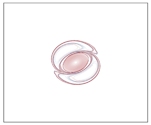
Figure 2. (a,b) Horizontal mid-plane cross-section of the PV jumps discretizing the PV field at  $t=9.55$ and $15.92$ for the CASL simulation. Red contours correspond to positive PV jumps, blue ones to negative PV jumps. (c) Orthographic view on the PV jumps at the edge of the vortex at $t=15.92$ (corresponding to the outermost PV jumps of figure 2). The vortex is viewed at an angle of $60^\circ$ from the vertical direction. The colour shading indicates the height of the PV jump (the top of the vortex is in light blue, the bottom of the vortex is in dark blue).

Figure 3. Horizontal, mid-plane cross-section of the PV field for the pseudo-spectral simulation of the perturbed 3-D MEV at (a)  $t=0,\ (\textit {b})$ $t=10$ ${\rm and}\ (\textit {c})$ t $=$
$=$  $19$.
$19$.
5. Conclusion
The mathematical calculation (with a variational method) determined that 3-D, minimal enstrophy, spherical vortices have opposite-signed QG potential vorticity radially. The internal potential vorticity distribution is continuous with that of the external fluid, which vanishes. Similarly, the rotational (azimuthal) velocity of the vortex increases quasi-linearly for a fifth of its total radius (or half of the maximum velocity radius), followed by a smoothly decaying tail. This is similar to the MEV M in 2-D incompressible fluids (Leith Reference Leith1984b). This is also in qualitative agreement with detailed measurements of deep vortices at sea (Paillet et al. Reference Paillet, Le Cann, Serpette, Morel and Carton1999, Reference Paillet, Cann, Carton, Morel and Serpette2002; Ayouche et al. Reference Ayouche, De Marez, Morvan, L'hegaret, Carton, Le Vu and Stegner2021). Recent results of very-high-resolution numerical simulations of the Atlantic Ocean (Chouksey Reference Chouksey2023), indicate that deep/bottom vortices mostly have a shield in potential vorticity. Note that our solutions (in spherical Bessel functions) bear similarity with those recently derived by Zoeller & Viudez (Reference Zoeller and Viudez2023), but from a different point of view (that of 3-D isotropic isolated vortices without the minimal-enstrophy constraint). Finally, it will be of interest to compare this MEV to 3-D maximum-entropy vortices, to be determined in the spirit of the work by Brands et al. (Reference Brands, Chavanis, Pasmanter and Sommeria1999), Fine et al. (Reference Fine, Cass, Flynn and Driscoll1995). Further work will be needed to
(i) assess analytically if non-axisymmetric 3-D MEVs can be determined analytically (and then compared with the end states of our numerical solutions),
(ii) extend the present work to non-geostrophic dynamics (rotating shallow-water model) and if possible, to 3-D continuously stratified flows.
Declaration of interests
The authors report no conflict of interest.
Appendix A. Variation according to the vortex radius $R$

Following Leith (Reference Leith1984b), we could have performed variations of the functional  $F(\psi )$ with respect to the vortex radius $R$, but this would have led to a relation between the Lagrange multipliers, and the enstrophy that we minimize (which is therefore unknown). Indeed, with dimensions, the variations of enstrophy $\delta _RZ$, energy $\delta _R E$ and angular momentum $\delta _RL$ are
 \begin{equation} \left. \begin{array}{@{}c@{}} \delta_R Z ={-}\dfrac{Z}{R} \delta R, \\ \delta_R E = \dfrac{E}{R} \delta R, \\ \delta_R L = \dfrac{4L}{R} \delta R. \end{array}\right\} \end{equation}
Minimizing variations leads to
 \begin{equation} Z ={-}\lambda E - 4 \mu L. \end{equation}
Therefore, the enstrophy would have been fixed by the energy and the generalized momentum provided, which would have led to a contradiction. In the 2-D case, the variation according to  $R$ does not involve the enstrophy and helps to find a relation between the energy and the angular momentum. Contrary to the 2-D case, the enstrophy is computed using the whole potential vorticity $q$ and thus the spherical Laplacian instead of the vertical vorticity $(\partial _x^2+\partial _y^2)\psi$ which gives a cylindrical Laplacian. Using the 2-D introduced radius $\rho$ and a cylindrical frame of reference would have led to a similar development as that of Leith (1984). The 3-D geometry makes this parameter inconsistent.


 Open access