


1. Introduction
Pressure-driven flow in ducts is a subject of utmost relevance in mechanical and aerospace engineering applications. In fact, effective design of ducts in cooling systems of liquid rocket engines is extremely important because of the harsh environment to which the system is subjected. The present authors (Nasuti, Torricelli & Pirozzoli Reference Nasuti, Torricelli and Pirozzoli2021) have recently carried out a numerical study of flow in smooth rectangular cooling ducts, and they found that traditional approaches such as Reynolds-averaged Navier–Stokes (RANS) can yield good prediction of the pressure drop. Most studies in ducts have been carried out for the canonical case of circular pipes with smooth walls, which has for instance been the focus of recent numerical studies at high Reynolds number (Pirozzoli et al. Reference Pirozzoli, Romero, Fatica, Verzicco and Orlandi2021). The case of rough walls is however at least as important, but so far it has mainly received attention through experimental studies. Recent technological advances in the field of additive manufacturing have further prompted investigations of flow over surfaces with larger relative roughness than the one studied so far (Calignano et al. Reference Calignano, Manfredi, Ambrosio, Iuliano and Fino2013; Snyder et al. Reference Snyder, Stimpson, Thole and Mongillo2016; Stimpson et al. Reference Stimpson, Snyder, Thole and Mongillo2016). Additive manufacturing indeed allows one to build three-dimensional objects starting from a digitised three-dimensional model and adding material such as plastics, liquids or powder grains being fused, typically layer by layer. This procedure allows for instance machine cooling channels with more complex geometry and smaller size, however it also yields large relative roughness, which can affect frictional drag significantly. Understanding the behaviour of flows over irregular rough surfaces with higher relative roughness than studied in most experiments is thus certainly of great practical interest.
The systematic experimental investigation carried out by Nikuradse (Reference Nikuradse1933) is widely regarded as the starting point for the study of turbulent flows over rough walls. Nikuradse compiled an extensive database for fully developed flow in circular pipes whose walls were covered with unstructured roughness consisting of sieved sand grains, and found non-monotonic behaviour of the friction factor with change of the Reynolds number. He also noticed that for all the tested surfaces the transition from laminar to turbulent flow occurred roughly at the same critical Reynolds number ( $Re_b \approx 2000$). Last, he noticed that in the fully turbulent regime the larger the roughness the higher is the friction factor, whereas in the laminar regime the friction factor of all the tested rough surfaces collapsed to the smooth pipe case. Since reproduction of the exact kind of surface used in Nikuradse's experiments is almost impossible, no later studies succeeded in precisely reproducing his results. Later research on the subject was carried out by Colebrook et al. (Reference Colebrook, Blench, Chatley, Essex, Finniecome, Lacey, Williamson and Macdonald1939), who investigated flow in commercial galvanised, cast- and wrought-iron pipes, for which the friction factor displayed monotonic decrease with the Reynolds number in the transitionally rough regime. It was generally believed that the different behaviour observed in Nikuradse's and Colebrook's experiments is due to the presence of roughness elements of one size in the former case, whereas it is expected that realistic engineering surfaces which feature roughness elements with disparate sizes should more closely follow Colebrook's trends. However, some recent experimental studies refuted this assumption, showing that a wide range of irregular surfaces more closely follow Nikuradse's behaviour instead of Colebrook's. It is the case for surfaces finished with a honing tool (Schultz & Flack Reference Schultz and Flack2007), sanded surfaces (Flack, Schultz & Rose Reference Flack, Schultz and Rose2012), grit-blasted surfaces (Flack et al. Reference Flack, Schultz, Barros and Kim2016) and sandpaper (Flack & Schultz Reference Flack and Schultz2023).
Experimental investigations over rough surfaces have mainly been carried out inside plane channels. The only available experimental results concerning pipes with very large relative roughness are due to Huang et al. (Reference Huang, Wan, Chen, Li, Mao and Zhang2013). Those authors studied both the laminar and the turbulent regime and found that the friction factor behaves differently than found by Nikuradse, for high relative roughness. In particular, the transition from the laminar to the turbulent regime was found to occur at bulk Reynolds number less than 2000. Moreover, Huang et al. (Reference Huang, Wan, Chen, Li, Mao and Zhang2013) found that in the laminar region the larger the roughness, the higher the friction factors, with deviations from the analytical friction formula for the smooth pipe.
Most studies published to date aim at evaluating an equivalent sand-grain roughness height ( $k_s$), for rough surfaces with different geometries. The equivalent sand-grain roughness, first defined by Schlichting (Reference Schlichting1936), is the size of sand grains in Nikuradse's experiments which yield the same drag as the surface under consideration. The behaviour of rough walls is primarily controlled by the parameter $k_s^+ = k_s / \delta _v$ (where $\delta _v=\nu /u_{\tau }$, and $u_{\tau }=(\tau _w/\rho )^{1/2}$ are the viscous length scale and the friction velocity), namely the ratio of the equivalent sand-grain roughness height to the viscous length scale. Based on the value of $k_s^+$, Nikuradse (Reference Nikuradse1933) identified three flow regimes: hydraulically smooth, transitionally rough and fully rough. In the first regime the height of the roughness is of the order of the viscous sublayer, hence roughness does not affect the flow behaviour. In the transitionally rough regime, the behaviour of the flow instead depends strongly on the geometrical parameters of the roughness. Finally, in the fully rough regime the friction coefficient is nearly unaffected by Reynolds number variations.
The presence of roughness affects both the mean flow and the turbulent motion of a fluid, which entails an increase of friction with respect to the smooth wall case. This is linked to the downward shift in the inner-scaled profile of the mean streamwise velocity, which can be expressed through the roughness function (Clauser Reference Clauser1954; Hama Reference Hama1954),
 \begin{equation} \Delta U^+ = \frac{1}{\kappa} \log k^+ + A - B(k^+) , \end{equation}
where  $\kappa (\approx 0.4)$ is the von Kármán constant, $A (\approx 5.0)$ is the log-law intercept for flow over smooth walls, and $B$ is a function of both the roughness topography and the roughness Reynolds number $k^+$. The hydraulically smooth regime is realised for small $k^+$ ( $\Delta U^+ \approx 0$). As $k^+$ increases the roughness function becomes non-zero, and the flow is transitionally rough. In this regime the shape of $\Delta U^+$ in the Nikuradse-type roughness exhibits an inflectional behaviour, whereas it is more gradual in Colebrook-type roughness. The fully rough regime is achieved for $\Delta U^+ > 7$, in which case $B$ becomes independent of $k^+$, while still depending on the roughness geometry. Hence, the equivalent roughness height can be estimated for any kind of rough surface by making the roughness function collapse to Nikuradse's results in this universal regime. For the so-called $k$-type roughness (Jiménez Reference Jiménez2004), $k_s$ is proportional to $k$, and their ratio is referred to as the reduction coefficient (Schlichting Reference Schlichting1936).
So far, past studies focused on the demonstration of the validity of Townsend's outer-layer similarity hypothesis (Townsend Reference Townsend1976). According to that hypothesis, smooth and rough wall turbulence behave similarly away from the wall at sufficiently high Reynolds number in the presence of sufficient scale separation between the typical roughness height ( $k$) and the outer length scale of the flow ( $\delta$, e.g. the pipe diameter). Jiménez (Reference Jiménez2004) stated that scale separation requires $k/\delta \lesssim 1/40$. However, several studies have shown that outer-layer similarity still holds in the wake region of the wall layer for surfaces with higher relative roughness (Chan et al. Reference Chan, MacDonald, Chung, Hutchins and Ooi2015; Busse, Thakkar & Sandham Reference Busse, Thakkar and Sandham2017; Forooghi et al. Reference Forooghi, Stroh, Magagnato, Jakirlić and Frohnapfel2017). Jiménez (Reference Jiménez2004) defined this kind of roughness as ‘obstacles’, and stated that its behaviour is highly dependent on its geometry.
So far, direct numerical simulations (DNS) have been mainly focused on structured roughness. Leonardi et al. (Reference Leonardi, Orlandi, Djenidi and Antonia2004) studied the organised motion in a turbulent channel flow with transversal square bars, and Orlandi, Leonardi & Antonia (Reference Orlandi, Leonardi and Antonia2006) focused on channel flows with two-dimensional roughness elements of various shapes. They noticed that the wall-normal and spanwise velocity fluctuations increase with respect to the smooth wall case, whereas the streamwise velocity fluctuations do not, suggesting that isotropy is more closely achieved over a rough wall than over a smooth wall. Only Chan et al. (Reference Chan, MacDonald, Chung, Hutchins and Ooi2015) has carried out DNS in a rough pipe, albeit with a specific focus on deterministic, sinusoidal roughness. Those authors found that Townsend's outer-layer similarity was achieved with universality of the first- and second-order statistics, provided  $k/\delta \lesssim 1/7$, hence much higher value than proposed by Jiménez (Reference Jiménez2004).
DNS studies of turbulent flow over irregular roughness have also been recently carried out, limited to the case of flow in plane channels. In a series of studies, Busse et al. (Reference Busse, Thakkar and Sandham2017) and Thakkar, Busse & Sandham (Reference Thakkar, Busse and Sandham2017, Reference Thakkar, Busse and Sandham2018) investigated the flow over many kinds of rough surfaces that were scanned and suitably filtered. Also in this case the behaviour of the friction coefficient was found to be similar to that proposed by Nikuradse. In particular, the roughness function for the grit-blasted surface studied in Thakkar et al. (Reference Thakkar, Busse and Sandham2018) was found to closely follow Nikuradse's results, hence this kind of roughness can be regarded as a digital representation or surrogate for Nikuradse's sand-grain roughness. At the highest Reynolds numbers under consideration ( $Re_b \approx 16\,000$), those authors confirmed that Townsend's outer layer similarity was verified, provided $k/\delta \approx 1/6$. Many previous studies have attempted to determine a priori correlations between $k_s$ and the geometrical parameters of the roughness. These correlations have been explored in both experimental (Flack & Schultz Reference Flack and Schultz2010; Flack et al. Reference Flack, Schultz, Barros and Kim2016; Flack, Schultz & Barros Reference Flack, Schultz and Barros2020) and numerical research (Chan et al. Reference Chan, MacDonald, Chung, Hutchins and Ooi2015; Forooghi et al. Reference Forooghi, Stroh, Magagnato, Jakirlić and Frohnapfel2017; De Marchis et al. Reference De Marchis, Saccone, Milici and Napoli2020). In a recent study, Jouybari et al. (Reference Jouybari, Yuan, Brereton and Murillo2021) introduced a novel approach by employing deep neural network (DNN) and Gaussian process regression (GPR) techniques.
A comprehensive overview of studies of flow over rough walls has recently been compiled by Chung et al. (Reference Chung, Hutchins, Schultz and Flack2021). One of the conclusions of that study is however that ‘Effort is required for predicting heat and mass transfer [ $\cdots$] and improving our understanding of the influence of topography’. The present work aims at investigating the influence of relatively large roughness on the flow inside circular pipes, with the goal of characterising the flow structure and trying to characterise the equivalent sand-grain roughness, for the case of a grit-blasted surface and a graphite-like surface. A relatively wide range of Reynolds numbers is investigated, up to the fully rough regime, to allow direct comparison with Nikuradse's friction diagram.
2. Methodology
2.1. Numerical method and definitions
A second-order finite-difference discretisation of the incompressible Navier–Stokes equations in Cartesian coordinates is used, based on the classical marker-and-cell method (Harlow & Welch Reference Harlow and Welch1965; Orlandi Reference Orlandi2000), with staggered arrangement of the flow variables to remove odd–even decoupling phenomena and guarantee discrete conservation of the total kinetic energy in the inviscid flow limit. Uniform volumetric forcing is applied to the streamwise momentum equation through a time-varying pressure gradient  $\varPi$, to maintain constant mass flow rate in time. The Poisson equation resulting from enforcement of the divergence-free condition is efficiently solved by double trigonometric expansion in the streamwise and spanwise directions, and inversion of tridiagonal matrices in the third direction (Kim & Moin Reference Kim and Moin1985). An extensive series of previous studies about wall-bounded flows from this group proved that second-order finite-difference discretisation yields in practical cases of wall-bounded turbulence results which are by no means inferior in quality to those of pseudospectral methods (e.g. Pirozzoli, Bernardini & Orlandi Reference Pirozzoli, Bernardini and Orlandi2016). A hybrid third-order Runge–Kutta algorithm is used for time integration, whereby the convective terms are treated explicitly, and the diffusive terms are handled implicitly to alleviate the time step limitation.
The computational domain is a rectangular box of size  $L_x \times L_y \times L_z$, covered with a uniform Cartesian mesh, as shown in figure 1 for a representative pipe cross section. A rough pipe with mean radius $R$ and cross-sectional area $A={\rm \pi} R^2$ is embedded in it, and the no-slip boundary conditions are approximately enforced through the immersed-boundary method. As a preliminary step, the pipe geometry is generated in the standard Stereo-LiThography format, and a geometrical preprocessor based on the ray-tracing algorithm (O'Rourke et al. Reference O'Rourke1998) is applied to discriminate grid points belonging to the fluid and the solid phase (Iaccarino & Verzicco Reference Iaccarino and Verzicco2003). Near the fluid–solid interface the viscous terms dominate the nonlinear and pressure terms, hence the boundary conditions can be enforced by locally changing the finite-difference weights for the approximation of the second derivatives (Orlandi & Leonardi Reference Orlandi and Leonardi2006). The predictive capability of the method for the numerical simulation of turbulent flows over rough surfaces was documented in a large number of papers (e.g. Iaccarino & Verzicco Reference Iaccarino and Verzicco2003; Nikitin & Yakhot Reference Nikitin and Yakhot2005; Orlandi & Leonardi Reference Orlandi and Leonardi2006; Burattini et al. Reference Burattini, Leonardi, Orlandi and Antonia2008; Bernardini, Modesti & Pirozzoli Reference Bernardini, Modesti and Pirozzoli2016; Orlandi, Modesti & Pirozzoli Reference Orlandi, Modesti and Pirozzoli2018).

Figure 1. Schematic representation of the grid of a pipe cross section. Black solid lines represent the rough surface boundary, red dashed lines indicates the mean pipe surface.
The controlling parameter of the flow is the bulk Reynolds number  $Re_b = 2 R u_b / \nu$, where
 \begin{equation} \quad u_b = \frac 1V \int_{V} U \, {\rm d} V , \end{equation}
is the bulk velocity, with  $U$ the mean streamwise velocity and $V$ the fluid volume. The resulting friction Reynolds number is $Re_{\tau } = R u_{\tau } / \nu$, where the friction velocity is evaluated based on the measured pressure gradient, $\tau _w = R/2 \langle \varPi \rangle$. Hereafter, uppercase letters are used to denote flow properties averaged in the streamwise direction and in time, lowercase letters denote fluctuations thereof and brackets denote the averaging operator. The $+$ superscript is here used to denote wall units, namely quantities made non-dimensional with respect to the friction velocity and the viscous length scale.
2.2. Roughness geometry
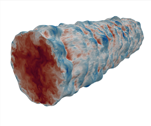
Two types of rough surfaces are considered, both taken from the University of Southampton Institutional Repository (Thakkar, Busse & Sandham Reference Thakkar, Busse and Sandham2016). The first, shown in figure 2(a), derives from the scan of a grit-blasted surface, and the second, shown in figure 2(b), derives from a sample of graphite. In both cases a low-pass Fourier filter was applied to the scanned roughness profiles. This post-processing procedure is necessary as surface scans generate noise which needs to be removed, and because a smoothly varying periodic surface is required to impose periodic numerical boundary conditions in the streamwise direction. Full information about the database is available in Thakkar et al. (Reference Thakkar, Busse and Sandham2017). The rough pipe geometries shown in panels (c) and (d) were then obtained by doubling the baseline samples in the spanwise direction, and wrapping the surfaces thus obtained around the mean pipe geometry. This procedure guarantees preservation of geometrical similarity of the roughness, while modifying the relative roughness height, which is  $1/6$ of the channel half-height for Thakkar et al. (Reference Thakkar, Busse and Sandham2017), and $k/R \approx 1/5$ in our case.

Figure 2. Topography of rough surfaces. Panels (a) and (b) show the geometries of grit-blasted surface and graphite surface, originally used for channel flow (Thakkar et al. Reference Thakkar, Busse and Sandham2017), with the colour map showing the elevation normalised by the channel half-height. Panels (c) and (d) show the geometries obtained by wrapping the original rough surfaces around the pipe as explained in the text.
Table 1 displays some relevant geometrical parameters which characterise the resulting roughness. In this study we define the roughness height to be the mean-peak-to-trough height ( $k$), as obtained by partitioning the surface into $5 \times 5$ tiles of equal size and then computing the average of the difference between the maximum and minimum height for each tile (Thakkar et al. Reference Thakkar, Busse and Sandham2017). Other parameters commonly used to quantify roughness are the average roughness height,
 \begin{equation} S_a=\sum_{i,j}^{M,N} |h_{i,j}| / ( M N) , \end{equation}
and the root-mean-square roughness height,
 \begin{equation} S_q=\sqrt{\sum_{i,j}^{M,N} h_{i,j}^2} / (M N) , \end{equation}
where  $h_{i,j}$ are roughness heights obtained after the filtering procedure, and $M$ and $N$ are the number of data points in the streamwise and spanwise directions. Other relevant parameters include the skewness,
 \begin{equation} {Sk}=\sum_{i,j}^{M,N} h_{i,j}^3/ (M N S_q^{3}) , \end{equation}
and the maximum peak-to-trough height,
 \begin{equation} S_{z,{z,max}}=max(h_{i,j})- min(h_{i,j}) . \end{equation}
The last parameter reported in table 1 is the effective slope, defined as
 \begin{equation} ES=\frac{1}{L_xL_y}\int_{0}^{L_x}\int_{0}^{L_y} \left| \frac{{\rm d} h}{{\rm d}\kern 0.06em x} \right|_{i,j} \, \text{d}\kern 0.06em x\,\text{d}y, \end{equation}
where  $L_x$ and $L_y$ are the dimensions of the baseline smooth surface along the streamwise and spanwise directions.
Table 1. Geometrical properties of the rough pipe surfaces considered in this study.

The pipe length is about  $L_x = 6.27 R$, in both cases. The computational domain in the cross-stream directions measures $L_y = L_z = 2.45 R$, for the grit-blasted surface, and $L_y = L_z = 2.29 R$, for the graphite surface, such that the roughness is wholly confined. Preliminary studies have been carried out to establish the sensitivity of the computed results on the length of the pipe. DNS in axially doubled domains have in fact shown that, for given grid resolution, the friction factor $f = 8 \tau _w /(\rho u_b^2)$ (and other key statistics) varies by no more than $1$ %. Hence, the baseline domain only is considered from now on. It is also important to note that in the forthcoming presentation of the results, the wall distance $y$ is measured from the roughness centroid, hence negative $y$ are allowed. We set $y=0$ corresponding to the mean pipe radius, in such a way to achieve collapse of the total stress to the smooth-wall case (Chan et al. Reference Chan, MacDonald, Chung, Hutchins and Ooi2015; Thakkar Reference Thakkar2017), as shown in § 3.2. Although alternative definitions of the virtual origin are possible, for instance in terms of the height of the roughness at which the integrated resultant force acts (Chan et al. Reference Chan, MacDonald, Chung, Hutchins and Ooi2015), that is impossible to implement within the immersed-boundary approach which we use.
Establishing the appropriate grid resolution in numerical simulations of turbulence over rough wall is a very important and tricky subject, as discussed by Busse, Lützner & Sandham (Reference Busse, Lützner and Sandham2015). In particular, those authors noticed that at least 12 grid points per roughness feature should be used for accurate characterisation of roughness effects. In order to address this issue, we have carried out a grid sensitivity analysis at  $Re_b = 4400$, for both roughness geometries, which has shown that at least $N_x=384$ grid points should be used along the streamwise direction, and $N_y=N_z=192$ grid points should be used in the transversal directions, which would correspond to about 15 grid points per roughness element, thus corroborating the findings of Busse et al. (Reference Busse, Lützner and Sandham2015). The results of the grid sensitivity analysis for the grit-blasted surface are shown in the Appendix.
DNS for the two rough pipe geometries have been carried out for a wide range of Reynolds numbers, from  $Re_b = 500$ to $Re_b = 30\,000$, with test conditions listed in table 2. The number of grid points has been progressively increased with the Reynolds number. A grid sensitivity analysis has been carried out also for the graphite surface at $Re_b = 30\,000$ (in which a fully rough regime is established), to verify that the uncertainty in the key parameters ( $\,f, k^+$) is acceptable. The time step expressed in wall units ( $\nu /u_\tau ^2$) ranges from about $\Delta t^+=0.015$ for the cases at $Re_b = 500$ to about $\Delta t^+=0.29$ for the cases at $Re_b = 30\,000$. The time intervals used to collect the flow statistics are also reported in table 2 in terms of eddy-turnover times ( $\tau _t=R/u_\tau$), are typically much longer than the current practice in DNS of smooth channels and pipes (Hoyas & Jimenez Reference Hoyas and Jimenez2006; Pirozzoli et al. Reference Pirozzoli, Romero, Fatica, Verzicco and Orlandi2021), for the sake of achieving convergence of the statistical properties in the cross-stream plane.
Table 2. Flow parameters for flow in pipes with rough walls. The first set of parameters pertains to the grit-blasted surface. In these cases the computational box dimensions are  $6.28 R \times 2.45 R \times 2.45 R$. The second set of parameters pertains to the graphite surface, and the box dimensions are $6.27 R \times 2.29 R \times 2.29 R$. Here $Re_b = 2 R u_b / \nu$ is the Reynolds number, $Re_{\tau } = R u_{\tau } / \nu$ is the friction Reynolds number, $k^+=k u_{\tau }/\nu$ is the roughness Reynolds number, $f = 8 \tau _w /(\rho u_b^2)$ is the friction factor and $N_x$, $N_y$ and $N_z$ denote the number of grid points in the streamwise, and the two cross-stream directions. Finally, $\Delta x^+$, $\Delta y^+$ and $\Delta z^+$ are the grid spacings in the streamwise and cross-stream directions, given in wall units, $T$ is the time interval used to collect the flow statistics and $\tau _t=R/u_\tau$ is the eddy turnover time.

2.3. Validation
Preliminary validation of the code was carried out by simulating the flow inside a smooth pipe at  $Re_b=5300$. The results have been compared with those obtained by Pirozzoli et al. (Reference Pirozzoli, Romero, Fatica, Verzicco and Orlandi2021), using a body-fitted solver for cylindrical coordinates. Figure 3 depicts the profiles of the streamwise velocity and of the velocity variances and turbulent shear stress. The results are quite satisfactory, as the computed $Re_{\tau }$ differ by less than $1\,\%$, and the profiles of the statistical quantities are in very good agreement.

Figure 3. DNS of flow in a smooth pipe: (a) mean streamwise velocity  ${U}^+$; (b) velocity variances $\langle u_x^2 \rangle$ ( $\lozenge$), $\langle u_r^2 \rangle$ ( $\square$), $\langle u_{\varTheta }^2 \rangle$ ( $\triangle$) and the average of fluctuations product $\langle u_x u_r \rangle$ ( $\nabla$). Filled symbols denote results of the present DNS and open symbols denote those obtained by Pirozzoli et al. (Reference Pirozzoli, Romero, Fatica, Verzicco and Orlandi2021). The directory including the data and the Jupyter notebook can be accessed at https://www.cambridge.org/S0022112023007280/JFM-Notebook/files/Figure-3/velocity_validation_smooth.ipynb.
Additional validation included reproducing some DNS results for flow in a plane channel (Busse et al. Reference Busse, Thakkar and Sandham2017; Thakkar et al. Reference Thakkar, Busse and Sandham2018). Two Reynolds numbers ( $Re_\tau = 180$ and $360$) have been considered for each type of roughness, and the key results are presented in table 3. Figure 4 also compares profiles of the mean streamwise velocity, and the roughness function as a function of the roughness Reynolds number. In this respect we must specify that we have re-evaluated the data of Busse et al. (Reference Busse, Thakkar and Sandham2017), since we define the roughness function based on the difference of the velocity profiles within the overlap layer Hama (Reference Hama1954), whereas those authors considered the difference of the centreline values. The results are in general good agreement, difference of the computed $Re_{\tau }$ being no larger than $2$ %. This discrepancy is however noticeable in the diagram of the roughness function. A thorough grid sensitivity study has thus been carried out, which has shown no hint of lack of sufficient resolution, hence we believe that remaining differences could be due to different implementation of the immersed-boundary technique.
Table 3. Results of the validation study for smooth and rough plane channels.


Figure 4. DNS of flow in rough channel: mean streamwise velocity  ${U}^+$ for grit-blasted (a) and graphite (b) (symbols as in table 3); (c) roughness function as a function of roughness Reynolds number (symbols as in table 3). The directory including the data of the profiles and the Jupyter notebook can be accessed at https://www.cambridge.org/S0022112023007280/JFM-Notebook/files/Figure-4a-b/channel_validation.ipynb. The roughness functions and the Jupyter notebook can be accessed at https://www.cambridge.org/S0022112023007280/JFM-Notebook/files/Figure-4c/deltau.ipynb.
3. Results for rough pipes
The key one-point flow statistics are hereafter reported, as obtained by averaging in time and in the streamwise direction, limited to the volume occupied by the fluid. Figure 5 depicts the mean streamwise velocity distribution over the cross section of the pipe, also within the roughness. Owing to the large relative roughness, the fields do not show any symmetry, thus confirming that for  $R/k \lesssim 40$ the effect of the wall is felt throughout the wall layer (Jiménez Reference Jiménez2004). Furthermore, according to Chung et al. (Reference Chung, Hutchins, Schultz and Flack2021) and Jelly et al. (Reference Jelly, Ramani, Nugroho, Hutchins and Busse2022), the diameter and the strength of the secondary flows is sensitive to the spanwise length scale of the roughness in proportion to the outer scale of the problem, say $\delta$. Specifically, Chung et al. (Reference Chung, Hutchins, Schultz and Flack2021) state that the diameter of the secondary flows is about $\delta$ when the spanwise wavelength of the roughness matches or exceeds the outer scale, here the pipe radius. In the present study, the longest azimuthal wavelength is half the circumference of the pipe. Consequently, the lack of axisymmetry in the velocity field even far from the wall might just as well be due to the large azimuthal length scale, which yields a large secondary flow. Furthermore, the velocity isolines show clear sensitivity to Reynolds number variations and to the roughness geometry.

Figure 5. Contours of mean streamwise velocity for the grid-blasted surface (a–c) and the graphite surface (d–f), with symbols referring to the flow conditions in table 2: (a)  $\bullet$ orange; (b) $\bullet$ green; (c) $\bullet$ blue; (d) $\circ$ orange; (e) $\circ$ green; and ( f) $\circ$ blue. The dashed line marks the mean pipe surface and the solid line marks the plane of the crests. The boundary of the maps corresponds to points beyond which no fluid element if found.
Figure 6 depicts the wall-normal profiles of the streamwise velocity, obtained by further averaging in the azimuthal direction. The figure shows that increase of  $k^+$ yields a downward shift of the velocity profiles with respect to the case of a smooth pipe, thus yielding a larger roughness function. Near the wall, the behaviour is the opposite, as DNS at higher $k^+$ have higher mean velocity, since the flow is capable of penetrating deeper into the roughness canopy (Busse et al. Reference Busse, Thakkar and Sandham2017; Thakkar et al. Reference Thakkar, Busse and Sandham2018). Despite the high relative roughness, a logarithmic layer can still be identified in all cases, with slope similar to the smooth wall case, which allows us to consistently define a roughness function.

Figure 6. Profiles of streamwise velocity for the grit-blasted surface (a) and the graphite surface (b) at various Reynolds numbers, symbols as in table 2. The black line corresponds to the smooth wall case. The directory including the data of the profiles and the Jupyter notebook can be accessed at https://www.cambridge.org/S0022112023007280/JFM-Notebook/files/Figure-6/velocity.ipynb.
Figure 7 shows the same velocity profiles in defect form. Some scatter is, in fact, observed away from walls (say,  $y/R \gtrsim 0.2$), for both roughness geometries, which however tends to be reduced as $Re$ grows. In particular, the grit-blasted surface seems to exhibit collapse to the smooth wall velocity profile once a fully rough regime is attained, with $4\,\%$ deviations at most, at $Re_b=30\,000$. Poorer collapse observed in the case of the graphite surface could be due to higher relative roughness, In that case, deviation are $13\,\%$ at most, at $Re_b=30\,000$. Validity of Townsend's outer-layer similarity for the velocity profile over structured and unstructured rough surfaces was previously documented by Orlandi & Leonardi (Reference Orlandi and Leonardi2006), Busse et al. (Reference Busse, Thakkar and Sandham2017), Thakkar et al. (Reference Thakkar, Busse and Sandham2018), MacDonald, Hutchins & Chung (Reference MacDonald, Hutchins and Chung2019), Flack, Schultz & Shapiro (Reference Flack, Schultz and Shapiro2005) and Jiménez (Reference Jiménez2004). Despite large relative roughness, our DNS provides evidence that close similarity is achieved even at $k / R \approx 1/5$. Given the severe non-uniformities observed in figure 5, the fact that the azimuthally averaged velocity profiles still bear close resemblance to those found in the case of smooth walls further points to the importance of the imposed spatially uniform pressure gradient, rather than the local wall conditions. Similar observations were reported by Pirozzoli et al. (Reference Pirozzoli, Modesti, Orlandi and Grasso2018) for flow in smooth square ducts.

Figure 7. Velocity defect profiles ( $U_c^+-U^+$, with $U_c$ the mean centreline velocity) for the grit-blasted surface (a) and the graphite surface (b) at various Reynolds numbers, with symbols defined in table 2. The black line corresponds to the smooth wall case. The vertical solid line corresponds to the plane of the crests and the dashed line marks the roughness centroid $y/R=0$. The directory including the data of the profiles and the Jupyter notebook can be accessed at https://www.cambridge.org/S0022112023007280/JFM-Notebook/files/Figure-7/velocity_defect.ipynb.
3.1. Friction
In figure 8 the friction factors obtained from the present DNS are superposed to Nikuradse's chart, with the obvious caveat that the relative roughness in those experiments is much less than in our case. Referring to the laminar flow region in the low- $Re$ end of the graph, in Nikuradse's experiments the friction factor for all surfaces collapsed to the Hagen–Poiseuille prediction $f=64/Re_b$, thus suggesting that friction is not affected by the change of the wall geometry. In the present DNS we find instead that the computed friction factors are higher than the expected theoretical values by about 5–9 %. This indicates that in our case the larger relative roughness has the role of altering the geometry of the pipe, thus producing modification also in the laminar flow regime. Similar findings where reported by Huang et al. (Reference Huang, Wan, Chen, Li, Mao and Zhang2013), who found that deviations from the viscous theory appears for relative roughness of about $14\,\%$. In that study, Huang et al. (Reference Huang, Wan, Chen, Li, Mao and Zhang2013) carried out the experiments by considering a pipe with wall covered with spheres of various diameter to simulate roughness with different height. In that case, the relative roughness height was defined as the ratio between the diameter of the spheres and the radius of the pipe without the spheres.

Figure 8. (a) Variation of friction factor ( $\,f$) with bulk Reynolds number ( $Re_b$) based on the mean radius ( $R$). (b) Variation of friction factor with the effective bulk Reynolds number ( $Re_{h}$) based on the effective radius ( $R_{h}$). Nikuradse's data are shown for pipes with various relative roughness height ( $k/R$). The dashed line denotes the Hagen–Poiseuille $f=64/Re_b$ friction law and the solid line denotes the Prandtl friction law for turbulent pipe flow. The directory including the data and the Jupyter notebook can be accessed at https://www.cambridge.org/S0022112023007280/JFM-Notebook/files/Figure-8/Nikuradse.ipynb.
The large relative roughness in the pipe geometries under consideration has the intuitive effect of reducing the available pipe area for fluid flow, thus the effective radius of the pipe is smaller than the geometrical mean radius. Kandlikar et al. (Reference Kandlikar, Schmitt, Carrano and Taylor2005) defined the effective radius of the pipe by subtracting the average roughness height from the mean radius, however in that case the effective radius would change according to the definition of the average roughness height, which is not universal. In the present study, we define the effective radius to be the hydraulic radius, which is traditionally used for friction prediction in non-circular ducts, and defined as  $R_{h}=2 {V}/{S}$, where $V$ is the volume occupied by the fluid and $S$ is the area of the wetted surface. Figure 8(b) shows the Nikuradse diagram obtained by replacing $Re_b$ with $Re_{h}= 2 R_h u_b / \nu$. In this representation we find that the results collapse to the Hagen–Poiseuille prediction to within less than $1\,\%$.
Huang et al. (Reference Huang, Wan, Chen, Li, Mao and Zhang2013) also noticed that the larger the relative roughness, the lower the Reynolds number at which transition from laminar to turbulent regime occurs. This prediction is corroborated by the present data, and in fact transition occurs earlier for the graphite surface than the grit-blasted surface, on account of higher relative roughness. Transition is found to occur similarly (but perhaps more sharply) than in Nikuradse's experiments. Most interestingly, the friction factor past the transition point is found to increase with the Reynolds number, consistent with numerical simulations in channels with the same roughness geometry (Busse et al. Reference Busse, Thakkar and Sandham2017). However, the behaviour in this regime is known to be significantly affected by the nature of the roughness (Colebrook et al. Reference Colebrook, Blench, Chatley, Essex, Finniecome, Lacey, Williamson and Macdonald1939; Jiménez Reference Jiménez2004; Flack et al. Reference Flack, Schultz and Rose2012, Reference Flack, Schultz and Barros2020). Evidence for the establishment of a fully rough regime is found at the highest Reynolds numbers considered, which show very small variation of the friction factor (also see table 2).
In figure 9(a) we show the roughness function for our DNS (determined based on the log-law shift) as a function of  $k^+$. In the figure we also show data from the channel flow DNS of Busse et al. (Reference Busse, Thakkar and Sandham2017), from Nikuradse's experiment (Nikuradse Reference Nikuradse1926) and Colebrook's relation (Colebrook et al. Reference Colebrook, Blench, Chatley, Essex, Finniecome, Lacey, Williamson and Macdonald1939)
 \begin{equation} \Delta U^+ = 1/\kappa \log ( 1+0.3 k^+ ) . \end{equation}
The procedure which we use to determine the roughness function relies on comparing the mean velocity profiles for a rough pipe with the mean velocity profile for a smooth pipe at the same (or similar)  $Re_{\tau }$, using the database of Pirozzoli et al. (Reference Pirozzoli, Romero, Fatica, Verzicco and Orlandi2021). We visually identify a log layer, and then determine the additive constant by fitting the data with a logarithmic function with prefactor $1/\kappa$, following the approach of Orlandi & Leonardi (Reference Orlandi and Leonardi2006), and as illustrated in figure 10.

Figure 9. Variation of roughness function with inner-scale roughness height (a) and with equivalent sand-grain roughness height (b). The dashed line denotes Colebrook's relation (Colebrook et al. Reference Colebrook, Blench, Chatley, Essex, Finniecome, Lacey, Williamson and Macdonald1939),  $\Delta U^+ = 1/\kappa \log ( 1+0.3 k_s^+ )$. The solid circles denote data from the present DNS: red, grit-blasted surface; blue, graphite surface. The open circles denote values taken from Nikuradse's experiment, and the triangles results of Busse et al. (Reference Busse, Thakkar and Sandham2017), for grit-blasted surface (red) and graphite surface (blue). The directory including the data of the profiles and the Jupyter notebook can be accessed at https://www.cambridge.org/S0022112023007280/JFM-Notebook/files/Figure-9.

Figure 10. Procedure for determination of the roughness function: mean streamwise velocity profiles for grit-blasted surface at  $Re_b=9800$ (green line), compared with smooth pipe at $Re_{\tau } = 495$ (black line). The dashed lines denote the functional relation $U^+=1/0.39 \log y^+ +A$, with $A=-2.86$ and $A=5$, respectively, as resulting from data fitting.
When reported as a function of  $k^+$, the roughness function has a trend quite similar to that observed in Nikuradse's experiments, and consistent with the channel flow DNS of Busse et al. (Reference Busse, Thakkar and Sandham2017), whereas data depart from Colebrook's relation at $k^+ \lesssim 50$. Consistent with observations made regarding the friction chart, we find that our data exceed $\Delta U^+ = 7$, which is the commonly accepted threshold for achievement of the fully rough regime. In the fully rough region, the difference of the roughness function in pipe and channel flow for given roughness is about $5\,\%$, which points to the non-negligible effect of the duct geometry in the presence of large roughness as in the present case. As is customary (Jiménez Reference Jiménez2004) we proceed to determine values of the equivalent sand-grain roughness height, by enforcing universality of the roughness function to the fully rough asymptote of (3.1). Data fitting of our DNS results yields $k_s^+ \approx 0.76 k^+$ for the grit-blasted surface, and $k_s^+ \approx 1.0 k^+$ for the graphite sample. Data fitting of the channel flow DNS results of Busse et al. (Reference Busse, Thakkar and Sandham2017) yields instead $k_s^+ \approx 0.68 k^+$ for the grit-blasted surface, and $k_s^+ \approx 0.83 k^+$ for the graphite sample. Once the roughness function is plotted against $k^+_s$, we note that the trend of $\Delta U^+$ collapses to Nikuradse's results throughout, which is an indication that both surfaces under consideration behave as Nikuradse's roughness. In order to analyze the behaviour at yet lower $k^+_s$, we should use a very low Reynolds number, given the large value of $k/R$ in our roughness. However at low $Re$ it is difficult to define a proper logarithmic region to consistently evaluate the roughness function. Another approach would be to consider lower $k/R$, which however would make the simulations computationally much more demanding.
3.2. Statistics of velocity fluctuations
In figure 11 we show the distribution of the velocity variances as a function of the outer-scaled wall distance. For reference, data for smooth pipes (Pirozzoli et al. Reference Pirozzoli, Romero, Fatica, Verzicco and Orlandi2021) are also shown at various  $Re_{\tau }$. Regarding the streamwise velocity variance, the structure is overall similar to the smooth wall case, with a near-wall peak associated with the presence of streaks. However, the amplitude of the peak is less than in the smooth case, for given $Re_{\tau }$, which is an indication that roughness tends to disrupt the classical near-wall cycle of turbulence regeneration (Orlandi et al. Reference Orlandi, Leonardi and Antonia2006), diverting kinetic energy from the streamwise direction to the other velocity components. We further find that as the Reynolds number increases, the near-wall peak is shifted outwards, suggesting that turbulent structures can penetrate deeper into the roughness canopy. On the other hand, the amplitude of the peak is barely affected, especially in the case of the graphite surface. This might point to modifications of outer-layer influences (Townsend Reference Townsend1976; Marusic, Baars & Hutchins Reference Marusic, Baars and Hutchins2017), or more probably to compensation between decrease resulting from higher $k^+$, and decrease due to logarithmic increase with $Re_{\tau }$ resulting from outer eddies. Our results also corroborate the findings of Busse & Sandham (Reference Busse and Sandham2012) and De Marchis, Napoli & Armenio (Reference De Marchis, Napoli and Armenio2010), who reported decrease of the streamwise variance peak with the roughness function. The distributions of the wall-normal and azimuthal velocity variances also support the notion that rough walls disrupt the turbulence structures close to walls (Orlandi & Leonardi Reference Orlandi and Leonardi2006; De Marchis et al. Reference De Marchis, Napoli and Armenio2010), increasing isotropy of the turbulent stresses. In fact, our data show clear growth of $\langle {u_r^2} \rangle$ and $\langle u_{\varTheta }^2 \rangle$ as $Re$ grows, and near isotropy of the wall-parallel velocity fluctuations is achieved at the highest Reynolds number under scrutiny. Figure 11(g,h) depicts the distribution of the turbulent shear stress, $\langle {u_x u_r} \rangle$. As is the case of smooth walls, deviations from the linear behaviour of the total stress are observed as the wall is approached, because of increasing importance of viscous stresses. As the Reynolds number increases, we find that the peak value of the shear stress increases more significantly than in the smooth wall case. This is due to greater turbulent activity within the roughness canopy, as also suggested by the fact that the peak position shifts well inside the plane of the crests.

Figure 11. Profiles of velocity variances (streamwise, (a,b); wall-normal, (c,d); azimuthal, (e, f)) and turbulent shear stress (g,h) for the grit-blasted surface (a,c,e) and the graphite surface (b,d, f) at various Reynolds number. Line colours are defined in table 2. The black lines denote the case of smooth pipes at  $Re_\tau =300$ (dot-dashed line), $Re_\tau =535$ (dashed line) and $Re_\tau =1130$ (solid line). The vertical solid line corresponds to the plane of the crests and the dashed vertical line marks the roughness centroid $y/R=0$. The directory including the data and the Jupyter notebook can be accessed at https://www.cambridge.org/S0022112023007280/JFM-Notebook/files/Figure-11/grit-blasted for the grit-blasted surface and at https://www.cambridge.org/S0022112023007280/JFM-Notebook/files/Figure-11/graphite for the graphite surface.
The above observations are made more quantitative in figure 12, where we show the peak velocity variances as a function of  $Re_{\tau }$, for both smooth walls and for rough surfaces. The figure confirms that the logarithmic increase of the peak streamwise variance is inhibited in the case of a rough surface, whereas the growth rate is higher for the two other fluctuating velocity components. Hence, it appears that the asymptotic state of turbulence over a rough surface should be of two-component type (Lumley Reference Lumley1979; Pope Reference Pope2000), with the wall-normal velocity still impeded by the impermeability condition. Regarding the behaviour in the outer layer, our DNS data suggest a similar behaviour as in the smooth case, with wall-normal and azimuthal fluctuations which are unaffected by Reynolds number variation, whereas the streamwise fluctuations tend to increase slightly. This again supports validity of Townsend's similarity hypothesis for the velocity fluctuation statistics, to within $14\,\%$ deviations.

Figure 12. Peak values of velocity variances (streamwise, solid line; wall-normal, dashed line; azimuthal, dot-dashed line) for smooth pipe (open circles), and for grit-blasted and graphite surfaces (symbols as in table 2), at various Reynolds numbers. The blue dashed line denotes the logarithmic law of Marusic et al. (Reference Marusic, Baars and Hutchins2017) for pipes with smooth walls ( $\max \langle u_x^2 \rangle ^+ = 0.63 \log Re_\tau +3.8$). The directory including the data and the Jupyter notebook can be accessed at https://www.cambridge.org/S0022112023007280/JFM-Notebook/files/Figure-12/fluctuation_peaks.ipynb.
4. Equivalent sand-grain roughness height
One of the key outstanding engineering goals is the prediction of the equivalent roughness height for given roughness texture, which is an open research problem attracting the attention of many scientists (Chung et al. Reference Chung, Hutchins, Schultz and Flack2021). In table 4 we consider several predictive formulae, mainly based on empiricism, and compare them with  $k_s$ resulting from the DNS data, as obtained by collapsing the roughness function to Nikuradse's results in the fully rough regime. The first correlation (Flack & Schultz Reference Flack and Schultz2010) was developed using mainly surfaces with positive skewness (sandpaper, gravel and commercial steel pipes) and it does not seem to predict $k_s$ properly neither for the grit-blasted and the graphite surfaces. The correlation reported by Flack et al. (Reference Flack, Schultz, Barros and Kim2016) was developed from experiments exploiting many grit-blasted surfaces with negative skewness. Versions (a) and (b) of that correlation differ in that the latter was developed after a filtering procedure is applied to the scanned surface. Indeed, any surface may have waviness which affects the surface parameters but does not contribute to frictional drag, and to address this potential issue a long-wavelength filter was applied by those authors. This modification actually appears to yield some improvement over the baseline (a) formulation, especially for the grit-blasted surface, for which the predicted error is about $16\,\%$. As expected, errors are larger for the graphite surface, which has positive skewness. The correlation of Flack et al. (Reference Flack, Schultz and Barros2020) was developed by studying the flow over synthetically generated surfaces whose parameters could be systematically adjusted to identify the roughness parameters which contribute to drag most. This correlation yields the best estimate of $k_s$ for the graphite smaller than that considered in this study. Chan et al. (Reference Chan, MacDonald, Chung, Hutchins and Ooi2015) developed a correlation for sinusoidal roughness, by systematically investigating the influence of wavelength and roughness height, up to $k/D=1/7$. The main drawback of that study is that only a narrow range of $Sk$ was considered, around zero. As a result, that correlation tends to under-predict $k_s$ for both the grit-blasted and the graphite surfaces, with an error of $17\,\%$ at most. Forooghi et al. (Reference Forooghi, Stroh, Magagnato, Jakirlić and Frohnapfel2017) developed a correlation for $k_s$ based on the analysis of the surface, with a difference of about 3.5 % with respect to the DNS. The large overall errors resulting from the above correlations are likely due to essential differences in the roughness geometry, but also to the use of large roughness in the present DNS. In fact, the largest relative roughness used by Flack and coworkers was about four times the flow over positively skewed surfaces with roughness elements of prescribed shape with both regular and irregular arrangement and size distribution. It appears that this correlation yields reasonably good prediction of $k_s$ for the graphite surface (the over-estimation is about $8\,\%$), and under-prediction in the case of the grid-blasted surface. The correlation of De Marchis et al. (Reference De Marchis, Saccone, Milici and Napoli2020) was developed by studying the flow over irregular roughness, obtained by superimposing sinusoidal functions with random amplitudes, and directly yields a prediction for $\Delta U^+$ as a function of $S_a$ and $ES$. The equivalent sand-grain roughness height can then be obtained by enforcing universality of the roughness function to the fully rough asymptote. This correlation yields the best results for the grit-blasted surface (the error is about $10\,\%$), and under-prediction in the case of the graphite surface. Last, Jouybari et al. (Reference Jouybari, Yuan, Brereton and Murillo2021) used supervised machine learning to predict $k_s$ from experimental and numerical database, using DNN and GPR. The trained DNN and GPR networks can be accessed online at https://github.com/MostafaAghaei/Prediction-of-the-roughness-equivalent-sandgrain-height. The rough surfaces have been uploaded and the networks have been used to make predictions of $k_s$. We found that GPR yields lower errors with respect to our DNS data than those obtained by the DNN method. Furthermore, the error is smaller for the graphite surface than for the grit-blasted case.
Table 4. Comparison of correlations for the equivalent sand-grain roughness height with DNS data.

5. Conclusion
We have carried out DNS of flow through rough pipes for two types of rough surfaces, up to the fully rough regime, thus simulating for the first time via DNS pipes with realistic rough walls. Although the relative roughness is quite large ( $k/R=0.186, 0.199$), we find that Townsend's outer-layer similarity hypothesis is satisfied at the highest Reynolds numbers under consideration, with deviations from the smooth wall case of 4 % for the grit-blasted surface and 13 % for the graphite surface. Hence, the traditional approach for defining the equivalent sand-grain roughness based on the definition of a roughness function for the log layer works quite well. Despite general similarity, we find some differences with respect to the classical study of Nikuradse (Reference Nikuradse1933). First, we find that the friction factor in the laminar region is higher by about 5–9 % than the theoretical value for Hagen–Poiseuille flow. This discrepancy is however absorbed if the hydraulic radius is used in the definition of the Reynolds number. Second, the critical Reynolds number at which transition from laminar to turbulent motion occurs is less than in Nikuradse's experiments, and dependent on the type of geometry. These results agree with the experimental findings of Huang et al. (Reference Huang, Wan, Chen, Li, Mao and Zhang2013), who noticed that this behaviour occurs for relative roughness $k/R \gtrsim 0.14$, which is less than the cases under scrutiny here.
According to the classical interpretation for sufficiently small roughness (Jiménez Reference Jiménez2004), for a specific type of surface the roughness function should be a function of  $k^+$ only, and should not depend on the relative roughness, nor on the geometry of the duct. This also implies that the trend of the roughness function should be the same for the pipes and the channels with the same rough surface. However, here we find differences of the roughness function of about $5\,\%$ with respect to the case of a plane channel (Busse et al. Reference Busse, Thakkar and Sandham2017). These are most likely due to the large relative roughness of the surfaces under consideration, which points to non-negligible effect of the duct geometry, yielding differences in the reduction coefficient.
The distributions of the velocity fluctuations also show differences from the smooth wall case. First, the peak of the streamwise velocity variance no longer shows clear increase with the Reynolds number, but rather depends on the shape of the roughness, with slight decline for the graphite surface, and slight increase for the grit-blasted surface. The peaks of the other two velocity components are instead higher than in the smooth wall case, as a consequence of isotropisation of turbulence as the rough surface is approached (Orlandi, Sassun & Leonardi Reference Orlandi, Sassun and Leonardi2016). Moreover, the position of the peaks lies within the roughness canopy as the Reynolds number increases, as the turbulence structures can penetrate deeper. We have finally found that existing correlations generally fail in predicting the equivalent sand-grain roughness height for the roughness types under consideration. Among all the considered correlations, the one developed by De Marchis et al. (Reference De Marchis, Saccone, Milici and Napoli2020) yields the best prediction of  $k_s$ for the grit-blasted surface, whereas the correlation developed by Flack et al. (Reference Flack, Schultz and Barros2020), which was intended for positively skewed rough surfaces, achieves the best results for the graphite surface. Despite significant errors in the prediction of $k_s$, it is worth noting that the roughness function should scale logarithmically with $k_s^+$. Hence, even in the presence of substantial errors in predicting $k_s$, the estimated equivalent sand-grain roughness values may still be satisfactory for drag prediction.
Follow-up studies should include DNS of surfaces with lower relative roughness, to satisfy the constraints set by Jiménez (Reference Jiménez2004). The resulting database could then be used to develop improved predictive correlations for the equivalent sand-grain roughness height.
Supplementary material
Computational Notebook files are available as supplementary material at https://doi.org/10.1017/jfm.2023.728 and online at https://www.cambridge.org/S0022112023007280/JFM-Notebooks.
Acknowledgements
We acknowledge that the results reported in this paper have been achieved using the PRACE Research Infrastructure resource GALILEO100 based at CINECA, Casalecchio di Reno, Italy. The authors would like to thank N. Sandham and coworkers for making available the roughness geometries. Many interesting conversations with P. Orlandi are also gratefully acknowledged.
Funding
This work received funding from AVIO SpA and from Regione Lazio in the form of the PhD scholarship of the leading author.
Declaration of interests
The authors report no conflict of interest.
Appendix. Grid sensitivity analysis
In this appendix we report the results of a grid sensitivity analysis that we performed at  $Re_b = 4400$ for the grit-blasted surface, and at $Re_b = 30\,000$ for the graphite surface. The key parameters for this study are reported in table 5, including number of grid points and friction coefficient. In the case of the grit-blasted surface, grid coarsening and refinement along the streamwise and cross-stream directions was tested, with respect to the baseline mesh (GB5). The percentage errors in the friction coefficient observed in the most refined grids (GB3 and GB6) in relation to the reference mesh (GB5) remained below 1 %. In the case of the graphite surface, grid coarsening along the cross-stream directions was considered with respect to the baseline mesh (GR9). Differences in the friction factor between the GR8 grid and the finest grid (GR9) are below 1 %.
Table 5. Results of the grid sensitivity study for grit-blasted surface at  $Re_b=4400$ and for graphite surface at $Re_b=30\,000$.

A more detailed analysis of numerical uncertainties is offered in figure 13, where we compare the computed profiles of the mean velocity and of turbulent stresses. Whereas the mean velocity profiles show virtual collapse with respect to grid change, some effect of grid resolution is observed in the turbulent stresses (which we quantify in 4 %, at most), limited to the flow region near the crest of the roughness, which points to possible under-resolution of some small roughness element, whose effect on the overall flow is however negligible.

Figure 13. Grid sensitivity analysis for grit-blasted surface at  $Re_b=4400$ (a,b), and for graphite surface at $Re_b=30\,000$ (c,d). The color codes denote different grids (see table 5 for reference). In panels (a,b): GB5 (red, selected for the analysis), GB3 (green), GB6 (blue). In panels (c,d): GR9 (red, selected for the analysis), GR7 (green), GR8 (blue). Symbols denote: ${U}$ ( $\circ$), $\langle u_x^2 \rangle$ ( $\lozenge$), $\langle u_r^2 \rangle$ ( $\square$), $\langle {u_{\varTheta }}^2 \rangle$ ( $\triangle$) and $\langle u_x u_r \rangle$ ( $\nabla$). The directory including the data and the Jupyter notebook can be accessed at https://www.cambridge.org/S0022112023007280/JFM-Notebook/files/Figure-13.


 Open access