


1 Introduction
In today’s programming languages, we find a wealth of powerful constructs and features – exceptions, higher-order store, dynamic method dispatch, coroutines, explicit continuations, concurrency features, Lisp-style ‘quote’ and so on – which may be present or absent in various combinations in any given language. There are, of course, many important pragmatic and stylistic differences between languages, but here we are concerned with whether languages may differ more essentially in their expressive power, according to the selection of features they contain.
One can interpret this question in various ways. For instance, Felleisen (Reference Felleisen1991) considers the question of whether a language $\mathcal{L}$
admits a translation into a sublanguage
$\mathcal{L}$
admits a translation into a sublanguage $\mathcal{L}'$
in a way which respects not only the behaviour of programs but also aspects of their (global or local) syntactic structure. If the translation of some
$\mathcal{L}'$
in a way which respects not only the behaviour of programs but also aspects of their (global or local) syntactic structure. If the translation of some $\mathcal{L}$
-program into
$\mathcal{L}$
-program into $\mathcal{L}'$
requires a complete global restructuring, we may say that
$\mathcal{L}'$
requires a complete global restructuring, we may say that $\mathcal{L}'$
is in some way less expressive than
$\mathcal{L}'$
is in some way less expressive than $\mathcal{L}$
. In the present paper, however, we have in mind even more fundamental expressivity differences that would not be bridged even if whole-program translations were admitted. These fall under two headings.
$\mathcal{L}$
. In the present paper, however, we have in mind even more fundamental expressivity differences that would not be bridged even if whole-program translations were admitted. These fall under two headings.
-
1. Computability: Are there operations of a given type that are programmable in $\mathcal{L}$
but not expressible at all in
$\mathcal{L}'$
?
$\mathcal{L}$
but not expressible at all in
$\mathcal{L}'$
? -
2. Complexity: Are there operations programmable in
$\mathcal{L}$
with some asymptotic runtime bound (e.g.
${{{{{{\mathcal{O}}}}}}}(n^2)$
) that cannot be achieved in
$\mathcal{L}'$
?


We may also ask: are there examples of natural, practically useful operations that manifest such differences? If so, this might be considered as a significant advantage of $\mathcal{L}$
over
$\mathcal{L}$
over $\mathcal{L}'$
.
$\mathcal{L}'$
.
If the ‘operations’ we are asking about are ordinary first-order functions – that is, both their inputs and outputs are of ground type (strings, arbitrary-size integers, etc.) – then the situation is easily summarised. At such types, all reasonable languages give rise to the same class of programmable functions, namely, the Church-Turing computable ones. As for complexity, the runtime of a program is typically analysed with respect to some cost model for basic instructions (e.g. one unit of time per array access). Although the realism of such cost models in the asymptotic limit can be questioned (see, e.g., Knuth, Reference Knuth1997, Section 2.6), it is broadly taken as read that such models are equally applicable whatever programming language we are working with, and moreover that all respectable languages can represent all algorithms of interest; thus, one does not expect the best achievable asymptotic run-time for a typical algorithm to be sensitive to the choice of programming language, except perhaps in marginal cases.
The situation changes radically, however, if we consider higher-order operations: that is, programmable operations whose inputs may themselves be programmable operations. Here it turns out that both what is computable and the efficiency with which it can be computed can be highly sensitive to the selection of language features present. This is essentially because a program may interact with a given function only in ways prescribed by the language (for instance, by applying it to an argument), and typically has no access to the concrete representation of the function at the machine level.
Most work in this area to date has focused on computability differences. One of the best known examples is the parallel if operation which is computable in a language with parallel evaluation but not in a typical ‘sequential’ programming language (Plotkin, Reference Plotkin1977). It is also well known that the presence of control features or local state enables observational distinctions that cannot be made in a purely functional setting: for instance, there are programs involving ‘call/cc’ that detect the order in which a (call-by-name) ‘+’ operation evaluates its arguments (Cartwright & Felleisen, Reference Cartwright and Felleisen1992). Such operations are ‘non-functional’ in the sense that their output is not determined solely by the extension of their input (seen as a mathematical function ${{{{{{\mathbb{N}}}}}}}_\bot \times {{{{{{\mathbb{N}}}}}}}_\bot \rightarrow {{{{{{\mathbb{N}}}}}}}_\bot$
); however, there are also programs with ‘functional’ behaviour that can be implemented with control or local state but not without them (Longley, Reference Longley1999). More recent results have exhibited differences lower down in the language expressivity spectrum: for instance, in a purely functional setting à la Haskell, the expressive power of recursion increases strictly with its type level (Longley, Reference Longley2018), and there are natural operations computable by recursion but not by iteration (Longley, Reference Longley2019). Much of this territory, including the mathematical theory of some of the natural definitions of computability in a higher-order setting, is mapped out by Longley & Normann (Reference Longley and Normann2015).
${{{{{{\mathbb{N}}}}}}}_\bot \times {{{{{{\mathbb{N}}}}}}}_\bot \rightarrow {{{{{{\mathbb{N}}}}}}}_\bot$
); however, there are also programs with ‘functional’ behaviour that can be implemented with control or local state but not without them (Longley, Reference Longley1999). More recent results have exhibited differences lower down in the language expressivity spectrum: for instance, in a purely functional setting à la Haskell, the expressive power of recursion increases strictly with its type level (Longley, Reference Longley2018), and there are natural operations computable by recursion but not by iteration (Longley, Reference Longley2019). Much of this territory, including the mathematical theory of some of the natural definitions of computability in a higher-order setting, is mapped out by Longley & Normann (Reference Longley and Normann2015).
Relatively few results of this character have so far been established on the complexity side. Pippenger (Reference Pippenger1996) gives an example of an ‘online’ operation on infinite sequences of atomic symbols (essentially a function from streams to streams) such that the first n output symbols can be produced within time ${{{{{{\mathcal{O}}}}}}}(n)$
if one is working in an ‘impure’ version of Lisp (in which mutation of ‘cons’ pairs is admitted), but with a worst-case runtime no better than
${{{{{{\mathcal{O}}}}}}}(n)$
if one is working in an ‘impure’ version of Lisp (in which mutation of ‘cons’ pairs is admitted), but with a worst-case runtime no better than $\Omega(n \log n)$
for any implementation in pure Lisp (without such mutation). This example was reconsidered by Bird et al. (Reference Bird, Jones and de Moor1997) who showed that the same speedup can be achieved in a pure language by using lazy evaluation. Another candidate is the familiar
$\Omega(n \log n)$
for any implementation in pure Lisp (without such mutation). This example was reconsidered by Bird et al. (Reference Bird, Jones and de Moor1997) who showed that the same speedup can be achieved in a pure language by using lazy evaluation. Another candidate is the familiar $\log n$
overhead involved in implementing maps (supporting lookup and extension) in a pure functional language (Okasaki, Reference Okasaki1999), although to our knowledge this situation has not yet been subjected to theoretical scrutiny. Jones (Reference Jones2001) explores the approach of manifesting expressivity and efficiency differences between certain languages by restricting attention to ‘cons-free’ programs; in this setting, the classes of representable first-order functions for the various languages are found to coincide with some well-known complexity classes.
$\log n$
overhead involved in implementing maps (supporting lookup and extension) in a pure functional language (Okasaki, Reference Okasaki1999), although to our knowledge this situation has not yet been subjected to theoretical scrutiny. Jones (Reference Jones2001) explores the approach of manifesting expressivity and efficiency differences between certain languages by restricting attention to ‘cons-free’ programs; in this setting, the classes of representable first-order functions for the various languages are found to coincide with some well-known complexity classes.
Our purpose in this paper is to give a clear example of such an inherent complexity difference higher up in the expressivity spectrum. Specifically, we consider the following generic count problem, parametric in n: given a boolean-valued predicate P on the space ${\mathbb B}^n$
of boolean vectors of length n, return the number of such vectors q for which
${\mathbb B}^n$
of boolean vectors of length n, return the number of such vectors q for which $P\,q = \mathrm{true}$
. We shall consider boolean vectors of any length to be represented by the type
$P\,q = \mathrm{true}$
. We shall consider boolean vectors of any length to be represented by the type $\mathrm{Nat} \to \mathrm{Bool}$
; thus for each n, we are asking for an implementation of a certain third-order operation
$\mathrm{Nat} \to \mathrm{Bool}$
; thus for each n, we are asking for an implementation of a certain third-order operation
 \[ \mathrm{count}_n : ((\mathrm{Nat} \to \mathrm{Bool}) \to \mathrm{Bool}) \to \mathrm{Nat} \]
Naturally, we do not expect such a generic operation to compete in efficiency with a bespoke counting operation for some specific predicate, but it is nonetheless interesting to ask how efficient it is possible to be with this more modular approach.
A naïve implementation strategy, supported by any reasonable language, is simply to apply P to each of the $2^n$
vectors in turn. A much less obvious, but still purely ‘functional’, approach inspired by Berger (Reference Berger1990) achieves the effect of ‘pruned search’ where the predicate allows it (serving as a warning that counterintuitive phenomena can arise in this territory). This implementation is of interest in its own right and will be discussed in Section 7. Nonetheless, under a certain natural condition on P (namely that it must inspect all n components of the given vector before returning), both the above approaches will have
$2^n$
vectors in turn. A much less obvious, but still purely ‘functional’, approach inspired by Berger (Reference Berger1990) achieves the effect of ‘pruned search’ where the predicate allows it (serving as a warning that counterintuitive phenomena can arise in this territory). This implementation is of interest in its own right and will be discussed in Section 7. Nonetheless, under a certain natural condition on P (namely that it must inspect all n components of the given vector before returning), both the above approaches will have $\Omega(n 2^n)$
runtime.
$\Omega(n 2^n)$
runtime.
What we will show is that in a typical call-by-value functional language without advanced control features, one cannot improve on this: any implementation of $\mathrm{count}_n$
must necessarily take time
$\mathrm{count}_n$
must necessarily take time $\Omega(n2^n)$
on predicates P of a certain kind. Furthermore, we will show that the same lower bound also applies to a richer language supporting affine effect handlers, which suffices for the encoding of exceptions, local state, coroutines, and single-shot continuations. On the other hand, if we move to a language with general effect handlers, it becomes possible to bring the runtime down to
$\Omega(n2^n)$
on predicates P of a certain kind. Furthermore, we will show that the same lower bound also applies to a richer language supporting affine effect handlers, which suffices for the encoding of exceptions, local state, coroutines, and single-shot continuations. On the other hand, if we move to a language with general effect handlers, it becomes possible to bring the runtime down to ${{{{{{\mathcal{O}}}}}}}(2^n)$
: an asymptotic gain of a factor of n. We also show that our implementation method transfers to the more familiar generic search problem: that of returning the list of all vectors q such that
${{{{{{\mathcal{O}}}}}}}(2^n)$
: an asymptotic gain of a factor of n. We also show that our implementation method transfers to the more familiar generic search problem: that of returning the list of all vectors q such that $P\,q = \mathrm{true}$
.
$P\,q = \mathrm{true}$
.
The idea behind the speedup is easily explained and will already be familiar, at least informally, to programmers who have worked with multi-shot continuations. Suppose for example $n=3$
, and suppose that the predicate P always inspects the components of its argument in the order 0,1,2. A naïve implementation of
$n=3$
, and suppose that the predicate P always inspects the components of its argument in the order 0,1,2. A naïve implementation of $\mathrm{count}_3$
might start by applying the given P to
$\mathrm{count}_3$
might start by applying the given P to $q_0 = (\mathrm{true},\mathrm{true},\mathrm{true})$
, and then to
$q_0 = (\mathrm{true},\mathrm{true},\mathrm{true})$
, and then to $q_1 = (\mathrm{true},\mathrm{true},\mathrm{false})$
. Clearly, there is some duplication here: the computations of
$q_1 = (\mathrm{true},\mathrm{true},\mathrm{false})$
. Clearly, there is some duplication here: the computations of $P\,q_0$
and
$P\,q_0$
and $P\,q_1$
will proceed identically up to the point where the value of the final component is requested. What we would like to do, then, is to record the state of the computation of
$P\,q_1$
will proceed identically up to the point where the value of the final component is requested. What we would like to do, then, is to record the state of the computation of $P\,q_0$
at just this point, so that we can later resume this computation with false supplied as the final component value in order to obtain the value of
$P\,q_0$
at just this point, so that we can later resume this computation with false supplied as the final component value in order to obtain the value of $P\,q_1$
. (Similarly for all other internal nodes in the evident binary tree of boolean vectors.) Of course, such a ‘backup’ approach is easy to realise if one is implementing a bespoke search operation for some particular choice of P; but to apply this idea of resuming previous subcomputations in the generic setting (that is, uniformly in P) requires some feature such as general effect handlers or multi-shot continuations.
$P\,q_1$
. (Similarly for all other internal nodes in the evident binary tree of boolean vectors.) Of course, such a ‘backup’ approach is easy to realise if one is implementing a bespoke search operation for some particular choice of P; but to apply this idea of resuming previous subcomputations in the generic setting (that is, uniformly in P) requires some feature such as general effect handlers or multi-shot continuations.
One could also obviate the need for such a feature by choosing to present the predicate P in some other way, but from our present perspective this would be to move the goalposts: our intention is precisely to show that our languages differ in an essential way as regards their power to manipulate data of type $(\mathrm{Nat} \to \mathrm{Bool}) \to \mathrm{Bool}$
. Indeed, a key aspect of our approach, inherited from Longley & Normann (Reference Longley and Normann2015), is that by allowing ourselves to fix the way in which data is given to us, we are able to uncover a wealth of interesting expressivity differences between languages, despite the fact that they are in some sense inter-encodable. Such an approach also seems reasonable from the perspective of programming in the large: when implementing some program module one does not always have the freedom to choose the form or type of one’s inputs, and in such cases, the kinds of expressivity distinctions we are considering may potentially make a real practical difference.
$(\mathrm{Nat} \to \mathrm{Bool}) \to \mathrm{Bool}$
. Indeed, a key aspect of our approach, inherited from Longley & Normann (Reference Longley and Normann2015), is that by allowing ourselves to fix the way in which data is given to us, we are able to uncover a wealth of interesting expressivity differences between languages, despite the fact that they are in some sense inter-encodable. Such an approach also seems reasonable from the perspective of programming in the large: when implementing some program module one does not always have the freedom to choose the form or type of one’s inputs, and in such cases, the kinds of expressivity distinctions we are considering may potentially make a real practical difference.
This idea of using first-class control to achieve ‘backtracking’ has been exploited before and is fairly widely known (see e.g. Kiselyov et al., Reference Kiselyov, Shan, Friedman and Sabry2005), and there is a clear programming intuition that this yields a speedup unattainable in languages without such control features. Our main contribution in this paper is to provide, for the first time, a precise mathematical theorem that pins down this fundamental efficiency difference, thus giving formal substance to this intuition. Since our goal is to give a realistic analysis of the asymptotic runtimes achievable in various settings, but without getting bogged down in inessential implementation details, we shall work concretely and operationally with a CEK-style abstract machine semantics as our basic model of execution time. The details of this model are only explicitly used for showing that our efficient implementation of generic count with effect handlers has the claimed ${{{{{{\mathcal{O}}}}}}}(2^n)$
runtime; but it also plays a background role as our reference model of runtime for the
${{{{{{\mathcal{O}}}}}}}(2^n)$
runtime; but it also plays a background role as our reference model of runtime for the $\Omega(n2^n)$
lower bound results, even though we here work mostly with a simpler kind of operational semantics.
$\Omega(n2^n)$
lower bound results, even though we here work mostly with a simpler kind of operational semantics.
In the first instance, we formulate our results as a comparison between a purely functional base language ${\lambda_{\textrm{b}}}$
(a version of call-by-value PCF) and an extension
${\lambda_{\textrm{b}}}$
(a version of call-by-value PCF) and an extension ${\lambda_{\textrm{h}}}$
with general effect handlers. This allows us to present the key idea in a simple setting, but we then show how our runtime lower bound is also applicable to a more sophisticated language
${\lambda_{\textrm{h}}}$
with general effect handlers. This allows us to present the key idea in a simple setting, but we then show how our runtime lower bound is also applicable to a more sophisticated language ${{{{{{\lambda_{\textrm{a}}}}}}}}$
with affine effect handlers, intermediate in power between
${{{{{{\lambda_{\textrm{a}}}}}}}}$
with affine effect handlers, intermediate in power between ${\lambda_{\textrm{b}}}$
and
${\lambda_{\textrm{b}}}$
and ${\lambda_{\textrm{h}}}$
and corresponding broadly to ‘single-shot’ uses of delimited control. Our proof involves some general machinery for reasoning about program evaluation in
${\lambda_{\textrm{h}}}$
and corresponding broadly to ‘single-shot’ uses of delimited control. Our proof involves some general machinery for reasoning about program evaluation in ${{{{{{\lambda_{\textrm{a}}}}}}}}$
which may be of independent interest.
${{{{{{\lambda_{\textrm{a}}}}}}}}$
which may be of independent interest.
In summary, our purpose is to exhibit an efficiency difference between single-shot and multi-shot versions of delimited control which, in our view, manifests a fundamental feature of the programming language landscape. Since many widely used languages do not support multi-shot control features, this challenges a common assumption that all real-world programming languages are essentially ‘equivalent’ from an asymptotic point of view. We also situate our results within a broader context by informally discussing the attainable efficiency for generic count within a spectrum of weaker languages. We believe that such results are important not only for a rounded understanding of the relative merits of existing languages but also for informing future language design.
For their convenience as structured delimited control operators, we adopt effect handlers (Plotkin & Pretnar, Reference Plotkin and Pretnar2013) as our universal control abstraction of choice, but our results adapt mutatis mutandis to other first-class control abstractions such as ‘call/cc’ (Sperber et al., Reference Sperber, Dybvig, Flatt, van Stratten, Findler and Matthews2009), ‘control’ ( $\mathcal{F}$
) and ‘prompt’ (
$\mathcal{F}$
) and ‘prompt’ ( $\textbf{#}$
) (Felleisen, Reference Felleisen1988), or ‘shift’ and ‘reset’ (Danvy & Filinski, Reference Danvy and Filinski1990).
$\textbf{#}$
) (Felleisen, Reference Felleisen1988), or ‘shift’ and ‘reset’ (Danvy & Filinski, Reference Danvy and Filinski1990).
The rest of the paper is structured as follows.
-
Section 2 provides an introduction to effect handlers as a programming abstraction.
-
Section 3 presents a pure PCF-like language
${\lambda_{\textrm{b}}}$
and an extension
${\lambda_{\textrm{h}}}$
with general effect handlers. -
Section 4 defines abstract machines for
${\lambda_{\textrm{b}}}$
and
${\lambda_{\textrm{h}}}$
, yielding a runtime cost model. -
Section 5 introduces the generic count problem and some associated machinery and presents an implementation in
${\lambda_{\textrm{h}}}$
with runtime
${{{{{{\mathcal{O}}}}}}}(2^n)$
(perhaps with small additional logarithmic factors according to the precise details of the cost model). -
Section 6 discusses some extensions and variations of the foregoing result, adapting it to deal with a wider class of predicates and bridging the gap between generic count and generic search. We also briefly outline how one can use sufficient effect polymorphism to adapt the result to a setting with a type-and-effect system.
-
Section 7 surveys a range of approaches to generic counting in languages weaker than
${\lambda_{\textrm{h}}}$
, including the one suggested by Berger (Reference Berger1990), emphasising how the attainable efficiency varies according to the language, but observing that none of these approaches match the
${{{{{{\mathcal{O}}}}}}}(2^n)$
runtime bound of our effectful implementation. -
Section 8 establishes that any generic count implementation within
${\lambda_{\textrm{b}}}$
must have runtime
$\Omega(n2^n)$
on predicates of a certain kind. -
Section 9 refines our definition of
${\lambda_{\textrm{h}}}$
to yield a language
${{{{{{\lambda_{\textrm{a}}}}}}}}$
for affine effect handlers, clarifying its relationship to
${\lambda_{\textrm{b}}}$
and
${\lambda_{\textrm{h}}}$
. -
Section 10 develops some machinery for reasoning about program evaluation in
${{{{{{\lambda_{\textrm{a}}}}}}}}$
, and applies this to establish the
$\Omega(n2^n)$
bound for generic count programs in this language. -
Section 11 reports on experiments showing that the theoretical efficiency difference we describe is manifested in practice, using implementations in OCaml of various search procedures.
-
Section 12 concludes.


The languages ${\lambda_{\textrm{b}}}$
and
${\lambda_{\textrm{b}}}$
and ${\lambda_{\textrm{h}}}$
are rather minimal versions of previously studied systems – we only include the machinery needed for illustrating the generic search efficiency phenomenon. Some of the less interesting proof details are relegated to the appendices.
${\lambda_{\textrm{h}}}$
are rather minimal versions of previously studied systems – we only include the machinery needed for illustrating the generic search efficiency phenomenon. Some of the less interesting proof details are relegated to the appendices.
Relation to prior work This article is an extended version of the following previously published paper and Chapter 7 of the first author’s PhD dissertation:
-
Hillerström, D., Lindley, S. & Longley, J. (2020) Effects for efficiency: Asymptotic speedup with first-class control. Proc. ACM Program. Lang. 4(ICFP), 100:1–100:29
-
Hillerström, D. (2021) Foundations for Programming and Implementing Effect Handlers. Ph.D. thesis. The University of Edinburgh, Scotland, UK
The main new contribution in the present version is that we introduce a language ${{{{{{\lambda_{\textrm{a}}}}}}}}$
for arbitrary affine effect handlers and develop the theory needed to extend our lower bound result to this language (Section 9), whereas in the previous version, only an extension with local state was considered. We have also included an account of the Berger search procedure (Section 7.3) and have simplified our original proof of the
${{{{{{\lambda_{\textrm{a}}}}}}}}$
for arbitrary affine effect handlers and develop the theory needed to extend our lower bound result to this language (Section 9), whereas in the previous version, only an extension with local state was considered. We have also included an account of the Berger search procedure (Section 7.3) and have simplified our original proof of the $\Omega(n2^n)$
bound for
$\Omega(n2^n)$
bound for ${\lambda_{\textrm{b}}}$
(Section 8). The benchmarks have been ported to OCaml 5.1.1 in such a way that the effectful procedures make use of effect handlers internally (Section 11).
${\lambda_{\textrm{b}}}$
(Section 8). The benchmarks have been ported to OCaml 5.1.1 in such a way that the effectful procedures make use of effect handlers internally (Section 11).
2 Effect handlers primer
Effect handlers were originally studied as a theoretical means to provide a semantics for exception handling in the setting of algebraic effects (Plotkin & Power, Reference Plotkin and Power2001; Plotkin & Pretnar, Reference Plotkin and Pretnar2013). Subsequently, they have emerged as a practical programming abstraction for modular effectful programming (Convent et al., Reference Convent, Lindley, McBride and McLaughlin2020; Kammar et al., Reference Kammar, Lindley and Oury2013; Kiselyov et al., Reference Kiselyov, Sabry and Swords2013; Bauer & Pretnar, Reference Bauer and Pretnar2015; Leijen, Reference Leijen2017; Hillerström et al., Reference Hillerström, Lindley and Longley2020; Sivaramakrishnan et al., Reference Sivaramakrishnan, Dolan, White, Kelly, Jaffer and Madhavapeddy2021). In this section, we give a short introduction to effect handlers. For a thorough introduction to programming with effect handlers, we recommend the tutorial by Pretnar (Reference Pretnar2015), and as an introduction to the mathematical foundations of handlers, we refer the reader to the founding paper by Plotkin & Pretnar (Reference Plotkin and Pretnar2013) and the excellent tutorial paper by Bauer (Reference Bauer2018).
Viewed through the lens of universal algebra, an algebraic effect is given by a signature $\Sigma$
of typed operation symbols along with an equational theory that describes the properties of the operations (Plotkin & Power, Reference Plotkin and Power2001). An example of an algebraic effect is nondeterminism, whose signature consists of a single nondeterministic choice operation:
$\Sigma$
of typed operation symbols along with an equational theory that describes the properties of the operations (Plotkin & Power, Reference Plotkin and Power2001). An example of an algebraic effect is nondeterminism, whose signature consists of a single nondeterministic choice operation: $\Sigma \mathrel{\overset{{\mbox{def}}}{=}} \{ \mathrm{Branch} : \mathrm{Unit} \to \mathrm{Bool} \}$
. The operation takes a single parameter of type unit and ultimately produces a boolean value. The pragmatic programmatic view of algebraic effects differs from the original development as no implementation accounts for equations over operations yet.
$\Sigma \mathrel{\overset{{\mbox{def}}}{=}} \{ \mathrm{Branch} : \mathrm{Unit} \to \mathrm{Bool} \}$
. The operation takes a single parameter of type unit and ultimately produces a boolean value. The pragmatic programmatic view of algebraic effects differs from the original development as no implementation accounts for equations over operations yet.
As a simple example, let us use the operation Branch to model a coin toss. Suppose we have a data type $\mathrm{Toss} \mathrel{\overset{{\mbox{def}}}{=}} \mathrm{Heads} \mid\mathrm{Tails}$
, then we may implement a coin toss as follows.
$\mathrm{Toss} \mathrel{\overset{{\mbox{def}}}{=}} \mathrm{Heads} \mid\mathrm{Tails}$
, then we may implement a coin toss as follows.

From the type signature, it is clear that the computation returns a value of type Toss. It is not clear from the signature of toss whether it performs an effect. However, from the definition, it evidently performs the operation Branch with argument $\langle \rangle$
using the
$\langle \rangle$
using the $\mathbf{do}$
-invocation form. The result of the operation determines whether the computation returns either Heads or Tails. Systems such as Effekt (Brachthäuser et al., Reference Brachthäuser, Schuster and Ostermann2020), Frank (Lindley et al., Reference Lindley, McBride and McLaughlin2017; Convent et al., Reference Convent, Lindley, McBride and McLaughlin2020), Helium (Biernacki et al., Reference Biernacki, Piróg, Polesiuk and Sieczkowski2019, Reference Biernacki, Piróg, Polesiuk and Sieczkowski2020), Koka (Leijen, Reference Leijen2017), and Links (Hillerström & Lindley, Reference Hillerström and Lindley2016; Hillerström et al., Reference Hillerström, Lindley and Longley2020) include type-and-effect systems (or in the case of Effekt a capability type system) which track the use of effectful operations, whilst systems such as Eff (Bauer & Pretnar, Reference Bauer and Pretnar2015) and Multicore OCaml (Dolan et al., Reference Dolan, White, Sivaramakrishnan, Yallop and Madhavapeddy2015)/OCaml 5 (Sivaramakrishnan et al., Reference Sivaramakrishnan, Dolan, White, Kelly, Jaffer and Madhavapeddy2021) choose not to track effects in the type system. Our language is closer to the latter two.
$\mathbf{do}$
-invocation form. The result of the operation determines whether the computation returns either Heads or Tails. Systems such as Effekt (Brachthäuser et al., Reference Brachthäuser, Schuster and Ostermann2020), Frank (Lindley et al., Reference Lindley, McBride and McLaughlin2017; Convent et al., Reference Convent, Lindley, McBride and McLaughlin2020), Helium (Biernacki et al., Reference Biernacki, Piróg, Polesiuk and Sieczkowski2019, Reference Biernacki, Piróg, Polesiuk and Sieczkowski2020), Koka (Leijen, Reference Leijen2017), and Links (Hillerström & Lindley, Reference Hillerström and Lindley2016; Hillerström et al., Reference Hillerström, Lindley and Longley2020) include type-and-effect systems (or in the case of Effekt a capability type system) which track the use of effectful operations, whilst systems such as Eff (Bauer & Pretnar, Reference Bauer and Pretnar2015) and Multicore OCaml (Dolan et al., Reference Dolan, White, Sivaramakrishnan, Yallop and Madhavapeddy2015)/OCaml 5 (Sivaramakrishnan et al., Reference Sivaramakrishnan, Dolan, White, Kelly, Jaffer and Madhavapeddy2021) choose not to track effects in the type system. Our language is closer to the latter two.
An effectful computation may be used as a subcomputation of another computation, e.g. we can use toss to implement a computation that performs two coin tosses.

We may view an effectful computation as a tree, where the interior nodes correspond to operation invocations and the leaves correspond to return values. The computation tree for tossTwice is as follows.

It models the interaction with the environment. The operation Branch can be viewed as a query for which the response is either true or false. The response is provided by an effect handler. As an example, consider the following handler which enumerates the possible outcomes of two coin tosses.

The $\mathbf{handle}$
-construct generalises the exceptional syntax of Benton & Kennedy (Reference Benton and Kennedy2001). This handler has a success clause and an operation clause. The success clause determines how to interpret the return value of tossTwice, or equivalently how to interpret the leaves of its computation tree. It lifts the return value into a singleton list. The operation clause determines how to interpret occurrences of Branch in toss. It provides access to the argument of Branch (which is unit) and its resumption, r. The resumption is a first-class delimited continuation which captures the remainder of the tossTwice computation from the invocation of Branch inside the first instance of toss up to its nearest enclosing handler.
$\mathbf{handle}$
-construct generalises the exceptional syntax of Benton & Kennedy (Reference Benton and Kennedy2001). This handler has a success clause and an operation clause. The success clause determines how to interpret the return value of tossTwice, or equivalently how to interpret the leaves of its computation tree. It lifts the return value into a singleton list. The operation clause determines how to interpret occurrences of Branch in toss. It provides access to the argument of Branch (which is unit) and its resumption, r. The resumption is a first-class delimited continuation which captures the remainder of the tossTwice computation from the invocation of Branch inside the first instance of toss up to its nearest enclosing handler.
Applying r to true resumes evaluation of tossTwice via the true branch, which causes another invocation of Branch to occur, resulting in yet another resumption. Applying this resumption yields a possible return value of $[\mathrm{Heads},\mathrm{Heads}]$
, which gets lifted into the singleton list
$[\mathrm{Heads},\mathrm{Heads}]$
, which gets lifted into the singleton list $[[\mathrm{Heads},\mathrm{Heads}]]$
. Afterwards, the latter resumption is applied to false, thus producing the value
$[[\mathrm{Heads},\mathrm{Heads}]]$
. Afterwards, the latter resumption is applied to false, thus producing the value $[[\mathrm{Heads},\mathrm{Tails}]]$
. Before returning to the first invocation of the initial resumption, the two lists get concatenated to obtain the intermediary result
$[[\mathrm{Heads},\mathrm{Tails}]]$
. Before returning to the first invocation of the initial resumption, the two lists get concatenated to obtain the intermediary result $[[\mathrm{Heads},\mathrm{Heads}],[\mathrm{Heads},\mathrm{Tails}]]$
. Thereafter, the initial resumption is applied to false, which symmetrically returns the list
$[[\mathrm{Heads},\mathrm{Heads}],[\mathrm{Heads},\mathrm{Tails}]]$
. Thereafter, the initial resumption is applied to false, which symmetrically returns the list $[[\mathrm{Tails},\mathrm{Heads}],[\mathrm{Tails},\mathrm{Tails}]]$
. Finally, the two intermediary lists get concatenated to produce the final result
$[[\mathrm{Tails},\mathrm{Heads}],[\mathrm{Tails},\mathrm{Tails}]]$
. Finally, the two intermediary lists get concatenated to produce the final result $[[\mathrm{Heads},\mathrm{Heads}],[\mathrm{Heads},\mathrm{Tails}],[\mathrm{Tails},\mathrm{Heads}],[\mathrm{Tails},\mathrm{Tails}]]$
.
$[[\mathrm{Heads},\mathrm{Heads}],[\mathrm{Heads},\mathrm{Tails}],[\mathrm{Tails},\mathrm{Heads}],[\mathrm{Tails},\mathrm{Tails}]]$
.
3 Calculi
In this section, we present our base language ${\lambda_{\textrm{b}}}$
and its extension with effect handlers
${\lambda_{\textrm{b}}}$
and its extension with effect handlers ${\lambda_{\textrm{h}}}$
.
${\lambda_{\textrm{h}}}$
.
3.1 Base calculus
The base calculus ${\lambda_{\textrm{b}}}$
is a fine-grain call-by-value (Levy et al., Reference Levy, Power and Thielecke2003) variation of PCF (Plotkin, Reference Plotkin1977). Fine-grain call-by-value is similar to A-normal form (Flanagan et al., Reference Flanagan, Sabry, Duba and Felleisen1993) in that every intermediate computation is named, but unlike A-normal form is closed under reduction.
${\lambda_{\textrm{b}}}$
is a fine-grain call-by-value (Levy et al., Reference Levy, Power and Thielecke2003) variation of PCF (Plotkin, Reference Plotkin1977). Fine-grain call-by-value is similar to A-normal form (Flanagan et al., Reference Flanagan, Sabry, Duba and Felleisen1993) in that every intermediate computation is named, but unlike A-normal form is closed under reduction.
The syntax of ${\lambda_{\textrm{b}}}$
is as follows.
${\lambda_{\textrm{b}}}$
is as follows.

The ground types are Nat and Unit which classify natural number values and the unit value, respectively. The function type $A \to B$
classifies functions that map values of type A to values of type B. The binary product type
$A \to B$
classifies functions that map values of type A to values of type B. The binary product type $A \times B$
classifies pairs of values whose first and second components have types A and B, respectively. The sum type
$A \times B$
classifies pairs of values whose first and second components have types A and B, respectively. The sum type $A + B$
classifies tagged values of either type A or B. Type environments
$A + B$
classifies tagged values of either type A or B. Type environments $\Gamma$
map term variables to their types. For hygiene, we require that the variables appearing in a type environment are distinct.
$\Gamma$
map term variables to their types. For hygiene, we require that the variables appearing in a type environment are distinct.
We let k range over natural numbers and c range over primitive operations on natural numbers ( $+, -, =$
). We let x, y, z range over term variables. We also use f, g, h, q for variables of function type and i, j for variables of type Nat. The value terms are standard.
$+, -, =$
). We let x, y, z range over term variables. We also use f, g, h, q for variables of function type and i, j for variables of type Nat. The value terms are standard.
All elimination forms are computation terms. Abstraction is eliminated using application ( $V\,W$
). The product eliminator
$V\,W$
). The product eliminator $(\mathbf{let} \; {{{{{{\langle x,y \rangle}}}}}} = V \; \mathbf{in} \; N)$
splits a pair V into its constituents and binds them to x and y, respectively. Sums are eliminated by a case split (
$(\mathbf{let} \; {{{{{{\langle x,y \rangle}}}}}} = V \; \mathbf{in} \; N)$
splits a pair V into its constituents and binds them to x and y, respectively. Sums are eliminated by a case split ( $\mathbf{case}\; V\;\{\mathbf{inl}\; x \mapsto M; \mathbf{inr}\; y \mapsto N\}$
). A trivial computation
$\mathbf{case}\; V\;\{\mathbf{inl}\; x \mapsto M; \mathbf{inr}\; y \mapsto N\}$
). A trivial computation $(\mathbf{return}\;V)$
returns value V. The sequencing expression
$(\mathbf{return}\;V)$
returns value V. The sequencing expression $(\mathbf{let} \; x {{{{{{\leftarrow}}}}}} M \; \mathbf{in} \; N)$
evaluates M and binds the result value to x in N.
$(\mathbf{let} \; x {{{{{{\leftarrow}}}}}} M \; \mathbf{in} \; N)$
evaluates M and binds the result value to x in N.
The typing rules are those given in Figure 1, along with the familiar Exchange, Weakening and Contraction rules for environments. (Note that thanks to Weakening we are able to type terms such as $(\lambda x^A. (\lambda x^B.x))$
, even though environments are not permitted to contain duplicate variables.) We require two typing judgements: one for values and the other for computations. The judgement
$(\lambda x^A. (\lambda x^B.x))$
, even though environments are not permitted to contain duplicate variables.) We require two typing judgements: one for values and the other for computations. The judgement $\Gamma \vdash \square : A$
states that a
$\Gamma \vdash \square : A$
states that a $\square$
-term has type A under type environment
$\square$
-term has type A under type environment $\Gamma$
, where
$\Gamma$
, where $\square$
is either a value term (V) or a computation term (M). The constants have the following types.
$\square$
is either a value term (V) or a computation term (M). The constants have the following types.

Fig. 1. Typing rules for ${\lambda_{\textrm{b}}}$
.
${\lambda_{\textrm{b}}}$
.
We give a small-step operational semantics for ${\lambda _b}$
with evaluation contexts in the style of Felleisen (Reference Felleisen1987). The reduction relation ${{{{{{\leadsto}}}}}}$
is defined on computation terms via the rules given in Figure 2. The statement
${{{{{{\leadsto}}}}}}$
is defined on computation terms via the rules given in Figure 2. The statement $M {{{{{{\leadsto}}}}}} N$
reads: term M reduces to term N in one step. We write
$M {{{{{{\leadsto}}}}}} N$
reads: term M reduces to term N in one step. We write $R^+$
for the transitive closure of relation R and
$R^+$
for the transitive closure of relation R and $R^*$
for the reflexive, transitive closure of relation R.
$R^*$
for the reflexive, transitive closure of relation R.

Fig. 2. Contextual small-step operational semantics.
Most often, we are interested in ${{{{{{\leadsto}}}}}}$
as a relation on closed terms. However, we will sometimes consider it as a relation on terms involving free variables, with the stipulation that none of these free variables also occur as bound variables within the terms. Since we never perform reductions under a binder, this means that the notation
${{{{{{\leadsto}}}}}}$
as a relation on closed terms. However, we will sometimes consider it as a relation on terms involving free variables, with the stipulation that none of these free variables also occur as bound variables within the terms. Since we never perform reductions under a binder, this means that the notation $M[V/x]$
in our rules may be taken simply to mean M with V textually substituted for free occurrences of x (no variable capture is possible). We also take
$M[V/x]$
in our rules may be taken simply to mean M with V textually substituted for free occurrences of x (no variable capture is possible). We also take $\ulcorner c \urcorner$
to mean the usual interpretation of constant c as a meta-level function on closed values.
$\ulcorner c \urcorner$
to mean the usual interpretation of constant c as a meta-level function on closed values.
The type soundness of our system is easily verified. This is subsumed by the property we shall formally state for the richer language ${\lambda_{\textrm{h}}}$
in Theorem 1 below.
${\lambda_{\textrm{h}}}$
in Theorem 1 below.
When dealing with reductions $N {{{{{{\leadsto}}}}}} N'$
, we shall often make use of the idea that certain subterm occurrences within N’ arise from corresponding identical subterms of N. For instance, in the case of a reduction
$N {{{{{{\leadsto}}}}}} N'$
, we shall often make use of the idea that certain subterm occurrences within N’ arise from corresponding identical subterms of N. For instance, in the case of a reduction $(\lambda x^A .M) V {{{{{{\leadsto}}}}}} M[V/x]$
, we shall say that any subterm occurrence P within any of the substituted copies of V on the right-hand side is a descendant of the corresponding subterm occurrence within the V on the left-hand side. (Descendants are called residuals e.g. in Barendregt, Reference Barendregt1984.) Similarly, any subterm occurrence Q of
$(\lambda x^A .M) V {{{{{{\leadsto}}}}}} M[V/x]$
, we shall say that any subterm occurrence P within any of the substituted copies of V on the right-hand side is a descendant of the corresponding subterm occurrence within the V on the left-hand side. (Descendants are called residuals e.g. in Barendregt, Reference Barendregt1984.) Similarly, any subterm occurrence Q of $M[V/x]$
not overlapping with any of these substituted copies of V is a descendant of the corresponding occurrence of an identical subterm within the M on the left. This notion extends to the other reduction rules in the evident way; we suppress the formal details. If P’ is a descendant of P, we also say that P is an ancestor of P’. By transitivity we extend these notions to the relations
$M[V/x]$
not overlapping with any of these substituted copies of V is a descendant of the corresponding occurrence of an identical subterm within the M on the left. This notion extends to the other reduction rules in the evident way; we suppress the formal details. If P’ is a descendant of P, we also say that P is an ancestor of P’. By transitivity we extend these notions to the relations ${{{{{{\leadsto}}}}}}^+$
and
${{{{{{\leadsto}}}}}}^+$
and ${{{{{{\leadsto}}}}}}^*$
. Note that if
${{{{{{\leadsto}}}}}}^*$
. Note that if $N{{{{{{\leadsto}}}}}}^* N'$
then a subterm occurrence in N’ may have at most one ancestor in N but a subterm occurrence in N may have many descendants in N’.
$N{{{{{{\leadsto}}}}}}^* N'$
then a subterm occurrence in N’ may have at most one ancestor in N but a subterm occurrence in N may have many descendants in N’.
Notation. We elide type annotations when clear from context. For convenience we often write code in direct-style assuming the standard left-to-right call-by-value elaboration into fine-grain call-by-value (Moggi, Reference Moggi1991; Flanagan et al., Reference Flanagan, Sabry, Duba and Felleisen1993). For example, the expression $f\,(h\,w) + g\,{\langle \rangle}$
is syntactic sugar for:
$f\,(h\,w) + g\,{\langle \rangle}$
is syntactic sugar for:
We define sequencing of computations in the standard way.
 \[ M;N \mathrel{\overset{{\mbox{def}}}{=}} \mathbf{let}\;x {{{{{{\leftarrow}}}}}} M \;\mathbf{in}\;N, \quad \text{where $x \notin FV(N)$}\]
We make use of standard syntactic sugar for pattern matching. For instance, we write
 \[ \lambda{{{{{{\langle . \rangle}}}}}}M \mathrel{\overset{{\mbox{def}}}{=}} \lambda x^{\mathrm{Unit}}.M, \quad \text{where $x \notin FV(M)$}\]
for suspended computations, and if the binder has a type other than Unit, we write:
 \[ \lambda\_^A.M \mathrel{\overset{{\mbox{def}}}{=}} \lambda x^A.M, \quad \text{where $x \notin FV(M)$}\]
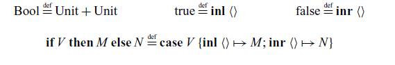
We use the standard encoding of booleans as a sum:
3.2 Handler calculus
We now define ${\lambda_{\textrm{h}}}$
as an extension of
${\lambda_{\textrm{h}}}$
as an extension of ${\lambda_{\textrm{b}}}$
.
${\lambda_{\textrm{b}}}$
.

We assume a fixed effect signature $\Sigma$
that associates types
$\Sigma$
that associates types $\Sigma(\ell)$
to finitely many operation symbols
$\Sigma(\ell)$
to finitely many operation symbols $\ell$
. An operation type
$\ell$
. An operation type $A \to B$
classifies operations that take an argument of type A and return a result of type B. A handler type
$A \to B$
classifies operations that take an argument of type A and return a result of type B. A handler type $C \Rightarrow D$
classifies effect handlers that transform computations of type C into computations of type D. Following Pretnar (Reference Pretnar2015), we assume a global signature for every program. Computations are extended with operation invocation (
$C \Rightarrow D$
classifies effect handlers that transform computations of type C into computations of type D. Following Pretnar (Reference Pretnar2015), we assume a global signature for every program. Computations are extended with operation invocation ( $\mathbf{do}\;\ell\;V$
) and effect handling (
$\mathbf{do}\;\ell\;V$
) and effect handling ( $\mathbf{handle}\; M \;\mathbf{with}\; H$
). Handlers are constructed from a single success clause
$\mathbf{handle}\; M \;\mathbf{with}\; H$
). Handlers are constructed from a single success clause $(\{\mathbf{val}\; x \mapsto M\})$
and an operation clause
$(\{\mathbf{val}\; x \mapsto M\})$
and an operation clause $(\{ \ell \; p \; r \mapsto N \})$
for each operation
$(\{ \ell \; p \; r \mapsto N \})$
for each operation $\ell$
in
$\ell$
in $\Sigma$
; here the x,p,r are considered as bound variables. Following Plotkin & Pretnar (Reference Plotkin and Pretnar2013), we adopt the convention that a handler with missing operation clauses (with respect to
$\Sigma$
; here the x,p,r are considered as bound variables. Following Plotkin & Pretnar (Reference Plotkin and Pretnar2013), we adopt the convention that a handler with missing operation clauses (with respect to $\Sigma$
) is syntactic sugar for one in which all missing clauses perform explicit forwarding:
$\Sigma$
) is syntactic sugar for one in which all missing clauses perform explicit forwarding:
 \[ \{\ell \; p \; r \mapsto \mathbf{let}\; x {{{{{{\leftarrow}}}}}} \mathbf{do} \; \ell \, p \;\mathbf{in}\; r \, x\}\]
The typing rules for ${\lambda_{\textrm{h}}}$
are those of
${\lambda_{\textrm{h}}}$
are those of ${\lambda_{\textrm{b}}}$
(Figure 1) plus three additional rules for operations, handling, and handlers given in Figure 3. The T-Do rule ensures that an operation invocation is only well-typed if the operation
${\lambda_{\textrm{b}}}$
(Figure 1) plus three additional rules for operations, handling, and handlers given in Figure 3. The T-Do rule ensures that an operation invocation is only well-typed if the operation $\ell$
appears in the effect signature
$\ell$
appears in the effect signature $\Sigma$
and the argument type A matches the type of the provided argument V. The result type B determines the type of the invocation. The T-Handle rule types handler application. The T-Handler rule ensures that the bodies of the success clause and the operation clauses all have the output type D. The type of x in the success clause must match the input type C. The type of the parameter p (
$\Sigma$
and the argument type A matches the type of the provided argument V. The result type B determines the type of the invocation. The T-Handle rule types handler application. The T-Handler rule ensures that the bodies of the success clause and the operation clauses all have the output type D. The type of x in the success clause must match the input type C. The type of the parameter p ( $A_\ell$
) and resumption r (
$A_\ell$
) and resumption r ( $B_\ell \to D$
) in operation clause
$B_\ell \to D$
) in operation clause $H^{\ell}$
is determined by the type of
$H^{\ell}$
is determined by the type of $\ell$
; the return type of r is D, as the body of the resumption will itself be handled by H. We write
$\ell$
; the return type of r is D, as the body of the resumption will itself be handled by H. We write $H^{\ell}$
and
$H^{\ell}$
and $H^{\mathrm{val}}$
for projecting success and operation clauses.
$H^{\mathrm{val}}$
for projecting success and operation clauses.

We extend the operational semantics to ${\lambda_{\textrm{h}}}$
. Specifically, we add two new reduction rules: one for handling return values and another for handling operation invocations.
${\lambda_{\textrm{h}}}$
. Specifically, we add two new reduction rules: one for handling return values and another for handling operation invocations.

The first rule invokes the success clause. The second rule handles an operation via the corresponding operation clause.

Fig. 3. Additional typing rules for ${\lambda_{\textrm{h}}}$
.
${\lambda_{\textrm{h}}}$
.
To allow for the evaluation of subterms within $\mathbf{handle}$
expressions, we extend our earlier grammar for evaluation contexts to one for handler contexts:
$\mathbf{handle}$
expressions, we extend our earlier grammar for evaluation contexts to one for handler contexts:
We then replace the S-Lift rule with a corresponding rule for handler contexts.
However, it is critical that the rule S-Op is restricted to pure evaluation contexts ${{{{{{\mathcal{E}}}}}}}$
rather than handler contexts. This ensures that the
${{{{{{\mathcal{E}}}}}}}$
rather than handler contexts. This ensures that the $\mathbf{do}$
invocation is handled by the innermost handler (recalling our convention that all handlers handle all operations). If arbitrary handler contexts
$\mathbf{do}$
invocation is handled by the innermost handler (recalling our convention that all handlers handle all operations). If arbitrary handler contexts ${{{{{{\mathcal{H}}}}}}}$
were permitted in this rule, the semantics would become non-deterministic, as any handler in scope could be selected.
${{{{{{\mathcal{H}}}}}}}$
were permitted in this rule, the semantics would become non-deterministic, as any handler in scope could be selected.
The ancestor-descendant relation for subterm occurrences extends to ${\lambda_{\textrm{h}}}$
in the obvious way.
${\lambda_{\textrm{h}}}$
in the obvious way.
We now characterise normal forms and state the standard type soundness property of ${\lambda_{\textrm{h}}}$
.
${\lambda_{\textrm{h}}}$
.
Definition 1 (Computation normal forms). A computation term N is normal with respect to $\Sigma$
if
$\Sigma$
if $N = \mathbf{return}\;V$
for some V or
$N = \mathbf{return}\;V$
for some V or $N = {{{{{{\mathcal{E}}}}}}}[\mathbf{do}\;\ell\,W]$
for some
$N = {{{{{{\mathcal{E}}}}}}}[\mathbf{do}\;\ell\,W]$
for some $\ell \in dom(\Sigma)$
,
$\ell \in dom(\Sigma)$
, ${{{{{{\mathcal{E}}}}}}}$
, and W.
${{{{{{\mathcal{E}}}}}}}$
, and W.
Theorem 1 (Type Soundness for ${\lambda_{\textrm{h}}}$
) If
${\lambda_{\textrm{h}}}$
) If $ \vdash M : C$
, then either there exists
$ \vdash M : C$
, then either there exists $ \vdash N : C$
such that
$ \vdash N : C$
such that $M {{{{{{\leadsto}}}}}}^\ast N$
and N is normal with respect to
$M {{{{{{\leadsto}}}}}}^\ast N$
and N is normal with respect to $\Sigma$
, or M diverges.
$\Sigma$
, or M diverges.
It is worth observing that our language does not prohibit ‘operation extrusion’: even if we begin with a term in which all $\mathbf{do}$
invocations fall within the scope of a handler, this property need not be preserved by reductions, since a
$\mathbf{do}$
invocations fall within the scope of a handler, this property need not be preserved by reductions, since a $\mathbf{do}$
invocation may pass another
$\mathbf{do}$
invocation may pass another $\mathbf{do}$
to the outermost handler. Such behaviour may be readily ruled out using a type-and-effect system, but this additional machinery is not necessary for our present purposes.
$\mathbf{do}$
to the outermost handler. Such behaviour may be readily ruled out using a type-and-effect system, but this additional machinery is not necessary for our present purposes.
4 Abstract machine semantics
Thus far we have introduced the base calculus ${\lambda_{\textrm{b}}}$
and its extension with effect handlers
${\lambda_{\textrm{b}}}$
and its extension with effect handlers ${\lambda_{\textrm{h}}}$
. For each calculus, we have given a small-step operational semantics which uses a substitution model for evaluation. Whilst this model is semantically pleasing, it falls short of providing a realistic account of practical computation as substitution is an expensive operation. We now develop a more practical model of computation based on an abstract machine semantics.
${\lambda_{\textrm{h}}}$
. For each calculus, we have given a small-step operational semantics which uses a substitution model for evaluation. Whilst this model is semantically pleasing, it falls short of providing a realistic account of practical computation as substitution is an expensive operation. We now develop a more practical model of computation based on an abstract machine semantics.
4.1 Base machine
We choose a CEK-style abstract machine semantics (Felleisen & Friedman, Reference Felleisen and Friedman1987) for ${\lambda _b}$
based on that of Hillerström et al. (Reference Hillerström, Lindley and Longley2020). The CEK machine operates on configurations which are triples of the form
${\lambda _b}$
based on that of Hillerström et al. (Reference Hillerström, Lindley and Longley2020). The CEK machine operates on configurations which are triples of the form ${{{{{{\langle M \mid \gamma \mid \sigma \rangle}}}}}}$
. The first component contains the computation currently being evaluated. The second component contains the environment
${{{{{{\langle M \mid \gamma \mid \sigma \rangle}}}}}}$
. The first component contains the computation currently being evaluated. The second component contains the environment $\gamma$
which binds free variables. The third component contains the continuation which instructs the machine how to proceed once evaluation of the current computation is complete. The syntax of abstract machine states is as follows.
$\gamma$
which binds free variables. The third component contains the continuation which instructs the machine how to proceed once evaluation of the current computation is complete. The syntax of abstract machine states is as follows.

Values consist of function closures, constants, pairs, and left or right tagged values. We refer to continuations of the base machine as pure. A pure continuation is a stack of pure continuation frames. A pure continuation frame $(\gamma, x, N)$
closes a let-binding
$(\gamma, x, N)$
closes a let-binding $\mathbf{let} \;x{{{{{{\leftarrow}}}}}} [~] \;\mathbf{in}\;N$
over environment
$\mathbf{let} \;x{{{{{{\leftarrow}}}}}} [~] \;\mathbf{in}\;N$
over environment $\gamma$
. We write
$\gamma$
. We write ${{{{{{[]}}}}}}$
for an empty pure continuation and
${{{{{{[]}}}}}}$
for an empty pure continuation and $\phi {{{{{{::}}}}}} \sigma$
for the result of pushing the frame
$\phi {{{{{{::}}}}}} \sigma$
for the result of pushing the frame $\phi$
onto
$\phi$
onto $\sigma$
. We use pattern matching to deconstruct pure continuations.
$\sigma$
. We use pattern matching to deconstruct pure continuations.
The abstract machine semantics is given in Figure 4. The transition relation ( ${{{{{{\longrightarrow}}}}}}$
) makes use of the value interpretation (
${{{{{{\longrightarrow}}}}}}$
) makes use of the value interpretation ( $[\![ - ]\!] $
) from value terms to machine values. The machine is initialised by placing a term in a configuration alongside the empty environment (
$[\![ - ]\!] $
) from value terms to machine values. The machine is initialised by placing a term in a configuration alongside the empty environment ( $\emptyset$
) and the identity pure continuation (
$\emptyset$
) and the identity pure continuation ( ${{{{{{[]}}}}}}$
). The rules (M-App), (M-Rec), (M-Const), (M-Split), (M-CaseL), and (M-CaseR) eliminate values. The (M-Let) rule extends the current pure continuation with let bindings. The (M-RetCont) rule extends the environment in the top frame of the pure continuation with a returned value. Given an input of a well-typed closed computation term
${{{{{{[]}}}}}}$
). The rules (M-App), (M-Rec), (M-Const), (M-Split), (M-CaseL), and (M-CaseR) eliminate values. The (M-Let) rule extends the current pure continuation with let bindings. The (M-RetCont) rule extends the environment in the top frame of the pure continuation with a returned value. Given an input of a well-typed closed computation term $ \vdash M : A$
, the machine will either diverge or return a value of type A. A final state is given by a configuration of the form
$ \vdash M : A$
, the machine will either diverge or return a value of type A. A final state is given by a configuration of the form ${{{{{{\langle \mathbf{return}\;V \mid \gamma \mid {{{{{{[]}}}}}} \rangle}}}}}}$
in which case the final return value is given by the denotation
${{{{{{\langle \mathbf{return}\;V \mid \gamma \mid {{{{{{[]}}}}}} \rangle}}}}}}$
in which case the final return value is given by the denotation $[\![ V ]\!] \gamma$
of V under environment
$[\![ V ]\!] \gamma$
of V under environment $\gamma$
.
$\gamma$
.

Fig. 4. Abstract machine semantics for ${\lambda_{\textrm{b}}}$
.
${\lambda_{\textrm{b}}}$
.
Correctness. The base machine faithfully simulates the operational semantics for ${\lambda_{\textrm{b}}}$
; most transitions correspond directly to
${\lambda_{\textrm{b}}}$
; most transitions correspond directly to $\beta$
-reductions, but M-Let performs an administrative step to bring the computation M into evaluation position. We formally state and prove the correspondence in Appendix A, relying on an inverse map
$\beta$
-reductions, but M-Let performs an administrative step to bring the computation M into evaluation position. We formally state and prove the correspondence in Appendix A, relying on an inverse map $(|-|)$
from configurations to terms (Hillerström et al., Reference Hillerström, Lindley and Longley2020).
$(|-|)$
from configurations to terms (Hillerström et al., Reference Hillerström, Lindley and Longley2020).
4.2 Handler machine
We now enrich the ${\lambda_{\textrm{b}}}$
machine to a
${\lambda_{\textrm{b}}}$
machine to a ${\lambda_{\textrm{h}}}$
machine. We extend the syntax as follows.
${\lambda_{\textrm{h}}}$
machine. We extend the syntax as follows.

The notion of configurations changes slightly in that the continuation component is replaced by a generalised continuation $\kappa \in \mathsf{Cont}$
(Hillerström et al., Reference Hillerström, Lindley and Longley2020); a continuation is now a list of resumptions. A resumption is a pair of a pure continuation (as in the base machine) and a handler closure (
$\kappa \in \mathsf{Cont}$
(Hillerström et al., Reference Hillerström, Lindley and Longley2020); a continuation is now a list of resumptions. A resumption is a pair of a pure continuation (as in the base machine) and a handler closure ( $\chi$
). A handler closure consists of an environment and a handler definition, where the former binds the free variables that occur in the latter. The machine is initialised by placing a term in a configuration alongside the empty environment (
$\chi$
). A handler closure consists of an environment and a handler definition, where the former binds the free variables that occur in the latter. The machine is initialised by placing a term in a configuration alongside the empty environment ( $\emptyset$
) and the identity continuation (
$\emptyset$
) and the identity continuation ( $\kappa_0$
). The latter is a singleton list containing the identity resumption, which consists of the identity pure continuation paired with the identity handler closure:
$\kappa_0$
). The latter is a singleton list containing the identity resumption, which consists of the identity pure continuation paired with the identity handler closure:
 \[\kappa_0 \mathrel{\overset{{\mbox{def}}}{=}} [({{{{{{[]}}}}}}, (\emptyset, \{\mathbf{val}\;x \mapsto \mathbf{return}~x\}))]\]
Machine values are augmented to include resumptions as an operation invocation causes the topmost frame of the machine continuation to be reified (and bound to the resumption parameter in the operation clause).
The handler machine adds transition rules for handlers and modifies $(\text{M-L<sc>et</sc>})$
and
$(\text{M-L<sc>et</sc>})$
and $(\text{M-RetCont})$
from the base machine to account for the richer continuation structure. Figure 5 depicts the new and modified rules. The
$(\text{M-RetCont})$
from the base machine to account for the richer continuation structure. Figure 5 depicts the new and modified rules. The $(\text{M-Handle})$
rule pushes a handler closure along with an empty pure continuation onto the continuation stack. The
$(\text{M-Handle})$
rule pushes a handler closure along with an empty pure continuation onto the continuation stack. The $(\text{M-RetHandler})$
rule transfers control to the success clause of the current handler once the pure continuation is empty. The
$(\text{M-RetHandler})$
rule transfers control to the success clause of the current handler once the pure continuation is empty. The $(\text{M-Handle-Op})$
rule transfers control to the matching operation clause on the topmost handler, and during the process it reifies the handler closure. Finally, the
$(\text{M-Handle-Op})$
rule transfers control to the matching operation clause on the topmost handler, and during the process it reifies the handler closure. Finally, the $(\text{M-Resume})$
rule applies a reified handler closure, by pushing it onto the continuation stack. The handler machine has two possible final states: either it yields a value or it gets stuck on an unhandled operation.
$(\text{M-Resume})$
rule applies a reified handler closure, by pushing it onto the continuation stack. The handler machine has two possible final states: either it yields a value or it gets stuck on an unhandled operation.

Fig. 5. Abstract machine semantics for ${\lambda_{\textrm{h}}}$
.
${\lambda_{\textrm{h}}}$
.
Correctness. The handler machine faithfully simulates the operational semantics of ${\lambda_{\textrm{h}}}$
. Extending the result for the base machine, we formally state and prove the correspondence in Appendix B.
${\lambda_{\textrm{h}}}$
. Extending the result for the base machine, we formally state and prove the correspondence in Appendix B.
4.3 Realisability and asymptotic complexity
As witnessed by the work of Hillerström & Lindley (Reference Hillerström and Lindley2016), the machine structures are readily realisable using standard persistent functional data structures. Pure continuations on the base machine and generalised continuations on the handler machine can be implemented using linked lists with a time complexity of ${{{{{{\mathcal{O}}}}}}}(1)$
for the extension operation
${{{{{{\mathcal{O}}}}}}}(1)$
for the extension operation $(\_{{{{{{::}}}}}}\_)$
. The topmost pure continuation on the handler machine may also be extended in time
$(\_{{{{{{::}}}}}}\_)$
. The topmost pure continuation on the handler machine may also be extended in time ${{{{{{\mathcal{O}}}}}}}(1)$
, as extending it only requires reaching under the topmost handler closure. Environments,
${{{{{{\mathcal{O}}}}}}}(1)$
, as extending it only requires reaching under the topmost handler closure. Environments, $\gamma$
, can be realised using a map, with a time complexity of
$\gamma$
, can be realised using a map, with a time complexity of ${{{{{{\mathcal{O}}}}}}}(\log|\gamma|)$
for extension and lookup (Okasaki, Reference Okasaki1999). We can use the same technique to realise label lookup,
${{{{{{\mathcal{O}}}}}}}(\log|\gamma|)$
for extension and lookup (Okasaki, Reference Okasaki1999). We can use the same technique to realise label lookup, $H^{\ell}$
, with time complexity
$H^{\ell}$
, with time complexity ${{{{{{\mathcal{O}}}}}}}(\log|\Sigma|)$
. However, in Section 5.4, we shall work only with a single effect operation, so
${{{{{{\mathcal{O}}}}}}}(\log|\Sigma|)$
. However, in Section 5.4, we shall work only with a single effect operation, so $|\Sigma| = 1$
, meaning that in our analysis we can practically treat label lookup as being a constant time operation.
$|\Sigma| = 1$
, meaning that in our analysis we can practically treat label lookup as being a constant time operation.
The worst-case time complexity of a single machine transition is exhibited by rules which involves the value translation function, $[\![ - ]\!] \gamma$
, as it is defined structurally on values. Its worst-time complexity is exhibited by a nesting of pairs of variables
$[\![ - ]\!] \gamma$
, as it is defined structurally on values. Its worst-time complexity is exhibited by a nesting of pairs of variables $[\![ {{{{{{\langle x_1,{{{{{{\langle x_2,\cdots,{{{{{{\langle x_{n-1},x_n \rangle}}}}}}\cdots \rangle}}}}}} \rangle}}}}}} ]\!] \gamma$
which has complexity
$[\![ {{{{{{\langle x_1,{{{{{{\langle x_2,\cdots,{{{{{{\langle x_{n-1},x_n \rangle}}}}}}\cdots \rangle}}}}}} \rangle}}}}}} ]\!] \gamma$
which has complexity ${{{{{{\mathcal{O}}}}}}}(n\log|\gamma|)$
.
${{{{{{\mathcal{O}}}}}}}(n\log|\gamma|)$
.
Continuation copying. On the handler machine the topmost continuation frame can be copied in constant time due to the persistent runtime and the layout of machine continuations. An alternative design would be to make the runtime non-persistent in which case copying a continuation frame $((\sigma, \chi) {{{{{{::}}}}}} \_)$
would be a
$((\sigma, \chi) {{{{{{::}}}}}} \_)$
would be a ${{{{{{\mathcal{O}}}}}}}(|\sigma| + |\chi|)$
time operation, where
${{{{{{\mathcal{O}}}}}}}(|\sigma| + |\chi|)$
time operation, where $|\chi|$
is the size of the handler closure
$|\chi|$
is the size of the handler closure $\chi$
.
$\chi$
.
Primitive operations on naturals. Our model assumes that arithmetic operations on arbitrary natural numbers take ${{{{{{\mathcal{O}}}}}}}(1)$
time. This is common practice in the study of algorithms when the main interest lies elsewhere (Cormen et al., Reference Cormen, Leiserson, Rivest and Stein2009, Section 2.2). If desired, one could adopt a more refined cost model that accounted for the bit-level complexity of arithmetic operations; however, doing so would have the same impact on both of the situations we are wishing to compare, and thus would add nothing but noise to the overall analysis.
${{{{{{\mathcal{O}}}}}}}(1)$
time. This is common practice in the study of algorithms when the main interest lies elsewhere (Cormen et al., Reference Cormen, Leiserson, Rivest and Stein2009, Section 2.2). If desired, one could adopt a more refined cost model that accounted for the bit-level complexity of arithmetic operations; however, doing so would have the same impact on both of the situations we are wishing to compare, and thus would add nothing but noise to the overall analysis.
5 Predicates, decision trees and generic count
We now come to the crux of the paper. In this section and the next, we prove that ${\lambda_{\textrm{h}}}$
supports implementations of certain operations with an asymptotic runtime bound that cannot be achieved in
${\lambda_{\textrm{h}}}$
supports implementations of certain operations with an asymptotic runtime bound that cannot be achieved in ${\lambda_{\textrm{b}}}$
(Section 8). While the positive half of this claim essentially consolidates a known piece of folklore, the negative half appears to be new. To establish our result, it will suffice to exhibit a single ‘efficient’ program in
${\lambda_{\textrm{b}}}$
(Section 8). While the positive half of this claim essentially consolidates a known piece of folklore, the negative half appears to be new. To establish our result, it will suffice to exhibit a single ‘efficient’ program in ${\lambda_{\textrm{h}}}$
, then show that no equivalent program in
${\lambda_{\textrm{h}}}$
, then show that no equivalent program in ${\lambda_{\textrm{b}}}$
can achieve the same asymptotic efficiency. We take generic search as our example.
${\lambda_{\textrm{b}}}$
can achieve the same asymptotic efficiency. We take generic search as our example.
Generic search is a modular search procedure that takes as input a predicate P on some multi-dimensional search space and finds all points of the space satisfying P. Generic search is agnostic to the specific instantiation of P, and as a result is applicable across a wide spectrum of domains. Classic examples such as Sudoku solving (Bird, Reference Bird2006), the n-queens problem (Bell & Stevens, Reference Bell and Stevens2009) and graph colouring can be cast as instances of generic search, and similar ideas have been explored in connection with exact real integration (Simpson, Reference Simpson1998; Daniels, Reference Daniels2016).
For simplicity, we will restrict attention to search spaces of the form ${{{{{{\mathbb{B}}}}}}}^n$
, the set of bit vectors of length n. To exhibit our phenomenon in the simplest possible setting, we shall actually focus on the generic count problem: given a predicate P on some
${{{{{{\mathbb{B}}}}}}}^n$
, the set of bit vectors of length n. To exhibit our phenomenon in the simplest possible setting, we shall actually focus on the generic count problem: given a predicate P on some ${{{{{{\mathbb{B}}}}}}}^n$
, return the number of points of
${{{{{{\mathbb{B}}}}}}}^n$
, return the number of points of ${{{{{{\mathbb{B}}}}}}}^n$
satisfying P. However, we shall explain why our results are also applicable to generic search proper.
${{{{{{\mathbb{B}}}}}}}^n$
satisfying P. However, we shall explain why our results are also applicable to generic search proper.
We shall view ${{{{{{\mathbb{B}}}}}}}^n$
as the set of functions
${{{{{{\mathbb{B}}}}}}}^n$
as the set of functions ${{{{{{\mathbb{N}}}}}}}_n \to {{{{{{\mathbb{B}}}}}}}$
, where
${{{{{{\mathbb{N}}}}}}}_n \to {{{{{{\mathbb{B}}}}}}}$
, where ${{{{{{\mathbb{N}}}}}}}_n \mathrel{\overset{{\mbox{def}}}{=}} \{0,\dots,n-1\}$
. In both
${{{{{{\mathbb{N}}}}}}}_n \mathrel{\overset{{\mbox{def}}}{=}} \{0,\dots,n-1\}$
. In both ${\lambda_{\textrm{b}}}$
and
${\lambda_{\textrm{b}}}$
and ${\lambda_{\textrm{h}}}$
we may represent such functions by terms of type
${\lambda_{\textrm{h}}}$
we may represent such functions by terms of type $\mathrm{Nat} \to \mathrm{Bool}$
. We will often informally write
$\mathrm{Nat} \to \mathrm{Bool}$
. We will often informally write $\mathrm{Nat}_n$
in place of Nat to indicate that only the values
$\mathrm{Nat}_n$
in place of Nat to indicate that only the values $0,\dots,n-1$
are relevant, but this convention has no formal status since our setup does not support dependent types.
$0,\dots,n-1$
are relevant, but this convention has no formal status since our setup does not support dependent types.
To summarise, in both ${\lambda_{\textrm{b}}}$
and
${\lambda_{\textrm{b}}}$
and ${\lambda_{\textrm{h}}}$
we will be working with the types
${\lambda_{\textrm{h}}}$
we will be working with the types

and will be looking for programs
 \[ \mathrm{count}_n : \mathrm{Predicate}_n \to \mathrm{Nat}\]
such that for suitable terms P representing semantic predicates $\Pi: {{{{{{\mathbb{B}}}}}}}^n \to {{{{{{\mathbb{B}}}}}}}$
,
$\Pi: {{{{{{\mathbb{B}}}}}}}^n \to {{{{{{\mathbb{B}}}}}}}$
, $\mathrm{count}_n~P$
finds the number of points of
$\mathrm{count}_n~P$
finds the number of points of ${{{{{{\mathbb{B}}}}}}}^n$
satisfying
${{{{{{\mathbb{B}}}}}}}^n$
satisfying $\Pi$
.
$\Pi$
.
Before formalising these ideas more closely, let us look at some examples, which will also illustrate the machinery of decision trees that we will be using.
5.1 Examples of points, predicates and trees
Consider first the following terms of type Point:
(Here $\bot$
is the diverging term
$\bot$
is the diverging term $(\mathbf{rec}\; f\,i.f\,i)\,{\langle \rangle}$
.) Then
$(\mathbf{rec}\; f\,i.f\,i)\,{\langle \rangle}$
.) Then $\mathrm{q}_0$
represents
$\mathrm{q}_0$
represents $\langle{\mathrm{true},\dots,\mathrm{true}}\rangle \in {{{{{{\mathbb{B}}}}}}}^n$
for any n;
$\langle{\mathrm{true},\dots,\mathrm{true}}\rangle \in {{{{{{\mathbb{B}}}}}}}^n$
for any n; $\mathrm{q}_1$
represents
$\mathrm{q}_1$
represents $\langle{\mathrm{true},\mathrm{false},\dots,\mathrm{false}}\rangle \in {{{{{{\mathbb{B}}}}}}}^n$
for any
$\langle{\mathrm{true},\mathrm{false},\dots,\mathrm{false}}\rangle \in {{{{{{\mathbb{B}}}}}}}^n$
for any $n \geq 1$
; and
$n \geq 1$
; and $\mathrm{q}_2$
represents
$\mathrm{q}_2$
represents $\langle{\mathrm{true},\mathrm{false}}\rangle \in {{{{{{\mathbb{B}}}}}}}^2$
.
$\langle{\mathrm{true},\mathrm{false}}\rangle \in {{{{{{\mathbb{B}}}}}}}^2$
.
Next some predicates. First, the following terms all represent the constant true predicate ${{{{{{\mathbb{B}}}}}}}^2 \to {{{{{{\mathbb{B}}}}}}}$
:
${{{{{{\mathbb{B}}}}}}}^2 \to {{{{{{\mathbb{B}}}}}}}$
:
These illustrate that in the course of evaluating a predicate term P at a point q, for each $i<n$
the value of q at i may be inspected zero, one or many times.
$i<n$
the value of q at i may be inspected zero, one or many times.
Likewise, the following all represent the ‘identity’ predicate ${{{{{{\mathbb{B}}}}}}}^1 \to {{{{{{\mathbb{B}}}}}}}$
, in a sense to be made precise below (here
${{{{{{\mathbb{B}}}}}}}^1 \to {{{{{{\mathbb{B}}}}}}}$
, in a sense to be made precise below (here $\&\&$
is shortcut ‘and’):
$\&\&$
is shortcut ‘and’):
Slightly more interestingly, for each n we have the following program which determines whether a point contains an odd number of true components:
 \[ \mathrm{Odd}_n \mathrel{\overset{{\mbox{def}}}{=}} \lambda q.\, \mathrm{fold}\otimes\mathrm{false}~(\mathrm{map}~q~[0,\dots,n-1])\]
Here fold and map are the standard combinators on lists, and $\otimes$
is exclusive-or. Applying
$\otimes$
is exclusive-or. Applying $\mathrm{Odd}_2$
to
$\mathrm{Odd}_2$
to $\mathrm{q}_0$
yields false; applying it to
$\mathrm{q}_0$
yields false; applying it to $\mathrm{q}_1$
or
$\mathrm{q}_1$
or $\mathrm{q}_2$
yields true.
$\mathrm{q}_2$
yields true.
We can think of a predicate term P as participating in a ‘dialogue’ with a given point $Q : \mathrm{Point}_n$
. The predicate may query Q at some coordinate k; Q may respond with true or false and this returned value may influence the future course of the dialogue. After zero or more such query/response pairs, the predicate may return a final answer (true or false).
$Q : \mathrm{Point}_n$
. The predicate may query Q at some coordinate k; Q may respond with true or false and this returned value may influence the future course of the dialogue. After zero or more such query/response pairs, the predicate may return a final answer (true or false).
The set of possible dialogues with a given term P may be organised in an obvious way into an unrooted binary decision tree, in which each internal node is labelled with a query $\mathord{?} k$
(with
$\mathord{?} k$
(with $k<n$
), and with left and right branches corresponding to the responses true, false respectively. Any point will thus determine a path through the tree, and each leaf is labelled with an answer
$k<n$
), and with left and right branches corresponding to the responses true, false respectively. Any point will thus determine a path through the tree, and each leaf is labelled with an answer $\mathord{!} \mathrm{true}$
or
$\mathord{!} \mathrm{true}$
or $\mathord{!} \mathrm{false}$
according to whether the corresponding point or points satisfy the predicate.
$\mathord{!} \mathrm{false}$
according to whether the corresponding point or points satisfy the predicate.
Decision trees for a sample of the above predicate terms are depicted in Figure 6; the relevant formal definitions are given in the next subsection. In the case of $\mathrm{I}_2$
, one of the
$\mathrm{I}_2$
, one of the $\mathord{!} \mathrm{false}$
leaves will be ‘unreachable’ if we are working in
$\mathord{!} \mathrm{false}$
leaves will be ‘unreachable’ if we are working in ${\lambda_{\textrm{b}}}$
(but reachable in a language supporting mutable state).
${\lambda_{\textrm{b}}}$
(but reachable in a language supporting mutable state).

Fig. 6. Examples of decision trees.
We think of the edges in the tree as corresponding to portions of computation undertaken by P between queries, or before delivering the final answer. The tree is unrooted (i.e. starts with an edge rather than a node) because in the evaluation of $P\,Q$
there is potentially some ‘thinking’ done by P even before the first query or answer is reached. For the purpose of our runtime analysis, we will also consider timed variants of these decision trees, in which each edge is labelled with the number of computation steps involved.
$P\,Q$
there is potentially some ‘thinking’ done by P even before the first query or answer is reached. For the purpose of our runtime analysis, we will also consider timed variants of these decision trees, in which each edge is labelled with the number of computation steps involved.
It is possible that for a given P, the construction of a decision tree may hit trouble, because at some stage P either goes undefined or gets stuck at an unhandled operation. It is also possible that the decision tree is infinite because P can keep asking queries forever. However, we shall be restricting our attention to terms representing total predicates: those with finite decision trees in which every path leads to a leaf.
In order to present our complexity results in a simple and clear form, we will give special prominence to certain well-behaved decision trees. For $n \in {{{{{{\mathbb{N}}}}}}}$
, we shall say a tree is n-standard if it is total (i.e. every maximal path leads to a leaf labelled with an answer) and along any path to a leaf, each coordinate
$n \in {{{{{{\mathbb{N}}}}}}}$
, we shall say a tree is n-standard if it is total (i.e. every maximal path leads to a leaf labelled with an answer) and along any path to a leaf, each coordinate $k<n$
is queried once and only once. Thus, an n-standard decision tree is a complete binary tree of depth
$k<n$
is queried once and only once. Thus, an n-standard decision tree is a complete binary tree of depth $n+1$
, with
$n+1$
, with $2^n - 1$
internal nodes and
$2^n - 1$
internal nodes and $2^n$
leaves. However, there is no constraint on the order of the queries, which indeed may vary from one path to another. One pleasing property of this notion is that for a predicate term with an n-standard decision tree, the number of points in
$2^n$
leaves. However, there is no constraint on the order of the queries, which indeed may vary from one path to another. One pleasing property of this notion is that for a predicate term with an n-standard decision tree, the number of points in ${{{{{{\mathbb{B}}}}}}}^n$
satisfying the predicate is precisely the number of
${{{{{{\mathbb{B}}}}}}}^n$
satisfying the predicate is precisely the number of $\mathord{!} \mathrm{true}$
leaves in the tree.
$\mathord{!} \mathrm{true}$
leaves in the tree.
Of the examples we have given, the tree for $\mathrm{T}_0$
is 0-standard; those for
$\mathrm{T}_0$
is 0-standard; those for $\mathrm{I}_0$
and
$\mathrm{I}_0$
and $\mathrm{I}_1$
are 1-standard; that for
$\mathrm{I}_1$
are 1-standard; that for $\mathrm{Odd}_n$
is n-standard; and the rest are not n-standard for any n.
$\mathrm{Odd}_n$
is n-standard; and the rest are not n-standard for any n.
5.2 Formal definitions
We now formalise the above notions. We will present our definitions in the setting of ${\lambda_{\textrm{h}}}$
, but everything can clearly be relativised to
${\lambda_{\textrm{h}}}$
, but everything can clearly be relativised to ${\lambda_{\textrm{b}}}$
with no change to the meaning in the case of
${\lambda_{\textrm{b}}}$
with no change to the meaning in the case of ${\lambda_{\textrm{b}}}$
terms. For the purpose of this subsection, we fix
${\lambda_{\textrm{b}}}$
terms. For the purpose of this subsection, we fix $n \in {{{{{{\mathbb{N}}}}}}}$
, set
$n \in {{{{{{\mathbb{N}}}}}}}$
, set ${{{{{{\mathbb{N}}}}}}}_n \mathrel{\overset{{\mbox{def}}}{=}} \{0,\ldots,n-1\}$
, and use k to range over
${{{{{{\mathbb{N}}}}}}}_n \mathrel{\overset{{\mbox{def}}}{=}} \{0,\ldots,n-1\}$
, and use k to range over ${{{{{{\mathbb{N}}}}}}}_n$
. We write
${{{{{{\mathbb{N}}}}}}}_n$
. We write ${{{{{{\mathbb{B}}}}}}}$
for the set of booleans, which we shall identify with the (encoded) boolean values of
${{{{{{\mathbb{B}}}}}}}$
for the set of booleans, which we shall identify with the (encoded) boolean values of ${\lambda_{\textrm{h}}}$
, and use b to range over
${\lambda_{\textrm{h}}}$
, and use b to range over ${{{{{{\mathbb{B}}}}}}}$
.
${{{{{{\mathbb{B}}}}}}}$
.
As suggested by the foregoing discussion, we will need to work with both syntax and semantics. For points, the relevant definitions are as follows.
Definition 2 (points). A closed value $Q : \mathrm{Point}$
is said to be a syntactic n-point if:
$Q : \mathrm{Point}$
is said to be a syntactic n-point if:
 \[ \forall k \in {{{{{{\mathbb{N}}}}}}}_n.\,\exists b \in {{{{{{\mathbb{B}}}}}}}.~ Q~k {{{{{{\leadsto}}}}}}^\ast \mathbf{return}\;b \]
A semantic n-point $\pi$
is simply a mathematical function
$\pi$
is simply a mathematical function $\pi: {{{{{{\mathbb{N}}}}}}}_n \to {{{{{{\mathbb{B}}}}}}}$
. (We shall also write
$\pi: {{{{{{\mathbb{N}}}}}}}_n \to {{{{{{\mathbb{B}}}}}}}$
. (We shall also write $\pi \in {{{{{{\mathbb{B}}}}}}}^n$
.) Any syntactic n-point Q is said to denote the semantic n-point
$\pi \in {{{{{{\mathbb{B}}}}}}}^n$
.) Any syntactic n-point Q is said to denote the semantic n-point $[\![ Q ]\!] $
given by
$[\![ Q ]\!] $
given by
 \[ \forall k \in {{{{{{\mathbb{N}}}}}}}_n,\, b \in {{{{{{\mathbb{B}}}}}}}.~ [\![ Q ]\!] (k) = b \,\Leftrightarrow\, Q~k {{{{{{\leadsto}}}}}}^\ast \mathbf{return}\;b \]
Any two syntactic n-points Q and Q’ are said to be distinct if $[\![ Q ]\!] \neq [\![ Q' ]\!] $
.
$[\![ Q ]\!] \neq [\![ Q' ]\!] $
.
By default, the unqualified term n-point will from now on refer to syntactic n-points.
Likewise, we wish to work with predicates both syntactically and semantically. By a semantic n-predicate, we shall mean simply a mathematical function $\Pi: {{{{{{\mathbb{B}}}}}}}^n \to {{{{{{\mathbb{B}}}}}}}$
. One slick way to define syntactic n-predicates would be as closed terms
$\Pi: {{{{{{\mathbb{B}}}}}}}^n \to {{{{{{\mathbb{B}}}}}}}$
. One slick way to define syntactic n-predicates would be as closed terms $P:\mathrm{Predicate}$
such that for every n-point Q,
$P:\mathrm{Predicate}$
such that for every n-point Q, $P\,Q$
evaluates to either
$P\,Q$
evaluates to either $\mathbf{return}\;\mathrm{true}$
or
$\mathbf{return}\;\mathrm{true}$
or $\mathbf{return}\;\mathrm{false}$
. For our purposes, however, we shall favour an approach to n-predicates via decision trees, which will yield more information on their behaviour.
$\mathbf{return}\;\mathrm{false}$
. For our purposes, however, we shall favour an approach to n-predicates via decision trees, which will yield more information on their behaviour.
We will model decision trees as certain partial functions from addresses to labels. An address will specify the position of a node in the tree via the path that leads to it, while a label will represent the information present at a node. Formally:
Definition 3 (untimed decision tree).
-
(i) The address set
$\mathsf{Addr}$
is simply the set
${{{{{{\mathbb{B}}}}}}}^\ast$
of finite lists of booleans. If
$bs,bs' \in \mathsf{Addr}$
, we write
$bs \sqsubseteq bs'$
(resp.
$bs \sqsubset bs'$
) to mean that bs is a prefix (resp. proper prefix) of bs’. -
(ii) The label set
$\mathsf{Lab}$
consists of queries parameterised by a natural number and answers parameterised by a boolean:
\[ \mathsf{Lab} \mathrel{\overset{{\mbox{def}}}{=}} \{\mathord{?} k \mid k \in {{{{{{\mathbb{N}}}}}}} \} \cup \{\mathord{!} b \mid b \in {{{{{{\mathbb{B}}}}}}} \} \]
-
(iii) An (untimed) decision tree is a partial function
$\tau : \mathsf{Addr}\rightharpoonup \mathsf{Lab}$
such that:-
The domain of
$\tau$
(written
$dom(\tau)$
) is prefix closed. -
Answer nodes are always leaves: if
$\tau(bs) = \mathord{!} b$
then
$\tau(bs')$
is undefined whenever
$bs \sqsubset bs'$
.
-


As our goal is to reason about the time complexity of generic count programs and their predicates, it is also helpful to decorate decision trees with timing data that records the number of machine steps taken for each piece of computation performed by a predicate:
Definition 4 (timed decision tree). A timed decision tree is a partial function $\tau : \mathsf{Addr} \rightharpoonup\mathsf{Lab} \times {{{{{{\mathbb{N}}}}}}}$
such that its first projection
$\tau : \mathsf{Addr} \rightharpoonup\mathsf{Lab} \times {{{{{{\mathbb{N}}}}}}}$
such that its first projection $bs \mapsto \tau(bs).1$
is a decision tree. We write
$bs \mapsto \tau(bs).1$
is a decision tree. We write $\mathsf{labs}(\tau)$
for the first projection (
$\mathsf{labs}(\tau)$
for the first projection ( $bs \mapsto \tau(bs).1$
) and
$bs \mapsto \tau(bs).1$
) and $\mathsf{steps}(\tau)$
for the second projection (
$\mathsf{steps}(\tau)$
for the second projection ( $bs \mapsto \tau(bs).2$
) of a timed decision tree.
$bs \mapsto \tau(bs).2$
) of a timed decision tree.
Here we think of $\mathsf{steps}(\tau)(bs)$
as the computation time associated with the edge whose target is the node addressed by bs.
$\mathsf{steps}(\tau)(bs)$
as the computation time associated with the edge whose target is the node addressed by bs.
We now come to the method for associating a specific tree with a given term P. One may think of this as a kind of denotational semantics, but here we shall extract a tree from a term by purely operational means using our abstract machine model. The key idea is to try applying P to a distinguished free variable $q: \mathrm{Point}$
, which we think of as an ‘abstract point’. Whenever P wants to interrogate its argument at some index i, the computation will get stuck at some term
$q: \mathrm{Point}$
, which we think of as an ‘abstract point’. Whenever P wants to interrogate its argument at some index i, the computation will get stuck at some term $q\,i$
: this both flags up the presence of a query node in the decision tree, and allows us to explore the subsequent behaviour under both possible responses to this query.
$q\,i$
: this both flags up the presence of a query node in the decision tree, and allows us to explore the subsequent behaviour under both possible responses to this query.
Our definition captures this idea using abstract machine configurations. We write ${\mathrm{Conf}}_q$
for the set of
${\mathrm{Conf}}_q$
for the set of $\lambda_h$
configurations possibly involving q (but no other free variables). We write
$\lambda_h$
configurations possibly involving q (but no other free variables). We write $a \simeq b$
for Kleene equality: either both a and b are undefined or both are defined and
$a \simeq b$
for Kleene equality: either both a and b are undefined or both are defined and $a = b$
.
$a = b$
.
It is convenient to define the timed tree and then extract the untimed one from it:
Definition 5.
-
(i) Define
$\mathcal{T}: {\mathrm{Conf}}_q \to \mathsf{Addr} \rightharpoonup (\mathsf{Lab} \times {{{{{{\mathbb{N}}}}}}})$
to be the minimal family of partial functions satisfying the following equations:Here
$\mathrm{inc}(\ell, s) = (\ell, s + 1)$
, and in all of the above equations
$\gamma(q) = \gamma'(q) = q$
. Clearly
$\mathcal{T}(\mathcal{C})$
is a timed decision tree for any
$\mathcal{C} \in {\mathrm{Conf}}_q$
. -
(ii) The timed decision tree of a computation term is obtained by placing it in the initial configuration:
$\mathcal{T}(M) \mathrel{\overset{{\mbox{def}}}{=}} \mathcal{T}({{{{{{\langle M, \emptyset[q \mapsto q], \kappa_0 \rangle}}}}}})$
. -
(iii) The timed decision tree of a closed value
$P:\mathrm{Predicate}$
is
$\mathcal{T}(P\,q)$
. Since q plays the role of a dummy argument, we will usually omit it and write
$\mathcal{T}(P)$
for
$\mathcal{T}(P\,q)$
. -
(iv) The untimed decision tree
$\mathcal{U}(P)$
is obtained from
$\mathcal{T}(P)$
via first projection:
$\mathcal{U}(P) = \mathsf{labs}(\mathcal{T}(P))$
.


If the execution of a configuration $\mathcal{C}$
runs forever or gets stuck at an unhandled operation, then
$\mathcal{C}$
runs forever or gets stuck at an unhandled operation, then $\mathcal{T}(\mathcal{C})(bs)$
will be undefined for all bs. Although this is admitted by our definition of decision tree, we wish to exclude such behaviours for the terms we accept as valid predicates. Specifically, we frame the following definition:
$\mathcal{T}(\mathcal{C})(bs)$
will be undefined for all bs. Although this is admitted by our definition of decision tree, we wish to exclude such behaviours for the terms we accept as valid predicates. Specifically, we frame the following definition:
Definition 6 A decision tree $\tau$
is an n-predicate tree if it satisfies the following:
$\tau$
is an n-predicate tree if it satisfies the following:
-
For every query
$\mathord{?} k$
appearing in
$\tau$
, we have
$k \in {{{{{{\mathbb{N}}}}}}}_n$
. -
Every query node has both children present:
\[ \forall bs \in \mathsf{Addr},\, k \in {{{{{{\mathbb{N}}}}}}}_n,\, b \in {{{{{{\mathbb{B}}}}}}}.~ \tau(bs) = \mathord{?} k \Rightarrow {{{{{{bs \mathbin{+\!\!+} [b]}}}}}} \in dom(\tau) \]
-
All paths in
$\tau$
are finite (so every maximal path terminates in an answer node).


A closed term $P: \mathrm{Predicate}$
is a (syntactic) n-predicate if
$P: \mathrm{Predicate}$
is a (syntactic) n-predicate if $\mathcal{U}(P)$
is an n-predicate tree.
$\mathcal{U}(P)$
is an n-predicate tree.
If $\tau$
is an n-predicate tree, clearly any semantic n-point
$\tau$
is an n-predicate tree, clearly any semantic n-point $\pi$
gives rise to a path
$\pi$
gives rise to a path $b_0 b_1 \dots $
through
$b_0 b_1 \dots $
through $\tau$
, given inductively by
$\tau$
, given inductively by
 \[ \forall j.~ \mbox{if~} \tau(b_0\dots b_{j-1}) = \mathord{?} k_j \mbox{~then~} b_j = \pi(k_j) \]
This path will terminate at some answer node $b_0 b_1 \dots b_{r-1}$
of
$b_0 b_1 \dots b_{r-1}$
of $\tau$
, and we may write
$\tau$
, and we may write $\tau \bullet \pi \in {{{{{{\mathbb{B}}}}}}}$
for the answer at this leaf.
$\tau \bullet \pi \in {{{{{{\mathbb{B}}}}}}}$
for the answer at this leaf.
Proposition 1. If P is an n-predicate and Q is an n-point, then $P\,Q {{{{{{\leadsto}}}}}}^\ast \mathbf{return}\;b$
where
$P\,Q {{{{{{\leadsto}}}}}}^\ast \mathbf{return}\;b$
where $b = \mathcal{U}(P) \bullet [\![ Q ]\!] $
.
$b = \mathcal{U}(P) \bullet [\![ Q ]\!] $
.
Proof By interleaving the computation for the relevant path through $\mathcal{U}(P)$
with computations for queries to Q, and appealing to the correspondence between the small-step reduction and abstract machine semantics. We omit the routine details.
$\mathcal{U}(P)$
with computations for queries to Q, and appealing to the correspondence between the small-step reduction and abstract machine semantics. We omit the routine details.
It is thus natural to define the denotation of an n-predicate P to be the semantic n-predicate $[\![ P ]\!] $
given by
$[\![ P ]\!] $
given by $[\![ P ]\!] (\pi) = \mathcal{U}(P) \bullet \pi$
.
$[\![ P ]\!] (\pi) = \mathcal{U}(P) \bullet \pi$
.
As mentioned earlier, we shall also be interested in a more constrained class of trees and predicates:
Definition 7 (standard trees and predicates). An n-predicate tree $\tau$
is said to be n-standard if the following hold:
$\tau$
is said to be n-standard if the following hold:
-
The domain of
$\tau$
is precisely
$\mathsf{Addr}_n$
, the set of bit vectors of length
$\leq n$
. -
There are no repeated queries along any path in
$\tau$
:
\[ \forall bs, bs' \in dom(\tau),\, k \in {{{{{{\mathbb{N}}}}}}}_n.~ bs \sqsubseteq bs' \wedge \tau(bs)=\tau(bs')=\mathord{?} k \Rightarrow bs=bs' \]


A timed decision tree $\tau$
is n-standard if its underlying untimed decision tree
$\tau$
is n-standard if its underlying untimed decision tree $\mathsf{labs}(\tau)$
is too. An n-predicate P is n-standard if
$\mathsf{labs}(\tau)$
is too. An n-predicate P is n-standard if $\mathcal{U}(P)$
is n-standard.
$\mathcal{U}(P)$
is n-standard.
Clearly, in an n-standard tree, each of the n queries $\mathord{?} 0,\dots, \mathord{?}(n-1)$
appears exactly once on the path to any leaf, and there are
$\mathord{?} 0,\dots, \mathord{?}(n-1)$
appears exactly once on the path to any leaf, and there are $2^n$
leaves, all of them answer nodes.
$2^n$
leaves, all of them answer nodes.
It is also clear how for any n-standard tree $\tau$
we may construct a predicate P that denotes it, simply by mirroring the structure of
$\tau$
we may construct a predicate P that denotes it, simply by mirroring the structure of $\tau$
with nested
$\tau$
with nested $\mathbf{if}$
expressions:
$\mathbf{if}$
expressions:
Definition 8 (canonical standard predicates). Given an n-standard tree $\tau$
, we may associate to each address
$\tau$
, we may associate to each address $bs \in dom(\tau)$
a
$bs \in dom(\tau)$
a $\lambda_b$
term
$\lambda_b$
term $T_q(\tau,bs)$
(with free variable
$T_q(\tau,bs)$
(with free variable $q : \mathrm{Point}$
) by reverse induction on the length of bs:
$q : \mathrm{Point}$
) by reverse induction on the length of bs:

We then define
 \[ P(\tau) ~=~ \lambda q.\; T_q(\tau,[]) \]
(so that clearly $\mathcal{U}(P(\tau)) = \tau$
), and call
$\mathcal{U}(P(\tau)) = \tau$
), and call $P(\tau)$
the canonical n-standard predicate for
$P(\tau)$
the canonical n-standard predicate for $\tau$
.
$\tau$
.
In practice, we will omit the subscript q from uses of T.
Note that the use of lists here is entirely at the meta-level, and none of the terms $T(\tau,bs)$
themselves involve list data. Because of their simple, standardised form, canonical n-standard predicates will play a useful role in our lower bound analysis in Section 8.
$T(\tau,bs)$
themselves involve list data. Because of their simple, standardised form, canonical n-standard predicates will play a useful role in our lower bound analysis in Section 8.
5.3 Specification of counting programs
We can now specify what it means for a program $K : \mathrm{Predicate} \to \mathrm{Nat}$
to implement counting.
$K : \mathrm{Predicate} \to \mathrm{Nat}$
to implement counting.
Definition 9.
-
(i) The count of a semantic n-predicate
$\Pi$
, written
$\sharp \Pi$
, is simply the number of semantic n-points
$\pi \in {{{{{{\mathbb{B}}}}}}}^n$
for which
$\Pi(\pi)=\mathrm{true}$
. -
(ii) If P is any n-predicate, we say that K correctly counts P if
$K\,P {{{{{{\leadsto}}}}}}^\ast \mathbf{return}\;m$
, where
$m = \sharp [\![ P ]\!] $
.


This definition gives us the flexibility to talk about counting programs that operate on various classes of predicates, allowing us to state our results in their strongest natural form. On the positive side, we shall shortly see that there is a single ‘efficient’ program in ${\lambda_{\textrm{h}}}$
that correctly counts all n-standard
${\lambda_{\textrm{h}}}$
that correctly counts all n-standard $\lambda_h$
predicates for every n; in Section 6.1 we improve this to one that correctly counts all n-predicates of
$\lambda_h$
predicates for every n; in Section 6.1 we improve this to one that correctly counts all n-predicates of $\lambda_h$
. On the negative side, we shall show that an n-indexed family of counting programs written in
$\lambda_h$
. On the negative side, we shall show that an n-indexed family of counting programs written in ${\lambda_{\textrm{b}}}$
, even if only required to work correctly on canonical n-standard
${\lambda_{\textrm{b}}}$
, even if only required to work correctly on canonical n-standard $\lambda_b$
predicates, can never compete with our
$\lambda_b$
predicates, can never compete with our ${\lambda_{\textrm{h}}}$
program for asymptotic efficiency even in the most favourable cases.
${\lambda_{\textrm{h}}}$
program for asymptotic efficiency even in the most favourable cases.
5.4 Efficient generic count with effects
We now present the simplest version of our effectful implementation of counting: one that works on n-standard predicates.
Our program uses a variation of the handler for nondeterministic computation that we gave in Section 2. The main idea is to implement points as ‘nondeterministic computations’ using the Branch operation such that the handler may respond to every query twice, by invoking the provided resumption with true and subsequently false. The key insight is that the resumption restarts computation at the invocation site of Branch, meaning that prior computation performed by the predicate need not be repeated. In other words, the resumption ensures that common portions of computations prior to any query are shared between both branches.
We assert that $\mathrm{Branch} : \mathrm{Unit} \to \mathrm{Bool} \in \Sigma$
is a distinguished operation that may not be handled in the definition of any input predicate (it has to be forwarded according to the default convention). The algorithm is then as follows.
$\mathrm{Branch} : \mathrm{Unit} \to \mathrm{Bool} \in \Sigma$
is a distinguished operation that may not be handled in the definition of any input predicate (it has to be forwarded according to the default convention). The algorithm is then as follows.

The handler applies predicate pred to a single ‘generic point’ defined using Branch. The boolean return value is interpreted as a single solution, whilst Branch is interpreted by alternately supplying true and false to the resumption and summing the results. The sharing enabled by the use of the resumption is exactly the ‘magic’ we need to make it possible to implement generic count more efficiently in ${\lambda_{\textrm{h}}}$
than in
${\lambda_{\textrm{h}}}$
than in ${\lambda_{\textrm{b}}}$
. A curious feature of effcount is that it works for all n-standard predicates without having to know the value of n.
${\lambda_{\textrm{b}}}$
. A curious feature of effcount is that it works for all n-standard predicates without having to know the value of n.
We may now articulate the crucial correctness and efficiency properties of effcount.
Theorem 2. The following hold for any $n \in {{{{{{\mathbb{N}}}}}}}$
and any n-standard predicate P of
$n \in {{{{{{\mathbb{N}}}}}}}$
and any n-standard predicate P of ${\lambda_{\textrm{h}}}$
:
${\lambda_{\textrm{h}}}$
:
-
1. effcount correctly counts P.
-
2. The number of machine steps required to evaluate
$\mathrm{effcount}~P$
is
\[ \left( \displaystyle\sum_{bs \in \mathsf{Addr}_n} \mathsf{steps}(\mathcal{T}(P))(bs) \right) ~+~ {{{{{{\mathcal{O}}}}}}}(2^n) \]


Proof [Outline.] Suppose $bs \in \mathsf{Addr}_n$
, with length j. From the construction of
$bs \in \mathsf{Addr}_n$
, with length j. From the construction of $\mathcal{T}(P)$
, one may easily read off a configuration
$\mathcal{T}(P)$
, one may easily read off a configuration $\mathcal{C}_{bs}$
whose execution is expected to compute the count for the subtree below node bs, and we can explicitly describe the form
$\mathcal{C}_{bs}$
whose execution is expected to compute the count for the subtree below node bs, and we can explicitly describe the form $\mathcal{C}_{bs}$
will have. We write
$\mathcal{C}_{bs}$
will have. We write $\mathrm{Hyp}(bs)$
for the claim that
$\mathrm{Hyp}(bs)$
for the claim that $\mathcal{C}_{bs}$
correctly counts this subtree and does so within the following number of steps:
$\mathcal{C}_{bs}$
correctly counts this subtree and does so within the following number of steps:
 \[ \left( \displaystyle\sum_{bs' \in \mathsf{Addr}_n,\; bs' \sqsupset bs} \mathsf{steps}(\mathcal{T}(P))(bs') \right) ~+~ 9 * (2^{n-j} - 1) + 2*2^{n-j} \]
The $9*(2^{n-j}-1)$
expression is the number of machine steps contributed by the Branch-case inside the handler, whilst the
$9*(2^{n-j}-1)$
expression is the number of machine steps contributed by the Branch-case inside the handler, whilst the $2*2^{n-j}$
expression is the number of machine steps contributed by the
$2*2^{n-j}$
expression is the number of machine steps contributed by the $\mathbf{val}$
-case. We prove
$\mathbf{val}$
-case. We prove $\mathrm{Hyp}(bs)$
by a laborious but entirely routine downwards induction on the length of bs. The proof combines counting of explicit machine steps with ‘oracular’ appeals to the assumed behaviour of P as modelled by
$\mathrm{Hyp}(bs)$
by a laborious but entirely routine downwards induction on the length of bs. The proof combines counting of explicit machine steps with ‘oracular’ appeals to the assumed behaviour of P as modelled by $\mathcal{T}(P)$
. Once
$\mathcal{T}(P)$
. Once $\mathrm{Hyp}({{{{{{[]}}}}}})$
is established, both halves of the theorem follow easily. Full details are given in Appendix C of Hillerström et al. (Reference Hillerström, Lindley and Longley2020).
$\mathrm{Hyp}({{{{{{[]}}}}}})$
is established, both halves of the theorem follow easily. Full details are given in Appendix C of Hillerström et al. (Reference Hillerström, Lindley and Longley2020).
The above formula can clearly be simplified for certain reasonable classes of predicates. For instance, suppose we fix some constant $c \in {{{{{{\mathbb{N}}}}}}}$
, and let
$c \in {{{{{{\mathbb{N}}}}}}}$
, and let $\mathcal{P}_{n,c}$
be the class of all n-standard predicates P for which all the edge times
$\mathcal{P}_{n,c}$
be the class of all n-standard predicates P for which all the edge times $\mathsf{steps}(\mathcal{T}(P))(bs)$
are bounded by c. (Many reasonable predicates will belong to
$\mathsf{steps}(\mathcal{T}(P))(bs)$
are bounded by c. (Many reasonable predicates will belong to $\mathcal{P}_{n,c}$
for some modest value of c: for instance, the membership test for some regular language
$\mathcal{P}_{n,c}$
for some modest value of c: for instance, the membership test for some regular language $\mathcal{L} \subseteq \{0,1\}^*$
, or even for many languages defined by deterministic pushdown automata if cons-lists be added to our language.) Since the number of sequences bs in question is less than
$\mathcal{L} \subseteq \{0,1\}^*$
, or even for many languages defined by deterministic pushdown automata if cons-lists be added to our language.) Since the number of sequences bs in question is less than $2^{n+1}$
, we may read off from the above formula that for predicates in
$2^{n+1}$
, we may read off from the above formula that for predicates in $\mathcal{P}_{n,c}$
, the runtime of effcount is
$\mathcal{P}_{n,c}$
, the runtime of effcount is ${{{{{{\mathcal{O}}}}}}}(c2^n)$
.
${{{{{{\mathcal{O}}}}}}}(c2^n)$
.
Alternatively, should we wish to use the finer-grained cost model that assigns an $O(\log |\gamma|)$
runtime to each abstract machine step (see Section 4.3), we may note that any environment
$O(\log |\gamma|)$
runtime to each abstract machine step (see Section 4.3), we may note that any environment $\gamma$
arising in the computation contains at most n entries introduced by the let-bindings in effcount, and (if
$\gamma$
arising in the computation contains at most n entries introduced by the let-bindings in effcount, and (if $P \in\mathcal{P}_{n,c}$
) at most
$P \in\mathcal{P}_{n,c}$
) at most ${{{{{{\mathcal{O}}}}}}}(cn)$
entries introduced by P. Thus, the time for each step in the computation remains
${{{{{{\mathcal{O}}}}}}}(cn)$
entries introduced by P. Thus, the time for each step in the computation remains ${{{{{{\mathcal{O}}}}}}}(\log c+ \log n)$
, and the total runtime for effcount is
${{{{{{\mathcal{O}}}}}}}(\log c+ \log n)$
, and the total runtime for effcount is ${{{{{{\mathcal{O}}}}}}}(c 2^n (\log c + \log n))$
.
${{{{{{\mathcal{O}}}}}}}(c 2^n (\log c + \log n))$
.
One might also ask about the execution time for an implementation of ${\lambda_{\textrm{h}}}$
that performs genuine copying of continuations, as in systems such as MLton (2020). As MLton copies the entire continuation (stack), whose size is
${\lambda_{\textrm{h}}}$
that performs genuine copying of continuations, as in systems such as MLton (2020). As MLton copies the entire continuation (stack), whose size is ${{{{{{\mathcal{O}}}}}}}(n)$
, at each of the
${{{{{{\mathcal{O}}}}}}}(n)$
, at each of the $2^n$
branches, continuation copying alone takes time
$2^n$
branches, continuation copying alone takes time ${{{{{{\mathcal{O}}}}}}}(n2^n)$
and the effectful implementation offers no performance benefit. More refined implementations (Farvardin & Reppy, Reference Farvardin and Reppy2020; Flatt & Dybvig, Reference Flatt and Dybvig2020) that are able to take advantage of delimited control operators or sharing in copies of the stack can bring the complexity of continuation copying back down to
${{{{{{\mathcal{O}}}}}}}(n2^n)$
and the effectful implementation offers no performance benefit. More refined implementations (Farvardin & Reppy, Reference Farvardin and Reppy2020; Flatt & Dybvig, Reference Flatt and Dybvig2020) that are able to take advantage of delimited control operators or sharing in copies of the stack can bring the complexity of continuation copying back down to ${{{{{{\mathcal{O}}}}}}}(2^n)$
.
${{{{{{\mathcal{O}}}}}}}(2^n)$
.
Finally, one might consider another dimension of cost, namely, the space used by effcount. Consider a class $\mathcal{Q}_{n,c,d}$
of n-standard predicates P for which the edge times in
$\mathcal{Q}_{n,c,d}$
of n-standard predicates P for which the edge times in $\mathcal{T}(P)$
never exceed c and the sizes of pure continuations never exceed d. If we consider any
$\mathcal{T}(P)$
never exceed c and the sizes of pure continuations never exceed d. If we consider any $P \in \mathcal{Q}_{n,c,d}$
then the total number of environment entries is bounded by cn, taking up space
$P \in \mathcal{Q}_{n,c,d}$
then the total number of environment entries is bounded by cn, taking up space ${{{{{{\mathcal{O}}}}}}}(cn(\log cn))$
. We must also account for the pure continuations. There are n of these, each taking at most d space. Thus, the total space is
${{{{{{\mathcal{O}}}}}}}(cn(\log cn))$
. We must also account for the pure continuations. There are n of these, each taking at most d space. Thus, the total space is ${{{{{{\mathcal{O}}}}}}}(n(d + c(\log c + \log n)))$
.
${{{{{{\mathcal{O}}}}}}}(n(d + c(\log c + \log n)))$
.
6 Extensions and variations
Our efficient implementation method is robust under several variations. We outline here how the idea generalises beyond n-standard predicates and adapts from generic count to generic search. We also indicate how one may obtain the speedup in question in the presence of a type-and-effect system.
6.1 Beyond n-standard predicates
The n-standardness restriction on predicates serves to make the efficiency phenomenon stand out as clearly as possible. However, we can relax the restriction by tweaking effcount to handle repeated queries and missing queries. The trade-off is that the analysis of effcount becomes more involved. The key to relaxing the n-standardness restriction is the use of state to keep track of which queries have been computed. We can give stateful implementations of effcount without changing its type signature by using parameter-passing (Kammar et al., Reference Kammar, Lindley and Oury2013; Pretnar, Reference Pretnar2015) to internalise state within a handler. Parameter-passing abstracts every handler clause such that the current state is supplied before the evaluation of a clause continues and the state is threaded through resumptions: a resumption becomes a two-argument curried function $r : B \to S \to D$
, where the first argument of type B is the return type of the operation and the second argument is the updated state of type S.
$r : B \to S \to D$
, where the first argument of type B is the return type of the operation and the second argument is the updated state of type S.
Repeated queries. We can generalise effcount to handle repeated queries by memoising previous answers. First, we generalise the type of Branch to carry an index of a query.
 \[ \mathrm{Branch} : \mathrm{Nat} \to \mathrm{Bool}\]
For fixed n, we assume a type of natural number to boolean maps, $\mathrm{Map}_n$
, with the following interface.
$\mathrm{Map}_n$
, with the following interface.
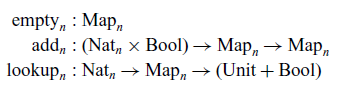
Invoking $\mathrm{lookup}~i~map$
returns
$\mathrm{lookup}~i~map$
returns $\mathbf{inl}~{\langle \rangle}$
if i is not present in map, and
$\mathbf{inl}~{\langle \rangle}$
if i is not present in map, and $\mathbf{inr}~ans$
if i is associated by map with the value
$\mathbf{inr}~ans$
if i is associated by map with the value $ans : \mathrm{Bool}$
. Allowing ourselves a few extra constant-time arithmetic operations, we can realise suitable maps in
$ans : \mathrm{Bool}$
. Allowing ourselves a few extra constant-time arithmetic operations, we can realise suitable maps in ${\lambda_{\textrm{b}}}$
such that the time complexity of
${\lambda_{\textrm{b}}}$
such that the time complexity of $\mathrm{add}_n$
and
$\mathrm{add}_n$
and $\mathrm{lookup}_n$
is
$\mathrm{lookup}_n$
is ${{{{{{\mathcal{O}}}}}}}(\log n)$
(Okasaki, Reference Okasaki1999). We can then use parameter-passing to support repeated queries as follows.
${{{{{{\mathcal{O}}}}}}}(\log n)$
(Okasaki, Reference Okasaki1999). We can then use parameter-passing to support repeated queries as follows.

The state parameter s memoises query results, thus avoiding double-counting and enabling $\mathrm{effcount}'_n$
to work correctly for predicates performing the same query multiple times.
$\mathrm{effcount}'_n$
to work correctly for predicates performing the same query multiple times.
Missing queries. Similarly, we can use parameter-passing to support missing queries.

The parameter d tracks the depth and the returned result is scaled by $2^{n-d}$
accounting for the unexplored part of the current subtree. This enables
$2^{n-d}$
accounting for the unexplored part of the current subtree. This enables $\mathrm{effcount}''_n$
to operate correctly on predicates that inspect n points at most once. We leave it as an exercise for the reader to combine
$\mathrm{effcount}''_n$
to operate correctly on predicates that inspect n points at most once. We leave it as an exercise for the reader to combine $\mathrm{effcount}'_n$
and
$\mathrm{effcount}'_n$
and $\mathrm{effcount}''_n$
to handle both repeated queries and missing queries.
$\mathrm{effcount}''_n$
to handle both repeated queries and missing queries.
6.2 From generic count to generic search
We can generalise the problem of generic counting to generic searching. The key difference is that a generic search procedure must materialise a list of solutions, thus its type is
 \[ \mathrm{search}_{n} : ((\mathrm{Nat}_n \to \mathrm{Bool}) \to \mathrm{Bool}) \to \mathrm{List}_{\mathrm{Nat}_n \to \mathrm{Bool}}\]
where $\mathrm{List}_A$
is the type of cons-lists whose elements have type A. We modify effcount to return a list of solutions rather than the number of solutions by lifting each result into a singleton list and using list concatenation instead of addition to combine partial results
$\mathrm{List}_A$
is the type of cons-lists whose elements have type A. We modify effcount to return a list of solutions rather than the number of solutions by lifting each result into a singleton list and using list concatenation instead of addition to combine partial results $xs_\mathrm{true}$
and
$xs_\mathrm{true}$
and $xs_\mathrm{false}$
as follows.
$xs_\mathrm{false}$
as follows.

The Branch operation is now parameterised by an index i. The handler is now parameterised by the current path as a point q, which is output at a leaf if it is in the predicate. A little care is required to ensure that $\text{effSearch}_\textit{n}$
has runtime
$\text{effSearch}_\textit{n}$
has runtime ${{{{{{\mathcal{O}}}}}}}(2^n)$
; naïve use of cons-list concatenation would result in
${{{{{{\mathcal{O}}}}}}}(2^n)$
; naïve use of cons-list concatenation would result in ${{{{{{\mathcal{O}}}}}}}(n2^n)$
runtime, as cons-list concatenation is linear in its first operand. In place of cons-lists, we use Hughes lists (Hughes, Reference Hughes1986), which admit constant time concatenation:
${{{{{{\mathcal{O}}}}}}}(n2^n)$
runtime, as cons-list concatenation is linear in its first operand. In place of cons-lists, we use Hughes lists (Hughes, Reference Hughes1986), which admit constant time concatenation: $\text{HList}_A \mathrel{\overset{{\mbox{def}}}{=}} \mathrm{List}_A \to \mathrm{List}_A$
. The empty Hughes list
$\text{HList}_A \mathrel{\overset{{\mbox{def}}}{=}} \mathrm{List}_A \to \mathrm{List}_A$
. The empty Hughes list $\mathrm{nil} : \text{HList}_A$
is defined as the identity function:
$\mathrm{nil} : \text{HList}_A$
is defined as the identity function: $\mathrm{nil} \mathrel{\overset{{\mbox{def}}}{=}} \lambda xs. xs$
.
$\mathrm{nil} \mathrel{\overset{{\mbox{def}}}{=}} \lambda xs. xs$
.

We use the function $\text{toConsList}$
to convert the final Hughes list to a standard cons-list. This conversion has linear time complexity (it just conses all of the elements of the list together).
$\text{toConsList}$
to convert the final Hughes list to a standard cons-list. This conversion has linear time complexity (it just conses all of the elements of the list together).
6.3 Type-and-effect system
Many practical implementations of effect handlers come equipped with rich type systems that track which effectful operations any function may perform (Bauer & Pretnar, Reference Bauer and Pretnar2014; Hillerström & Lindley, Reference Hillerström and Lindley2016; Leijen, Reference Leijen2017; Biernacki et al., Reference Biernacki, Piróg, Polesiuk and Sieczkowski2019; Brachthäuser et al., Reference Brachthäuser, Schuster and Ostermann2020). One may wonder whether our result transfers to such a system as we make crucial use of the ability to inject an effectful operation into a computation, which a first glance might seem to require a change of (effect) types.
However, as we shall briefly outline, with sufficient polymorphism we need not change the effect types. Our generic count program does not perform any externally visible effects. Therefore, if we equip our simple type system with some form of rank-2 effect polymorphism, then we do not morally require a change of types even in the presence of the richer types provided by effect tracking.
Suppose we track the effects on function types, e.g. $A \to B !\varepsilon$
denotes a function that accepts a value of type A as input and produces some value of type B as output using effects
$A \to B !\varepsilon$
denotes a function that accepts a value of type A as input and produces some value of type B as output using effects $\varepsilon$
. Here
$\varepsilon$
. Here $\varepsilon$
is intended to be an effect variable which may be instantiated to name concrete effectful operations that the function may perform such as
$\varepsilon$
is intended to be an effect variable which may be instantiated to name concrete effectful operations that the function may perform such as $\mathrm{Branch} : \mathrm{Unit} \to \mathrm{Bool}$
. We shall not concern ourselves with a particular effect type formalism here, but rather just note that there are many approaches to realising such an effect system, e.g. using row types (Hillerström & Lindley, Reference Hillerström and Lindley2016; Leijen, Reference Leijen2017), subtyping (Bauer & Pretnar, Reference Bauer and Pretnar2014), intersection types (Brachthäuser et al., Reference Brachthäuser, Schuster and Ostermann2020), etc.
$\mathrm{Branch} : \mathrm{Unit} \to \mathrm{Bool}$
. We shall not concern ourselves with a particular effect type formalism here, but rather just note that there are many approaches to realising such an effect system, e.g. using row types (Hillerström & Lindley, Reference Hillerström and Lindley2016; Leijen, Reference Leijen2017), subtyping (Bauer & Pretnar, Reference Bauer and Pretnar2014), intersection types (Brachthäuser et al., Reference Brachthäuser, Schuster and Ostermann2020), etc.
We can give a fully effect-parametric signature to generic count using rank-2 effect polymorphism.
 \[ \mathrm{Count} : (\forall \varepsilon. (\mathrm{Nat} \to \mathrm{Bool} ! \varepsilon) \to \mathrm{Bool} ! \varepsilon) \to \mathrm{Nat} ! \emptyset\]
Here $\emptyset$
denotes that an application of Count does not perform any externally visible effects. The parameter type of Count is a rank-2 effect type. It effectively hides the implementation detail of the provided point from the predicate. Thus, the implementation of Count is allowed to supply a point that performs any effectful operation granted that the implementation guarantees to handle any such operation. This idea of using rank-2 polymorphism is an old idea which dates back at least to McCracken (Reference McCracken1984); it has been used in practice in Haskell as the primary means for state encapsulation since Launchbury & Jones (Reference Launchbury and Jones1994).
$\emptyset$
denotes that an application of Count does not perform any externally visible effects. The parameter type of Count is a rank-2 effect type. It effectively hides the implementation detail of the provided point from the predicate. Thus, the implementation of Count is allowed to supply a point that performs any effectful operation granted that the implementation guarantees to handle any such operation. This idea of using rank-2 polymorphism is an old idea which dates back at least to McCracken (Reference McCracken1984); it has been used in practice in Haskell as the primary means for state encapsulation since Launchbury & Jones (Reference Launchbury and Jones1994).
7 Generic count in weaker languages
We have shown that there is an implementation of generic count in ${\lambda_{\textrm{h}}}$
with a runtime bound of
${\lambda_{\textrm{h}}}$
with a runtime bound of ${{{{{{\mathcal{O}}}}}}}(2^n)$
for certain well-behaved predicates. Our eventual goal is to prove that such a runtime bound is unattainable in
${{{{{{\mathcal{O}}}}}}}(2^n)$
for certain well-behaved predicates. Our eventual goal is to prove that such a runtime bound is unattainable in ${\lambda_{\textrm{b}}}$
(Section 8), or indeed in the stronger language
${\lambda_{\textrm{b}}}$
(Section 8), or indeed in the stronger language ${{{{{{\lambda_{\textrm{a}}}}}}}}$
(Section 10). In this section, we provide some context for these results by surveying a range of possible approaches to generic counting in languages weaker than
${{{{{{\lambda_{\textrm{a}}}}}}}}$
(Section 10). In this section, we provide some context for these results by surveying a range of possible approaches to generic counting in languages weaker than ${\lambda_{\textrm{h}}}$
, emphasising how the attainable efficiency varies according to the expressivity of the language. Since the purpose here is simply to situate our main results within a broader landscape which may itself call for further investigation, our discussion in this section will be informal and intuitive rather than mathematically rigorous.
${\lambda_{\textrm{h}}}$
, emphasising how the attainable efficiency varies according to the expressivity of the language. Since the purpose here is simply to situate our main results within a broader landscape which may itself call for further investigation, our discussion in this section will be informal and intuitive rather than mathematically rigorous.
7.1 Naïve count
The naïve approach, of course, is simply to apply the given predicate P to all $2^n$
possible n-points in turn, keeping a count of those on which P yields true. Of course, this approach could be readily implemented in
$2^n$
possible n-points in turn, keeping a count of those on which P yields true. Of course, this approach could be readily implemented in ${\lambda_{\textrm{b}}}$
; but it is also clear how it could be effected in an even weaker language, in which the recursion construct of
${\lambda_{\textrm{b}}}$
; but it is also clear how it could be effected in an even weaker language, in which the recursion construct of ${\lambda_{\textrm{b}}}$
is replaced by a weaker iteration construct. (For a comparison of the power of iteration and recursion, see Longley, Reference Longley2019.) For instance, the following operator (definable in
${\lambda_{\textrm{b}}}$
is replaced by a weaker iteration construct. (For a comparison of the power of iteration and recursion, see Longley, Reference Longley2019.) For instance, the following operator (definable in ${\lambda_{\textrm{b}}}$
) allows one to achieve the effect of while-loops manipulating data of type A:
${\lambda_{\textrm{b}}}$
) allows one to achieve the effect of while-loops manipulating data of type A:

Let us write ${{{{{{\lambda_{\textrm{i}}}}}}}}$
for the sublanguage of
${{{{{{\lambda_{\textrm{i}}}}}}}}$
for the sublanguage of ${\lambda_{\textrm{b}}}$
allowing
${\lambda_{\textrm{b}}}$
allowing $\mathrm{while}_A$
for each type A, but disallowing all uses of
$\mathrm{while}_A$
for each type A, but disallowing all uses of $\mathbf{rec}$
elsewhere. Then it is a straightforward coding exercise to write a
$\mathbf{rec}$
elsewhere. Then it is a straightforward coding exercise to write a ${{{{{{\lambda_{\textrm{i}}}}}}}}$
program
${{{{{{\lambda_{\textrm{i}}}}}}}}$
program
 \[ {\mathrm{naivecount}}_n ~: ((\mathrm{Nat}_n \to \mathrm{Bool}) \to \mathrm{Bool}) \to \mathrm{Nat} \]
that implements generic counting using the naïve strategy.
The evaluation of an n-standard predicate on an individual n-point must clearly take time $\Omega(n)$
. It is therefore clear that in whatever way the naïve count strategy is implemented, the runtime on any n-standard predicate P must be
$\Omega(n)$
. It is therefore clear that in whatever way the naïve count strategy is implemented, the runtime on any n-standard predicate P must be $\Omega(n2^n)$
. If P is not n-standard, the
$\Omega(n2^n)$
. If P is not n-standard, the $\Omega(n)$
bound on each point application need not apply, but we may still say that a naïve count for any predicate P (at level n) must take time
$\Omega(n)$
bound on each point application need not apply, but we may still say that a naïve count for any predicate P (at level n) must take time $\Omega(2^n)$
.
$\Omega(2^n)$
.
One might at first suppose that these properties are inevitable for any implementation of generic count within ${\lambda_{\textrm{b}}}$
, or indeed any purely functional language: surely, the only way to learn something about the behaviour of P on every possible n-point is to apply P to each of these points in turn? It turns out, however, that the
${\lambda_{\textrm{b}}}$
, or indeed any purely functional language: surely, the only way to learn something about the behaviour of P on every possible n-point is to apply P to each of these points in turn? It turns out, however, that the $\Omega(2^n)$
lower bound can sometimes be circumvented by implementations that cleverly exploit nesting of calls to P. In the next section, we illustrate the germ of this idea, and in Section 7.3, we show how it gives rise to a practically superior counting program within
$\Omega(2^n)$
lower bound can sometimes be circumvented by implementations that cleverly exploit nesting of calls to P. In the next section, we illustrate the germ of this idea, and in Section 7.3, we show how it gives rise to a practically superior counting program within ${\lambda_{\textrm{b}}}$
.
${\lambda_{\textrm{b}}}$
.
7.2 The nesting trick
The germ of the idea may be illustrated even within ${{{{{{\lambda_{\textrm{i}}}}}}}}$
. Suppose that we first construct some program
${{{{{{\lambda_{\textrm{i}}}}}}}}$
. Suppose that we first construct some program
 \[ {\mathrm{bestshot}}_n ~: ((\mathrm{Nat}_n \to \mathrm{Bool}) \to \mathrm{Bool}) \to (\mathrm{Nat}_n \to \mathrm{Bool})\]
which, given a predicate P, returns some n-point Q such that $P~Q$
evaluates to true, if such a point exists, and any point at all if no such point exists. (In other words,
$P~Q$
evaluates to true, if such a point exists, and any point at all if no such point exists. (In other words, ${\mathrm{bestshot}}_n$
embodies Hilbert’s choice operator
${\mathrm{bestshot}}_n$
embodies Hilbert’s choice operator $\varepsilon$
on predicates.) It is once again routine to construct such a program by naïve means, and we may moreover assume that for any P, the evaluation of
$\varepsilon$
on predicates.) It is once again routine to construct such a program by naïve means, and we may moreover assume that for any P, the evaluation of ${\mathrm{bestshot}}_n\;P$
takes only constant time, all the real work being deferred until the argument of type
${\mathrm{bestshot}}_n\;P$
takes only constant time, all the real work being deferred until the argument of type $\mathrm{Nat}_n$
is supplied.
$\mathrm{Nat}_n$
is supplied.
Now consider the following program:

Here the term $pred~({\mathrm{bestshot}}_n~pred)$
serves to test whether there exists an n-point satisfying pred: if there is not, our count program may return 0 straightaway. It is thus clear that
$pred~({\mathrm{bestshot}}_n~pred)$
serves to test whether there exists an n-point satisfying pred: if there is not, our count program may return 0 straightaway. It is thus clear that ${\mathrm{lazycount}}_n$
is a correct implementation of generic count, and also that if pred is the predicate
${\mathrm{lazycount}}_n$
is a correct implementation of generic count, and also that if pred is the predicate $\lambda q.\mathrm{false}$
then
$\lambda q.\mathrm{false}$
then ${\mathrm{lazycount}}_n\;pred$
returns 0 within
${\mathrm{lazycount}}_n\;pred$
returns 0 within ${{{{{{\mathcal{O}}}}}}}(1)$
time, thus violating the
${{{{{{\mathcal{O}}}}}}}(1)$
time, thus violating the $\Omega(2^n)$
lower bound suggested above.
$\Omega(2^n)$
lower bound suggested above.
This might seem like a footling point, as ${\mathrm{lazycount}}_n$
offers this efficiency gain only on (certain implementations of) the constantly false predicate. However, it turns out that by a recursive application of this nesting trick, we may arrive at a generic count program in
${\mathrm{lazycount}}_n$
offers this efficiency gain only on (certain implementations of) the constantly false predicate. However, it turns out that by a recursive application of this nesting trick, we may arrive at a generic count program in ${\lambda_{\textrm{b}}}$
that spectacularly defies the
${\lambda_{\textrm{b}}}$
that spectacularly defies the $\Omega(2^n)$
lower bound for an interesting class of (non-n-standard) predicates, and indeed proves quite viable for counting solutions to ‘n-queens’ and similar problems. In contrast to the naïve strategy, however, this approach relies crucially on the use of recursion and cannot be implemented in a language such as
$\Omega(2^n)$
lower bound for an interesting class of (non-n-standard) predicates, and indeed proves quite viable for counting solutions to ‘n-queens’ and similar problems. In contrast to the naïve strategy, however, this approach relies crucially on the use of recursion and cannot be implemented in a language such as ${{{{{{\lambda_{\textrm{i}}}}}}}}$
with mere iteration.
${{{{{{\lambda_{\textrm{i}}}}}}}}$
with mere iteration.
We shall refer to this ${\lambda_{\textrm{b}}}$
program as
${\lambda_{\textrm{b}}}$
program as ${\mathrm{Bergercount}}$
, as it is modelled largely on Berger’s PCF implementation of the so-called fan functional (Berger, Reference Berger1990; Longley & Normann, Reference Longley and Normann2015). We give an implementation of
${\mathrm{Bergercount}}$
, as it is modelled largely on Berger’s PCF implementation of the so-called fan functional (Berger, Reference Berger1990; Longley & Normann, Reference Longley and Normann2015). We give an implementation of ${\mathrm{Bergercount}}$
in the next section.
${\mathrm{Bergercount}}$
in the next section.
7.3 Berger count
Berger’s original program (Berger, Reference Berger1990) introduced a remarkable search operator for predicates on infinite streams of booleans and has played an important role in higher-order computability theory (Longley & Normann, Reference Longley and Normann2015). What we wish to highlight here is that if one applies the algorithm to predicates on finite boolean vectors, the resulting program, though no longer interesting from a computability perspective, still holds some interest from a complexity standpoint: indeed, it yields what seems to be the best known implementation of generic count within a PCF-style ‘functional’ language (provided one accepts the use of a primitive for call-by-need evaluation).
We give the gist of an adaptation of Berger’s search algorithm on finite spaces. The key ingredient of Berger’s search algorithm is the ${\mathrm{bestshot}}_n$
function, which given any n-standard predicate P returns a point satisfying P if one exists, or the dummy point
${\mathrm{bestshot}}_n$
function, which given any n-standard predicate P returns a point satisfying P if one exists, or the dummy point $\lambda i.\mathrm{false}$
if not. Figure 7 depicts the implementation of this function. It is implemented by via two mutually recursive auxiliary functions whose workings are admittedly hard to elucidate in a few words. The function
$\lambda i.\mathrm{false}$
if not. Figure 7 depicts the implementation of this function. It is implemented by via two mutually recursive auxiliary functions whose workings are admittedly hard to elucidate in a few words. The function ${\mathrm{bestshot}}'_n$
is a generalisation of
${\mathrm{bestshot}}'_n$
is a generalisation of ${\mathrm{bestshot}}_n$
that makes a best shot at finding a point
${\mathrm{bestshot}}_n$
that makes a best shot at finding a point $\pi$
satisfying given predicate and matching some specified list start in some initial segment of its components
$\pi$
satisfying given predicate and matching some specified list start in some initial segment of its components $[\pi(0),\dots,\pi(i-1)]$
. Here we use two customary operations on lists: we write
$[\pi(0),\dots,\pi(i-1)]$
. Here we use two customary operations on lists: we write $|-|$
for the list length function and nth for the function which projects the nth element of a list. The
$|-|$
for the list length function and nth for the function which projects the nth element of a list. The ${\mathrm{bestshot}}'_n$
function works ‘lazily’, drawing its values from start wherever possible, and performing an actual search only when required. This actual search is undertaken by
${\mathrm{bestshot}}'_n$
function works ‘lazily’, drawing its values from start wherever possible, and performing an actual search only when required. This actual search is undertaken by ${\mathrm{bestshot}}''_n$
, which proceeds by first searching for a solution that extends the specified list with true (using the standard list append function); but if no such solution is forthcoming, it settles for false as the next component of the point being constructed. The whole procedure relies on a subtle combination of laziness, recursion and implicit nesting of calls to the provided predicate which means that the search is self-pruning in regions of the binary tree where the predicate only demands some initial segment
${\mathrm{bestshot}}''_n$
, which proceeds by first searching for a solution that extends the specified list with true (using the standard list append function); but if no such solution is forthcoming, it settles for false as the next component of the point being constructed. The whole procedure relies on a subtle combination of laziness, recursion and implicit nesting of calls to the provided predicate which means that the search is self-pruning in regions of the binary tree where the predicate only demands some initial segment $q~0$
,
$q~0$
, $q~(i-1)$
of its argument q.
$q~(i-1)$
of its argument q.

Fig. 7. An implementation of ${\mathrm{bestshot}}$
in
${\mathrm{bestshot}}$
in ${\lambda_{\textrm{b}}}$
with memoisation.
${\lambda_{\textrm{b}}}$
with memoisation.
The above program makes use of an operation
 \[ \mathrm{memoise} : (\mathrm{Unit} \to \mathrm{List}~\mathrm{Bool}) \to (\mathrm{Unit} \to \mathrm{List}~\mathrm{Bool})\]
which transforms a given thunk into an equivalent ‘memoised’ version, i.e. one that caches its value after its first invocation and immediately returns this value on all subsequent invocations. Such an operation may readily be implemented with the help of local state, or alternatively may simply be added as a primitive in its own right. The latter has the advantage that it preserves the purely ‘functional’ character of the language, in the sense that every program is observationally equivalent to a ${\lambda_{\textrm{b}}}$
program, namely the one obtained by replacing memoise by the identity.
${\lambda_{\textrm{b}}}$
program, namely the one obtained by replacing memoise by the identity.
Figure 8 depicts an implementation that exploits the above idea to yield a generic count program (this development appears to be new). Again, ${\mathrm{Bergercount}}_n$
is implemented by means of two mutually recursive auxiliary functions. The function
${\mathrm{Bergercount}}_n$
is implemented by means of two mutually recursive auxiliary functions. The function $\mathrm{count}'_n$
counts the solutions to the provided predicate pred that start with the specified list of booleans, adding their number to a previously accumulated total given by acc. The function
$\mathrm{count}'_n$
counts the solutions to the provided predicate pred that start with the specified list of booleans, adding their number to a previously accumulated total given by acc. The function $\mathrm{count}''_n$
does the same thing, but exploiting the knowledge that a best shot at the ‘leftmost’ solution to P within this subtree has already been computed. (We are visualising n-points as forming a binary tree with true to the left of false at each fork.) Thus,
$\mathrm{count}''_n$
does the same thing, but exploiting the knowledge that a best shot at the ‘leftmost’ solution to P within this subtree has already been computed. (We are visualising n-points as forming a binary tree with true to the left of false at each fork.) Thus, $\mathrm{count}''_n$
will not re-examine the portion of the subtree to the left of this candidate solution, but rather will start at this solution and work rightward.
$\mathrm{count}''_n$
will not re-examine the portion of the subtree to the left of this candidate solution, but rather will start at this solution and work rightward.

Fig. 8. An implementation of Berger count in ${\lambda_{\textrm{b}}}$
.
${\lambda_{\textrm{b}}}$
.
This gives rise to an n-count program that can work efficiently on predicates that tend to ‘fail fast’: more specifically, predicates P that inspect the components of their argument q in order $q~0$
,
$q~0$
, $q~1$
,
$q~1$
, $q~2$
, and which are frequently able to return false after inspecting just a small number of these components. Generalising our program from binary to k-ary branching trees, we see that the n-queens problem provides a typical example: most points in the space can be seen not to be solutions by inspecting just the first few components. Our experimental results in Section 11 attest to the viability of this approach and its overwhelming superiority over the naïve functional method.
$q~2$
, and which are frequently able to return false after inspecting just a small number of these components. Generalising our program from binary to k-ary branching trees, we see that the n-queens problem provides a typical example: most points in the space can be seen not to be solutions by inspecting just the first few components. Our experimental results in Section 11 attest to the viability of this approach and its overwhelming superiority over the naïve functional method.
By contrast, the above program is not able to exploit parts of the tree where our predicate ‘succeeds fast’, i.e. returns true after seeing just a few components. Unlike the effectful count program of Section 5.4, which may sometimes add $2^{n-d}$
to the count in a single step, the Berger approach can only count solutions one at a time. Thus, for an n-standard predicate P, the evaluation of
$2^{n-d}$
to the count in a single step, the Berger approach can only count solutions one at a time. Thus, for an n-standard predicate P, the evaluation of ${\mathrm{Bergercount}}_n~P$
that returns a natural number k must take time
${\mathrm{Bergercount}}_n~P$
that returns a natural number k must take time $\Omega(k)$
.
$\Omega(k)$
.
7.4 Pruned count
To do better than ${\mathrm{Bergercount}}$
, it seems that we must ascend to a more powerful language. We now briefly outline another approach, using ideas from Longley (Reference Longley1999), which yields a more efficient form of pruned search in an extension of
${\mathrm{Bergercount}}$
, it seems that we must ascend to a more powerful language. We now briefly outline another approach, using ideas from Longley (Reference Longley1999), which yields a more efficient form of pruned search in an extension of $\lambda_b$
with local state of ground type. Since local state can certainly be encoded using affine effect handlers with no essential loss of efficiency, this approach falls within the ambit of what can be achieved within the language
$\lambda_b$
with local state of ground type. Since local state can certainly be encoded using affine effect handlers with no essential loss of efficiency, this approach falls within the ambit of what can be achieved within the language ${{{{{{\lambda_{\textrm{a}}}}}}}}$
to be introduced in Section 9.
${{{{{{\lambda_{\textrm{a}}}}}}}}$
to be introduced in Section 9.
The key idea is that each time we apply a predicate to a point, we may use local state to detect which components of the point are actually inspected by the predicate. We do this using a third-order function Modulus, which encloses the point in a wrapper that logs all calls to the point, then passes this wrapped point to the predicate:

This is somewhat different from the modulus functional considered in Longley (Reference Longley1999), which returns a sorted list of the arguments to which the point is applied. The latter has the theoretically pleasant consequence that the modulus is an example of a sequentially realisable functional – its externally observable behaviour is purely functional (i.e. extensional) although the function it implements cannot be realised in pure $\lambda_b$
. However, this property is purchased at the cost of the extra work needed to return a sorted list and is of little relevance to our present concerns.
$\lambda_b$
. However, this property is purchased at the cost of the extra work needed to return a sorted list and is of little relevance to our present concerns.
The essential point is that if $\mathrm{Modulus}~pred~point$
returns
$\mathrm{Modulus}~pred~point$
returns ${{{{{{\langle b,ilist \rangle}}}}}}$
, then we know immediately that
${{{{{{\langle b,ilist \rangle}}}}}}$
, then we know immediately that $pred~point'$
would also return the value b for every point’ that agrees with point at the components listed in ilist. This property can be used as the basis of a program
$pred~point'$
would also return the value b for every point’ that agrees with point at the components listed in ilist. This property can be used as the basis of a program
 \[ {\mathrm{prunedcount}}_n ~: ((\mathrm{Nat}_n \to \mathrm{Bool}) \to \mathrm{Bool}) \to \mathrm{Nat} \]
that takes care, at each stage, to apply the predicate to some ‘new’ point at which the value is not already known on the basis of previous calls, and which then increments the accumulator by either 0 (if the predicate returns false) or the appropriate $2^{n-d}$
(if it returns true). In contrast to
$2^{n-d}$
(if it returns true). In contrast to ${\mathrm{Bergercount}}$
, this has the effect of pruning the search space both where the predicate fails fast and where it succeeds fast.
${\mathrm{Bergercount}}$
, this has the effect of pruning the search space both where the predicate fails fast and where it succeeds fast.
Of course, the ability to prune in the ‘true’ case makes no difference for search problems such as n-queens, where the predicate never returns true without inspecting all components. Even for searches of this kind, however, ${\mathrm{prunedcount}}$
performs significantly better in practice than
${\mathrm{prunedcount}}$
performs significantly better in practice than ${\mathrm{Bergercount}}$
, which achieves its pruning of ‘false’ subtrees by much more convoluted means. (The difference is clearly manifested by the experimental results reported in Section 11.) Indeed, in the absence of advanced control features, we are not aware of any approach to generic counting that essentially does better than
${\mathrm{Bergercount}}$
, which achieves its pruning of ‘false’ subtrees by much more convoluted means. (The difference is clearly manifested by the experimental results reported in Section 11.) Indeed, in the absence of advanced control features, we are not aware of any approach to generic counting that essentially does better than ${\mathrm{prunedcount}}$
.
${\mathrm{prunedcount}}$
.
It is clear, however, that in the case of n-standard predicates, which always inspect all n components of their points, no pruning at all is possible, and neither ${\mathrm{Bergercount}}$
nor
${\mathrm{Bergercount}}$
nor ${\mathrm{prunedcount}}$
improves on the
${\mathrm{prunedcount}}$
improves on the $\Omega(n2^n)$
runtime of
$\Omega(n2^n)$
runtime of ${\mathrm{naivecount}}$
.
${\mathrm{naivecount}}$
.
8 A lower bound for
${\lambda_{\textrm{b}}}$

The above discussion strongly suggests that the ${{{{{{\mathcal{O}}}}}}}(2^n)$
runtime of our
${{{{{{\mathcal{O}}}}}}}(2^n)$
runtime of our ${\lambda_{\textrm{h}}}$
generic count implementation is unattainable in
${\lambda_{\textrm{h}}}$
generic count implementation is unattainable in ${\lambda_{\textrm{b}}}$
, but also points out the existence of phenomena in this area that defy intuition (Escardó, Reference Escardó2007 gives some striking further examples). In this section, we prove rigorously that any implementation of generic counting in
${\lambda_{\textrm{b}}}$
, but also points out the existence of phenomena in this area that defy intuition (Escardó, Reference Escardó2007 gives some striking further examples). In this section, we prove rigorously that any implementation of generic counting in ${\lambda_{\textrm{b}}}$
must have runtime
${\lambda_{\textrm{b}}}$
must have runtime $\Omega(n2^n)$
on certain n-standard predicates. In the following two sections, we shall apply a similar analysis to the richer language
$\Omega(n2^n)$
on certain n-standard predicates. In the following two sections, we shall apply a similar analysis to the richer language ${{{{{{\lambda_{\textrm{a}}}}}}}}$
. This mathematically robust characterisation of the efficiency gap between languages with and without first-class control constructs is the central contribution of the paper.
${{{{{{\lambda_{\textrm{a}}}}}}}}$
. This mathematically robust characterisation of the efficiency gap between languages with and without first-class control constructs is the central contribution of the paper.
One might ask at this point whether the claimed lower bound could not be obviated by means of some known continuation passing style (CPS) or monadic transform of effect handlers (Hillerström et al., Reference Hillerström, Lindley, Atkey and Sivaramakrishnan2017; Leijen, Reference Leijen2017; Hillerström et al., Reference Hillerström, Lindley and Longley2020). This can indeed be done, but only by dint of changing the type of our predicates P – which, as noted in the introduction, would defeat the purpose of our enquiry. Our intention is precisely to investigate the relative power of various languages for manipulating predicates that are given to us in a certain way which we do not have the luxury of choosing.
As a first step, we note that where lower bounds are concerned, it will suffice to work with the small-step operational semantics of ${\lambda_{\textrm{b}}}$
rather than the more elaborate abstract machine model employed in Section 4.1. This is because, as observed in Section 4.1, there is a tight correspondence between these two execution models such that for the evaluation of any closed term, the number of abstract machine steps is always at least the number of small-step reductions. Thus, if we are able to show that the number of small-step reductions for any generic count program in
${\lambda_{\textrm{b}}}$
rather than the more elaborate abstract machine model employed in Section 4.1. This is because, as observed in Section 4.1, there is a tight correspondence between these two execution models such that for the evaluation of any closed term, the number of abstract machine steps is always at least the number of small-step reductions. Thus, if we are able to show that the number of small-step reductions for any generic count program in ${\lambda_{\textrm{b}}}$
on the predicates of interest is
${\lambda_{\textrm{b}}}$
on the predicates of interest is $\Omega(n2^n)$
, this will establish the desired lower bound on the runtime.
$\Omega(n2^n)$
, this will establish the desired lower bound on the runtime.
To establish a formal contrast with ${\lambda_{\textrm{h}}}$
, it will in fact suffice to show a lower bound of
${\lambda_{\textrm{h}}}$
, it will in fact suffice to show a lower bound of $\Omega(n2^n)$
on the worst-case runtime for generic count programs in
$\Omega(n2^n)$
on the worst-case runtime for generic count programs in ${\lambda_{\textrm{b}}}$
. For this purpose, it is convenient to focus on a specialised class of predicate terms that will be easy to work with. We therefore declare that our intention is initially to analyse the runtime of any generic count program in
${\lambda_{\textrm{b}}}$
. For this purpose, it is convenient to focus on a specialised class of predicate terms that will be easy to work with. We therefore declare that our intention is initially to analyse the runtime of any generic count program in ${\lambda_{\textrm{b}}}$
on any canonical n-standard predicate as in Definition 8. However, we shall subsequently remark that in fact the same lower bound applies to arbitrary n-standard predicates.
${\lambda_{\textrm{b}}}$
on any canonical n-standard predicate as in Definition 8. However, we shall subsequently remark that in fact the same lower bound applies to arbitrary n-standard predicates.
Let us suppose, then, that K is a program of ${\lambda_{\textrm{b}}}$
that correctly counts all canonical n-standard predicates of
${\lambda_{\textrm{b}}}$
that correctly counts all canonical n-standard predicates of ${\lambda_{\textrm{b}}}$
for some specific n. We now establish a key lemma, which vindicates the naïve intuition that if P is a canonical n-standard predicate, the only way for K to discover the correct value for
${\lambda_{\textrm{b}}}$
for some specific n. We now establish a key lemma, which vindicates the naïve intuition that if P is a canonical n-standard predicate, the only way for K to discover the correct value for $\sharp [\![ P ]\!] $
is to perform
$\sharp [\![ P ]\!] $
is to perform $2^n$
separate applications
$2^n$
separate applications $P\;Q$
(allowing for the possibility that these applications need not be performed ‘in turn’ but might be nested in some complex way).
$P\;Q$
(allowing for the possibility that these applications need not be performed ‘in turn’ but might be nested in some complex way).
Lemma 1 (No shortcuts). Suppose K correctly counts all canonical n-standard predicates of ${\lambda_{\textrm{b}}}$
. If P is a canonical n-standard predicate, then K applies P to at least
${\lambda_{\textrm{b}}}$
. If P is a canonical n-standard predicate, then K applies P to at least $2^n$
distinct n-points. More formally, for any of the
$2^n$
distinct n-points. More formally, for any of the $2^n$
possible semantic n-points
$2^n$
possible semantic n-points $\pi : {{{{{{\mathbb{N}}}}}}}_n \to {{{{{{\mathbb{B}}}}}}}$
, there is a term
$\pi : {{{{{{\mathbb{N}}}}}}}_n \to {{{{{{\mathbb{B}}}}}}}$
, there is a term ${{{{{{\mathcal{E}}}}}}}[P~Q]$
appearing in the small-step reduction of
${{{{{{\mathcal{E}}}}}}}[P~Q]$
appearing in the small-step reduction of $K~P$
such that Q is an n-point and
$K~P$
such that Q is an n-point and $[\![ Q ]\!] = \pi$
.
$[\![ Q ]\!] = \pi$
.
Proof. Suppose $\pi$
is some semantic n-point. Since P is canonical, we have
$\pi$
is some semantic n-point. Since P is canonical, we have $P = P(\tau)$
for some
$P = P(\tau)$
for some $\tau$
. Let l be the maximal path through
$\tau$
. Let l be the maximal path through $\tau$
associated with
$\tau$
associated with $\pi$
: that is, the one we construct by responding to each query
$\pi$
: that is, the one we construct by responding to each query $\mathord{?} k$
with
$\mathord{?} k$
with $\pi(k)$
. Then l is a leaf node such that
$\pi(k)$
. Then l is a leaf node such that $\tau(l) = \mathord{!} (\tau \bullet \pi)$
. Let
$\tau(l) = \mathord{!} (\tau \bullet \pi)$
. Let $\tau'$
be obtained from
$\tau'$
be obtained from $\tau$
by simply negating this answer value at l, and take
$\tau$
by simply negating this answer value at l, and take $P' = P(\tau')$
.
$P' = P(\tau')$
.
Since the numbers of true-leaves in $\tau$
and
$\tau$
and $\tau'$
differ by 1, it is clear that if K indeed correctly counts all canonical n-standard predicates, then the values returned by
$\tau'$
differ by 1, it is clear that if K indeed correctly counts all canonical n-standard predicates, then the values returned by $K~P$
and
$K~P$
and $K~P'$
will have an absolute difference of 1. On the other hand, we shall argue that if the computation of
$K~P'$
will have an absolute difference of 1. On the other hand, we shall argue that if the computation of $K~P$
never actually ‘visits’ the leaf l in question, then K will be unable to detect any difference between P and P’. The situation is reminiscent of Milner’s context lemma (Milner, Reference Milner1977), which loosely says that the only way to observe a difference between two programs is to apply them to some argument on which they differ.
$K~P$
never actually ‘visits’ the leaf l in question, then K will be unable to detect any difference between P and P’. The situation is reminiscent of Milner’s context lemma (Milner, Reference Milner1977), which loosely says that the only way to observe a difference between two programs is to apply them to some argument on which they differ.
Without loss of generality we shall assume $\tau(l) = \mathrm{true}$
and
$\tau(l) = \mathrm{true}$
and $\tau'(l) = \mathrm{false}$
. This means that for some term context
$\tau'(l) = \mathrm{false}$
. This means that for some term context $C[-]:\mathrm{Bool}$
with a single occurrence of a hole of type Bool, we have
$C[-]:\mathrm{Bool}$
with a single occurrence of a hole of type Bool, we have $P \equiv \lambda q.\,C[\mathrm{true}]$
and
$P \equiv \lambda q.\,C[\mathrm{true}]$
and $P' \equiv \lambda q.\,C[\mathrm{false}]$
.
$P' \equiv \lambda q.\,C[\mathrm{false}]$
.
Now consider the reduction sequence starting from $K~(\lambda q.\,C[-])$
(treating the hole ‘
$K~(\lambda q.\,C[-])$
(treating the hole ‘ $-$
’ as an additional variable). This cannot be infinite, for then the reduction of
$-$
’ as an additional variable). This cannot be infinite, for then the reduction of $K~P$
would also be infinite, since valid reduction steps are closed under substituting true for ‘
$K~P$
would also be infinite, since valid reduction steps are closed under substituting true for ‘ $-$
’; thus K would not correctly count all canonical n-standard predicates. Neither can this reduction terminate in a numeral k, for then both
$-$
’; thus K would not correctly count all canonical n-standard predicates. Neither can this reduction terminate in a numeral k, for then both $K~P$
and
$K~P$
and $K~P'$
would evaluate to k for a similar reason, whereas the correct results should differ by 1. Nor can it terminate in just the term ’
$K~P'$
would evaluate to k for a similar reason, whereas the correct results should differ by 1. Nor can it terminate in just the term ’ $-$
’, as this does not have the correct type. We conclude that the reduction of
$-$
’, as this does not have the correct type. We conclude that the reduction of $K~(\lambda q.\,C[-])$
gets stuck at some term with the hole in head position: more precisely, since ‘
$K~(\lambda q.\,C[-])$
gets stuck at some term with the hole in head position: more precisely, since ‘ $-$
’ formally has type
$-$
’ formally has type ${{{{{{\langle + \rangle}}}}}} {\langle \rangle}$
, we see by inspection of the reduction rules that it must get stuck at some term
${{{{{{\langle + \rangle}}}}}} {\langle \rangle}$
, we see by inspection of the reduction rules that it must get stuck at some term ${{{{{{\mathcal{D}}}}}}}[\mathbf{case}\;-\;\{\cdots\}]$
, where
${{{{{{\mathcal{D}}}}}}}[\mathbf{case}\;-\;\{\cdots\}]$
, where ${{{{{{\mathcal{D}}}}}}}$
is an evaluation context. We write this term as
${{{{{{\mathcal{D}}}}}}}$
is an evaluation context. We write this term as $D[-]$
, where the
$D[-]$
, where the $D[~]$
abstracts only this head occurrence of the hole (there may well be other occurrences of the hole within D). From the form of evaluation contexts, we know that this hole occurrence does not appear under a
$D[~]$
abstracts only this head occurrence of the hole (there may well be other occurrences of the hole within D). From the form of evaluation contexts, we know that this hole occurrence does not appear under a $\lambda$
binder.
$\lambda$
binder.
We now trace back through the reduction $K~(\lambda q.\,C[-]) {{{{{{\leadsto}}}}}}^\ast D[-]$
looking at the ancestors of this occurrence of ‘
$K~(\lambda q.\,C[-]) {{{{{{\leadsto}}}}}}^\ast D[-]$
looking at the ancestors of this occurrence of ‘ $-$
’, and identifying the last point in the reduction at which this ancestor occurs within a descendant of the original
$-$
’, and identifying the last point in the reduction at which this ancestor occurs within a descendant of the original $\lambda q.\,C[-]$
. Since
$\lambda q.\,C[-]$
. Since $C[-]$
has no free variables other than the hole occurrence, and the only rule for eliminating a
$C[-]$
has no free variables other than the hole occurrence, and the only rule for eliminating a $\lambda$
is S-App, it is clear that at this point we have a term
$\lambda$
is S-App, it is clear that at this point we have a term ${{{{{{\mathcal{E}}}}}}}[(\lambda q.\,C[-])Q]$
with
${{{{{{\mathcal{E}}}}}}}[(\lambda q.\,C[-])Q]$
with ${{{{{{\mathcal{E}}}}}}}$
an evaluation context,
${{{{{{\mathcal{E}}}}}}}$
an evaluation context, $C[~]$
a context abstracting only this ancestor occurrence of ‘
$C[~]$
a context abstracting only this ancestor occurrence of ‘ $-$
’, and Q a closed term of type Point. This reduces in the next step to
$-$
’, and Q a closed term of type Point. This reduces in the next step to ${{{{{{\mathcal{E}}}}}}}[E[-]]$
where
${{{{{{\mathcal{E}}}}}}}[E[-]]$
where $E[-] \equiv C[-][Q/q]$
.
$E[-] \equiv C[-][Q/q]$
.
We now claim that Q is an n-point and $[\![ Q ]\!] = \pi$
as required. For this, we appeal to the fact that
$[\![ Q ]\!] = \pi$
as required. For this, we appeal to the fact that $P \equiv \lambda q.\,C[\mathrm{true}]$
is canonical, so that
$P \equiv \lambda q.\,C[\mathrm{true}]$
is canonical, so that $C[-]$
is simply a complex of nested
$C[-]$
is simply a complex of nested $\mathbf{if}$
-expressions as in Definition 8, with a hole replacing the leaf literal at the position indicated by the path l. It follows that
$\mathbf{if}$
-expressions as in Definition 8, with a hole replacing the leaf literal at the position indicated by the path l. It follows that $E[-]$
itself is a complex of nested
$E[-]$
itself is a complex of nested $\mathbf{if}$
-expressions with branch conditions Q(k) and with the hole at one of the leaves. It is now clear that the only way for this hole to become later exposed (as it is in
$\mathbf{if}$
-expressions with branch conditions Q(k) and with the hole at one of the leaves. It is now clear that the only way for this hole to become later exposed (as it is in $D[-]$
) is for each of the branch conditions Q(k) to evaluate to
$D[-]$
) is for each of the branch conditions Q(k) to evaluate to $\pi(k)$
, so that the evaluation indeed follows the path l and we have
$\pi(k)$
, so that the evaluation indeed follows the path l and we have $E[-] {{{{{{\leadsto}}}}}}^* -$
. But because
$E[-] {{{{{{\leadsto}}}}}}^* -$
. But because $\tau$
is n-standard, each of
$\tau$
is n-standard, each of $Q(0),\ldots,Q(n-1)$
occurs exactly once on this path, so the above is exactly the condition for Q to be an n-point with value
$Q(0),\ldots,Q(n-1)$
occurs exactly once on this path, so the above is exactly the condition for Q to be an n-point with value $\pi$
.
$\pi$
.
Corollary 1. Suppose K and P are as in Lemma 1. For any semantic n-point $\pi$
and any natural number
$\pi$
and any natural number $k < n$
, the reduction sequence for
$k < n$
, the reduction sequence for $K~P$
contains a term
$K~P$
contains a term ${\mathcal{F}}[Q~k]$
, where
${\mathcal{F}}[Q~k]$
, where ${\mathcal{F}}$
is an evaluation context and
${\mathcal{F}}$
is an evaluation context and $[\![ Q ]\!] =\pi$
.
$[\![ Q ]\!] =\pi$
.
Proof Suppose $\pi \in {{{{{{\mathbb{B}}}}}}}^n$
. By Lemma 1, the computation of
$\pi \in {{{{{{\mathbb{B}}}}}}}^n$
. By Lemma 1, the computation of $K~P$
contains some
$K~P$
contains some ${{{{{{\mathcal{E}}}}}}}[P~Q]$
where
${{{{{{\mathcal{E}}}}}}}[P~Q]$
where $[\![ Q ]\!] = \pi$
, and the above analysis of the computation of
$[\![ Q ]\!] = \pi$
, and the above analysis of the computation of $P~Q$
shows that it contains a term
$P~Q$
shows that it contains a term ${{{{{{\mathcal{E}}}}}}}'[Q~k]$
for each
${{{{{{\mathcal{E}}}}}}}'[Q~k]$
for each $k < n$
. The corollary follows, taking
$k < n$
. The corollary follows, taking ${\mathcal{F}}[-] \mathrel{\overset{{\mbox{def}}}{=}} {{{{{{\mathcal{E}}}}}}}[{{{{{{\mathcal{E}}}}}}}'[-]]$
.
${\mathcal{F}}[-] \mathrel{\overset{{\mbox{def}}}{=}} {{{{{{\mathcal{E}}}}}}}[{{{{{{\mathcal{E}}}}}}}'[-]]$
.
This gives our desired lower bound. Since our n-points Q are values, it is clearly impossible that ${\mathcal{F}}[Q~k] = {\mathcal{F}}'[Q'~k']$
(where
${\mathcal{F}}[Q~k] = {\mathcal{F}}'[Q'~k']$
(where ${\mathcal{F}},{\mathcal{F}}'$
are evaluation contexts) unless
${\mathcal{F}},{\mathcal{F}}'$
are evaluation contexts) unless $Q=Q'$
and
$Q=Q'$
and $k=k'$
. We may therefore read off
$k=k'$
. We may therefore read off $\pi$
from
$\pi$
from ${\mathcal{F}}[Q~k]$
as
${\mathcal{F}}[Q~k]$
as $[\![ Q ]\!] $
. There are thus at least
$[\![ Q ]\!] $
. There are thus at least $n2^n$
distinct terms in the reduction sequence for
$n2^n$
distinct terms in the reduction sequence for $K~P$
, so the reduction has length
$K~P$
, so the reduction has length $\geq n 2^n$
. We have thus proved:
$\geq n 2^n$
. We have thus proved:
Theorem 3. If K is a ${\lambda_{\textrm{b}}}$
program that correctly counts all canonical n-standard
${\lambda_{\textrm{b}}}$
program that correctly counts all canonical n-standard ${\lambda_{\textrm{b}}}$
predicates, and P is any canonical n-standard
${\lambda_{\textrm{b}}}$
predicates, and P is any canonical n-standard ${\lambda_{\textrm{b}}}$
predicate, then the evaluation of
${\lambda_{\textrm{b}}}$
predicate, then the evaluation of $K~P$
must take time
$K~P$
must take time $\Omega(n2^n)$
.
$\Omega(n2^n)$
.
In Hillerström et al. (Reference Hillerström, Lindley and Longley2020), a more complex proof was given, modelled on traditional proofs of Milner’s context lemma. This established the slightly stronger conclusion that the evaluation of $K~P$
takes time
$K~P$
takes time $\Omega(n2^n)$
for all n-standard predicates P, not just the canonical ones (under the strengthened hypothesis that K correctly counts all n-standard
$\Omega(n2^n)$
for all n-standard predicates P, not just the canonical ones (under the strengthened hypothesis that K correctly counts all n-standard ${\lambda_{\textrm{b}}}$
predicates).
${\lambda_{\textrm{b}}}$
predicates).
It is worth noting where our argument breaks down if applied to ${\lambda_{\textrm{h}}}$
. In
${\lambda_{\textrm{h}}}$
. In ${\lambda_{\textrm{b}}}$
, in the course of computing
${\lambda_{\textrm{b}}}$
, in the course of computing $K~P$
, every Q to which P is applied will be a self-contained closed term denoting some specific point
$K~P$
, every Q to which P is applied will be a self-contained closed term denoting some specific point $\pi$
. This is intuitively why we may only learn about one point at a time. In
$\pi$
. This is intuitively why we may only learn about one point at a time. In ${\lambda_{\textrm{h}}}$
, this is not the case, because of the presence of operation symbols. For instance, our effcount program from Section 5.4 will apply P to the ‘generic point’
${\lambda_{\textrm{h}}}$
, this is not the case, because of the presence of operation symbols. For instance, our effcount program from Section 5.4 will apply P to the ‘generic point’ $\lambda\_.\,\mathbf{do}\;\mathrm{Branch}~\langle \rangle$
. Thus, it need no longer be the case that the reduction of each term
$\lambda\_.\,\mathbf{do}\;\mathrm{Branch}~\langle \rangle$
. Thus, it need no longer be the case that the reduction of each term $Q\,k$
yields a value: it may get stuck at some invocation of
$Q\,k$
yields a value: it may get stuck at some invocation of $\ell$
, so that control will then pass to the effect handler.
$\ell$
, so that control will then pass to the effect handler.
9 Affine effect handlers
Having established our $\Omega(n2^n)$
runtime bound for implementations of generic count in the relatively simple setting of
$\Omega(n2^n)$
runtime bound for implementations of generic count in the relatively simple setting of ${\lambda_{\textrm{b}}}$
, we now wish to show that the same bound applies for a much richer language
${\lambda_{\textrm{b}}}$
, we now wish to show that the same bound applies for a much richer language ${{{{{{\lambda_{\textrm{a}}}}}}}}$
supporting affine effect handlers: intuitively those in which each resumption r may be invoked at most once. This will show that the multiple invocation of r within our effcount program is essential to its efficiency, and will formally locate the fundamental efficiency gap as occurring between
${{{{{{\lambda_{\textrm{a}}}}}}}}$
supporting affine effect handlers: intuitively those in which each resumption r may be invoked at most once. This will show that the multiple invocation of r within our effcount program is essential to its efficiency, and will formally locate the fundamental efficiency gap as occurring between ${{{{{{\lambda_{\textrm{a}}}}}}}}$
and
${{{{{{\lambda_{\textrm{a}}}}}}}}$
and ${\lambda_{\textrm{h}}}$
. Since affine effect handlers suffice for encoding many language features such as exceptions (Pretnar, Reference Pretnar2015), local state (Plotkin & Pretnar, Reference Plotkin and Pretnar2009), coroutines (Kawahara & Kameyama, Reference Kawahara and Kameyama2020), and singleshot continuations (Sivaramakrishnan et al., Reference Sivaramakrishnan, Dolan, White, Kelly, Jaffer and Madhavapeddy2021), this will come close to showing that the speedup we have discussed is unattainable in real languages such as Standard ML, Java, and Python (for some appropriate class of predicate terms).
${\lambda_{\textrm{h}}}$
. Since affine effect handlers suffice for encoding many language features such as exceptions (Pretnar, Reference Pretnar2015), local state (Plotkin & Pretnar, Reference Plotkin and Pretnar2009), coroutines (Kawahara & Kameyama, Reference Kawahara and Kameyama2020), and singleshot continuations (Sivaramakrishnan et al., Reference Sivaramakrishnan, Dolan, White, Kelly, Jaffer and Madhavapeddy2021), this will come close to showing that the speedup we have discussed is unattainable in real languages such as Standard ML, Java, and Python (for some appropriate class of predicate terms).
In this section, we present the definition of our language ${{{{{{\lambda_{\textrm{a}}}}}}}}$
, outlining its relationship to
${{{{{{\lambda_{\textrm{a}}}}}}}}$
, outlining its relationship to ${\lambda_{\textrm{h}}}$
and
${\lambda_{\textrm{h}}}$
and ${\lambda_{\textrm{b}}}$
. In the following section, we will prove some key properties of evaluation in this language and use these to establish a version of Theorem 3 for
${\lambda_{\textrm{b}}}$
. In the following section, we will prove some key properties of evaluation in this language and use these to establish a version of Theorem 3 for ${{{{{{\lambda_{\textrm{a}}}}}}}}$
.
${{{{{{\lambda_{\textrm{a}}}}}}}}$
.
Our language ${{{{{{\lambda_{\textrm{a}}}}}}}}$
will be essentially a sublanguage of
${{{{{{\lambda_{\textrm{a}}}}}}}}$
will be essentially a sublanguage of ${\lambda_{\textrm{h}}}$
in which the relevant restriction on the use of resumption variables is enforced by means of an affine type system in the tradition of linear logic. Many approaches are possible here, for instance: Girard’s ntuitionistic linear logic ILL (Girard, Reference Girard1987), Barber’s dual intuitionistic linear logic DILL (Barber, Reference Barber1996), and Benton’s adjoint calculus (Benton, Reference Benton1994). We choose to work with a variant of fine-grain call-by-value based on DILL; an advantage over vanilla ILL is that it readily admits a local encoding of our intuitionistic base calculus.
${\lambda_{\textrm{h}}}$
in which the relevant restriction on the use of resumption variables is enforced by means of an affine type system in the tradition of linear logic. Many approaches are possible here, for instance: Girard’s ntuitionistic linear logic ILL (Girard, Reference Girard1987), Barber’s dual intuitionistic linear logic DILL (Barber, Reference Barber1996), and Benton’s adjoint calculus (Benton, Reference Benton1994). We choose to work with a variant of fine-grain call-by-value based on DILL; an advantage over vanilla ILL is that it readily admits a local encoding of our intuitionistic base calculus.
9.1
${{{{{{\lambda_{\textrm{a}}}}}}}}$
as a dual intuitionistic-affine calculus

We present the type system of ${{{{{{\lambda_{\textrm{a}}}}}}}}$
in terms of dual-context judgements
${{{{{{\lambda_{\textrm{a}}}}}}}}$
in terms of dual-context judgements $\Delta; \Gamma \vdash \square : A$
, stating that a term
$\Delta; \Gamma \vdash \square : A$
, stating that a term $\square$
(which may be a value term V or a computation term M) has type A under intuitionistic type environment
$\square$
(which may be a value term V or a computation term M) has type A under intuitionistic type environment $\Delta$
and affine type environment
$\Delta$
and affine type environment $\Gamma$
. Informally, variables in the intuitionistic environment may be used zero, one or many times within
$\Gamma$
. Informally, variables in the intuitionistic environment may be used zero, one or many times within $\square$
, while those in the affine environment may be used at most once.
$\square$
, while those in the affine environment may be used at most once.
As before, environments are lists assigning types to variables. For hygiene, we suppose we have disjoint lexical categories of intuitionistic and affine variables (each ranged over by metavariables x,y), and the variables within each of the environments $\Delta,\Gamma$
are required to be distinct.
$\Delta,\Gamma$
are required to be distinct.
The syntax of ${{{{{{\lambda_{\textrm{a}}}}}}}}$
is as follows:
${{{{{{\lambda_{\textrm{a}}}}}}}}$
is as follows:

The type constructors $\multimap$
,
$\multimap$
, $\otimes$
,
$\otimes$
, $\oplus$
, and
$\oplus$
, and $!$
are borrowed from linear logic. Here we informally understand Nat, Unit,
$!$
are borrowed from linear logic. Here we informally understand Nat, Unit, $A \multimap B$
,
$A \multimap B$
, $A \times B$
, and
$A \times B$
, and $A \oplus B$
as types of values that may be used at most once, and
$A \oplus B$
as types of values that may be used at most once, and $!A$
as a type of values of type A that may be used as many times as desired. (The way DILL manifests the latter is to allow a value of
$!A$
as a type of values of type A that may be used as many times as desired. (The way DILL manifests the latter is to allow a value of $!A$
to be used at most once by binding it to an intuitionistic variable of type A which can subsequently be used as many times as desired. Thus, technically
$!A$
to be used at most once by binding it to an intuitionistic variable of type A which can subsequently be used as many times as desired. Thus, technically $!A$
is affine just like all other types, but it provides access to an unlimited source of identical affine values of type A.)
$!A$
is affine just like all other types, but it provides access to an unlimited source of identical affine values of type A.)
The typing rules those shown in Figure 9, along with Exchange, Weakening and Contraction for the intuitionistic environment, and Exchange and Weakening (but not Contraction) for the affine one. To understand the workings of this type system, it is helpful to think of the affine arrow $\multimap$
and the affine environment
$\multimap$
and the affine environment $\Gamma$
as playing the primary role: for instance, lambda abstraction is supported for affine variables but not intuitionistic ones. The sole purpose of the intuitionistic environment is to allow for multiple uses of values of
$\Gamma$
as playing the primary role: for instance, lambda abstraction is supported for affine variables but not intuitionistic ones. The sole purpose of the intuitionistic environment is to allow for multiple uses of values of $!$
-type: the rule TL-LetBang allows such a value to be bound to an intuitionistic variable. Note too that values of
$!$
-type: the rule TL-LetBang allows such a value to be bound to an intuitionistic variable. Note too that values of $!$
-type are formed via the TL-Bang rule, which allows a value
$!$
-type are formed via the TL-Bang rule, which allows a value $W : A$
to be ‘promoted’ to a reusable value
$W : A$
to be ‘promoted’ to a reusable value $!W: !A$
if all free variables that went into the making of W are themselves reusable (we here write
$!W: !A$
if all free variables that went into the making of W are themselves reusable (we here write $!\Gamma$
to mean that every type in
$!\Gamma$
to mean that every type in $\Gamma$
is of the form
$\Gamma$
is of the form $!A$
for some A). Similarly, TL-BangComp allows promotion of computations. This latter form introduces some minor complications and is not strictly speaking necessary, but we include it nonetheless in order to admit a straightforward translation of let-binding in the inclusion
$!A$
for some A). Similarly, TL-BangComp allows promotion of computations. This latter form introduces some minor complications and is not strictly speaking necessary, but we include it nonetheless in order to admit a straightforward translation of let-binding in the inclusion ${{{{{{\lambda_{\textrm{b}}}}}}}}\hookrightarrow {{{{{{\lambda_{\textrm{a}}}}}}}}$
outlined at the end of this section.
${{{{{{\lambda_{\textrm{b}}}}}}}}\hookrightarrow {{{{{{\lambda_{\textrm{a}}}}}}}}$
outlined at the end of this section.

Fig. 9. Typing Rules for ${{{{{{\lambda_{\textrm{a}}}}}}}}$
The crucial restrictions in the rule for handlers are that the operation argument p and the resumption variable r are now affine. Notice that the success clause may involve affine variables as it will be invoked at most once (this idea will be substantiated in Section 10 below). By contrast, the operation clauses cannot involve affine variables as they may be invoked multiple times.
There is also a small subtlety with $\mathbf{rec}$
. The function argument f is bound in the intuitionistic type environment, allowing f to be used many times within M. The operational intention is that f can be unfolded to
$\mathbf{rec}$
. The function argument f is bound in the intuitionistic type environment, allowing f to be used many times within M. The operational intention is that f can be unfolded to $\lambda x.M$
as often as necessary; for this reason, it is required that M involves no affine variables other than x.
$\lambda x.M$
as often as necessary; for this reason, it is required that M involves no affine variables other than x.
All of the above syntactic forms are shared with ${\lambda_{\textrm{h}}}$
, with the exception of
${\lambda_{\textrm{h}}}$
, with the exception of $!W$
,
$!W$
, $!M$
, and
$!M$
, and $\mathbf{let} !\;x=V\;\mathbf{in}\;N$
. To give a small-step operational semantics for
$\mathbf{let} !\;x=V\;\mathbf{in}\;N$
. To give a small-step operational semantics for ${{{{{{\lambda_{\textrm{a}}}}}}}}$
, we may therefore take all the operational rules for
${{{{{{\lambda_{\textrm{a}}}}}}}}$
, we may therefore take all the operational rules for ${\lambda_{\textrm{h}}}$
as given in Section 3 (along with the machinery of evaluation contexts and handler contexts), together with the new rules
${\lambda_{\textrm{h}}}$
as given in Section 3 (along with the machinery of evaluation contexts and handler contexts), together with the new rules

and additional evaluation and handler contexts for promoted computations:

As usual, we take ${{{{{{\leadsto}}}}}}^*$
to be the transitive closure of
${{{{{{\leadsto}}}}}}^*$
to be the transitive closure of ${{{{{{\leadsto}}}}}}$
, and define the notions of ancestor and descendant in the evident way. This completes our definition of
${{{{{{\leadsto}}}}}}$
, and define the notions of ancestor and descendant in the evident way. This completes our definition of ${{{{{{\lambda_{\textrm{a}}}}}}}}$
.
${{{{{{\lambda_{\textrm{a}}}}}}}}$
.
The notion of normal form may now be defined just as in Definition 1. Once again, the following is straightforward to verify:
Theorem 4 (Type Soundness for ${{{{{{\lambda_{\textrm{a}}}}}}}}$
). If
${{{{{{\lambda_{\textrm{a}}}}}}}}$
). If $ \vdash M : C$
, then either there exists
$ \vdash M : C$
, then either there exists $ \vdash N : C$
such that
$ \vdash N : C$
such that $M {{{{{{\leadsto}}}}}}^\ast N$
and N is normal with respect to
$M {{{{{{\leadsto}}}}}}^\ast N$
and N is normal with respect to $\Sigma$
, or M diverges.
$\Sigma$
, or M diverges.
9.2 Relationship to
${\lambda_{\textrm{h}}}$
and
${\lambda_{\textrm{b}}}$


We now outline how we intend to view ${{{{{{\lambda_{\textrm{a}}}}}}}}$
as a sublanguage of
${{{{{{\lambda_{\textrm{a}}}}}}}}$
as a sublanguage of ${\lambda_{\textrm{h}}}$
, and
${\lambda_{\textrm{h}}}$
, and ${\lambda_{\textrm{b}}}$
as a sublanguage of
${\lambda_{\textrm{b}}}$
as a sublanguage of ${{{{{{\lambda_{\textrm{a}}}}}}}}$
. A brief sketch will suffice here, as these translations will only play a minor role in what follows and are mentioned here mainly for the sake of orientation.
${{{{{{\lambda_{\textrm{a}}}}}}}}$
. A brief sketch will suffice here, as these translations will only play a minor role in what follows and are mentioned here mainly for the sake of orientation.
For the inclusion ${{{{{{\lambda_{\textrm{a}}}}}}}} \hookrightarrow {{{{{{\lambda_{\textrm{h}}}}}}}}$
, the broad idea is simply that any well-typed term of
${{{{{{\lambda_{\textrm{a}}}}}}}} \hookrightarrow {{{{{{\lambda_{\textrm{h}}}}}}}}$
, the broad idea is simply that any well-typed term of ${{{{{{\lambda_{\textrm{a}}}}}}}}$
will certainly remain well-typed if all affineness restrictions on variables are waived. Formally, we may define a translation
${{{{{{\lambda_{\textrm{a}}}}}}}}$
will certainly remain well-typed if all affineness restrictions on variables are waived. Formally, we may define a translation ![]() that erases the intuitionistic/affine distinction completely. The translation on types may be defined by
that erases the intuitionistic/affine distinction completely. The translation on types may be defined by

The translation on terms is given in the obvious way for the syntactic forms common to ${{{{{{\lambda_{\textrm{a}}}}}}}}$
and
${{{{{{\lambda_{\textrm{a}}}}}}}}$
and ${\lambda_{\textrm{h}}}$
, the three new forms being treated by
${\lambda_{\textrm{h}}}$
, the three new forms being treated by

A typing judgement $\Delta;\Gamma \vdash \square:A$
of
$\Delta;\Gamma \vdash \square:A$
of ${{{{{{\lambda_{\textrm{a}}}}}}}}$
then becomes a judgement
${{{{{{\lambda_{\textrm{a}}}}}}}}$
then becomes a judgement ![]() , where
, where $\Delta,\Gamma$
is the result of rolling
$\Delta,\Gamma$
is the result of rolling $\Delta$
and
$\Delta$
and $\Gamma$
into a single environment, and
$\Gamma$
into a single environment, and ![]() is the result of applying
is the result of applying ![]() to the types of all its variables.
to the types of all its variables.
Under this translation, it is easy to check that every derivable typing judgement in ${{{{{{\lambda_{\textrm{a}}}}}}}}$
yields one in
${{{{{{\lambda_{\textrm{a}}}}}}}}$
yields one in ${\lambda_{\textrm{h}}}$
, and also that if
${\lambda_{\textrm{h}}}$
, and also that if $M {{{{{{\leadsto}}}}}} M'$
in
$M {{{{{{\leadsto}}}}}} M'$
in ${{{{{{\lambda_{\textrm{a}}}}}}}}$
then
${{{{{{\lambda_{\textrm{a}}}}}}}}$
then ![]() in
in ${\lambda_{\textrm{h}}}$
.
${\lambda_{\textrm{h}}}$
.
For the inclusion ${{{{{{\lambda_{\textrm{b}}}}}}}} \hookrightarrow {{{{{{\lambda_{\textrm{a}}}}}}}}$
, we give a translation
${{{{{{\lambda_{\textrm{b}}}}}}}} \hookrightarrow {{{{{{\lambda_{\textrm{a}}}}}}}}$
, we give a translation $(-)^\star$
inspired by the familiar Girard translation from intuitionistic types to linear ones, wrapping each subformula of a type by a ‘
$(-)^\star$
inspired by the familiar Girard translation from intuitionistic types to linear ones, wrapping each subformula of a type by a ‘ $!$
’ except for the return types of functions. The translation on types is as follows.
$!$
’ except for the return types of functions. The translation on types is as follows.

A type environment $\Gamma$
of
$\Gamma$
of ${\lambda_{\textrm{b}}}$
translated to the environment
${\lambda_{\textrm{b}}}$
translated to the environment $\Gamma^\star ; \cdot$
of
$\Gamma^\star ; \cdot$
of ${{{{{{\lambda_{\textrm{a}}}}}}}}$
: that is, all variables are treated as intuitionistic. The translation of value and computation terms therefore needs to eliminate ‘
${{{{{{\lambda_{\textrm{a}}}}}}}}$
: that is, all variables are treated as intuitionistic. The translation of value and computation terms therefore needs to eliminate ‘ $!$
’ types at bindings in favour of intuitionistic variables. We give here a selection of the clauses for the translation on terms; for all syntactic forms not covered here, the translation is defined homomorphically on term structure in the obvious way.
$!$
’ types at bindings in favour of intuitionistic variables. We give here a selection of the clauses for the translation on terms; for all syntactic forms not covered here, the translation is defined homomorphically on term structure in the obvious way.

Once again, it is routine to check that every derivable typing judgement in ${\lambda_{\textrm{b}}}$
yields one in
${\lambda_{\textrm{b}}}$
yields one in ${{{{{{\lambda_{\textrm{a}}}}}}}}$
, and that if
${{{{{{\lambda_{\textrm{a}}}}}}}}$
, and that if $M{{{{{{\leadsto}}}}}} M'$
in
$M{{{{{{\leadsto}}}}}} M'$
in ${\lambda_{\textrm{b}}}$
then
${\lambda_{\textrm{b}}}$
then $M^\star {{{{{{\leadsto}}}}}}^\ast {M'}^\star$
in
$M^\star {{{{{{\leadsto}}}}}}^\ast {M'}^\star$
in ${{{{{{\lambda_{\textrm{a}}}}}}}}$
.
${{{{{{\lambda_{\textrm{a}}}}}}}}$
.
10 Affine effect computations and generic count
We begin with some general machinery for managing resumptions and for tracking the evaluation of subterms through reductions, allowing for the ‘thread-switching’ behaviour that ${{{{{{\lambda_{\textrm{a}}}}}}}}$
supports. We expect that this machinery will be quite widely applicable to any kind of reasoning about the behaviour of effectful programs in
${{{{{{\lambda_{\textrm{a}}}}}}}}$
supports. We expect that this machinery will be quite widely applicable to any kind of reasoning about the behaviour of effectful programs in ${{{{{{\lambda_{\textrm{a}}}}}}}}$
. In Section 10.3, we apply this machinery to the specific scenario of the generic count problem.
${{{{{{\lambda_{\textrm{a}}}}}}}}$
. In Section 10.3, we apply this machinery to the specific scenario of the generic count problem.
Throughout this section, ‘subterm’ will always mean ‘subterm occurrence’.
10.1 Tracking of resumptions
To make the role of resumptions more explicit, it will be convenient to recast the small-step operational semantics for ${{{{{{\lambda_{\textrm{a}}}}}}}}$
slightly, presenting it as a reduction system for pairs
${{{{{{\lambda_{\textrm{a}}}}}}}}$
slightly, presenting it as a reduction system for pairs ${{{{{{\langle M \mid \Xi \rangle}}}}}}$
, where M is a term and
${{{{{{\langle M \mid \Xi \rangle}}}}}}$
, where M is a term and $\Xi$
is a resumption environment, mapping finitely many resumption variables
$\Xi$
is a resumption environment, mapping finitely many resumption variables $\hat{r}$
to terms of the form
$\hat{r}$
to terms of the form $\lambda y.\,\mathbf{handle} \; {{{{{{\mathcal{E}}}}}}}[\mathbf{return} \; y] \; \mathbf{with} \; H$
. Note that these terms may themselves involve other resumption variables.
$\lambda y.\,\mathbf{handle} \; {{{{{{\mathcal{E}}}}}}}[\mathbf{return} \; y] \; \mathbf{with} \; H$
. Note that these terms may themselves involve other resumption variables.
The only reduction rules in which $\Xi$
plays an active role are the following. We write
$\Xi$
plays an active role are the following. We write $\Xi \backslash \hat{r}$
for
$\Xi \backslash \hat{r}$
for $\Xi$
with the entry for
$\Xi$
with the entry for $\hat{r}$
deleted.
$\hat{r}$
deleted.

All other reduction rules are carried over from the original semantics in the obvious way: for each reduction rule $M {{{{{{\leadsto}}}}}} M'$
except for S-Op, we now have a rule
$M {{{{{{\leadsto}}}}}} M'$
except for S-Op, we now have a rule ${{{{{{\langle M \mid \Xi \rangle}}}}}} {{{{{{\leadsto}}}}}}{{{{{{\langle M' \mid \Xi \rangle}}}}}}$
. To initiate a reduction sequence for a closed term M, we start from the configuration
${{{{{{\langle M \mid \Xi \rangle}}}}}} {{{{{{\leadsto}}}}}}{{{{{{\langle M' \mid \Xi \rangle}}}}}}$
. To initiate a reduction sequence for a closed term M, we start from the configuration ${{{{{{\langle M \mid \emptyset \rangle}}}}}}$
.
${{{{{{\langle M \mid \emptyset \rangle}}}}}}$
.
The main purpose of this semantics is to make explicit the points at which resumptions are invoked (as the points at which S-Res is applied). In the original semantics, such steps appear simply as $\beta$
-reductions, which may not be distinguishable, on the face of it, from other
$\beta$
-reductions, which may not be distinguishable, on the face of it, from other $\beta$
-reductions that occur.
$\beta$
-reductions that occur.
It is intuitively clear that the reduction of ${{{{{{\langle M \mid \emptyset \rangle}}}}}}$
under the new semantics proceeds in lockstep with the reduction of M under the original semantics. One half of this is formalised by the following proposition (we write
${{{{{{\langle M \mid \emptyset \rangle}}}}}}$
under the new semantics proceeds in lockstep with the reduction of M under the original semantics. One half of this is formalised by the following proposition (we write ${{{{{{\leadsto}}}}}}^m$
for reduction in exactly m steps).
${{{{{{\leadsto}}}}}}^m$
for reduction in exactly m steps).
Proposition 2. For any m, if ${{{{{{\langle M \mid \emptyset \rangle}}}}}} {{{{{{\leadsto}}}}}}^m{{{{{{\langle M' \mid \Xi \rangle}}}}}}$
then
${{{{{{\langle M \mid \emptyset \rangle}}}}}} {{{{{{\leadsto}}}}}}^m{{{{{{\langle M' \mid \Xi \rangle}}}}}}$
then $M {{{{{{\leadsto}}}}}}^m M''$
, where M” is obtained from M’ by repeatedly expanding all resumption variables as specified by
$M {{{{{{\leadsto}}}}}}^m M''$
, where M” is obtained from M’ by repeatedly expanding all resumption variables as specified by $\Xi$
until no longer possible.
$\Xi$
until no longer possible.
Proof Easy induction on m. Note that in the case of $\text{S-Op}'$
, the number of rounds of expansion needed may increase by 1.
$\text{S-Op}'$
, the number of rounds of expansion needed may increase by 1.
The converse to the above proposition — that if $M {{{{{{\leadsto}}}}}}^m M''$
then
$M {{{{{{\leadsto}}}}}}^m M''$
then ${{{{{{\langle M \mid \emptyset \rangle}}}}}} {{{{{{\leadsto}}}}}}^m {{{{{{\langle M' \mid \Xi \rangle}}}}}}$
for some
${{{{{{\langle M \mid \emptyset \rangle}}}}}} {{{{{{\leadsto}}}}}}^m {{{{{{\langle M' \mid \Xi \rangle}}}}}}$
for some $M',\Xi$
— is not quite clear at this point, because of the worry that an application of S-Res might be blocked because the relevant
$M',\Xi$
— is not quite clear at this point, because of the worry that an application of S-Res might be blocked because the relevant $\hat{r}$
is not present in
$\hat{r}$
is not present in $dom\,\Xi$
, having been deleted by an earlier application of S-Res. We shall see shortly, however, that such blocking never happens, so that our two semantics do indeed work perfectly in lockstep.
$dom\,\Xi$
, having been deleted by an earlier application of S-Res. We shall see shortly, however, that such blocking never happens, so that our two semantics do indeed work perfectly in lockstep.
Let us say a configuration ${{{{{{\langle M' \mid \Xi \rangle}}}}}}$
is naturally arising if it appears in the course of reduction of
${{{{{{\langle M' \mid \Xi \rangle}}}}}}$
is naturally arising if it appears in the course of reduction of ${{{{{{\langle M \mid \emptyset \rangle}}}}}}$
for some closed M.
${{{{{{\langle M \mid \emptyset \rangle}}}}}}$
for some closed M.
In the typing rules for ${{{{{{\lambda_{\textrm{a}}}}}}}}$
, the critical typing restriction is that in the handler clauses
${{{{{{\lambda_{\textrm{a}}}}}}}}$
, the critical typing restriction is that in the handler clauses $\ell\,p\;r \mapsto N_\ell$
, the variable r is used affinely within
$\ell\,p\;r \mapsto N_\ell$
, the variable r is used affinely within $N_\ell$
. This does not mean that r can occur at most once within
$N_\ell$
. This does not mean that r can occur at most once within $N_\ell$
(in view of the TL-Case rule); and even if it does, the variable r may subsequently be copied in the course of a
$N_\ell$
(in view of the TL-Case rule); and even if it does, the variable r may subsequently be copied in the course of a $\beta$
-reduction (again because of TL-Case). However, the affineness restriction does buy us the following crucial property:
$\beta$
-reduction (again because of TL-Case). However, the affineness restriction does buy us the following crucial property:
Lemma 2 (Single-shot resumptions). For any naturally arising ${{{{{{\langle M \mid \Xi \rangle}}}}}}$
and any
${{{{{{\langle M \mid \Xi \rangle}}}}}}$
and any $\hat{r} \in dom(\Xi)$
, the reduction sequence starting from
$\hat{r} \in dom(\Xi)$
, the reduction sequence starting from ${{{{{{\langle M \mid \Xi \rangle}}}}}}$
contains at most one instance of S-Res for the variable
${{{{{{\langle M \mid \Xi \rangle}}}}}}$
contains at most one instance of S-Res for the variable $\hat{r}$
.
$\hat{r}$
.
Proof Since ${{{{{{\langle M \mid \Xi \rangle}}}}}}$
is naturally arising, we have
${{{{{{\langle M \mid \Xi \rangle}}}}}}$
is naturally arising, we have ${{{{{{\langle M_0 \mid \emptyset \rangle}}}}}} {{{{{{\leadsto}}}}}}^\ast {{{{{{\langle M \mid \Xi \rangle}}}}}}$
for some
${{{{{{\langle M_0 \mid \emptyset \rangle}}}}}} {{{{{{\leadsto}}}}}}^\ast {{{{{{\langle M \mid \Xi \rangle}}}}}}$
for some $M_0$
, and we may as well assume that
$M_0$
, and we may as well assume that ${{{{{{\langle M \mid \Xi \rangle}}}}}}$
appears as early as possible in this reduction, i.e. at the point where
${{{{{{\langle M \mid \Xi \rangle}}}}}}$
appears as early as possible in this reduction, i.e. at the point where $\hat{r}$
is introduced, so that M has the form
$\hat{r}$
is introduced, so that M has the form $N[V/p,\,\hat{r}/r]$
as in the
$N[V/p,\,\hat{r}/r]$
as in the $\text{S-Op}'$
rule.
$\text{S-Op}'$
rule.
We first claim that in this situation, $M,\Xi$
satisfy the following two conditions, writing
$M,\Xi$
satisfy the following two conditions, writing $\hat{r}_0,\ldots,\hat{r}_{k-1}$
for the elements of
$\hat{r}_0,\ldots,\hat{r}_{k-1}$
for the elements of $dom(\Xi)$
.
$dom(\Xi)$
.
-
1.
$\hat{r}$
appears in at most one of the
$k+1$
terms
$M,\Xi(\hat{r}_0),\ldots,\Xi(\hat{r}_{k-1})$
. -
2. If N is one of these terms and
$\hat{r}$
appears in N, then no two occurrences of
$\hat{r}$
within N share the same set of enclosing
$\mathbf{case}$
clauses. (A
$\mathbf{case}$
clause is a subphrase
$\mathbf{inl}\;x \mapsto P$
or
$\mathbf{inr}\;y \mapsto Q$
within a
$\mathbf{case}$
expression.)


Condition 1 holds because $\hat{r}$
is fresh and so does not appear in any of the
$\hat{r}$
is fresh and so does not appear in any of the $\Xi(\hat{r}_i)$
. Condition 2 is a general property of occurrences of affine variables within terms: an inspection of the typing rules shows that the TL-Case rule is the only possible source of multiple occurrences of
$\Xi(\hat{r}_i)$
. Condition 2 is a general property of occurrences of affine variables within terms: an inspection of the typing rules shows that the TL-Case rule is the only possible source of multiple occurrences of $\hat{r}$
, and it is clear that if we know the set of enclosing
$\hat{r}$
, and it is clear that if we know the set of enclosing $\mathbf{case}$
clauses then the occurrence is uniquely determined.
$\mathbf{case}$
clauses then the occurrence is uniquely determined.
Next, we claim that Conditions 1 and 2 above are maintained as invariants by all the reduction rules of our new semantics. Since Condition 2 is a general property of affine variables, and our reduction rules are easily seen to respect the type system, the preservation of this condition is automatic, so it will suffice to show that Condition 1 is preserved. We reason by cases on the possible forms for a reduction ${{{{{{\langle M \mid \Xi \rangle}}}}}} {{{{{{\leadsto}}}}}} {{{{{{\langle M' \mid \Xi' \rangle}}}}}}$
.
${{{{{{\langle M \mid \Xi \rangle}}}}}} {{{{{{\leadsto}}}}}} {{{{{{\langle M' \mid \Xi' \rangle}}}}}}$
.
-
For
$\text{{S-Op}}'$
(applied within some handler context
${{{{{{\mathcal{H}}}}}}}$
and introducing a fresh
$\hat{r}'$
): Suppose
$\hat{r}$
appears within the relevant subterm
$\mathbf{handle} \; {{{{{{\mathcal{E}}}}}}}[\mathbf{do} \; \ell \, V] \; \mathbf{with} \; H$
(the situation for occurrences of
$\hat{r}$
elsewhere is straightforward). Since this subterm is in evaluation position, it is not within a
$\mathbf{case}$
clause, so by Conditions 1 and 2 for
${{{{{{\langle M \mid \Xi \rangle}}}}}}$
, there are no other occurrences of
$\hat{r}$
elsewhere, and all occurrences are within just one of
${{{{{{\mathcal{E}}}}}}}[~], V, H$
. If they are within V, then because of the affineness of p within N,
$\hat{r}$
may appear within the resulting term
$N[V/p, \hat{r}'/r]$
, but will not appear in the new
$\Xi'(\hat{r}')$
or elsewhere. If within
${{{{{{\mathcal{E}}}}}}}[~]$
or H, the occurrences of
$\hat{r}$
will all be moved to
$\Xi'(\hat{r}')$
, and there will be none elsewhere. -
For S-Res (applied to some subterm
$\hat{r}'W$
within some
${{{{{{\mathcal{H}}}}}}}$
): If
$\hat{r}$
occurs within W, it may appear within the resulting
$R[W/y]$
, but not elsewhere. If
$\hat{r}$
occurs within
$\Xi(\hat{r}')$
(i.e. within R), then it does not appear elsewhere in
${{{{{{\langle M \mid \Xi \rangle}}}}}}$
. So after the application of S-Res and the deletion of
$\hat{r}'$
from
$\Xi$
,
$\hat{r}$
may appear in
$R[W/y]$
but nowhere else. -
For the rules carried over from the original semantics (applied within some
${{{{{{\mathcal{H}}}}}}}$
), the preservation of Condition 1 is immediate, since
$\Xi$
is unchanged.


To complete the proof, suppose that within the reduction sequence from some naturally arising ${{{{{{\langle M \mid \Xi \rangle}}}}}}$
we have an application of S-Res for a given variable
${{{{{{\langle M \mid \Xi \rangle}}}}}}$
we have an application of S-Res for a given variable $\hat{r}$
: that is, we have some configuration
$\hat{r}$
: that is, we have some configuration ${{{{{{\langle {{{{{{\mathcal{H}}}}}}}[\hat{r}W] \mid \Xi' \rangle}}}}}}$
. Since this satisfies Conditions 1 and 2, we see that the highlighted occurrence of
${{{{{{\langle {{{{{{\mathcal{H}}}}}}}[\hat{r}W] \mid \Xi' \rangle}}}}}}$
. Since this satisfies Conditions 1 and 2, we see that the highlighted occurrence of $\hat{r}$
is its only appearance within
$\hat{r}$
is its only appearance within ${{{{{{\mathcal{H}}}}}}}[\hat{r}W]$
or the range of
${{{{{{\mathcal{H}}}}}}}[\hat{r}W]$
or the range of $\Xi'$
, and it follows that
$\Xi'$
, and it follows that $\hat{r}$
does not appear at all within the resulting configuration
$\hat{r}$
does not appear at all within the resulting configuration ${{{{{{\langle {{{{{{\mathcal{H}}}}}}}[R[W/y]] \mid \Xi' \backslash \hat{r} \rangle}}}}}}$
. There is therefore no danger of a later instance of S-Res for
${{{{{{\langle {{{{{{\mathcal{H}}}}}}}[R[W/y]] \mid \Xi' \backslash \hat{r} \rangle}}}}}}$
. There is therefore no danger of a later instance of S-Res for $\hat{r}$
.
$\hat{r}$
.
We can now lay to rest the worry mentioned earlier:
Proposition 3.
-
(i) For any naturally arising
${{{{{{\langle M \mid \Xi \rangle}}}}}}$
, all free variables appearing within M or any
$\Xi(\hat{r})$
are contained in
$dom\;\Xi$
. -
(ii) If
$M {{{{{{\leadsto}}}}}}^m M''$
under the original rules, then
${{{{{{\langle M \mid \emptyset \rangle}}}}}} {{{{{{\leadsto}}}}}}^m {{{{{{\langle M' \mid \Xi \rangle}}}}}}$
for some
$M',\Xi$
.


Proof
-
(i) The property in question clearly holds for initial configurations
${{{{{{\langle M \mid \emptyset \rangle}}}}}}$
with M closed, and it is easy to see that it is preserved by all reduction steps, given that S-Res completely expunges the variable
$\hat{r}$
as established within the proof of Lemma 2. -
(ii) From (i) we know that an application of S-Res will never be blocked by the failure of a lookup
$\Xi(\hat{r})$
fails. A reduction
$M {{{{{{\leadsto}}}}}}^m M''$
can therefore be lifted to one
${{{{{{\langle M \mid \emptyset \rangle}}}}}} {{{{{{\leadsto}}}}}}^m {{{{{{\langle M' \mid \Xi \rangle}}}}}}$
where
$M',\Xi,M''$
are related as in Proposition 2, by induction on m and an easy comparison between the two reduction systems.


Lemma 2 is the crucial property of ${{{{{{\lambda_{\textrm{a}}}}}}}}$
on which our whole argument hinges. This property is flagrantly violated by
${{{{{{\lambda_{\textrm{a}}}}}}}}$
on which our whole argument hinges. This property is flagrantly violated by ${\lambda_{\textrm{h}}}$
, as illustrated by effcount with its essential use of multi-shot resumptions. Our next task is to show how, in view of Lemma 2, the evaluation of a given subterm may be tracked in a sequential way through a reduction sequence.
${\lambda_{\textrm{h}}}$
, as illustrated by effcount with its essential use of multi-shot resumptions. Our next task is to show how, in view of Lemma 2, the evaluation of a given subterm may be tracked in a sequential way through a reduction sequence.
10.2 Tracking of active subterms
We shall say a subterm S of M is active if it occurs in an evaluation position, i.e. $M = {{{{{{\mathcal{H}}}}}}}[S]$
for some handler context
$M = {{{{{{\mathcal{H}}}}}}}[S]$
for some handler context ${{{{{{\mathcal{H}}}}}}}$
. We introduce the following concepts for tracking the evaluation of S through the reduction of M with respect to some resumption context
${{{{{{\mathcal{H}}}}}}}$
. We introduce the following concepts for tracking the evaluation of S through the reduction of M with respect to some resumption context $\Xi$
.
$\Xi$
.
Clearly, if ${{{{{{\langle M \mid \Xi \rangle}}}}}}$
is naturally arising and
${{{{{{\langle M \mid \Xi \rangle}}}}}}$
is naturally arising and $M = {{{{{{\mathcal{H}}}}}}}[S]$
, any reduction sequence
$M = {{{{{{\mathcal{H}}}}}}}[S]$
, any reduction sequence ${{{{{{\langle S \mid \Xi \rangle}}}}}} {{{{{{\leadsto}}}}}}^\ast {{{{{{\langle S' \mid \Xi' \rangle}}}}}}$
will yield a reduction sequence
${{{{{{\langle S \mid \Xi \rangle}}}}}} {{{{{{\leadsto}}}}}}^\ast {{{{{{\langle S' \mid \Xi' \rangle}}}}}}$
will yield a reduction sequence
 \[ {{{{{{\langle M \mid \Xi \rangle}}}}}} ~\equiv~ {{{{{{\langle {{{{{{\mathcal{H}}}}}}}[S] \mid \Xi \rangle}}}}}} ~{{{{{{\leadsto}}}}}}^\ast~ {{{{{{\langle {{{{{{\mathcal{H}}}}}}}[S'] \mid \Xi' \rangle}}}}}} \]
We then say the occurrence of S’ highlighted by ${{{{{{\mathcal{H}}}}}}}[S']$
is an active reduct of the original occurrence of S highlighted by
${{{{{{\mathcal{H}}}}}}}[S']$
is an active reduct of the original occurrence of S highlighted by ${{{{{{\mathcal{H}}}}}}}[S]$
.
${{{{{{\mathcal{H}}}}}}}[S]$
.
In this situation, there are four possibilities:
-
1. The reduction of
${{{{{{\langle S \mid \Xi \rangle}}}}}}$
may continue forever. -
2. The reduction may terminate in some
${{{{{{\langle \mathbf{return}\;V \mid \Xi' \rangle}}}}}}$
where V is a value. -
3. The reduction of
${{{{{{\langle S \mid \Xi \rangle}}}}}}$
may get stuck at some configuration
${{{{{{\langle {{{{{{\mathcal{E}}}}}}}[\mathbf{do}\;\ell\,V] \mid \Xi' \rangle}}}}}}$
where the
$\mathbf{do}\;\ell\,V$
is not handled anywhere within
${{{{{{\mathcal{H}}}}}}}[{{{{{{\mathcal{E}}}}}}}[\mathbf{do}\;\ell\,V]]$
— in this situation, we say the entire computation is absolutely blocked. -
4. The reduction may get stuck at some
${{{{{{\langle {{{{{{\mathcal{E}}}}}}}[\mathbf{do}\;\ell\,V] \mid \Xi' \rangle}}}}}}$
, where the
$\mathbf{do}\;\ell\,V$
is not handled within
${{{{{{\mathcal{E}}}}}}}[\mathbf{do}\;\ell\,V]$
itself, but is handled further out within
${{{{{{\mathcal{H}}}}}}}[-]$
.


In case 4, ${{{{{{\mathcal{H}}}}}}}[-]$
will have the form
${{{{{{\mathcal{H}}}}}}}[-]$
will have the form ${{{{{{\mathcal{H}}}}}}}'[\mathbf{handle} \; {{{{{{\mathcal{F}}}}}}}[-] \; \mathbf{with} \; H]$
where
${{{{{{\mathcal{H}}}}}}}'[\mathbf{handle} \; {{{{{{\mathcal{F}}}}}}}[-] \; \mathbf{with} \; H]$
where ${{{{{{\mathcal{F}}}}}}}$
is an evaluation context, and the
${{{{{{\mathcal{F}}}}}}}$
is an evaluation context, and the $\text{{S-Op}}'$
rule will then apply to
$\text{{S-Op}}'$
rule will then apply to ${{{{{{\langle \mathbf{handle} \; {{{{{{\mathcal{F}}}}}}}[{{{{{{\mathcal{E}}}}}}}[\mathbf{do}\;\ell\,V]] \;\mathbf{with}\; H \mid \Xi' \rangle}}}}}}$
. This will result in a new resumption environment entry
${{{{{{\langle \mathbf{handle} \; {{{{{{\mathcal{F}}}}}}}[{{{{{{\mathcal{E}}}}}}}[\mathbf{do}\;\ell\,V]] \;\mathbf{with}\; H \mid \Xi' \rangle}}}}}}$
. This will result in a new resumption environment entry
 \[ \hat{r} ~\mapsto ~ \lambda y.\; \mathbf{handle} \; {{{{{{\mathcal{F}}}}}}}[{{{{{{\mathcal{E}}}}}}}[\mathbf{return} \; y]] \;\mathbf{with}\; H \]
and we may call the subterm ${{{{{{\mathcal{E}}}}}}}[\mathbf{return} \; y]$
here a dormant reduct of the original S.
${{{{{{\mathcal{E}}}}}}}[\mathbf{return} \; y]$
here a dormant reduct of the original S.
As the reduction of the original ${{{{{{\langle M \mid \Xi \rangle}}}}}}$
continues, this environment entry will remain unaffected until, if ever,
${{{{{{\langle M \mid \Xi \rangle}}}}}}$
continues, this environment entry will remain unaffected until, if ever, $\hat{r}$
is activated by S-Res (and by Lemma 2, this will happen at most once). This activation step will have the form
$\hat{r}$
is activated by S-Res (and by Lemma 2, this will happen at most once). This activation step will have the form
 \[ {{{{{{\langle {{{{{{\mathcal{H}}}}}}}_1' [\hat{r}W] \mid \Xi_1 \rangle}}}}}} ~{{{{{{\leadsto}}}}}}~ {{{{{{\langle {{{{{{\mathcal{H}}}}}}}_1'[\mathbf{handle}\;{{{{{{\mathcal{F}}}}}}}[{{{{{{\mathcal{E}}}}}}}[\mathbf{return}\;W]]\;\mathbf{with}\;H] \mid \Xi_1 \rangle}}}}}} \]
where ${{{{{{\mathcal{H}}}}}}}_1'[\mathbf{handle}\;{{{{{{\mathcal{F}}}}}}}[-]\;\mathbf{with}\;H]$
is itself a handler context, which we shall write as
${{{{{{\mathcal{H}}}}}}}_1'[\mathbf{handle}\;{{{{{{\mathcal{F}}}}}}}[-]\;\mathbf{with}\;H]$
is itself a handler context, which we shall write as ${{{{{{\mathcal{H}}}}}}}_1[-]$
for compatibility with our earlier convention. So writing
${{{{{{\mathcal{H}}}}}}}_1[-]$
for compatibility with our earlier convention. So writing $S_1$
for
$S_1$
for ${{{{{{\mathcal{E}}}}}}}[\mathbf{return}\;W]$
, we have arrived at
${{{{{{\mathcal{E}}}}}}}[\mathbf{return}\;W]$
, we have arrived at
 \[ {{{{{{\langle M \mid \Xi \rangle}}}}}} ~{{{{{{\leadsto}}}}}}^\ast~ {{{{{{\langle {{{{{{\mathcal{H}}}}}}}_1[S_1] \mid \Xi_1 \rangle}}}}}}, \]
and we shall again designate this occurrence of $S_1$
as an active reduct of the original S.
$S_1$
as an active reduct of the original S.
For the purpose of tracking the fate of the original subterm S, it will also be convenient to say that ${{{{{{\langle S \mid \Xi \rangle}}}}}}$
gives rise in this context to a pseudo-reduction sequence
${{{{{{\langle S \mid \Xi \rangle}}}}}}$
gives rise in this context to a pseudo-reduction sequence
 \[ {{{{{{\langle S \mid \Xi \rangle}}}}}} ~{{{{{{\leadsto}}}}}}^\ast~ {{{{{{\langle {{{{{{\mathcal{E}}}}}}}[\mathbf{do}\;\ell\,V] \mid \Xi' \rangle}}}}}} ~{{{{{{\leadsto}}}}}}^!~ {{{{{{\langle S_1 \mid \Xi_1 \rangle}}}}}} \]
in which all steps but the last are genuine reductions, but the step flagged by ${{{{{{\leadsto}}}}}}^!$
is considered as a ‘pseudo-reduction’ (note that this step has a seemingly ‘non-deterministic’ character in that it depends crucially on information from outside
${{{{{{\leadsto}}}}}}^!$
is considered as a ‘pseudo-reduction’ (note that this step has a seemingly ‘non-deterministic’ character in that it depends crucially on information from outside ${{{{{{\langle {{{{{{\mathcal{E}}}}}}}[\mathbf{do}\;\ell\,V] \mid \Xi' \rangle}}}}}}$
). The point is simply to have a way of saying how the evaluation of
${{{{{{\langle {{{{{{\mathcal{E}}}}}}}[\mathbf{do}\;\ell\,V] \mid \Xi' \rangle}}}}}}$
). The point is simply to have a way of saying how the evaluation of ${{{{{{\mathcal{E}}}}}}}[\mathbf{do}\;\ell\,V]$
continues after being temporarily suspended by a switch to another thread of control.
${{{{{{\mathcal{E}}}}}}}[\mathbf{do}\;\ell\,V]$
continues after being temporarily suspended by a switch to another thread of control.
We may now repeat exactly the same procedure starting from ${{{{{{\langle {{{{{{\mathcal{H}}}}}}}_1[S_1] \mid \Xi_1 \rangle}}}}}}$
, potentially yielding further (active and dormant) reducts of the original S:
${{{{{{\langle {{{{{{\mathcal{H}}}}}}}_1[S_1] \mid \Xi_1 \rangle}}}}}}$
, potentially yielding further (active and dormant) reducts of the original S:
 \[ {{{{{{\langle S \mid \Xi \rangle}}}}}} ~{{{{{{\leadsto}}}}}}^\ast~ {{{{{{\langle {{{{{{\mathcal{E}}}}}}}[\mathbf{do}\;\ell\,V] \mid \Xi' \rangle}}}}}} ~{{{{{{\leadsto}}}}}}^!~ {{{{{{\langle S_1 \mid \Xi_1 \rangle}}}}}} ~{{{{{{\leadsto}}}}}}^\ast~ {{{{{{\langle {{{{{{\mathcal{E}}}}}}}_1[\mathbf{do}\;\ell_1\,V_1] \mid \Xi'_1 \rangle}}}}}} ~{{{{{{\leadsto}}}}}}^!~ {{{{{{\langle S_2 \mid \Xi_2 \rangle}}}}}} ~{{{{{{\leadsto}}}}}}^\ast~ \cdots \]
In this way, we obtain an extended pseudo-reduction sequence for S, consisting of ordinary reduction sequences interspersed with pseudo-reductions of the above kind, jumping straight from some ${{{{{{\langle {{{{{{\mathcal{E}}}}}}}_i[\mathbf{do}\;\ell_i\,V_i] \mid \Xi_i \rangle}}}}}}$
to the corresponding
${{{{{{\langle {{{{{{\mathcal{E}}}}}}}_i[\mathbf{do}\;\ell_i\,V_i] \mid \Xi_i \rangle}}}}}}$
to the corresponding ${{{{{{\langle {{{{{{\mathcal{E}}}}}}}_i[\mathbf{return}\;W_i] \mid \Xi_{i+1} \rangle}}}}}}$
.
${{{{{{\langle {{{{{{\mathcal{E}}}}}}}_i[\mathbf{return}\;W_i] \mid \Xi_{i+1} \rangle}}}}}}$
.
This pseudo-reduction sequence may continue forever, or it may be absolutely blocked, or it may end with a dormant reduct in a resumption environment entry that is never subsequently activated, or it may terminate in some ${{{{{{\langle \mathbf{return}\;V \mid \Xi'_i \rangle}}}}}}$
where V is a value. In the last case, we say the evaluation of the original S completes (in the context of
${{{{{{\langle \mathbf{return}\;V \mid \Xi'_i \rangle}}}}}}$
where V is a value. In the last case, we say the evaluation of the original S completes (in the context of ${{{{{{\langle {{{{{{\mathcal{H}}}}}}}[S] \mid \Xi \rangle}}}}}}$
).
${{{{{{\langle {{{{{{\mathcal{H}}}}}}}[S] \mid \Xi \rangle}}}}}}$
).
It is thanks to Lemma 2 that the evaluation behaviour of S may be represented in this way by a single linear reduction sequence rather than by a branching tree. The notion of pseudo-reduction sequence thus allows us to reason about subterm evaluations much as in the familiar setting, rendering the thread-switching machinery largely transparent, its only trace being in the ‘non-deterministic’ character of the pseudo-reduction steps.
It is also clear that the notions of ancestor and descendant make sense for subterms appearing within pseudo-reduction sequences, providing one considers configurations ${{{{{{\langle S \mid \Xi \rangle}}}}}}$
as a whole: a subterm within the main term may have descendants within the resumption environment, and vice versa. For a pseudo-reduction step
${{{{{{\langle S \mid \Xi \rangle}}}}}}$
as a whole: a subterm within the main term may have descendants within the resumption environment, and vice versa. For a pseudo-reduction step ${{{{{{\langle S \mid \Xi \rangle}}}}}} {{{{{{\leadsto}}}}}}^! {{{{{{\langle S' \mid \Xi' \rangle}}}}}}$
, we say a subterm of the right-hand side is a descendant of one on the left iff it is a descendant with respect to the genuine reduction sequence that witnesses this pseudo-step.
${{{{{{\langle S \mid \Xi \rangle}}}}}} {{{{{{\leadsto}}}}}}^! {{{{{{\langle S' \mid \Xi' \rangle}}}}}}$
, we say a subterm of the right-hand side is a descendant of one on the left iff it is a descendant with respect to the genuine reduction sequence that witnesses this pseudo-step.
10.3 Application to generic count
We now apply the above notions to the analysis of generic counting in ${{{{{{\lambda_{\textrm{a}}}}}}}}$
, obtaining a lower bound analogous to that of Theorem 3 for
${{{{{{\lambda_{\textrm{a}}}}}}}}$
, obtaining a lower bound analogous to that of Theorem 3 for ${\lambda_{\textrm{b}}}$
. Proceeding as in Section 8, we fix
${\lambda_{\textrm{b}}}$
. Proceeding as in Section 8, we fix $n \in {{{{{{\mathbb{N}}}}}}}$
, and suppose that K is some program of
$n \in {{{{{{\mathbb{N}}}}}}}$
, and suppose that K is some program of ${{{{{{\lambda_{\textrm{a}}}}}}}}$
that correctly counts all canonical n-standard predicates P (noting that all such predicates are actually terms from our base language
${{{{{{\lambda_{\textrm{a}}}}}}}}$
that correctly counts all canonical n-standard predicates P (noting that all such predicates are actually terms from our base language ${\lambda_{\textrm{b}}}$
). Once again, focusing on this restricted class of predicates will greatly simplify our task, while still giving all we need for a worst-case lower bound.
${\lambda_{\textrm{b}}}$
). Once again, focusing on this restricted class of predicates will greatly simplify our task, while still giving all we need for a worst-case lower bound.
We recall here that we are thinking of ${\lambda_{\textrm{b}}}$
as included in
${\lambda_{\textrm{b}}}$
as included in ${{{{{{\lambda_{\textrm{a}}}}}}}}$
via the intuitionistic encoding
${{{{{{\lambda_{\textrm{a}}}}}}}}$
via the intuitionistic encoding $(-)^\star$
defined in Section 9. Since our intention is that our lower bound for
$(-)^\star$
defined in Section 9. Since our intention is that our lower bound for ${{{{{{\lambda_{\textrm{a}}}}}}}}$
should generalise the one for
${{{{{{\lambda_{\textrm{a}}}}}}}}$
should generalise the one for ${\lambda_{\textrm{b}}}$
, this means that the types Point and Predicate appear within
${\lambda_{\textrm{b}}}$
, this means that the types Point and Predicate appear within ${{{{{{\lambda_{\textrm{a}}}}}}}}$
as
${{{{{{\lambda_{\textrm{a}}}}}}}}$
as
Formally, then, we will be considering the reduction behaviour of ${{{{{{\langle K\,(!P) \mid \emptyset \rangle}}}}}}$
, where
${{{{{{\langle K\,(!P) \mid \emptyset \rangle}}}}}}$
, where $P:\mathrm{Predicate}$
is the
$P:\mathrm{Predicate}$
is the $\star$
-translation of a canonical n-standard predicate, K is a generic count program of
$\star$
-translation of a canonical n-standard predicate, K is a generic count program of ${{{{{{\lambda_{\textrm{a}}}}}}}}$
assumed to count all such predicates correctly. (We may assume without loss of generality that K is a closed term.) By hypothesis, this reduction will terminate in some
${{{{{{\lambda_{\textrm{a}}}}}}}}$
assumed to count all such predicates correctly. (We may assume without loss of generality that K is a closed term.) By hypothesis, this reduction will terminate in some ${{{{{{\langle \mathbf{return}\;k \mid \Xi_{end} \rangle}}}}}}$
where k is a numeral.
${{{{{{\langle \mathbf{return}\;k \mid \Xi_{end} \rangle}}}}}}$
where k is a numeral.
By an application of P, we shall mean an occurrence of a term $P\,Q$
in evaluation position in some reduct of
$P\,Q$
in evaluation position in some reduct of ${{{{{{\langle K\,(!P) \mid \emptyset \rangle}}}}}}$
(so that
${{{{{{\langle K\,(!P) \mid \emptyset \rangle}}}}}}$
(so that ${{{{{{\langle K\,(!P) \mid \emptyset \rangle}}}}}} {{{{{{\leadsto}}}}}}^\ast {{{{{{\langle {{{{{{\mathcal{H}}}}}}}[P\,Q] \mid \Xi_0 \rangle}}}}}}$
for some handler context
${{{{{{\langle K\,(!P) \mid \emptyset \rangle}}}}}} {{{{{{\leadsto}}}}}}^\ast {{{{{{\langle {{{{{{\mathcal{H}}}}}}}[P\,Q] \mid \Xi_0 \rangle}}}}}}$
for some handler context ${{{{{{\mathcal{H}}}}}}}$
), where we require that the P in
${{{{{{\mathcal{H}}}}}}}$
), where we require that the P in $P\,Q$
is a descendant of the original P. As a significant consequence of our typing of P, the argument Q here will be of type
$P\,Q$
is a descendant of the original P. As a significant consequence of our typing of P, the argument Q here will be of type $!\mathrm{Point}$
, meaning that no resumption variable
$!\mathrm{Point}$
, meaning that no resumption variable $\hat{r}$
may appear in Q (recall that resumption variables are not of
$\hat{r}$
may appear in Q (recall that resumption variables are not of $!$
-type). However, such terms Q may well exhibit effectful behaviour in other ways: they may contain
$!$
-type). However, such terms Q may well exhibit effectful behaviour in other ways: they may contain $\mathbf{do}$
invocations to be handled elsewhere within K, and they may contain their own
$\mathbf{do}$
invocations to be handled elsewhere within K, and they may contain their own $\mathbf{handle}$
expressions.
$\mathbf{handle}$
expressions.
For any such application of P, we may consider the pseudo-reduction sequence for $P\,Q$
arising from the reduction of
$P\,Q$
arising from the reduction of ${{{{{{\langle {{{{{{\mathcal{H}}}}}}}[P\,Q] \mid \Xi_0 \rangle}}}}}}$
. In view of the special form of the canonical predicate P (see Definition 8), it is clear that this pseudo-reduction sequence will have the following form, or some initial portion thereof:
${{{{{{\langle {{{{{{\mathcal{H}}}}}}}[P\,Q] \mid \Xi_0 \rangle}}}}}}$
. In view of the special form of the canonical predicate P (see Definition 8), it is clear that this pseudo-reduction sequence will have the following form, or some initial portion thereof:
 \[ \begin{array}{rclcl}{{{{{{\langle P\,Q \mid \Xi_0 \rangle}}}}}} & {{{{{{\leadsto}}}}}}^\ast & {{{{{{\langle {{{{{{\mathcal{E}}}}}}}_0[Q\,k_0] \mid \Xi_0 \rangle}}}}}} & {{{{{{\leadsto}}}}}}^{\ast,!} & {{{{{{\langle {{{{{{\mathcal{E}}}}}}}_0[b_0] \mid \Xi_1 \rangle}}}}}} \\ & {{{{{{\leadsto}}}}}}^\ast & {{{{{{\langle {{{{{{\mathcal{E}}}}}}}_1[Q\,k_1] \mid \Xi_1 \rangle}}}}}} & {{{{{{\leadsto}}}}}}^{\ast,!} & {{{{{{\langle {{{{{{\mathcal{E}}}}}}}_1[b_1] \mid \Xi_2 \rangle}}}}}} \\ & \cdots \\ & {{{{{{\leadsto}}}}}}^\ast & {{{{{{\langle {{{{{{\mathcal{E}}}}}}}_{n-1}[Q\,k_{n-1}] \mid \Xi_{n-1} \rangle}}}}}} & {{{{{{\leadsto}}}}}}^{\ast,!} & {{{{{{\langle {{{{{{\mathcal{E}}}}}}}_{n-1}[b_{n-1}] \mid \Xi_n \rangle}}}}}} \\ & {{{{{{\leadsto}}}}}}^\ast & {{{{{{\langle \mathbf{return}\;b \mid \Xi_n \rangle}}}}}}\end{array} \]
Here each ${{{{{{\mathcal{E}}}}}}}_i[-]$
has its unique hole occurrence at the head of an
${{{{{{\mathcal{E}}}}}}}_i[-]$
has its unique hole occurrence at the head of an $\mathbf{if}$
-expression corresponding to one of the nested
$\mathbf{if}$
-expression corresponding to one of the nested $\mathbf{if}$
-expressions within P itself.
$\mathbf{if}$
-expressions within P itself.
We think of the above pseudo-reduction as a sequence of ‘P-phases’ alternating with ‘Q-phases’. The former are the portions designated by ${{{{{{\leadsto}}}}}}^\ast$
: these are short sequences of genuine reductions concerned with the evaluation of the canonical n-standard predicate P in this instance. The latter are the portions designated by
${{{{{{\leadsto}}}}}}^\ast$
: these are short sequences of genuine reductions concerned with the evaluation of the canonical n-standard predicate P in this instance. The latter are the portions designated by ${{{{{{\leadsto}}}}}}^{\ast,!}$
, which may mix genuine reduction steps with pseudo ones. Clearly, no Q-phase can run forever, since the whole computation
${{{{{{\leadsto}}}}}}^{\ast,!}$
, which may mix genuine reduction steps with pseudo ones. Clearly, no Q-phase can run forever, since the whole computation ${{{{{{\langle K\,(!P) \mid \emptyset \rangle}}}}}} {{{{{{\leadsto}}}}}}^\ast {{{{{{\langle \mathbf{return}\;k \mid \Xi_{end} \rangle}}}}}}$
is finite. Likewise, the pseudo-reduction for
${{{{{{\langle K\,(!P) \mid \emptyset \rangle}}}}}} {{{{{{\leadsto}}}}}}^\ast {{{{{{\langle \mathbf{return}\;k \mid \Xi_{end} \rangle}}}}}}$
is finite. Likewise, the pseudo-reduction for $P\,Q$
can never block absolutely, as this too would prevent the whole computation from completing. Nonetheless, it is quite possible that a computation for
$P\,Q$
can never block absolutely, as this too would prevent the whole computation from completing. Nonetheless, it is quite possible that a computation for $P\,Q$
may hang because one of the Q-phases is suspended by a
$P\,Q$
may hang because one of the Q-phases is suspended by a $\mathbf{do}$
operation and never thereafter resumed. We say an application of P is successful if it evaluates all the way to some boolean b as indicated above.
$\mathbf{do}$
operation and never thereafter resumed. We say an application of P is successful if it evaluates all the way to some boolean b as indicated above.
In the case of a successful application, we see that the P-phases consist of precisely the reductions that feature in the definition of the tree $\mathcal{U}(P)$
: in the notation of the above reduction scheme, the computation is tracing out the path
$\mathcal{U}(P)$
: in the notation of the above reduction scheme, the computation is tracing out the path $b_0 \ldots b_{n-1}$
through this tree. Bearing in mind that P is assured to be n-standard, we may conclude that
$b_0 \ldots b_{n-1}$
through this tree. Bearing in mind that P is assured to be n-standard, we may conclude that $\{ k_0,\ldots,k_{n-1} \} = \{ 0,\ldots,n-1 \}$
and that
$\{ k_0,\ldots,k_{n-1} \} = \{ 0,\ldots,n-1 \}$
and that $\mathcal{U}(P)(b_0 \ldots b_{n-1}) = !b$
.
$\mathcal{U}(P)(b_0 \ldots b_{n-1}) = !b$
.
We may now, ‘with hindsight’, identify the semantic n-point to which P was in effect applied: namely, the point $\pi$
given by
$\pi$
given by $\pi(k_i)=b_i$
for each i. Notice that in the setting of
$\pi(k_i)=b_i$
for each i. Notice that in the setting of ${\lambda_{\textrm{b}}}$
, this semantic point could be read off at the point of application simply as
${\lambda_{\textrm{b}}}$
, this semantic point could be read off at the point of application simply as $[\![ Q ]\!] $
; however, this is not possible here, since the behaviour of
$[\![ Q ]\!] $
; however, this is not possible here, since the behaviour of $\mathbf{do}$
operations within Q need not be determined by Q itself, and indeed may vary according to the context in which Q appears. Nonetheless, in the above situation, it is convenient to refer to our
$\mathbf{do}$
operations within Q need not be determined by Q itself, and indeed may vary according to the context in which Q appears. Nonetheless, in the above situation, it is convenient to refer to our $P\,Q$
as an application of P to
$P\,Q$
as an application of P to $\pi$
. Since, as we have seen, the point
$\pi$
. Since, as we have seen, the point $\pi$
may be read off from the pseudo-reduction sequence for
$\pi$
may be read off from the pseudo-reduction sequence for $P\,Q$
, we have shown:
$P\,Q$
, we have shown:
Lemma 3. No application of P can be an application of P to more than one point $\pi$
.
$\pi$
.
The crucial claim is now the following:
Lemma 4. For each of the $2^n$
semantic n-points
$2^n$
semantic n-points $\pi$
, the reduction of
$\pi$
, the reduction of ${{{{{{\langle K\,(!P) \mid \emptyset \rangle}}}}}}$
contains an application of P to
${{{{{{\langle K\,(!P) \mid \emptyset \rangle}}}}}}$
contains an application of P to $\pi$
.
$\pi$
.
Proof Essentially the same argument as for Lemma 1. We may suppose $P = P(\tau)$
. Given any semantic point
$P = P(\tau)$
. Given any semantic point $\pi$
, we may identify the associated path
$\pi$
, we may identify the associated path $b_0 \ldots b_{n-1}$
through
$b_0 \ldots b_{n-1}$
through $\tau$
and the corresponding leaf literal within the body of P; we write
$\tau$
and the corresponding leaf literal within the body of P; we write $C[-]$
for the context that abstracts on this leaf literal. Assuming without loss of generality that this literal is true, we then have
$C[-]$
for the context that abstracts on this leaf literal. Assuming without loss of generality that this literal is true, we then have $P \equiv \lambda q.\,C[\mathrm{true}]$
, and we also set
$P \equiv \lambda q.\,C[\mathrm{true}]$
, and we also set $P' \equiv \lambda q.\,C[\mathrm{false}]$
.
$P' \equiv \lambda q.\,C[\mathrm{false}]$
.
We now consider the reduction sequence from ${{{{{{\langle K\,(!(\lambda q.\,C[-])) \mid \emptyset \rangle}}}}}}$
, carrying the hole ‘
${{{{{{\langle K\,(!(\lambda q.\,C[-])) \mid \emptyset \rangle}}}}}}$
, carrying the hole ‘ $-$
’ through the computation. Just as in Lemma 1, we argue that this hole must at some point reach the head of a
$-$
’ through the computation. Just as in Lemma 1, we argue that this hole must at some point reach the head of a $\mathbf{case}$
expression in evaluation position, and by looking at the last ancestor of this hole occurrence that does not appear within a descendant of the original
$\mathbf{case}$
expression in evaluation position, and by looking at the last ancestor of this hole occurrence that does not appear within a descendant of the original $\lambda q.\,C[-]$
, we see that at this point we have a configuration
$\lambda q.\,C[-]$
, we see that at this point we have a configuration ${{{{{{\langle {{{{{{\mathcal{H}}}}}}}[(\lambda q.\,C[-])Q] \mid \Xi \rangle}}}}}}$
with Q a closed term of type Point. This reduces in the next step to
${{{{{{\langle {{{{{{\mathcal{H}}}}}}}[(\lambda q.\,C[-])Q] \mid \Xi \rangle}}}}}}$
with Q a closed term of type Point. This reduces in the next step to ${{{{{{\langle {{{{{{\mathcal{H}}}}}}}[E[-]] \mid \Xi \rangle}}}}}}$
, where
${{{{{{\langle {{{{{{\mathcal{H}}}}}}}[E[-]] \mid \Xi \rangle}}}}}}$
, where $E[-] \equiv C[-][Q/q]$
. (Note that we are here considering the entire top-level computation and are tracking subterms through genuine reductions, not pseudo-reductions.)
$E[-] \equiv C[-][Q/q]$
. (Note that we are here considering the entire top-level computation and are tracking subterms through genuine reductions, not pseudo-reductions.)
In the present setting, we cannot conclude that $[\![ Q ]\!] = \pi$
— indeed,
$[\![ Q ]\!] = \pi$
— indeed, $[\![ Q ]\!] $
as defined in Definition 2 has no clear meaning if Q invokes operations that it cannot handle. Nevertheless, it is again the case that
$[\![ Q ]\!] $
as defined in Definition 2 has no clear meaning if Q invokes operations that it cannot handle. Nevertheless, it is again the case that $E[-]$
is a complex of nested
$E[-]$
is a complex of nested $\mathbf{if}$
expressions with various branch conditions
$\mathbf{if}$
expressions with various branch conditions $Q\,k$
, and with the unique hole at the leaf at position l. The idea now is that the only way for the hole to become later exposed at the head of an active
$Q\,k$
, and with the unique hole at the leaf at position l. The idea now is that the only way for the hole to become later exposed at the head of an active $\mathbf{case}$
expression is for these enclosing
$\mathbf{case}$
expression is for these enclosing $\mathbf{if}$
expressions to be successively stripped away until the hole is exposed, and this can only happen if each of the relevant conditions
$\mathbf{if}$
expressions to be successively stripped away until the hole is exposed, and this can only happen if each of the relevant conditions $Q\,k$
evaluates (by pseudo-reduction) to the corresponding
$Q\,k$
evaluates (by pseudo-reduction) to the corresponding $\pi(k)$
.
$\pi(k)$
.
More formally, we have that $E[-]$
has the form
$E[-]$
has the form $\mathbf{if}\;Q\,k_0\,\cdots$
, which desugars to
$\mathbf{if}\;Q\,k_0\,\cdots$
, which desugars to $\mathbf{let}\;z {{{{{{\leftarrow}}}}}} Q\,k_0\;\mathbf{in}\; \mathbf{case}\,z\,\{\cdots\}$
. Now consider the pseudo-reduction sequence for
$\mathbf{let}\;z {{{{{{\leftarrow}}}}}} Q\,k_0\;\mathbf{in}\; \mathbf{case}\,z\,\{\cdots\}$
. Now consider the pseudo-reduction sequence for $Q\,k_0$
. This cannot continue for ever or be absolutely blocked, for then the same would happen with true substituted for ‘
$Q\,k_0$
. This cannot continue for ever or be absolutely blocked, for then the same would happen with true substituted for ‘ $-$
’ and the computation of
$-$
’ and the computation of $P(!Q)$
would not complete. We also claim that it cannot end with a dormant reduct that is never reactivated. To see this, we first note that the pseudo-reduction sequence for
$P(!Q)$
would not complete. We also claim that it cannot end with a dormant reduct that is never reactivated. To see this, we first note that the pseudo-reduction sequence for $\mathbf{let}\;z {{{{{{\leftarrow}}}}}} Q\,k_0\;\mathbf{in}\;\cdots$
exactly tracks the one for
$\mathbf{let}\;z {{{{{{\leftarrow}}}}}} Q\,k_0\;\mathbf{in}\;\cdots$
exactly tracks the one for $Q\,k_0$
for as far as this latter pseudo-reduction extends (this is easy to check, since no handler intervenes between these terms). So if the sequence for
$Q\,k_0$
for as far as this latter pseudo-reduction extends (this is easy to check, since no handler intervenes between these terms). So if the sequence for $Q\,k_0$
ended in a dormant reduct, the same would be true for
$Q\,k_0$
ended in a dormant reduct, the same would be true for $\mathbf{let}\;z {{{{{{\leftarrow}}}}}} Q\,k_0\;\mathbf{in}\;\cdots$
, whose pseudo-reduction sequence carries with it the critical hole occurrence. Thus, this hole occurrence would remain forever dormant in the resumption environment and so would never become exposed.
$\mathbf{let}\;z {{{{{{\leftarrow}}}}}} Q\,k_0\;\mathbf{in}\;\cdots$
, whose pseudo-reduction sequence carries with it the critical hole occurrence. Thus, this hole occurrence would remain forever dormant in the resumption environment and so would never become exposed.
We conclude that the pseudo-reduction of $Q\,k_0$
must complete with some boolean value b, so that the enclosing
$Q\,k_0$
must complete with some boolean value b, so that the enclosing $\mathbf{let}$
expression reduces to
$\mathbf{let}$
expression reduces to $\mathbf{case}\,b\,\{\cdots\}$
. Furthermore, this value b must be
$\mathbf{case}\,b\,\{\cdots\}$
. Furthermore, this value b must be $b_0 = \pi(k_0)$
if the hole is not to be eliminated at the next step. After applying one of the S-Case rules, we are now left with one of the
$b_0 = \pi(k_0)$
if the hole is not to be eliminated at the next step. After applying one of the S-Case rules, we are now left with one of the $\mathbf{if}$
expressions from the second level of the original
$\mathbf{if}$
expressions from the second level of the original $E[-]$
, say with branch condition
$E[-]$
, say with branch condition $Q\,k_1$
, and the same argument now shows that this must pseudo-reduce to the boolean value
$Q\,k_1$
, and the same argument now shows that this must pseudo-reduce to the boolean value $b_1 = \pi(k_1)$
. Continuing in this way, we arrive at a pseudo-reduction of
$b_1 = \pi(k_1)$
. Continuing in this way, we arrive at a pseudo-reduction of ${{{{{{\langle (\lambda q.\,C[-])Q \mid \Xi \rangle}}}}}}$
to
${{{{{{\langle (\lambda q.\,C[-])Q \mid \Xi \rangle}}}}}}$
to $\mathbf{return}\;-$
, and under specialisation of ‘
$\mathbf{return}\;-$
, and under specialisation of ‘ $-$
’ to true, we obtain precisely a successful pseudo-reduction of
$-$
’ to true, we obtain precisely a successful pseudo-reduction of ${{{{{{\langle P\,Q \mid \Xi \rangle}}}}}}$
to true. Moreover, since our computation has traced the path
${{{{{{\langle P\,Q \mid \Xi \rangle}}}}}}$
to true. Moreover, since our computation has traced the path $b_0 \ldots b_{n-1}$
through the term structure of P, we have here an application of P to
$b_0 \ldots b_{n-1}$
through the term structure of P, we have here an application of P to $\pi$
in the sense introduced above.
$\pi$
in the sense introduced above.
Theorem 5. If K is a ${{{{{{\lambda_{\textrm{a}}}}}}}}$
program that correctly counts all canonical n-standard
${{{{{{\lambda_{\textrm{a}}}}}}}}$
program that correctly counts all canonical n-standard ${\lambda_{\textrm{b}}}$
predicates, and
${\lambda_{\textrm{b}}}$
predicates, and $P \equiv \lambda q.\,C[\mathrm{true}]$
is a canonical n-standard
$P \equiv \lambda q.\,C[\mathrm{true}]$
is a canonical n-standard ${\lambda_{\textrm{b}}}$
predicate, then the evaluation of
${\lambda_{\textrm{b}}}$
predicate, then the evaluation of $K\,(!P)$
takes time
$K\,(!P)$
takes time $\Omega(n 2^n)$
.
$\Omega(n 2^n)$
.
Proof It is clear from Lemmas 3 and 4 that in the evaluation of $K\,(!P)$
there are at least
$K\,(!P)$
there are at least $2^n$
successful applications of P, and that each of these involves, at the very least, the n S-Case reductions of the subterms
$2^n$
successful applications of P, and that each of these involves, at the very least, the n S-Case reductions of the subterms ${{{{{{\mathcal{E}}}}}}}_i[b_i] \equiv \mathbf{if}\;b_i\;\cdots \equiv \mathbf{case}\;b_i\;\{\cdots\}$
(each of which costs one abstract machine step). To complete the proof, we just need to check that none of these reduction steps can be shared by two successful applications of P associated with different semantic points
${{{{{{\mathcal{E}}}}}}}_i[b_i] \equiv \mathbf{if}\;b_i\;\cdots \equiv \mathbf{case}\;b_i\;\{\cdots\}$
(each of which costs one abstract machine step). To complete the proof, we just need to check that none of these reduction steps can be shared by two successful applications of P associated with different semantic points $\pi,\pi'$
. For this, we show that given such an S-Case reduction step, we may uniquely locate the application
$\pi,\pi'$
. For this, we show that given such an S-Case reduction step, we may uniquely locate the application $P\,Q$
that gave rise to it.
$P\,Q$
that gave rise to it.
Suppose, then, that within the evaluation of $K\,(!P)$
we are given such a reduction step, reducing a subterm
$K\,(!P)$
we are given such a reduction step, reducing a subterm $\mathbf{case}\;b_i\;\{\mathbf{inl}\,{{{{{{\langle \mapsto \rangle}}}}}} R; \mathbf{inr}\,{{{{{{\langle \mapsto \rangle}}}}}} R'\}$
to R or R’ as appropriate. Note that this subterm does not appear within a
$\mathbf{case}\;b_i\;\{\mathbf{inl}\,{{{{{{\langle \mapsto \rangle}}}}}} R; \mathbf{inr}\,{{{{{{\langle \mapsto \rangle}}}}}} R'\}$
to R or R’ as appropriate. Note that this subterm does not appear within a $\lambda$
expression, since we never reduce under a
$\lambda$
expression, since we never reduce under a $\lambda$
. Moreover, if this reduction step indeed features in the pseudo-reduction for some
$\lambda$
. Moreover, if this reduction step indeed features in the pseudo-reduction for some $P\,Q$
as displayed above, then R and R’ are themselves descendants of subterms within
$P\,Q$
as displayed above, then R and R’ are themselves descendants of subterms within $C[\mathrm{true}][Q/q]$
, and indeed are either boolean literals or expressions
$C[\mathrm{true}][Q/q]$
, and indeed are either boolean literals or expressions $\mathbf{if}\;Q\,k'\;\cdots$
.
$\mathbf{if}\;Q\,k'\;\cdots$
.
Let us now trace the ancestors of R (say) back as far as possible through the entire computation of $K\,(!P)$
. There are two cases. If R is a boolean
$K\,(!P)$
. There are two cases. If R is a boolean $\mathbf{return}\;b$
, this will have an ancestor within P itself in the application
$\mathbf{return}\;b$
, this will have an ancestor within P itself in the application $P\,Q$
, and it is clear from the displayed form of the pseudo-reduction that this will be the latest ancestor that occurs under a
$P\,Q$
, and it is clear from the displayed form of the pseudo-reduction that this will be the latest ancestor that occurs under a $\lambda$
(within the main term as opposed to the resumption environment); and this property serves to pinpoint the application
$\lambda$
(within the main term as opposed to the resumption environment); and this property serves to pinpoint the application $P\,Q$
. If
$P\,Q$
. If $R \equiv \mathbf{if}\;Q\,k'\;\cdots$
, then its earliest ancestor will be within the term
$R \equiv \mathbf{if}\;Q\,k'\;\cdots$
, then its earliest ancestor will be within the term $C[\mathrm{true}][Q/q]$
to which
$C[\mathrm{true}][Q/q]$
to which $P\,Q$
contracts, when R came into existence as the result of the substitution
$P\,Q$
contracts, when R came into existence as the result of the substitution $[Q/q]$
. Once again, this information suffices to pinpoint
$[Q/q]$
. Once again, this information suffices to pinpoint $P\,Q$
. Thus, it is uniquely determined with which successful application the given S-Case step is associated.
$P\,Q$
. Thus, it is uniquely determined with which successful application the given S-Case step is associated.
As with Theorem 3, one may also obtain a variant of this theorem with both occurrences of ‘canonical’ omitted, at the cost of significant extra complication in the proof.
Taken together, Theorems 5 and 2 highlight the efficiency gap between ${{{{{{\lambda_{\textrm{a}}}}}}}}$
and
${{{{{{\lambda_{\textrm{a}}}}}}}}$
and ${\lambda_{\textrm{h}}}$
.
${\lambda_{\textrm{h}}}$
.
11 Experiments
The theoretical efficiency gap between realisations of ${\lambda_{\textrm{b}}}$
and
${\lambda_{\textrm{b}}}$
and ${\lambda_{\textrm{h}}}$
manifests in practice. We report here on runtime experiments undertaken in OCaml involving two search-like problems: the familiar n-queens problem, and the problem of computing definite integrals of mathematical functions in the setting of exact real-number computation. Our work here builds on earlier experiments described by Daniels (Reference Daniels2016).
${\lambda_{\textrm{h}}}$
manifests in practice. We report here on runtime experiments undertaken in OCaml involving two search-like problems: the familiar n-queens problem, and the problem of computing definite integrals of mathematical functions in the setting of exact real-number computation. Our work here builds on earlier experiments described by Daniels (Reference Daniels2016).
Tables 1 and 2 show the speedup from using an effectful implementation of generic search over various other implementations. We discuss the benchmarks and results in further detail below.
Table 1. Runtime of the n-Queens procedures relative to the effectful implementation

Table 2. Runtime of exact real integration procedures relative to the effectful implementation

Methodology. For both our search problems, we consider general predicates rather than only n-standard predicates. We evaluate an effectful implementation of generic search against three other implementations:
-
Naïve: a pure functional implementation of the simple procedure described in Section 7.1.
-
Berger: a lazy pure functional generic search procedure as outlined in Section 7.3.
-
Pruned: the pruned search procedure of Section 7.4, using a Modulus operator implemented using local state. This is essentially the best currently known approach to generic search that does not involve advanced control features.
Each benchmark was run 11 times. The reported figure is the median runtime ratio between the particular implementation and the baseline effectful implementation (lower is better). Benchmarks that failed to terminate within a threshold (3 minutes for single solution, 8 minutes for enumerations), are reported as –. The experiments were conducted using, at the time of writing, latest stock OCaml 5.1.1 with factory settings on an AMD Ryzen 9 5900X 12-core CPU powered workstation running Ubuntu 22.04.
OCaml supports only single-shot continuations out-of-the-box, but the effectful procedure requires multi-shot continuations to function correctly. Therefore, we used the package multicont 1.0.1, which provides facilities for programming with multi-shot continuations in OCaml. Under the hood, the library opaquely performs a copy-on-invoke of a regular single-shot continuation such that an additional copy of the continuation is available later. In contrast to OCaml’s continuations, the multi-shot continuations provided by this package are garbage collected.
Queens. The classic n-queens problem can be directly cast as a search problem of the kind considered in Section 5, mildly generalising so as to allow searches over the space ${{{{{{{\mathbb{N}}}}}}}_n} \to {{{{{{{\mathbb{N}}}}}}}_n}$
rather than just
${{{{{{{\mathbb{N}}}}}}}_n} \to {{{{{{{\mathbb{N}}}}}}}_n}$
rather than just ${{{{{{\mathbb{N}}}}}}}_n \to {{{{{{\mathbb{B}}}}}}}$
: a potential solution or ‘point’ corresponds to a vector
${{{{{{\mathbb{N}}}}}}}_n \to {{{{{{\mathbb{B}}}}}}}$
: a potential solution or ‘point’ corresponds to a vector $(q_0,\ldots,q_{n-1})$
where
$(q_0,\ldots,q_{n-1})$
where $q_i$
is the row of the unique queen in the ith column. We evaluated four implementations of generic search, and as a control we also included a bespoke implementation hand-optimised for the problem. We performed two experiments: finding the first solution for
$q_i$
is the row of the unique queen in the ith column. We evaluated four implementations of generic search, and as a control we also included a bespoke implementation hand-optimised for the problem. We performed two experiments: finding the first solution for $n \in \{20,24,28\}$
and enumerating all solutions for
$n \in \{20,24,28\}$
and enumerating all solutions for $n \in \{8,10,12\}$
.
$n \in \{8,10,12\}$
.
As expected, the naïve implementation performs very poorly indeed. The Berger procedure is more competitive, and the pruned procedure even more so, but still slower than the baseline effectful version. Unsurprisingly, the baseline is significantly slower than the bespoke implementation.
Exact real integration. Our second problem involves a more elaborate application of the same ideas, this time to a ‘search’ over all paths through a tree of infinite depth (though still finitely branching). This example was one of our main inspirations, and it was by simplifying and distilling the phenomena arising here that we were led to the formulation of generic search in the finite setting and to the main results of this paper.
Glossing over several points, the idea is as follows. Let us represent real numbers in the interval [0,1] by streams of binary digits, where we think of all possible such streams as paths through the full infinite binary tree, and let us represent a continuous mathematical function $f: [0,1] \to [0,1]$
by a function on such streams. Our task is to evaluate the definite integral
$f: [0,1] \to [0,1]$
by a function on such streams. Our task is to evaluate the definite integral $\int_0^1 f$
to within any specified error bound
$\int_0^1 f$
to within any specified error bound $\epsilon>0$
. Informally, we can achieve this if for every
$\epsilon>0$
. Informally, we can achieve this if for every $x \in [0,1]$
we know the value of f(x) to within
$x \in [0,1]$
we know the value of f(x) to within $\epsilon$
. We may therefore proceed as follows. First, we evaluate f to the required precision at the real 0, represented by the stream
$\epsilon$
. We may therefore proceed as follows. First, we evaluate f to the required precision at the real 0, represented by the stream $0,0,0,\ldots$
. We will obtain a result v having consumed finitely many digits of the input stream, say k of them. Since we have not looked at any of the subsequent digits, this actually tells us not only that
$0,0,0,\ldots$
. We will obtain a result v having consumed finitely many digits of the input stream, say k of them. Since we have not looked at any of the subsequent digits, this actually tells us not only that $|f(0)-v| < \epsilon$
, but that
$|f(0)-v| < \epsilon$
, but that $|f(x)-v| < \epsilon$
for any
$|f(x)-v| < \epsilon$
for any $x \in [0,2^{-k}]$
. This gives us a contribution of
$x \in [0,2^{-k}]$
. This gives us a contribution of $v.2^{-k}$
towards our integral. We therefore continue by evaluating f to the required precision at the right endpoint
$v.2^{-k}$
towards our integral. We therefore continue by evaluating f to the required precision at the right endpoint $2^k$
of this interval, represented by the stream
$2^k$
of this interval, represented by the stream $0^{k-1},1,0,0,0\ldots$
(where
$0^{k-1},1,0,0,0\ldots$
(where $0^{k-1}$
is a sequence of
$0^{k-1}$
is a sequence of $k-1$
zeros). This will return a result after consuming say k’ digits, giving us the desired information about f(x) for every
$k-1$
zeros). This will return a result after consuming say k’ digits, giving us the desired information about f(x) for every $x \in [2^{-k},2^{-k}+2^{-k'}]$
. We continue creeping along the unit interval in this way until we reach the endpoint 1. (Since the computation of f to any required precision is assumed to succeed for any input stream, computable or otherwise, it follows by König’s Lemma (König, Reference König1927) that we will indeed reach 1 after a finite number of steps. It cannot happen, for example, that our sampled x values accumulate at some
$x \in [2^{-k},2^{-k}+2^{-k'}]$
. We continue creeping along the unit interval in this way until we reach the endpoint 1. (Since the computation of f to any required precision is assumed to succeed for any input stream, computable or otherwise, it follows by König’s Lemma (König, Reference König1927) that we will indeed reach 1 after a finite number of steps. It cannot happen, for example, that our sampled x values accumulate at some $\Sigma_{i=0}^\infty 2^{-k_i}$
where
$\Sigma_{i=0}^\infty 2^{-k_i}$
where $k_0 < k_1 < \cdots$
, since the evaluation of f to the required precision on the input stream
$k_0 < k_1 < \cdots$
, since the evaluation of f to the required precision on the input stream $0^{k_0-1},1,0^{k_1-k_0-1},1,0^{k_2-k_1-1},1,\ldots$
is itself guaranteed to consume only finitely many digits, so once these digits are present, we will be able to advance further than this supposed limit point.) At this point, we have enough information to return the value of the integral to within
$0^{k_0-1},1,0^{k_1-k_0-1},1,0^{k_2-k_1-1},1,\ldots$
is itself guaranteed to consume only finitely many digits, so once these digits are present, we will be able to advance further than this supposed limit point.) At this point, we have enough information to return the value of the integral to within $\epsilon$
.
$\epsilon$
.
The relation to the concerns of this paper should now be apparent. We are wishing to implement a general integration operator that performs the above parametrically in any given f (or more precisely in any given representation of such an f by a function on streams). In a language without advanced control features, we essentially have no option but to start the evaluation of f afresh on each new stream: there is no way to take advantage of the fact that the evaluation on $0,0,0,\ldots$
and on
$0,0,0,\ldots$
and on $0^{k-1},1,0,0,0\ldots$
will proceed identically up to the point where the kth input digit is examined. With general effect handlers, however, such an optimisation is indeed possible, much as we have explained in this paper — the main difference being that we are now traversing a tree of infinite depth, and we have no bound in advance on the depth to which we will be required to explore.
$0^{k-1},1,0,0,0\ldots$
will proceed identically up to the point where the kth input digit is examined. With general effect handlers, however, such an optimisation is indeed possible, much as we have explained in this paper — the main difference being that we are now traversing a tree of infinite depth, and we have no bound in advance on the depth to which we will be required to explore.
For the sake of simplicity, we have here sketched the idea as though reals were represented by ordinary binary sequences. It is well known, however, that ordinary binary representations are inadequate for the purpose of exact real computation, and a common alternative (see e.g. Wiedmer, Reference Wiedmer1980) is to work instead with streams of signed binary digits $-1,0,1$
, meaning that every real number has multiple representations. This somewhat complicates the details of how integrals are computed, but does not affect the essential idea.
$-1,0,1$
, meaning that every real number has multiple representations. This somewhat complicates the details of how integrals are computed, but does not affect the essential idea.
Our integration benchmarks are adapted from Simpson (Reference Simpson1998). We integrate three different functions with varying precision in the interval [0,1]. For the identity function (Id) at precision 20 (that is, computing the integral to within $2^{-20}$
), the pruned procedure is competitive with the effectful procedure. Though the effectful procedure beats the Berger procedure, providing a relative speedup of
$2^{-20}$
), the pruned procedure is competitive with the effectful procedure. Though the effectful procedure beats the Berger procedure, providing a relative speedup of $1.21\times$
. For the squaring function, the speedups over the Berger procedure are between 9 and
$1.21\times$
. For the squaring function, the speedups over the Berger procedure are between 9 and $16\times$
, whereas the pruned procedure remains more competitive as the effectful procedure provides only a modest speedup of between
$16\times$
, whereas the pruned procedure remains more competitive as the effectful procedure provides only a modest speedup of between $1.5-2.1\times$
. More significant speedups are achieved when we integrate the logistic map
$1.5-2.1\times$
. More significant speedups are achieved when we integrate the logistic map $x \mapsto 1 - 2x^2$
at a fixed precision of 15. The achieved speedup generally gets better as we make the function harder to compute by iterating it up to 5 times. The relative speedup over the Berger procedure is
$x \mapsto 1 - 2x^2$
at a fixed precision of 15. The achieved speedup generally gets better as we make the function harder to compute by iterating it up to 5 times. The relative speedup over the Berger procedure is $8-19\times$
, whereas the speedup over the pruned procedure is
$8-19\times$
, whereas the speedup over the pruned procedure is $1.5-4\times$
.
$1.5-4\times$
.
12 Conclusions and future work
We presented a PCF-inspired language ${\lambda_{\textrm{b}}}$
, an extension
${\lambda_{\textrm{b}}}$
, an extension ${\lambda_{\textrm{h}}}$
with general effect handlers, and a milder extension
${\lambda_{\textrm{h}}}$
with general effect handlers, and a milder extension ${{{{{{\lambda_{\textrm{a}}}}}}}}$
with affine effect handlers. We proved that
${{{{{{\lambda_{\textrm{a}}}}}}}}$
with affine effect handlers. We proved that ${\lambda_{\textrm{h}}}$
supports an asymptotically more efficient implementation of generic search than any possible implementation in
${\lambda_{\textrm{h}}}$
supports an asymptotically more efficient implementation of generic search than any possible implementation in ${\lambda_{\textrm{b}}}$
or even
${\lambda_{\textrm{b}}}$
or even ${{{{{{\lambda_{\textrm{a}}}}}}}}$
. We observed this effect in practice on several benchmarks. Since
${{{{{{\lambda_{\textrm{a}}}}}}}}$
. We observed this effect in practice on several benchmarks. Since ${{{{{{\lambda_{\textrm{a}}}}}}}}$
is powerful enough to encode features such as exceptions, local state and coroutines, our results strongly suggest that the speedup, we have discussed is unattainable in languages such as Standard ML, Java and Python.
${{{{{{\lambda_{\textrm{a}}}}}}}}$
is powerful enough to encode features such as exceptions, local state and coroutines, our results strongly suggest that the speedup, we have discussed is unattainable in languages such as Standard ML, Java and Python.
Our positive result for ${\lambda_{\textrm{h}}}$
extends to other control operators by appeal to existing results on interdefinability of handlers and other control operators (Forster et al., Reference Forster, Kammar, Lindley and Pretnar2019; Piróg et al., Reference Piróg, Polesiuk and Sieczkowski2019). We have also indicated in Section 6.3 how the same speedup may be obtained in the presence of a type-and-effect system.
${\lambda_{\textrm{h}}}$
extends to other control operators by appeal to existing results on interdefinability of handlers and other control operators (Forster et al., Reference Forster, Kammar, Lindley and Pretnar2019; Piróg et al., Reference Piróg, Polesiuk and Sieczkowski2019). We have also indicated in Section 6.3 how the same speedup may be obtained in the presence of a type-and-effect system.
One might object that the efficiency gap we have analysed is of merely theoretical interest, since an $\Omega(2^n)$
runtime is already ‘infeasible’. We claim, however, that what we have presented is an example of a much more pervasive phenomenon, and our generic count example serves merely as a convenient way to bring this phenomenon into sharp formal focus. Suppose, for example, that our programming task was not to count all solutions to P, but to find just one of them. It is informally clear that for many kinds of predicates this would in practice be a feasible task, and also that we could still gain our factor n speedup here by working in a language with first-class control. However, such an observation appears less amenable to a clean mathematical formulation, as the runtimes in question are highly sensitive to both the particular choice of predicate and the search order employed.
$\Omega(2^n)$
runtime is already ‘infeasible’. We claim, however, that what we have presented is an example of a much more pervasive phenomenon, and our generic count example serves merely as a convenient way to bring this phenomenon into sharp formal focus. Suppose, for example, that our programming task was not to count all solutions to P, but to find just one of them. It is informally clear that for many kinds of predicates this would in practice be a feasible task, and also that we could still gain our factor n speedup here by working in a language with first-class control. However, such an observation appears less amenable to a clean mathematical formulation, as the runtimes in question are highly sensitive to both the particular choice of predicate and the search order employed.
Finally, we have suggested that our gap between ${{{{{{\lambda_{\textrm{a}}}}}}}}$
and
${{{{{{\lambda_{\textrm{a}}}}}}}}$
and ${\lambda_{\textrm{h}}}$
can be seen as an instance of a much more general phenomenon, whereby the attainable efficiency for performing some task may vary according to the expressivity of the programming language. Thus, in the case of generic counting for n-predicates:
${\lambda_{\textrm{h}}}$
can be seen as an instance of a much more general phenomenon, whereby the attainable efficiency for performing some task may vary according to the expressivity of the programming language. Thus, in the case of generic counting for n-predicates:
-
In
${{{{{{\lambda_{\textrm{i}}}}}}}}$
(a language with iteration but not recursion), one cannot systematically (and uniformly in n) achieve either ‘false’ pruning or ‘true’ pruning. -
In
${\lambda_{\textrm{b}}}$
, we may systematically and uniformly achieve ‘false’ pruning but not ‘true’ pruning (
${\mathrm{Bergercount}}$
). -
In
${{{{{{\lambda_{\textrm{a}}}}}}}}$
, we may systematically achieve both ‘false’ and ‘true’ pruning (
${\mathrm{prunedcount}}$
), but no sharing of computations is possible. -
In
${\lambda_{\textrm{h}}}$
, pruning and sharing of computations are systematically possible (effcount).


In this paper, we have established the last of these gaps with mathematical rigour, the others having been discussed only informally in Section 7. We believe that using methods similar to those of this paper, it should be possible to formulate and prove precise statements pinning down the other differences, thus giving mathematical substance to the above claims. This wider programme of examining the language expressivity spectrum through the lens of algorithmic complexity seems to us worthy of significant further attention.
Data availability statement
The data and code that support the experiments in Section 11 are openly available via https://doi.org/10.5281/zenodo.10671782.
Acknowledgements
We would like to thank James McKinna and Maciej Piróg for insightful discussions and Danel Ahman and the anonymous reviewers for helpful feedback and suggestions for improvement. We are grateful to one of the reviewers of our ICFP paper for the encouragement to establish a lower bound result for arbitrary affine effects.
Funding
This work was supported by the UKRI Future Leaders Fellowship “Effect Handler Oriented Programming” (S.L., reference number MR/T043830/1).
Conflicts of interest
We (the authors) certify that we have no competing interests to declare that are relevant to the content of this article.
Author ORCID
D. Hillerström, https://orcid.org/0000-0003-4730-9315; S. Lindley, https://orcid.org/0000-0002-1360-4714.
A Correctness of the base machine
We now show that the base abstract machine is correct with respect to the operational semantics, that is, the abstract machine faithfully simulates the operational semantics. Initial states provide a canonical way to map a computation term onto the abstract machine. A more interesting question is how to map an arbitrary configuration to a computation term. Figure A1 describes such a mapping $(|-|)$
from configurations to terms via a collection of mutually recursive functions defined on configurations, continuations, computation terms, value terms, and machine values. The mapping makes use of two operations on environments,
$(|-|)$
from configurations to terms via a collection of mutually recursive functions defined on configurations, continuations, computation terms, value terms, and machine values. The mapping makes use of two operations on environments, $\gamma$
, which we define now.
$\gamma$
, which we define now.

Fig. A1. Mapping from base machine configurations to terms.
Definition 10. We write $dom(\gamma)$
for the domain of
$dom(\gamma)$
for the domain of $\gamma$
, and
$\gamma$
, and $\gamma \backslash\{x_1, \dots, x_n\}$
for the restriction of environment
$\gamma \backslash\{x_1, \dots, x_n\}$
for the restriction of environment $\gamma$
to
$\gamma$
to $dom(\gamma) \backslash \{x_1, \dots, x_n\}$
.
$dom(\gamma) \backslash \{x_1, \dots, x_n\}$
.
The $(|-|)$
function enables us to classify the abstract machine reduction rules according to how they relate to the operational semantics. The rule (M-Let) is administrative in the sense that
$(|-|)$
function enables us to classify the abstract machine reduction rules according to how they relate to the operational semantics. The rule (M-Let) is administrative in the sense that $(|-|)$
is invariant under this rule. This leaves the
$(|-|)$
is invariant under this rule. This leaves the $\beta$
-rules (M-App), (M-Split), (M-Case), and (M-RetCont). Each of these corresponds directly with performing a reduction in the operational semantics.
$\beta$
-rules (M-App), (M-Split), (M-Case), and (M-RetCont). Each of these corresponds directly with performing a reduction in the operational semantics.
Definition 11 (Auxiliary reduction relations). We write ${{{{{{\longrightarrow}}}}}}_{\textrm{a}}$
for administrative steps (M-Let) and
${{{{{{\longrightarrow}}}}}}_{\textrm{a}}$
for administrative steps (M-Let) and $\simeq_{\textrm{a}}$
for the symmetric closure of
$\simeq_{\textrm{a}}$
for the symmetric closure of ${{{{{{\longrightarrow}}}}}}_{\textrm{a}}^*$
. We write
${{{{{{\longrightarrow}}}}}}_{\textrm{a}}^*$
. We write ${{{{{{\longrightarrow}}}}}}_\beta$
for
${{{{{{\longrightarrow}}}}}}_\beta$
for $\beta$
-steps (all other rules) and
$\beta$
-steps (all other rules) and $\Longrightarrow$
for a sequence of steps of the form
$\Longrightarrow$
for a sequence of steps of the form ${{{{{{\longrightarrow}}}}}}_{\textrm{a}}^* {{{{{{\longrightarrow}}}}}}_\beta$
.
${{{{{{\longrightarrow}}}}}}_{\textrm{a}}^* {{{{{{\longrightarrow}}}}}}_\beta$
.
The following lemma describes how we can simulate each reduction in the operational semantics by a sequence of administrative steps followed by one $\beta$
-step in the abstract machine.
$\beta$
-step in the abstract machine.
Lemma 5. Suppose M is a computation and $\mathcal{C}$
is configuration such that
$\mathcal{C}$
is configuration such that $[\![ \mathcal{C} ]\!] = M$
, then if
$[\![ \mathcal{C} ]\!] = M$
, then if $M {{{{{{\leadsto}}}}}} N$
there exists
$M {{{{{{\leadsto}}}}}} N$
there exists $\mathcal{C}'$
such that
$\mathcal{C}'$
such that $\mathcal{C} \Longrightarrow \mathcal{C}'$
and
$\mathcal{C} \Longrightarrow \mathcal{C}'$
and $[\![ \mathcal{C}' ]\!] = N$
, or if
$[\![ \mathcal{C}' ]\!] = N$
, or if $M \not{{{{{{\leadsto}}}}}}$
then
$M \not{{{{{{\leadsto}}}}}}$
then $\mathcal{C} \not\Longrightarrow$
.
$\mathcal{C} \not\Longrightarrow$
.
Proof By induction on the derivation of $M {{{{{{\leadsto}}}}}} N$
.
$M {{{{{{\leadsto}}}}}} N$
.
The correspondence here is rather strong: there is a one-to-one mapping between ${{{{{{\leadsto}}}}}}$
and
${{{{{{\leadsto}}}}}}$
and $\Longrightarrow\mathbin{/}\simeq_{\textrm{a}}$
(where we write
$\Longrightarrow\mathbin{/}\simeq_{\textrm{a}}$
(where we write $R/S$
for the quotient of relation R by relation S). The inverse of the lemma is straightforward as the semantics is deterministic. Notice that Lemma 5 does not require that M be well-typed. We have chosen here not to perform type-erasure, but the results can be adapted to semantics in which all type annotations are erased.
$R/S$
for the quotient of relation R by relation S). The inverse of the lemma is straightforward as the semantics is deterministic. Notice that Lemma 5 does not require that M be well-typed. We have chosen here not to perform type-erasure, but the results can be adapted to semantics in which all type annotations are erased.
Theorem 6 (Base simulation) If $ \vdash M : A$
and
$ \vdash M : A$
and $M {{{{{{\leadsto}}}}}}^+ N$
where N is normal, then
$M {{{{{{\leadsto}}}}}}^+ N$
where N is normal, then ${{{{{{\langle M \mid \emptyset \mid {{{{{{[]}}}}}} \rangle}}}}}} {{{{{{\longrightarrow}}}}}}^+ \mathcal{C}$
such that
${{{{{{\langle M \mid \emptyset \mid {{{{{{[]}}}}}} \rangle}}}}}} {{{{{{\longrightarrow}}}}}}^+ \mathcal{C}$
such that $[\![ \mathcal{C} ]\!] = N$
, or if
$[\![ \mathcal{C} ]\!] = N$
, or if $M \not{{{{{{\leadsto}}}}}}$
then
$M \not{{{{{{\leadsto}}}}}}$
then ${{{{{{\langle M \mid \emptyset \mid {{{{{{[]}}}}}} \rangle}}}}}} \not{{{{{{\longrightarrow}}}}}}$
.
${{{{{{\langle M \mid \emptyset \mid {{{{{{[]}}}}}} \rangle}}}}}} \not{{{{{{\longrightarrow}}}}}}$
.
Proof By repeated application of Lemma 5.
B Correctness of the handler machine
The correctness result for the base machine can mostly be repurposed for the handler machine as we need only recheck the cases for $(\text{M-L<sc>et</sc>})$
and
$(\text{M-L<sc>et</sc>})$
and $(\text{M-RetCont})$
and check the cases for handlers. Figure B1 shows the necessary changes to the
$(\text{M-RetCont})$
and check the cases for handlers. Figure B1 shows the necessary changes to the $(|-|)$
function.
$(|-|)$
function.

Fig. B1. Mapping from handler machine configurations to terms.
Lemma 6. Suppose M is a computation and $\mathcal{C}$
is a configuration such that
$\mathcal{C}$
is a configuration such that $[\![ \mathcal{C} ]\!] = M$
, then if
$[\![ \mathcal{C} ]\!] = M$
, then if $M {{{{{{\leadsto}}}}}} N$
there exists
$M {{{{{{\leadsto}}}}}} N$
there exists $\mathcal{C}'$
such that
$\mathcal{C}'$
such that $\mathcal{C} \Longrightarrow \mathcal{C}'$
and
$\mathcal{C} \Longrightarrow \mathcal{C}'$
and $[\![ \mathcal{C}' ]\!] = N$
, or if
$[\![ \mathcal{C}' ]\!] = N$
, or if $M \not{{{{{{\leadsto}}}}}}$
then
$M \not{{{{{{\leadsto}}}}}}$
then $\mathcal{C} \not\Longrightarrow$
.
$\mathcal{C} \not\Longrightarrow$
.
Proof By induction on the derivation of $M {{{{{{\leadsto}}}}}} N$
.
$M {{{{{{\leadsto}}}}}} N$
.
Theorem 7 (Handler simulation). If $ \vdash M : A$
and
$ \vdash M : A$
and $M {{{{{{\leadsto}}}}}}^+ N$
such that N is normal, then
$M {{{{{{\leadsto}}}}}}^+ N$
such that N is normal, then ${{{{{{\langle M \mid \emptyset \mid \kappa_0 \rangle}}}}}} {{{{{{\longrightarrow}}}}}}^+ \mathcal{C}$
such that
${{{{{{\langle M \mid \emptyset \mid \kappa_0 \rangle}}}}}} {{{{{{\longrightarrow}}}}}}^+ \mathcal{C}$
such that $[\![ \mathcal{C} ]\!] = N$
, or
$[\![ \mathcal{C} ]\!] = N$
, or $M \not{{{{{{\leadsto}}}}}}$
then
$M \not{{{{{{\leadsto}}}}}}$
then ${{{{{{\langle M \mid \emptyset \mid \kappa_0 \rangle}}}}}} \not{{{{{{\longrightarrow}}}}}}$
.
${{{{{{\langle M \mid \emptyset \mid \kappa_0 \rangle}}}}}} \not{{{{{{\longrightarrow}}}}}}$
.
Proof By repeated application of Lemma 6.


 Open access
Discussions
No Discussions have been published for this article.