


1 Introduction
The rapid growth of large-scale data is driving demand for efficient processing of the data to obtain valuable knowledge. Typical instances of large-scale data are large graphs such as social networks, road networks, and consumer purchase histories. Since such large graphs are becoming more and more prevalent, highly efficient large-graph processing is becoming more and more important. A quite natural solution for dealing with large graphs is to use parallel processing. However, developing efficient parallel programs is not an easy task, because subtle programming mistakes lead to fatal errors such as deadlock and to nondeterministic results.
From the programmer’s point of view, there are various models and approaches to the parallel processing of large graphs, including the MapReduce model (Bu et al. Reference Bu, Howe, Balazinska and Ernst2012), the matrix model (Kang et al. Reference Kang, Tsourakakis and Faloutsos2011; Reference Kang, Tong, Sun, Lin and Faloutsos2012), the data parallelism programming model with a domain-specific language (Hong et al. Reference Hong, Chafi, Sedlar and Olukotun2012; Nguyen et al. Reference Nguyen, Lenharth and Pingali2013), and the vertex-centric model (Malewicz et al. Reference Malewicz, Austern, Bik, Dehnert, Horn, Leiser and Czajkowski2010; McCune et al. Reference McCune, Weninger and Madey2015). The vertex-centric model is particularly promising for avoiding mistakes in parallel programming. It has been intensively studied and has served as the basis for a number of practically useful graph processing systems (McCune et al. Reference McCune, Weninger and Madey2015; DKhan, Reference Khan2017; Liu & Khan, Reference Liu and Khan2018; Song et al., Reference Song, Liu, Wu, Gerstlauer, Li and John2018; Zhuo et al., Reference Zhuo, Chen, Luo, Wang, Yang, Qian and Qian2020). We thus focus on the vertex-centric model in this article.
In vertex-centric graph processing, all vertices in a graph are distributed among computational nodes that iteratively execute a series of computations in parallel. The computations consist of communication with other vertices, aggregation of vertex values as needed, and calculation of their respective values. Communication is typically between adjacent vertices; a vertex accepts messages from incoming edges as input and sends the results of its calculations to other vertices along outgoing edges.
Several vertex-centric graph processing frameworks have been proposed, including Pregel (Malewicz et al., Reference Malewicz, Austern, Bik, Dehnert, Horn, Leiser and Czajkowski2010; McCune et al., Reference McCune, Weninger and Madey2015), Giraph, Footnote 1 GraphLab (Low et al. Reference Low, Gonzalez, Kyrola, Bickson, Guestrin and Hellerstein2012), GPS (Salihoglu & Widom Reference Salihoglu and Widom2013), GraphX (Gonzalez et al. Reference Gonzalez, Xin, Dave, Crankshaw, Franklin and Stoica2014), Pregel+ (Yan et al. Reference Yan, Cheng, Xing, Lu, Ng and Bu2014b), and Gluon (Dathathri et al. Reference Dathathri, Gill, Hoang, Dang, Brooks, Dryden, Snir, Pingali, Foster and Grossman2018). Although they release the programmer from the difficulties of parallel programming for large-graph processing to some extent, there still exists a big gap between writing a natural, intuitive, and concise program and writing an efficient program. As discussed in Section 2, a naturally written vertex-centric program tends to have inefficiency problems. To improve efficiency, the programmer must describe explicit and sometimes complex controls over communications, execution states, and terminations. However, writing these controls is not only an error-prone task but also a heavy burden on the programmer.
In this article, we present a functional domain-specific language (DSL) called Fregel for vertex-centric graph processing and describe its model, design, and implementation.
Fregel has two notable features. First, it supports declarative description of vertex computation in functional style without any complex controls over communications, execution states, and terminations. This enables the programmer to write a vertex computation in a natural and intuitive manner. Second, the compiler translates a Fregel program into code runnable in the Giraph or Pregel+ framework. The compiler inserts optimized code fragments into programs generated for these frameworks that perform the complex controls, thereby improving processing efficiency,
Our technical contributions can be summarized as follows:
-
We abstract and formalize synchronous vertex-centric computation as a second-order function that captures the higher-level computation behavior using recursive execution corresponding to dynamic programming on a graph. In contrast to the traditional vertex-centric computation model, which pushes (sends) information from a vertex to other vertices, our model is pull-based (or peek-based) in the sense that a vertex “peeks” on neighboring vertices to get information necessary for computation.
-
We present Fregel, a functional DSL for declarative-style programming on large graphs that is based on the pulling-style vertex-centric model. It abstracts communication and aggregation by using comprehensions. Fregel encourages concise, compositional-style programming on large graphs by providing four second-order functions on graphs. Fregel is purely functional without any side effects. This functional nature enables various transformations and optimizations during the compilation process. As Fregel is a subset of Haskell, Haskell tools can be used to test and debug Fregel programs. The Haskell code of the Fregel interpreter in which Fregel programs can be executed is presented in Section 5. Though sequential, this interpreter is useful for checking Fregel programs.
-
We show that a Fregel program can be compiled into a program for two vertex-centric frameworks through an intermediate representation (IR) that is independent of the target framework. We also present optimization methods for automatically removing inefficiencies from Fregel programs. The key idea is to use modern constraint solvers to identify inefficiencies. The declarative nature of Fregel programs enables such optimization problems to be directly reduced to constraint-solving problems. Fregel’s optimizing compilation frees programmers from problematic programming burdens. Experimental results demonstrated that the compiled code can be executed with reasonable and promising performance.
Fregel currently has a couple of limitations compared with existing Plegel-like frameworks, Giraph and Pregel+. First, the target graph must be a static one that does not change shape or edge weights during execution. Second, a vertex can communicate only with adjacent vertices. Third, each vertex handles only fixed-size data. These mean that algorithms that change the topology of the target graph, update edge weights, or use a variable-length data structure in each vertex cannot be described in Fregel. Removing these limitations by addressing the need to handle dynamism, for example, changing graph shapes and handling variable-length data on each vertex, is left for future work.
The remainder of this article is structured as follows. We start in Section 2 by explaining vertex-centric graph processing and describing its problems. In Section 3, we present our functional vertex-centric graph processing model. On the basis of this functional model, Section 4 describes the design of Fregel with its language constructs and presents many programming examples. In Section 5, we present an interpretive implementation of Fregel in Haskell. In Section 6, we present a detailed implementation of the Fregel compiler, which translates a given Fregel program into Giraph or Pregel+ code. Section 7 discusses optimization methods that remove inefficiencies in the compiled code. Section 8 presents the results of a wide-range evaluation using various programs for both Giraph and Pregel+. Related work is discussed in Section 9, and Section 10 concludes with a summary of the key points, concluding remarks, and mention of future work.
This article revises, expands, and synthesizes materials presented at the 21st ACM SIGPLAN International Conference on Functional Programming (ICFP 2016) (Emoto et al. Reference Emoto, Matsuzaki, Hu, Morihata and Iwasaki2016) and the 14th International Symposium on Functional and Logic Programming (FLOPS 2018) (Morihata et al. Reference Morihata, Emoto, Matsuzaki, Hu and Iwasaki2018). New materials include many practical program examples of Fregel, redesign and implementation of the Fregel compiler that can generate both Giraph and Pregel+ code, and a wide-range evaluation of the Fregel system from the viewpoints of the performance and the memory usage through the use of both Giraph and Pregel+.
2 Vertex-centric graph processing
Vertex-centric computation became widely used following the emergence the Pregel framework (Malewicz et al. Reference Malewicz, Austern, Bik, Dehnert, Horn, Leiser and Czajkowski2010). Pregel enables synchronous computation on the basis of the bulk synchronous parallel (BSP) model (Valiant Reference Valiant1990) and supports procedural-style programming. Hereafter, we use “Pregel” both as the name of the framework and as the name of the BSP-based vertex-centric computation model.
2.1 Overview of vertex-centric graph processing
We explain vertex-centric computation by using Pregel for procedural-style programming through several small examples.
In Pregel, the vertices distributed on computational nodes iteratively execute one unit of their respective computation, a superstep, in parallel, followed by a global barrier synchronization. A superstep is defined as a common user-defined compute function that consists of communication between vertices, aggregation of values on all active vertices, and calculation of a value on each vertex. Since the programmer cannot specify the delivery order of messages, operations on delivered messages are implicitly assumed to be commutative and associative. After execution of the compute function by all vertices, global barrier synchronization is performed. This synchronization ensures the delivery of communication and aggregation messages. Messages sent to other vertices in a superstep are received by the destination vertices in the next superstep. Thus, only deadlock-free programs can be described.
As an example, let us consider a simple problem of marking all vertices of a graph reachable from the source vertex, for which the identifier is one. We call it the all-reachability problem hereafter.
We start with a naive definition of the compute function, which is presented in Figure 1. Here, vertex.compute represents a compute function that is repeatedly executed on each vertex. Its first argument, v, is a vertex that executes this compute function, and its second argument, messages, is a list of delivered messages sent to v in the previous superstep. superstep is a global variable that holds the number of the current superstep, which begins from 0. The compute function is incomplete in the sense that its iterative computation never terminates. Nevertheless, it suffices for the explanation of vertex-centric computation. Termination control is discussed in Section 2.2.
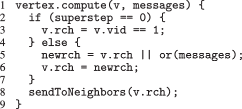
Fig. 1. Incomplete and naive Pregel-like code for all-reachability problem.
Every vertex has a Boolean member variable rch that holds the marking information, that is, whether the vertex is judged to be reachable at the current superstep. The compute function accepts a vertex and its received messages as input. At the first superstep, only the source vertex for which the identifier is one is marked true and the other vertices are marked false. Then each vertex sends its marking information to its neighboring vertices. At the superstep other than the first, each vertex receives incoming messages by “or”ing them, which means that the vertex checks if there is any message containing true. Finally, it “or”s the result and the current rch value, stores the result as the new marking information, and sends it to its neighboring vertices.
Figure 2 demonstrates how three supersteps are used to mark all reachable vertices for an input graph with five vertices. The T and F in the figure stand for true and false, respectively, and the double circle indicates the starting vertex.
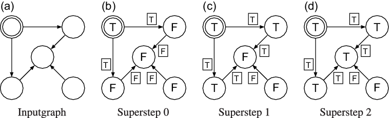
Fig. 2. First three supersteps of the naive program for all-reachability problem.
Though the definition of the compute function is quite simple and easy to understand, the compute function has three apparent inefficiency problems in addition to the non-termination problem.
-
1. A vertex need not send false to its neighboring vertices, because false never switches a neighbor’s rch value to true.
-
2. A vertex need not send true more than once, because sending it only once suffices for marking its neighbors as true.
-
3. It is not necessary to process all vertices at every superstep except the first one. Only those that receive messages from neighbors need to be processed.
The compute function also has two potential inefficiency problems.
-
4. Global barrier synchronization after every superstep might increase overhead. Though Pregel uses synchronous execution, iteration of the compute function could be performed asynchronously without global barrier synchronization.
-
5. Though the compute function is executed independently by every vertex, a set of vertices placed on the same computational node could cooperate for better performance in the computation of vertex values in the set.
The last two inefficiencies have already been recognized, and mechanisms have been proposed to remove them (Gonzalez et al. Reference Gonzalez, Low, Gu, Bickson and Guestrin2012; Yan et al. Reference Yan, Cheng, Lu and Ng2014a).
2.2 Inactivating vertices
To address the apparent inefficiencies, Pregel and many Pregel-like frameworks such as Giraph and Pregel+ introduced an “active” property for each vertex. During iterative execution of the compute function, each vertex is either active or inactive. Initially, all vertices are active. If nothing needs to be done on a vertex, the vertex can become inactive explicitly by voting to halt, which means inactivating itself. At each superstep, only active vertices take part in the calculation of the compute function. An inactive vertex becomes active again by being sent a message from another vertex. The entire iterative processing for a graph terminates when all vertices become inactive and there remain no unreceived messages. Thus, inactivating vertices are used to control program termination.
Figure 3 presents Pregel code for the all-reachability problem that remedies the apparent inefficiencies and also terminates when the rch values on all vertices no longer change.

Fig. 3. Improved Pregel-like code for all-reachability problem.
At the first superstep, only the source vertex is marked true, and it sends its rch value to its neighbors. Then all vertices inactivate themselves by voting to halt. At the second and subsequent supersteps, only those vertices that have messages reactivate, receive the messages, and calculate their newrch values. If newrch and the current rch are not the same, the vertex updates its rch value and sends it to its neighboring vertices. Then, all vertices inactivate again by voting to halt. If newrch and the current rch are the same on all vertices, they inactivate simultaneously, and the iterative computation of the compute function terminates.
As can be seen from the code in Figure 3, to remove the apparent inefficiencies, a compute function based on the Pregel model describes communications and termination control explicitly. This makes defining compute functions unintuitive and difficult.
When aggregations are necessary, the situation becomes worse. For example, suppose that we want to mark the reachable vertices and stop when we have a sufficient number (N) of them. For simplicity, we assume that there are more than 100 reachable vertices in the target graph. We call this problem in which
 $N = 100$
the 100-reachability problem. At each superstep, the compute function needs to count the number of currently reachable vertices to determine whether it should continue or halt. To enable acquiring such global information, Pregel supports a mechanism called aggregation, which collects data from all active vertices and aggregates them by using a specified operation such as sum or max. Each vertex can use the aggregation result in the next superstep. By using aggregation to count the number of vertices that are marked true, we can solve the 100-reachability problem, as shown in the vertex program in Figure 4.
$N = 100$
the 100-reachability problem. At each superstep, the compute function needs to count the number of currently reachable vertices to determine whether it should continue or halt. To enable acquiring such global information, Pregel supports a mechanism called aggregation, which collects data from all active vertices and aggregates them by using a specified operation such as sum or max. Each vertex can use the aggregation result in the next superstep. By using aggregation to count the number of vertices that are marked true, we can solve the 100-reachability problem, as shown in the vertex program in Figure 4.
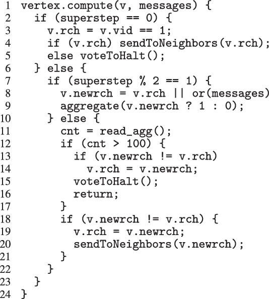
Fig. 4. Pregel-like code for 100-reachability problem.
Note that aggregation should be done before the check for the number of reachable vertices. This order is guaranteed by using the odd supersteps to compute aggregation and the even supersteps to check the number. The programmer must explicitly assign states to supersteps so that different supersteps behave differently. The value of newrch is set in an odd superstep and read in the next even superstep. Since the extent of a local variable is one execution of the compute function in a superstep, newrch has to be changed from a local variable in Figure 3 to a member variable of a vertex in Figure 4.
Only active vertices participate in the aggregation, because inactive vertices do not execute the compute function. Thus, vertices marked true should not inactivate, that is, should not vote to halt, in order to determine the precise number of reachable vertices. This subtle control of inactivation is error-prone no matter how careful the programmer.
The program for the 100-reachability problem shows that explicit state controls and subtle termination controls make the program difficult to describe and understand.
2.3 Asynchronous execution
For the fourth potential inefficiency, asynchronous execution in which vertex computations are processed without global barrier synchronization can be considered instead of synchronous execution. Removing barriers could improve the efficiency of the vertex-centric computation. For the all-reachability problem, both synchronous and asynchronous executions lead to the same solution. Generally speaking, however, both executions do not always yield the same result; this depends on the algorithm. In addition, even if they yield the same result, which execution style of the two is more efficient depends on the situation.
Some vertex-centric frameworks, for example, GiraphAsync (Liu et al. Reference Liu, Zhou, Gao and Fan2016), use asynchronous execution. There are also frameworks that support both synchronous and asynchronous executions, such as GraphLab (Low et al. Reference Low, Gonzalez, Kyrola, Bickson, Guestrin and Hellerstein2012), GRACE (Wang et al. Reference Wang, Xie, Demers and Gehrke2013), and PowerSwitch (Xie et al. Reference Xie, Chen, Guan, Zang and Chen2015).
2.4 Grouping related vertices
For coping with the fifth potential inefficiency, placing a group of related vertices on the same computational node and executing all vertex computation as a single unit of processing could improve efficiency. This means enlarging the processing unit from a single vertex to a set of vertices. Many frameworks have been developed on the basis of this idea. For example, NScale (Quamar et al. Reference Quamar, Deshpande and Lin2014), Giraph++ (Tian et al. Reference Tian, Balmin, Corsten, Tatikonda and McPherson2013), and GoFFish (Simmhan et al. Reference Simmhan, Kumbhare, Wickramaarachchi, Nagarkar, Ravi, Raghavendra and Prasanna2014) are based on subgraph-centric computation, and Blogel (Yan et al. Reference Yan, Cheng, Lu and Ng2014a) is based on block-centric computation. Again, which computation style of the two, vertex-centric or group-based, is more efficient depends on the program.
2.5 Fregel’s approach
Fregel enables the programmer to write vertex-centric programs without the complex controls described in Section 2.2 from the declarative perspective and automatically eliminates the apparent inefficiencies of naturally described programs. Since explicit, complex, and imperative controls over communications, terminations, and so forth are removed from a program, the vertex computation proceeds to a functional description with “peeking” on neighboring vertices to obtain information necessary for computation.
To solve the all-reachability problem in Fregel, the programmer writes a natural functional program that corresponds to the Pregel program presented in Figure 1 with a separately specified termination condition. Depending on the compilation options specified by the programmer, the Fregel compiler applies optimizations for reducing inefficiencies in the program and generates a program that can run in a procedural vertex-centric graph processing framework.
As a solution for the fourth potential inefficiency, we propose a method for removing the barrier synchronization and thereby enabling asynchronous execution. This optimization also enables removing the fifth potential inefficiency. In asynchronous execution, the order of processing vertices does not matter; therefore, a group of related vertices can be processed independently from other groups of vertices. To improve the efficiency of processing vertices in a group, we propose introducing priorities for processing vertices.
3 Functional model for synchronous vertex-centric computation
We first modeled the synchronous vertex-centric computation as a higher-order function. Then, on the basis of this model, we designed Fregel, a functional DSL. In this section, we introduce our functional model by using Haskell notation. The Fregel language will be described in Section 4.
In the original Pregel, data communication is viewed as explicit pushing in which a vertex sends data to another vertex, typically to its adjacent vertex along an outgoing edge. Thus, a Pregel program describes data exchange between two vertices explicitly, for example, by using sendToNeighbors in Figure 1, which results in a program with an imperative form. Since our aim is to create a functional model of vertex-centric computation, the explicit-pushing style, which has a high affinity with imperative programs, is inappropriate.
We thus designed our functional model so that data communication is viewed as implicit pulling in which a vertex pulls (or “peeks at”) data in an adjacent vertex connected by an incoming edge. The iterative computation at each vertex is defined in terms of a function, and its return value, that is, the result of a single repetition, is implicitly sent to the adjacent vertices. Every adjacent vertex also implicitly receives the communicated value via an argument of the function.
3.1 Definition of datatypes
First, we define the datatypes needed for our functional model. Let
 $\mathit{Graph}~a~b$
be the directed graph type, where a is the vertex value type and b is the edge weight type. The vertices have type
$\mathit{Graph}~a~b$
be the directed graph type, where a is the vertex value type and b is the edge weight type. The vertices have type
 $\mathit{Vertex}~a~b$
, and the edges have type
$\mathit{Vertex}~a~b$
, and the edges have type
 ${\mathit{Edge}~a~b}$
. A vertex of type
${\mathit{Edge}~a~b}$
. A vertex of type
 ${\mathit{Vertex}~a~b}$
has a unique vertex identifier (a positive integer value), a value of type a, and a list of incoming edges of type
${\mathit{Vertex}~a~b}$
has a unique vertex identifier (a positive integer value), a value of type a, and a list of incoming edges of type
 ${[\,\mathit{Edge}~a~b\,]}$
. An edge of type
${[\,\mathit{Edge}~a~b\,]}$
. An edge of type
 ${\mathit{Edge}~a~b}$
is a pair of the edge weight of type b and the source vertex of this edge.
${\mathit{Edge}~a~b}$
is a pair of the edge weight of type b and the source vertex of this edge.
 ${\mathit{Graph}~a~b}$
is a list of all vertices, each of which has the type
${\mathit{Graph}~a~b}$
is a list of all vertices, each of which has the type
 ${\mathit{Vertex}~a~b}$
.
${\mathit{Vertex}~a~b}$
.
The definitions of these datatypes are as follows, where
 ${\mathit{{vid}}}$
,
${\mathit{{vid}}}$
,
 ${\mathit{{val}}}$
, and
${\mathit{{val}}}$
, and
 ${\mathit{{is}}}$
are the identifier, value, and incoming edges of the vertex, respectively,
${\mathit{{is}}}$
are the identifier, value, and incoming edges of the vertex, respectively,
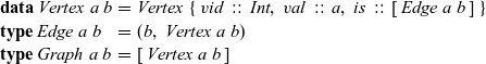 \begin{equation*}\begin{array}{lcl}\textbf{data}~\mathit{Vertex}~a~b & = & \mathit{Vertex}~\{~\mathit{vid}~::~\mathit{Int},~\mathit{val}~::~a,~\mathit{is}~::~[\,\mathit{Edge}~a~b\,]~\} \\\textbf{type}~\mathit{Edge}~a~b & = & (b,~\mathit{Vertex}~a~b) \\\textbf{type}~\mathit{Graph}~a~b & = & [\,\mathit{Vertex}~a~b\,]\end{array}\end{equation*}
For simplicity, we assume that continuous identifiers starting from one are assigned to vertices and that all vertices in a list representing a graph are ordered by their vertex identifiers. As an example, the graph in Figure 2(d) can be defined by the following data structure, where
 ${\mathit{v1}}$
,
${\mathit{v1}}$
,
 ${\mathit{v2}}$
,
${\mathit{v2}}$
,
 ${\mathit{v3}}$
,
${\mathit{v3}}$
,
 ${\mathit{v4}}$
, and
${\mathit{v4}}$
, and
 ${\mathit{v5}}$
are the upper-left, upper-right, lower-left, middle, and lower-right vertices, respectively. We assume that all edges have weight 1:
${\mathit{v5}}$
are the upper-left, upper-right, lower-left, middle, and lower-right vertices, respectively. We assume that all edges have weight 1:
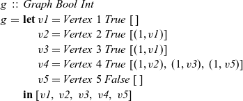 \begin{equation*}\begin{array}{lcl}g & :: & \mathit{Graph}~\mathit{Bool}~\mathit{Int} \\g & = & \textbf{let}~\mathit{v1} = Vertex~1~True~[\,] \\ & & \phantom{\textbf{let}}~\mathit{v2} = Vertex~2~True~[(1, \mathit{v1})] \\ & & \phantom{\textbf{let}}~\mathit{v3} = Vertex~3~True~[(1, \mathit{v1})] \\ & & \phantom{\textbf{let}}~\mathit{v4} = Vertex~4~True~[(1,\mathit{v2}),~(1,\mathit{v3}),~(1,\mathit{v5})] \\ & & \phantom{\textbf{let}}~\mathit{v5} = Vertex~5~False~[\,] \\ & & \textbf{in}~[\mathit{v1},~\mathit{v2},~\mathit{v3},~\mathit{v4},~\mathit{v5}]\end{array}\end{equation*}
3.2 Description of our model
In synchronous vertex-centric parallel computation, each vertex periodically and synchronously performs the following processing steps, which collectively we call a logical superstep, or LSS for short.
-
1. Each vertex receives the data computed in the previous LSS from the adjacent vertices connected by incoming edges.
-
2. In accordance with the problem to be solved, the vertex performs its respective computation using the received data, the data it computed in the previous LSS, and the weights of the incoming edges. If necessary, the vertex acquires global information using aggregation during computation.
-
3. The vertex sends the result of the computation to all adjacent vertices along its outgoing edges. The adjacent vertices receive the data in the next LSS.
These three processing steps are performed in each LSS. An LSS represents a semantically connected sequence of actions at each vertex. Each vertex repeatedly executes this “sequence of actions.” An LSS is “logical” in the sense that it might contain aggregation and thus might take more than one Pregel superstep. We represent an LSS as a single function and call it an LSS function. As explained earlier, an LSS function does not explicitly describe sending and receiving data between a vertex and the adjacent vertices.
The arguments given to an LSS function are an integer value called the clock and the vertex on which the LSS function is repeatedly performed. A clock represents the number of iterations of the LSS function. Note that the result of an LSS function may have a type different from that of the vertex value. Thus, the type of an LSS function is
 ${\mathit{Int}\rightarrow \mathit{Vertex}~a~b \rightarrow r}$
, where a is the vertex value type and r is the result type.
${\mathit{Int}\rightarrow \mathit{Vertex}~a~b \rightarrow r}$
, where a is the vertex value type and r is the result type.
We express the LSS function using two functions. One is an initialization function, which defines the behavior when the clock is 0, and the other is a step function, which defines the behavior when the clock is greater than 0. Let t be a clock value. The initialization function takes as its argument a vertex and returns the result for
 ${t = 0}$
. Thus, its type is
${t = 0}$
. Thus, its type is
 ${\mathit{Vertex}~a~b \rightarrow r}$
. The step function takes three arguments: the result for the vertex at the previous clock, a list of pairs, each of which is composed by the weight of an incoming edge and the result of the adjacent vertex connected by the edge at the previous clock, and the vertex itself. Thus, its type is
${\mathit{Vertex}~a~b \rightarrow r}$
. The step function takes three arguments: the result for the vertex at the previous clock, a list of pairs, each of which is composed by the weight of an incoming edge and the result of the adjacent vertex connected by the edge at the previous clock, and the vertex itself. Thus, its type is
 ${r \rightarrow [(b,r)] \rightarrow \mathit{Vertex}~a~b \rightarrow r}$
. On the basis of these two functions, a general form of the LSS function is defined in terms of
${r \rightarrow [(b,r)] \rightarrow \mathit{Vertex}~a~b \rightarrow r}$
. On the basis of these two functions, a general form of the LSS function is defined in terms of
 ${\mathit{lssGeneral}}$
, which can be defined as a fold-like second-order function as follows:
${\mathit{lssGeneral}}$
, which can be defined as a fold-like second-order function as follows:
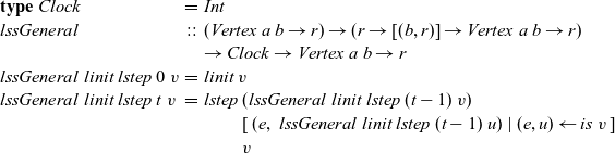 \begin{equation*}\begin{array}{lcl}\textbf{type}~Clock &=& \mathit{Int} \\\mathit{lssGeneral} &::& (\mathit{Vertex}~a~b \rightarrow r) \rightarrow (r \rightarrow [(b,r)] \rightarrow \mathit{Vertex}~a~b \rightarrow r) \\ & & \rightarrow Clock \rightarrow \mathit{Vertex}~a~b \rightarrow r \\lssGeneral~linit~lstep~0~v &=& linit~v \\lssGeneral~linit~lstep~t~v &=& lstep~(\mathit{lssGeneral}~linit~lstep~(t-1)~v) \\ & & \phantom{lstep}~ [\>{(e,~\mathit{lssGeneral}~linit~lstep~(t-1)~u)}~|~{(e,u)} \leftarrow {\mathit{is}~v}{}\,] \\ & & \phantom{lstep}~v\end{array}\end{equation*}
An LSS function, lss, for a specific problem is defined by giving appropriate initialization and step functions,
 ${\mathit{ainit}}$
and
${\mathit{ainit}}$
and
 ${\mathit{astep}}$
, as actual arguments to
${\mathit{astep}}$
, as actual arguments to
 ${\mathit{lssGeneral}}$
, that is,
${\mathit{lssGeneral}}$
, that is,
 ${\mathit{lss}~=~\mathit{lssGeneral}~\mathit{ainit}~\mathit{astep}}$
.
${\mathit{lss}~=~\mathit{lssGeneral}~\mathit{ainit}~\mathit{astep}}$
.
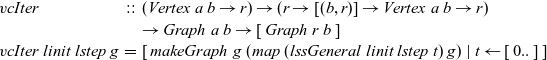
Let
 ${g = [\,v_1,~v_2,~v_3,~\ldots\,]}$
be the target graph of type
${g = [\,v_1,~v_2,~v_3,~\ldots\,]}$
be the target graph of type
 ${\mathit{Graph}~a~b}$
of the computation, where we assume that the identifier of
${\mathit{Graph}~a~b}$
of the computation, where we assume that the identifier of
 ${v_k}$
is k. The list of computation results of LSS function
${v_k}$
is k. The list of computation results of LSS function
 ${\mathit{lss}}$
on all vertices in the graph at clock t is
${\mathit{lss}}$
on all vertices in the graph at clock t is
 ${[\,\mathit{lss}~t~v_1,~\mathit{lss}~t~v_2,~\mathit{lss}~t~v_2,~\ldots\,] :: [\,r\,]}$
. Further, let
${[\,\mathit{lss}~t~v_1,~\mathit{lss}~t~v_2,~\mathit{lss}~t~v_2,~\ldots\,] :: [\,r\,]}$
. Further, let
 ${g_t}$
be a graph constructed from the results of
${g_t}$
be a graph constructed from the results of
 ${\mathit{lss}}$
on all vertices at clock t, that is,
${\mathit{lss}}$
on all vertices at clock t, that is,
 ${g_t = \mathit{makeGraph}~g~[\,\mathit{lss}~t~v_1,~\mathit{lss}~t~v_2,~\mathit{lss}~t~v_3,~\ldots\,]}$
. Here,
${g_t = \mathit{makeGraph}~g~[\,\mathit{lss}~t~v_1,~\mathit{lss}~t~v_2,~\mathit{lss}~t~v_3,~\ldots\,]}$
. Here,
 ${\mathit{makeGraph}~g~[\,r_1,~r_2,~\ldots\,]}$
returns a graph with the same shape as g for which the i-th vertex has the value
${\mathit{makeGraph}~g~[\,r_1,~r_2,~\ldots\,]}$
returns a graph with the same shape as g for which the i-th vertex has the value
 ${r_i}$
and the edges have the same weights as those in g:
${r_i}$
and the edges have the same weights as those in g:
 \begin{equation*}\begin{array}{lcl}\mathit{makeGraph} &::& \mathit{Graph}~a~b \rightarrow [\,r\,] \rightarrow \mathit{Graph}~r~b\\\mathit{makeGraph}~g~xs &=& newg\\ & & \textbf{where}~newg~=\\ & & \phantom{\textbf{where}~}\>[\>\mathit{Vertex}~k~(xs~!!~(k-1))\\ & & \phantom{\textbf{where}~\>[\>\mathit{Vertex}~} [\>{(e,~newg~!!~(k'-1))}~|~{(e,~\mathit{Vertex}~k'~\_~\_)} \leftarrow {es}{}\,]\\ & & \phantom{\textbf{where}~\>[\>}~|~\mathit{Vertex}~k~\_~es \leftarrow g\>]\end{array}\end{equation*}
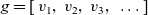
Then the infinite stream (list) of graphs
 ${[\,g_0,~g_1,~g_2,~\ldots\,]}$
represents infinite iterations of LSS function
${[\,g_0,~g_1,~g_2,~\ldots\,]}$
represents infinite iterations of LSS function
 ${\mathit{lss}}$
. This infinite stream can be produced by using the higher-order function
${\mathit{lss}}$
. This infinite stream can be produced by using the higher-order function
 ${\mathit{vcIter}}$
, which takes as its arguments initialization and step functions and a target graph represented by a list of vertices:
${\mathit{vcIter}}$
, which takes as its arguments initialization and step functions and a target graph represented by a list of vertices:
 \begin{equation*}\begin{array}{lcl}\mathit{vcIter} &::& (\mathit{Vertex}~a~b \rightarrow r) \rightarrow (r \rightarrow [(b,r)] \rightarrow \mathit{Vertex}~a~b \rightarrow r) \\ & & \rightarrow \mathit{Graph}~a~b \rightarrow [\,\mathit{Graph}~r~b\,] \\\mathit{vcIter}~linit~lstep~g &=& [\>{\mathit{makeGraph}~g~(map~(\mathit{lssGeneral}~linit~lstep~t)~g)}~|~{t} \leftarrow {[\,0..\,]}{}\,]\end{array}\end{equation*}
Though
 ${\mathit{vcIter}}$
produces an infinite stream of graphs, we want to terminate its computation at an appropriate clock and return the graph at this clock as the final result. We can give a termination condition to the infinite sequence from outside and obtain the desired result by using
${\mathit{vcIter}}$
produces an infinite stream of graphs, we want to terminate its computation at an appropriate clock and return the graph at this clock as the final result. We can give a termination condition to the infinite sequence from outside and obtain the desired result by using
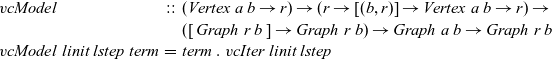
 ${\mathit{term}~(\mathit{vcIter}~linit~lstep~g)}$
, where
${\mathit{term}~(\mathit{vcIter}~linit~lstep~g)}$
, where
 ${\mathit{term}}$
selects the desired final result from the sequence of graphs to terminate the computation.
${\mathit{term}}$
selects the desired final result from the sequence of graphs to terminate the computation.
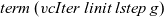
Figure 5 presents example termination functions. A typical termination point is when the computation falls into a steady state, after which graphs in the infinite list never change. The termination function fixedValue returns the graph of the steady state of a given infinite list. Another termination point is when a graph in the stream comes to satisfy a specified condition. We can use the higher-order termination function untilValue for this case. It takes a predicate function specifying the desired condition and returns the first graph that satisfies this predicate from a given infinite stream. Finally, nthValue retrieves the graph at a given clock.
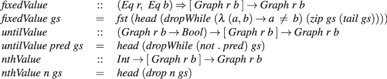
Fig. 5. Termination functions.
We define
 ${\mathit{vcModel}}$
as the composition of a termination function and
${\mathit{vcModel}}$
as the composition of a termination function and
 ${\mathit{vcIter}}$
. We regard the function
${\mathit{vcIter}}$
. We regard the function
 ${\mathit{vcModel}}$
as representing functional vertex-centric graph processing:
${\mathit{vcModel}}$
as representing functional vertex-centric graph processing:
 \begin{equation*}\begin{array}{lcl}\mathit{vcModel} &::& (\mathit{Vertex}~a~b \rightarrow r) \rightarrow (r \rightarrow [(b,r)] \rightarrow \mathit{Vertex}~a~b \rightarrow r) \rightarrow \\ & & ([\,\mathit{Graph}~r~b\,] \rightarrow \mathit{Graph}~r~b) \rightarrow \mathit{Graph}~a~b \rightarrow \mathit{Graph}~r~b \\\mathit{vcModel}~linit~lstep~\mathit{term} &=& \mathit{term}~.~\mathit{vcIter}~linit~lstep\end{array}\end{equation*}
An LSS function defined in terms of
 ${\mathit{lssGeneral}}$
has a recursive form on the basis of the structure of the input graph. Although a graph has a recursive structure, a recursive call of an LSS function does not cause an infinite recursion, because a recursive call always uses the prior clock, that is,
${\mathit{lssGeneral}}$
has a recursive form on the basis of the structure of the input graph. Although a graph has a recursive structure, a recursive call of an LSS function does not cause an infinite recursion, because a recursive call always uses the prior clock, that is,
 ${t-1}$
.
${t-1}$
.
3.3 Simple example
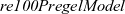
Figure 6 presents the formulation of the reachability problems on the basis of the proposed functional model, where reAllPregelModel is for the all-reachablity problem and
 ${\mathit{re100PregelModel}}$
is for the 100-reachability problem. Variable numTrueVertices is the number of vertices with a value of True for the target graph. The only difference between these two formulations is the termination condition; the all-reachability problem formulation uses fixedValue, while the 100-reachability problem one uses untilValue. Note that the LSS function characterized by reInit and reStep has no description for the aggregation that appears in the original Pregel code (Figure 4).
${\mathit{re100PregelModel}}$
is for the 100-reachability problem. Variable numTrueVertices is the number of vertices with a value of True for the target graph. The only difference between these two formulations is the termination condition; the all-reachability problem formulation uses fixedValue, while the 100-reachability problem one uses untilValue. Note that the LSS function characterized by reInit and reStep has no description for the aggregation that appears in the original Pregel code (Figure 4).
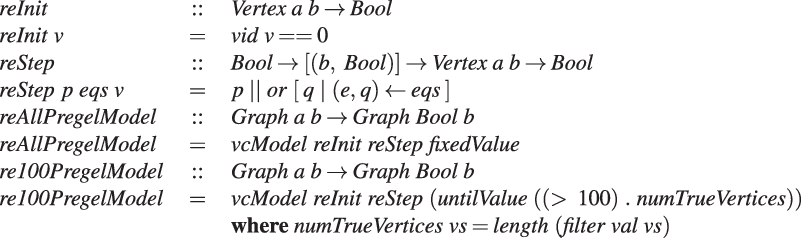
Fig. 6. Formulation of reachability problems in our model.
3.4 Limitations of our model
Our model suffers the following limitations:
-
Data can be exchanged only between adjacent vertices.
-
A vertex cannot change the shape of the graph or the weight of an edge.
In the Pregel model, a vertex can send data to a vertex other than the adjacent ones as long as it can specify the destination vertex. In our model, unless global aggregation is used, data can be exchanged only between adjacent vertices directly connected by a directed edge. A vertex-centric graph processing model with this limitation, which is sometimes called the GAS (gather-apply-scatter) model, has been used by many researchers (Gonzalez et al. Reference Gonzalez, Low, Gu, Bickson and Guestrin2012; Bae & Howe Reference Bae and Howe2015; Sengupta et al., Reference Sengupta, Song, Agarwal and Schwan2015).
Furthermore, in our model, computation on a vertex cannot change the shape of the graph or weight of an edge. This limitation makes it is impossible to represent some algorithms including those based on the pointer jumping technique. However, even under this additional limitation, many practical graph algorithms can be described.The Fregel language inherits these limitations because it was designed on the basis of our model. As mentioned in Section 1, removing these limitations from the Fregel language is left for future work.
3.5 Features of our model
Our model has four notable features.
First, our model is purely functional; computation that is periodically and synchronously performed at every vertex is defined as an LSS function without any side effects that have the form of a structural recursion on the graph structure. The recursive execution of such an LSS function is regarded as dynamic programming on the graph on the basis of memorization.
Second, an LSS function does not have explicit descriptions for sending or receiving data between adjacent vertices. Instead, it uses recursive calls of the LSS function for adjacent vertices, which can be regarded as an implicit pulling style of communication.
Third, an LSS function enables the programmer to describe a series of processing steps as a whole that could be unwillingly divided into small supersteps due to barrier synchronization in the BSP model if we used the original Pregel model.
Fourth, the entire computation for a graph is represented as an infinite list of resultant graphs in ascending clock time order. The LSS function has no description for the termination of the computation. Instead, termination is described by a function that appropriately chooses the desired result from an infinite list.
4 Fregel functional domain-specific language
Fregel is a functional DSL for declarative-style programming on large-scale graphs that uses computation based on
 ${\mathit{vcModel}}$
(defined in Section 3). A Fregel program can be run on Haskell interpreters like GHCi, because Fregel’s syntax follows that of Haskell. This ability is useful for testing and debugging a Fregel program. After testing and debugging, the Fregel program can be compiled into a program for a Pregel-like framework such as Giraph and Pregel+.
${\mathit{vcModel}}$
(defined in Section 3). A Fregel program can be run on Haskell interpreters like GHCi, because Fregel’s syntax follows that of Haskell. This ability is useful for testing and debugging a Fregel program. After testing and debugging, the Fregel program can be compiled into a program for a Pregel-like framework such as Giraph and Pregel+.
4.1 Main features of Fregel
Fregel captures data access, data aggregation, and data communication in a functional manner and supports concise ways of writing various graph computations in a compositional manner through the use of four second-order functions. Fregel has three main features.
First, Fregel abstracts access to vertex data by using three tables indexed by vertices. The prev table is used to access vertex data (i.e., results of recursive calls of the step function) at the previous clock. The curr table is used to access vertex data at the current clock. These two tables explicitly implement the memorization of calculated values. The third table, val is used to access vertex initial values, that is, the values placed on vertices when the computation started. An index given to a table is neither the identifier of a vertex nor the position of a vertex in a list of incoming edges but rather is a vertex itself. This enables the programmer to write in a more “direct” style for data accesses.
Second, Fregel abstracts aggregation and communication by using a comprehension with a specific generator. Aggregation is described by a comprehension for which the generator is the entire graph (list of all vertices), while communication with adjacent vertices is described by a comprehension for which the generator is the list of adjacent vertices.
Third, Fregel is equipped with four second-order functions for graphs, which we call second-order graph functions. A Fregel program can use these functions multiple times. Function
fregel
corresponds to functional model
 ${\mathit{vcModel}}$
defined in Section 3. Function
gzip
pairs values for the corresponding vertices in two graphs of the same shape, and
gmap
applies a given function to every vertex. Function
giter
abstracts iterative computation.
${\mathit{vcModel}}$
defined in Section 3. Function
gzip
pairs values for the corresponding vertices in two graphs of the same shape, and
gmap
applies a given function to every vertex. Function
giter
abstracts iterative computation.
In the following sections, we first introduce the core part of the Fregel language constructs and then explain Fregel programming by using some specific examples.
4.2 Fregel language constructs
A vertex in the functional model described in Section 3.1 has a list of adjacent vertices connected by incoming edges. However, some graph algorithms use edges for the reverse direction. For example, the min-label algorithm (Yan et al. Reference Yan, Cheng, Xing, Lu, Ng and Bu2014b) for calculating strongly connected components of a given graph, which is described in Section 4.6, needs backward propagation in which a vertex sends messages toward its neighbors connected by its incoming edges. In our implicit pulling style of communications, this means that a vertex needs to peek at data in an adjacent vertex connected by an outgoing edge. Thus, though different from the functional model, we decided to let every vertex have two lists of edges: one contains incoming edges in the original graph and the other contains incoming edges in the reversed (transposed) graph. An incoming edge in the reversed graph is an edge produced by reversing an outgoing edge in the original graph. This makes it easier for the programmer to write programs in which part of the computation needs to be carried out on the reversed graph. Hereafter, a “reversed edge” means an edge in the latter list.
Figure 7 presents the syntax of Fregel. Other than the normal reserved words in bold font, the tokens in bold-slant font are important reserved words like identifier names and data constructor names in Fregel. Program examples of Fregel can be found from Sections 4.3 to 4.6. Please refer to these examples as needed.

Fig. 7. Core part of Fregel syntax.
A Fregel program defines the main function,
 $\langle{{mainFn}}\rangle$
, which takes a single input graph and returns a resultant graph. In the program body, the resultant graph is specified by a graph expression,
$\langle{{mainFn}}\rangle$
, which takes a single input graph and returns a resultant graph. In the program body, the resultant graph is specified by a graph expression,
 $\langle{{graphExpr}}\rangle$
, which can construct a graph using the four second-order graph functions.
$\langle{{graphExpr}}\rangle$
, which can construct a graph using the four second-order graph functions.
Second-order graph function
fregel
, which is probably the most frequently used function by the programmer, corresponds to
 ${\mathit{vcModel}}$
and defines the iterative behavior of an LSS. As described above, it is abstracted as two functions: the initialization function (the first argument) and the step function (the second argument), which is repeatedly executed.
${\mathit{vcModel}}$
and defines the iterative behavior of an LSS. As described above, it is abstracted as two functions: the initialization function (the first argument) and the step function (the second argument), which is repeatedly executed.
The initialization function of
fregel
is the same as that of
 ${\mathit{vcModel}}$
. It takes a vertex of type
${\mathit{vcModel}}$
. It takes a vertex of type
 ${\mathit{Vertex}~a~b}$
as its only argument and returns an initial value of type r for the iteration carried out by the step function. On the other hand, a step function of
fregel
is slightly different.
${\mathit{Vertex}~a~b}$
as its only argument and returns an initial value of type r for the iteration carried out by the step function. On the other hand, a step function of
fregel
is slightly different.
-
First, the step function of
 ${\mathit{vcModel}}$
executed on every vertex is passed its own result and those of adjacent vertices at the previous clock, together with the weights of incoming edges, through its arguments. In contrast, the step function of
fregel
takes a
prev
table from which the results of every vertex at the previous clock can be obtained. Edge weights are not explicitly passed to the step function. They can be obtained by using a comprehension for which the generator is the list of adjacent vertices.
${\mathit{vcModel}}$
executed on every vertex is passed its own result and those of adjacent vertices at the previous clock, together with the weights of incoming edges, through its arguments. In contrast, the step function of
fregel
takes a
prev
table from which the results of every vertex at the previous clock can be obtained. Edge weights are not explicitly passed to the step function. They can be obtained by using a comprehension for which the generator is the list of adjacent vertices. -
Second, fregel ’s step function takes another table called curr , which holds the results at the current clock for the cases in which these values are necessary for computing the results for the current LSS. We show an example of using the curr table in Section 4.5.
-
Third, while the termination judgment of
${\mathit{vcModel}}$
is made using a function that chooses a desired graph from a stream of graphs, that of
fregel
is not a function.


Since the initialization and step functions return multiple values in many cases, the programmer must often define a record,
 $\langle{{recordDef}}\rangle$
, for them before the main function and let each vertex hold the record data. Fregel provides a concise way to access a record field by using the field selection operator denoted by
$\langle{{recordDef}}\rangle$
, for them before the main function and let each vertex hold the record data. Fregel provides a concise way to access a record field by using the field selection operator denoted by
 $.\wedge$
, which resembles the ones in Pascal and C.
$.\wedge$
, which resembles the ones in Pascal and C.
Second-order graph function giter iterates a specified computation on a graph. Similar to fregel , it takes two functions: the initialization function iinit as its first argument and the iteration function iiter as its second argument. Let a and b be the vertex value type and edge weight type in the input graph, respectively, and let r be the vertex value type in the output graph. The following iterative computation is performed by giter , where g is the input graph:
 \begin{equation*}\begin{array}{l}g\>\mathbin{::}\>\mathit{Graph}~a~b~~\smash{\mathop{\longrightarrow}\limits^{iinit}}~~g_0\>\mathbin{::}\>\mathit{Graph}~r~b~~\smash{\mathop{\longrightarrow}\limits^{iiter}}~~g_1\>\mathbin{::}\>\mathit{Graph}~r~b\\[1.5mm]\smash{\mathop{\longrightarrow}\limits^{iiter}}~~\cdots~~\smash{\mathop{\longrightarrow}\limits^{iiter}}~~g_n\>\mathbin{::}\>\mathit{Graph}~r~b\end{array}\end{equation*}
First, before entering the iteration, iinit is applied to every vertex in input graph g to produce the initial graph
 ${g_0}$
of the iteration. Then iiter is repeatedly called to produce successive graphs,
${g_0}$
of the iteration. Then iiter is repeatedly called to produce successive graphs,
 ${g_1}, \ldots, {g_n}$
. The iteration terminates when the termination condition given as the third argument of
giter
is satisfied. The Haskell definition of
giter
in the Fregel interpreter, which may help the reader understand the behavior of
giter
, is presented in Section 5. Different from
fregel
’s step function,
giter
’s iteration function, iiter, takes a graph and returns the next graph, possibly by using second-order graph functions. Since
giter
is used for repeating
fregel
,
gmap
, etc., it takes only a graph. Section 4.6 presents an example of using
giter
.
${g_1}, \ldots, {g_n}$
. The iteration terminates when the termination condition given as the third argument of
giter
is satisfied. The Haskell definition of
giter
in the Fregel interpreter, which may help the reader understand the behavior of
giter
, is presented in Section 5. Different from
fregel
’s step function,
giter
’s iteration function, iiter, takes a graph and returns the next graph, possibly by using second-order graph functions. Since
giter
is used for repeating
fregel
,
gmap
, etc., it takes only a graph. Section 4.6 presents an example of using
giter
.
The termination condition,
 $\langle{{termination}}\rangle$
, is specified for the third argument of
fregel
and
giter
. This is not a function like fixedValue in the functional model, but a data represented by a data constructor like
Fix
,
Until
, or
Iter
, where
Fix
means a steady state,
Until
means a termination condition specified by a predicate function, and
Iter
specifies the number of iterations to perform.
$\langle{{termination}}\rangle$
, is specified for the third argument of
fregel
and
giter
. This is not a function like fixedValue in the functional model, but a data represented by a data constructor like
Fix
,
Until
, or
Iter
, where
Fix
means a steady state,
Until
means a termination condition specified by a predicate function, and
Iter
specifies the number of iterations to perform.
The expressions in Fregel are standard expressions in Haskell, field access expressions on a vertex (
 $\langle{fieldAccess}\rangle$
), and aggregation expressions (
$\langle{fieldAccess}\rangle$
), and aggregation expressions (
 $\langle{comAggr}\rangle$
) each of which applies a combining function to a comprehension with specific generators. There are three generators in Fregel; (1) a graph variable to generate all vertices in a graph, (2)
$\langle{comAggr}\rangle$
) each of which applies a combining function to a comprehension with specific generators. There are three generators in Fregel; (1) a graph variable to generate all vertices in a graph, (2)
 ${\boldsymbol{is}~v}$
where v is a vertex variable to generate all pairs of v’s adjacent vertices connected by incoming edges and the edge weights, and (3)
${\boldsymbol{is}~v}$
where v is a vertex variable to generate all pairs of v’s adjacent vertices connected by incoming edges and the edge weights, and (3)
 ${\boldsymbol{rs}~v}$
where v is a vertex variable to generate all pairs of v’s adjacent vertices connected by reversed edges and the edge weights. A combining function is one of the six standard functions that have both commutative and associative properties such as minimum.
${\boldsymbol{rs}~v}$
where v is a vertex variable to generate all pairs of v’s adjacent vertices connected by reversed edges and the edge weights. A combining function is one of the six standard functions that have both commutative and associative properties such as minimum.
Though Fregel is syntactically a subset of Haskell, Fregel has the following restrictions:
-
Recursive definitions are not allowed in a let expression. This means that the programmer cannot define (mutually) recursive functions nor variables with circular dependencies.
-
Lists and functions cannot be used as values except for functions given as arguments to second-order graph functions.
-
A user-defined record has to be non-recursive.
-
A specified data obtained from the curr table have to be already determined.
Due to these restrictions, circular dependent values cannot appear in a Fregel program. Thus, Fregel programs do not rely on laziness. In fact, the Fregel compiler compiles a Fregel program into a Java or C++ program that computes non-circular dependent values one by one without the need for lazy evaluation.
4.3 Examples: reachability problems
Our first example Fregel program is one for solving the all-reachability problem (Figure 8(a)). Since the LSS for this problem calculates a Boolean value indicating whether each vertex is currently reachable or not, we define a record RVal that contains only this Boolean value at the rch field in this record.

Fig. 8. Fregel programs for solving reachability problems.
Function reAll, the main part of the program, defines the initialization and step functions. The initialization function, reInit, returns an RVal record in which the rch field is True only if the vertex is the starting point (vertex identifier is one). The vertex identifier can be obtained by using a special predefined function,
vid
. The step function, reStep, collects data at the previous clock from every adjacent vertex connected by an incoming edge. This is done by using the syntax of comprehension, in which the generator is
 ${\boldsymbol{is}~v}$
. For every adjacent vertex u, this program obtains the result at the previous clock by using
prev u and accesses its rch field. Then, reStep combines the results of all adjacent vertices by using the
${\boldsymbol{is}~v}$
. For every adjacent vertex u, this program obtains the result at the previous clock by using
prev u and accesses its rch field. Then, reStep combines the results of all adjacent vertices by using the
 ${\mathit{or}}$
function and returns the disjunction of the combined value and its respective rch value at the previous clock.
${\mathit{or}}$
function and returns the disjunction of the combined value and its respective rch value at the previous clock.
In reAll, reInit and reStep are given to the fregel function. Its third argument, Fix , specifies the termination condition, and the fourth argument is the input graph.
Figure 8(b) presents a Fregel program for solving the 100-reachability problem. This program is the same as that in Figure 8(a) except for the termination condition. The termination condition in this program uses Until , which corresponds to untilValue in our functional model. Until takes a function that defines the condition. This function gathers the number of currently reachable vertices by aggregation. Fregel’s aggregation takes the form of a comprehension for which the generator is the input graph, that is, a list of all vertices.
Note that both the initialization and step functions are common to both reAll and
 ${\mathit{re100}}$
. The only difference between them is the termination condition: reAll specifies
Fix
and
${\mathit{re100}}$
. The only difference between them is the termination condition: reAll specifies
Fix
and
 ${\mathit{re100}}$
specifies
Until
. The common step function describes only how to calculate the value of interest (whether or not each vertex is reachable). A description related to termination is not included in the definition of the step function. Instead, it is specified as the third argument of
fregel
. This is in sharp contrast to the programs in the original Pregel (Figures 3 and 4), in which each vertex’s transition to the inactive state is explicitly described in the compute function.
${\mathit{re100}}$
specifies
Until
. The common step function describes only how to calculate the value of interest (whether or not each vertex is reachable). A description related to termination is not included in the definition of the step function. Instead, it is specified as the third argument of
fregel
. This is in sharp contrast to the programs in the original Pregel (Figures 3 and 4), in which each vertex’s transition to the inactive state is explicitly described in the compute function.
4.4 Example: calculating diameter
The next example calculates the diameter of a graph whose endpoints include the vertex with identifier one. This example sequentially calls two
fregel
functions, each of which is similar to the reachability computation. The input is assumed to be a connected undirected graph. In Fregel, an undirected edge between two vertices
 ${v_1}$
and
${v_1}$
and
 ${v_2}$
is represented by two directed edges: one from
${v_2}$
is represented by two directed edges: one from
 ${v_1}$
to
${v_1}$
to
 ${v_2}$
and the other from
${v_2}$
and the other from
 ${v_2}$
to
${v_2}$
to
 ${v_1}$
.
${v_1}$
.
The first call uses values on edges to find the shortest path length from the source vertex (vertex identifier one) to every vertex. This is known as the single-source shortest path problem. The second one finds the maximum value of the shortest path lengths of all vertices.
Figure 9 presents the program. The LSS for the first
fregel
calculates the tentative shortest path length to every vertex from the source vertex, so record
 ${\mathit{{SVal}}}$
consists of an integer field
${\mathit{{SVal}}}$
consists of an integer field
 ${\mathit{{dist}}}$
. The step function ssspStep of the first
fregel
uses the edge weights, that is, the first component e of the pair generated in the comprehension, to update the tentative shortest path for a vertex. It takes the minimum sum of the tentative shortest path of every neighbor vertex (
${\mathit{{dist}}}$
. The step function ssspStep of the first
fregel
uses the edge weights, that is, the first component e of the pair generated in the comprehension, to update the tentative shortest path for a vertex. It takes the minimum sum of the tentative shortest path of every neighbor vertex (
 ${\boldsymbol{prev}~{u}~.\wedge~{dist}}$
) and the edge length (e) from the neighbor vertex.
${\boldsymbol{prev}~{u}~.\wedge~{dist}}$
) and the edge length (e) from the neighbor vertex.
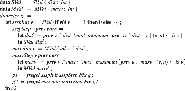
Fig. 9. Fregel program for calculating diameter.
In the second fregel , every vertex holds the tentative maximum value in the record MVal among the values transmitted to the vertex so far. In its step function, maxvStep, every vertex receives the tentative maximum values of the adjacent vertices connected by incoming edges, calculates the maximum of the received values and its previous tentative value, and updates the tentative value.
The output graph of the first
fregel
,
 ${\mathit{g1}}$
, is input to the second
fregel
, and its resultant graph is the final answer, in which every vertex has the value of the diameter.
${\mathit{g1}}$
, is input to the second
fregel
, and its resultant graph is the final answer, in which every vertex has the value of the diameter.
4.5 Example: reachability with ranking
Next, we present an example of using the curr table. The reachability with ranking problem is essentially the same as the all-reachability problem except that it also determines the ranking of every reachable vertex, where ranking r means that the number of steps to the reachable vertex is ranked in the top r among all vertices. A Fregel program for solving this problem is presented in Figure 10.
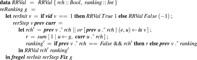
Fig. 10. Fregel program for solving reachability with ranking problem.
We define a record RRVal with two fields: rch (which is the same as that in RVal in the other reachability problems) and ranking. For the source vertex, the initialization function, rerInit, returns an RRVal record in which the rch and ranking fields are True and 1, respectively. For every other vertex, it returns an RRVal record in which rch is False and ranking is
 $-1$
, which means that the ranking is undetermined. The step function, rerStep, calculates the new rch field value in the same manner as for the other reachability problems. In addition, it calculates the number of reachable vertices at the current LSS by using the global aggregation, for which the generator is the entire graph with the
$-1$
, which means that the ranking is undetermined. The step function, rerStep, calculates the new rch field value in the same manner as for the other reachability problems. In addition, it calculates the number of reachable vertices at the current LSS by using the global aggregation, for which the generator is the entire graph with the
 ${\mathit{sum}}$
operator. To do this, it filters out the vertices that have not been reached yet. Writing this aggregation as:
${\mathit{sum}}$
operator. To do this, it filters out the vertices that have not been reached yet. Writing this aggregation as:
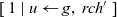 \begin{equation*}\begin{array}{l}[\>{1}~|~{u} \leftarrow {g}{,~rch'}\,]\end{array}\end{equation*}
is incorrect because rch’ is not a local variable on a remote vertex u but rather a local variable on the vertex v that is executing rerStep. To enable v to refer to the rch’ value of the current LSS on a remote vertex u, it is necessary for u to store the value in an RRVal structure by returning an RRVal containing the current rch’ as the result of rerStep. Vertex v can then access the value by
 ${\boldsymbol{curr}~{u}~.\wedge~{rch}}$
.
${\boldsymbol{curr}~{u}~.\wedge~{rch}}$
.
4.6 Example: strongly connected components
As an example of a more complex combination of second-order graph functions, Figure 11 presents a Fregel program for solving the strongly connected components problem. The output of this program is a directed graph with the same shape as the input graph; the value on each vertex is the identifier of the component, that is, the minimum of the vertex identifiers in the component to which it belongs.
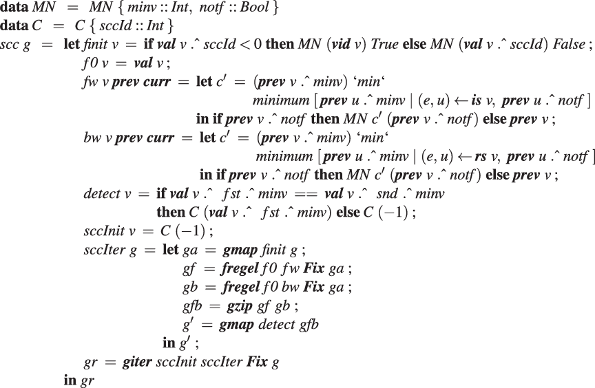
Fig. 11. Fregel program for solving strongly connected components problem.
This program is based on the min-label algorithm (Yan et al. Reference Yan, Cheng, Xing, Lu, Ng and Bu2014b). It repeats four operations until every vertex belongs to a component.
-
(1). Initialization: Every vertex for which a component has not yet been found sets the notf flag value. This means that the vertex must participate in the following computation.
-
(2). Forward propagation: Each notf vertex first sets its minv value as its identifier. Then it repeatedly calculates the minimum value of its (previous) minv value and the minv values of the adjacent vertices connected by incoming edges. This is repeated until the computation falls into a steady state.
-
(3). Backward propagation: This is the same as forward propagation except that the direction of minv propagation is reversed; each
${\mathit{{notf}}}$
vertex updates its minv value through the reversed edges. -
(4). Component detection: Each
${\mathit{{notf}}}$
vertex judges whether the results (identifiers) of forward propagation and backward propagation are the same. If they are, the vertex belongs to the component represented by the identifier.


The program in Figure 11 has a nested iterative structure.
The outer iteration in terms of
giter
repeatedly performs the above operations for the remaining subgraph until no vertices remain. In this outer loop, each vertex has a record C that has only the sccId field. This field has the identifier of the component, which is the minimum identifier of the vertices in the component, or
 $-1$
if the component has not been found yet.
$-1$
if the component has not been found yet.
In the processing of operations (1)–(4), each vertex has a record MN with two fields. The minv field holds the minimum of the propagated values, and the
 ${\mathit{{notf}}}$
field holds the flag value explained above. The initialization uses
gmap
to create a graph
${\mathit{{notf}}}$
field holds the flag value explained above. The initialization uses
gmap
to create a graph
 ${\mathit{ga}}$
. There are two inner iterations by the
fregel
function: one performs forward propagation and the other performs backward propagation. Both take the same graph created in the initialization. Their results,
${\mathit{ga}}$
. There are two inner iterations by the
fregel
function: one performs forward propagation and the other performs backward propagation. Both take the same graph created in the initialization. Their results,
 ${\mathit{gf}}$
and gb, are combined by using
gzip
and passed to component detection, which is simply defined by
gmap
.
${\mathit{gf}}$
and gb, are combined by using
gzip
and passed to component detection, which is simply defined by
gmap
.
The four second-order graph functions provided by Fregel abstract computations on graphs and thereby enable the programmer to write a program as a combination of these functions. This functional style of programming makes it easier for the programmer to develop a complicated program, like one for solving the strongly connected components problem.
5 Fregel interpreter
As stated at the beginning of Section 4, a Fregel program can be run on Haskell. We implemented the Fregel interpreter as a library of Haskell. Though this Haskell implementation is used only in the testing and debugging phases during the development of Fregel programs, we describe it here to help the reader understand the behaviors of Fregel programs.
Figure 12 shows the core part of the implementation. The datatypes for the graphs are the same as those described in Section 3.1 except that each vertex has a list of reversed edges in its record under the field name
 ${\boldsymbol{rs}}$
. The termination point is defined by the
${\boldsymbol{rs}}$
. The termination point is defined by the
 ${\mathit{termination}}$
type. It has three data constructors:
Fix
means a steady state,
Until
means a termination condition specified by a predicate function, and
Iter
specifies the number of LSS iterations to perform. Function
${\mathit{termination}}$
type. It has three data constructors:
Fix
means a steady state,
Until
means a termination condition specified by a predicate function, and
Iter
specifies the number of LSS iterations to perform. Function
 ${\mathit{termination}}$
applies a given termination point to an infinite list of graphs.
${\mathit{termination}}$
applies a given termination point to an infinite list of graphs.
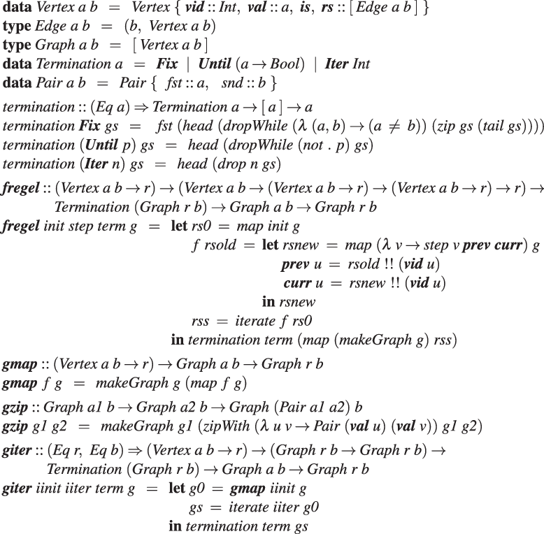
Fig. 12. Haskell implementation of Fregel.
The second-order graph function
fregel
takes as its arguments an initialization function, a step function, a termination point, and an input graph and returns the resultant graph of its computation. As explained in Section 4.2, the definition of
fregel
here differs somewhat from that of
 ${\mathit{vcModel}}$
, because it has to implement the memorization mechanism. It does this by using two lists of computation results for all vertices, which are accessed via the vertex identifiers.
${\mathit{vcModel}}$
, because it has to implement the memorization mechanism. It does this by using two lists of computation results for all vertices, which are accessed via the vertex identifiers.
Function
gmap
applies a given function to every vertex in the target graph and returns a new graph with the same shape in which each vertex has the application result. This is simply defined in terms of
 ${\mathit{makeGraph}}$
, for which the definition was presented in Section 3.
${\mathit{makeGraph}}$
, for which the definition was presented in Section 3.
Function
gzip
is given two graphs of the same shape and returns a graph in which each vertex has a pair of values that correspond to those of the vertices of the two graphs. A pair is defined by the
 ${\mathit{Pair}}$
type with
${\mathit{Pair}}$
type with
 ${\mathit{\_fst}}$
and
${\mathit{\_fst}}$
and
 ${\mathit{\_snd}}$
fields. This function can also be defined in terms of
${\mathit{\_snd}}$
fields. This function can also be defined in terms of
 ${\mathit{makeGraph}}$
.
${\mathit{makeGraph}}$
.
Function
giter
is given four arguments: iinit, iiter,
 ${\mathit{term}}$
, and an input graph. It first applies
${\mathit{term}}$
, and an input graph. It first applies
 ${\boldsymbol{gmap}~iinit}$
to the input graph and then repeatedly applies iiter to the result to produce a list of graphs. Finally, it uses
${\boldsymbol{gmap}~iinit}$
to the input graph and then repeatedly applies iiter to the result to produce a list of graphs. Finally, it uses
 ${\mathit{term}}$
to terminate the iteration and obtain the final result. It can be defined by using a standard function,
${\mathit{term}}$
to terminate the iteration and obtain the final result. It can be defined by using a standard function,
 ${\mathit{iterate}}$
.
${\mathit{iterate}}$
.
6 Fregel compiler
This section describes the basic compilation flow of Fregel programs. Optimizations for coping with the apparent inefficiency problems described in Section 2.2 are described in Section 7.
6.1 Overview of Fregel compiler
The Fregel compiler is a source-to-source translator from a Fregel program to a program for a Pregel-like framework for vertex-centric graph processing. Currently, our target frameworks are Giraph, for which the programs are in Java, and Pregel+, for which the programs are in C++. The Fregel compiler is implemented in Haskell. Figure 13 presents the compilation flow of a Fregel program.
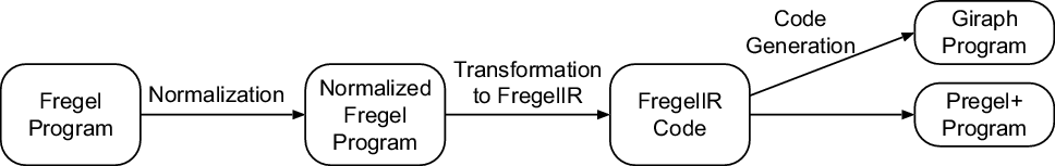
Fig. 13. Compilation flow of Fregel program.
First, a Fregel program is parsed into an abstract syntax tree (AST). Then the AST is transformed into another AST for a normalized Fregel program. Since ASTs are internal representations of Fregel programs, we show Fregel programs instead of their ASTs hereafter.
As we have seen in Sections 4.4 and 4.6, a Fregel program can contain multiple uses of second-order graph functions. We do not naively compile each second-order graph function into a Pregel computation, because each invocation of a Pregel computation may start up the Pregel system, which is costly. Instead, we normalize the AST for a Fregel program with (possibly) multiple uses of second-order graph functions into an equivalent one of the following form that uses fregel with Fix as the only use of a second-order graph function:
 \begin{equation*}\begin{array}{l}prog~g~~=~~\textbf{let}~\ldots~\textbf{in}~~\boldsymbol{fregel}~newInit~newStep~\boldsymbol{Fix}~g\end{array}\end{equation*}
We call this process and the resulting ASTs normalization and normalized ASTs, respectively. The normalized AST is transformed into an IR called FregelIR. FregelIR is a framework-independent representation in rather procedural style that is close to the target languages, Java (for Giraph) and C++ (for Pregel+). On the one hand, programs in these target languages have many common features such as control structures and styles of function (method) definitions. On the other hand, there are big differences that originate from the design of individual Pregel-like frameworks, such as how to define the compute function, how to exchange messages between vertices, and how to perform aggregations. Thus, we designed FregelIR as an appropriate abstraction layer that represents common features of the two frameworks and moreover absorbs the above-mentioned big differences.
Finally, Giraph or Pregel+ code is generated from a FregelIR representation depending on the option specified by the programmer. The Fregel compiler judges whether a given Fregel program uses reversed edges, rs , and records the judgment into the FregelIR representation of the program. If the program does not use rs , the compiler generates Giraph or Pregel+ code in which the vertices do not have a data structure for unnecessary reversed edges.
6.2 Normalization of Fregel programs
6.2.1 Simple example of normalization
Essentially, normalizing a Fregel program entails building a single-step function that emulates program execution. This step function is basically a phase transition machine. Before formerly describing the normalization algorithm, we explain the normalized program by using diameter in Figure 9 as an example. Recall that diameter contains two occurrences of fregel . The normalization results in a program of the following form:
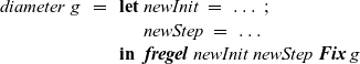 \begin{equation*}\begin{array}{l}diameter~g~~=~~\textbf{let}~newInit~=~\ldots~; \\\phantom{diameter~g~~=~~\textbf{let}~}newStep~=~\ldots \\\phantom{diameter~g~~=~~}\textbf{in}~~\boldsymbol{fregel}~newInit~newStep~\boldsymbol{Fix}~g\end{array}\end{equation*}
The program consists of a single fregel function. Its step function, that is, newStep, performs the essential computation in two phases followed by the termination phase. These two phases correspond to the two occurrences of fregel in the original program.
-
1. At the beginning of the first phase, the same initialization as that of ssspInit is performed. Then, the same computation as that of ssspStep for finding the shortest path length is repeatedly performed, and whether the computation has fallen into a steady state is detected. If a steady state is detected, the program moves on to the second phase.
-
2. At the beginning of the second phase, the same initialization as that of maxvInit is performed. During the second phase (except at the beginning), the same computation as that of maxvStep is performed and, similar to the first phase, whether the computation has fallen into a steady state is detected. If a steady state is detected, the program moves on to the termination phase.
Since newStep executes the computations of both fregel functions, it is necessary to combine the two records, namely SVal and MVal, into a single record. In addition, newStep has to determine what to execute in the current LSS. We thus let the combined record possess the current phase number and the current counter, that is, the elapsed clock, in the current phase. Thus, the combined record has the following definition:
 \begin{equation*}\begin{array}{l}\textbf{data}~ND~~=~~ND~\{\,phase :: \mathit{Int},~\mathit{counter} :: \mathit{Int},~datSVal :: SVal,~datMVal :: MVal\,\}\end{array}\end{equation*}
The initialization function, newInit, initializes this record appropriately.
Since newStep uses the combined record, record field accesses in the original program before normalization are replaced with the corresponding field accesses to the combined record as follows:
-
In
${ssspStep}: {\>\boldsymbol{prev}~{v}~.\wedge~{dist}~\longrightarrow~\boldsymbol{prev}~{v}~.\wedge~{datSVal}~.\wedge~dist}$
-
In
${maxvInit}: {\>\boldsymbol{val}~v~.\wedge~dist~\longrightarrow~\boldsymbol{prev}~{v}~.\wedge~{datSVal}~.\wedge~dist}$
-
In
${maxvStep}: {\>\boldsymbol{prev}~{v}~.\wedge~{maxv}~\longrightarrow~\boldsymbol{prev}~{v}~.\wedge~{datMVal}~.\wedge~maxv}$


Please note that since
 ${\boldsymbol{val}~v~.\wedge~dist}$
in maxvInit refers to the result of the first
fregel
in the original program, it corresponds to the dist field in SVal in the combined record at the previous clock. Thus, it is replaced with
${\boldsymbol{val}~v~.\wedge~dist}$
in maxvInit refers to the result of the first
fregel
in the original program, it corresponds to the dist field in SVal in the combined record at the previous clock. Thus, it is replaced with
 ${\boldsymbol{prev}~{v}~.\wedge~{datSVal}~.\wedge~dist}$
.
${\boldsymbol{prev}~{v}~.\wedge~{datSVal}~.\wedge~dist}$
.
The termination point of every
fregel
in the original program is examined explicitly in the newStep, because it advances the phase if the condition is satisfied. To this end, newStep uses an aggregation. Since
Fix
means a steady state, every vertex determines whether the previous and current values of the current phase’s computation are the same. For the first phase, previous and current values of vertex u are obtained by
 ${\boldsymbol{prev}~{u}~.\wedge~{datSVal}~.\wedge~dist}$
and
${\boldsymbol{prev}~{u}~.\wedge~{datSVal}~.\wedge~dist}$
and
 ${\boldsymbol{curr}~{u}~.\wedge~{datSVal}~.\wedge~dist}$
, respectively. Thus, when the current counter is positive, the result of the aggregation:
${\boldsymbol{curr}~{u}~.\wedge~{datSVal}~.\wedge~dist}$
, respectively. Thus, when the current counter is positive, the result of the aggregation:
 \begin{equation*}\begin{array}{l}\mathit{and}~[\>{\boldsymbol{prev}~{u}~.\wedge~{datSVal}~\mathbin{==}~\boldsymbol{curr}~{u}~.\wedge~{datSVal}}~|~{u} \leftarrow {g}{}\,]\end{array}\end{equation*}
represents whether the computation has reached a steady state, where g represents the target graph. If it has, newStep advances the phase field of the combined record. In addition,
 ${\mathit{counter}}$
is advanced every time LSS in the current phase is executed and is reset to zero when a new phase begins. The new values of phase and
${\mathit{counter}}$
is advanced every time LSS in the current phase is executed and is reset to zero when a new phase begins. The new values of phase and
 ${\mathit{counter}}$
are specified in the ND record returned by newStep.
${\mathit{counter}}$
are specified in the ND record returned by newStep.
Figure 14 presents the pseudocode of the normalized diameter. We suppose that the phase numbers of the first, second, and termination phases are one, two, and three, respectively. In addition, in the definition of newInit, defaultSVal and defaultMVal, respectively, represent appropriate default values of SVal and MVal for which the definitions are omitted. In the definition of newStep,
 ${d_1}$
is defined as the value of the datSVal field in the combined record at the next clock. Variable
${d_1}$
is defined as the value of the datSVal field in the combined record at the next clock. Variable
 ${e_1}$
is a Boolean value representing whether the first phase has reached the termination point. Variables
${e_1}$
is a Boolean value representing whether the first phase has reached the termination point. Variables
 ${d_2}$
and
${d_2}$
and
 ${e_2}$
are similarly defined.
${e_2}$
are similarly defined.
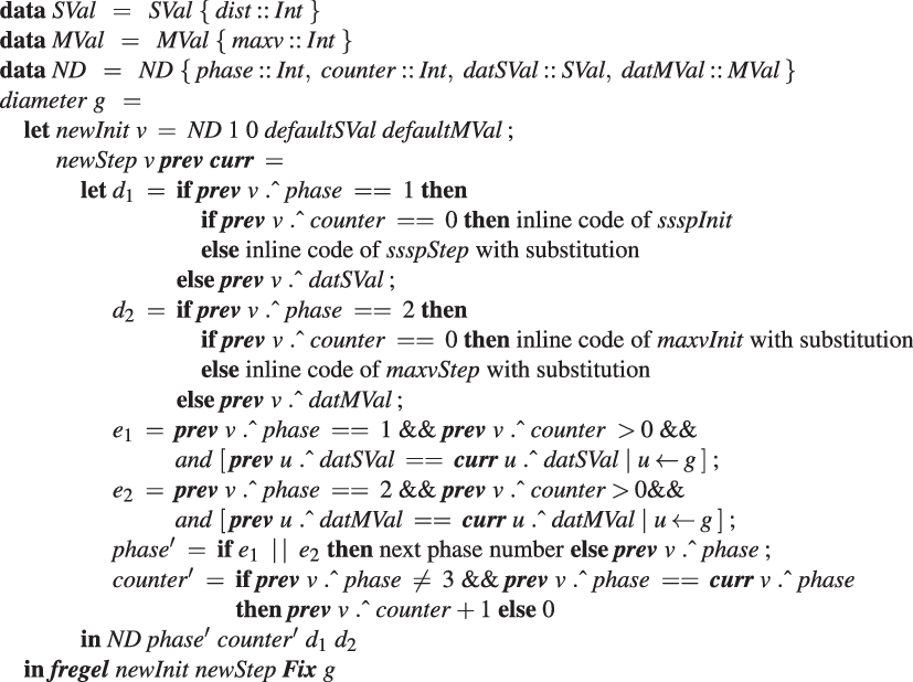
Fig. 14. Pseudocode of normalized Fregel program for calculating diameter.
6.2.2 Normalization algorithm
We assume that the following preprocessings have already been done on the target Fregel program. They are easily performed using standard techniques such as
 $\alpha$
-conversion.
$\alpha$
-conversion.
-
1. Bind every call of a second-order graph function to a distinct variable, which we call a graph variable.
-
2. Make variable names unique throughout the program, especially making sure that the variable name of the input graph given to the entire program is g as g is regarded as a special instance of a graph variable.
-
3. Make the function arguments of giter unique throughout the program. If two giter s uses the same function, the function should be duplicated with distinct names.
-
4. Inline user-defined variables and functions within step functions.
-
5. Infer types of subexpressions and make remaining type-variables monomorphic.
The normalization process consists of five steps.
Step 1: Enumerate phases
The first step is to enumerate each phase corresponding to a use of a second-order graph function. Given the first assumed preprocessing, this is essentially the same as enumerating graph variables except the one for the input graph. Thus, we use graph variables and phases interchangeably.
Let P be the set of graph variables except the input graph. Since
giter
s need special treatment later, we define a subset I of P, where
 $I = \{\,p \mid p \in P,~{\rm{p}} {\rm{binds}} \, {\rm{a}} \, {\boldsymbol{giter}} \, {\rm{result}}\,\}$
.
$I = \{\,p \mid p \in P,~{\rm{p}} {\rm{binds}} \, {\rm{a}} \, {\boldsymbol{giter}} \, {\rm{result}}\,\}$
.
For
 ${\mathit{scc}} $
in Figure 11, we have
${\mathit{scc}} $
in Figure 11, we have
 ${P = \{\,{gr,\,ga,\,gf,\,gb,\,gfb,\,g'}\,\}}$
and
${P = \{\,{gr,\,ga,\,gf,\,gb,\,gfb,\,g'}\,\}}$
and
 ${I = \{\,{gr}\,\}}$
.
${I = \{\,{gr}\,\}}$
.
Step 2: Define new record type
The next step is to define a new record type, ND, for use in the normalized program. We assume that
 ${P = \{\,p_1,\ldots,p_n\,\}}$
and
${P = \{\,p_1,\ldots,p_n\,\}}$
and
 ${I = \{\,p_{i_1},\ldots,p_{i_m}\,\}}$
 ${(m \le n,~i_1<i_2<\cdots<i_m)}$
and that
${(m \le n,~i_1<i_2<\cdots<i_m)}$
and that
 ${T_{p}}$
denotes the vertex type of a graph variable p. As stated in Section 6.2.1, we let ND possess the current phase number and the current counter in the current phase:
${T_{p}}$
denotes the vertex type of a graph variable p. As stated in Section 6.2.1, we let ND possess the current phase number and the current counter in the current phase:
 \begin{equation*}\begin{array}{l}\textbf{data}~ND~~=~~ND~\{\,phase :: \mathit{Int},\,\mathit{counter} :: \mathit{Int},\,d_{p_1} :: T_{p_1},\,\ldots,\,d_{p_n} :: T_{p_n},\\\phantom{\textbf{data}~ND~~=~~ND~\{\,}ictr_{p_{i_1}} :: \mathit{Int},\,\ldots,\,ictr_{p_{i_m}} :: \mathit{Int}\,\}\end{array}\end{equation*}
In the above definition of ND,
 ${dat_{p_j}}$
is used to hold the result of the computation of phase
${dat_{p_j}}$
is used to hold the result of the computation of phase
 ${p_j \in P}$
and
${p_j \in P}$
and
 ${ictr_{p_{i_j}}} $
is used to hold the number of iterations of the
giter
bound to
${ictr_{p_{i_j}}} $
is used to hold the number of iterations of the
giter
bound to
 ${p_{i_j} \in I}$
. The new record data for
${p_{i_j} \in I}$
. The new record data for
 ${\mathit{scc}}$
is shown at the head of Figure 16.
${\mathit{scc}}$
is shown at the head of Figure 16.
Step 3: Build code pieces for each phase
The new step function for the only
fregel
function in the normalized program needs two code pieces for every phase
 ${p \in P}$
: step function body
${p \in P}$
: step function body
 ${\textit{comp}_{p}}$
for implementing the computation in the phase and termination judgment expression
${\textit{comp}_{p}}$
for implementing the computation in the phase and termination judgment expression
 ${\mathit{texp}_{p}}$
for detecting the end of the computation in p.
${\mathit{texp}_{p}}$
for detecting the end of the computation in p.
During the building process of
 ${\textit{comp}_{p}}$
and
${\textit{comp}_{p}}$
and
 ${\mathit{texp}_{p}}$
,
prev
,
curr
, and
val
used in the original components must be replaced with suitable counterparts. To this end, we define two substitutions,
${\mathit{texp}_{p}}$
,
prev
,
curr
, and
val
used in the original components must be replaced with suitable counterparts. To this end, we define two substitutions,
 ${\sigma^1_{p}}$
and
${\sigma^1_{p}}$
and
 ${\sigma^2_{p'}}$
. The former defines the substitution of
${\sigma^2_{p'}}$
. The former defines the substitution of
 ${\boldsymbol{prev}~x}$
and
${\boldsymbol{prev}~x}$
and
 ${\boldsymbol{curr}~x}$
, while the latter defines the substitution of
${\boldsymbol{curr}~x}$
, while the latter defines the substitution of
 ${\boldsymbol{val}~x}$
. Their subscripts (p and p’) specify which member in the combined record ND is used in the substitution:
${\boldsymbol{val}~x}$
. Their subscripts (p and p’) specify which member in the combined record ND is used in the substitution:
 \begin{equation*}\begin{array}{l}\sigma^1_{p}~~=~~\{\,{\boldsymbol{prev}~x~~\mapsto~~\boldsymbol{prev}~{x}~.\wedge~{d_{p}},~~\boldsymbol{curr}~x~~\mapsto~~\boldsymbol{curr}~{x}~.\wedge~{d_{p}}}\,\}\\\sigma^2_{p'}~~=~~\textbf{if}~p'~\mathbin{==}~ g~\textbf{then}~\{\,{}\,\}~\textbf{else}~\{\,{\boldsymbol{val}~x~~\mapsto~~\boldsymbol{prev}~{x}~.\wedge~{d_{p'}}}\,\}\\\sigma_{p,p'}~~=~~\sigma^1_{p}~\cup~\sigma^2_{p'}\end{array}\end{equation*}
Both
 ${\textit{comp}_{p}}$
and
${\textit{comp}_{p}}$
and
 ${\mathit{texp}_{p}}$
depend on the second-order graph function for which the result is bound to the graph variable corresponding to p. In the following cases, we assume that v is the formal parameter for the vertex given to the new step function we are building.
${\mathit{texp}_{p}}$
depend on the second-order graph function for which the result is bound to the graph variable corresponding to p. In the following cases, we assume that v is the formal parameter for the vertex given to the new step function we are building.
Case 1:
 ${\>p~=~\boldsymbol{fregel}~init~step~\mathit{term}~p'}$
In this case,
 ${\textit{comp}_{p}}$
performs the computation of init at the beginning of the phase, that is, when
${\textit{comp}_{p}}$
performs the computation of init at the beginning of the phase, that is, when
 ${\mathit{counter}}$
is zero, or the computation of step afterward. Thus,
${\mathit{counter}}$
is zero, or the computation of step afterward. Thus,
 ${\textit{comp}_{p}}$
is defined as:
${\textit{comp}_{p}}$
is defined as:
 \begin{equation*}\begin{array}{l}\textit{comp}_{p}~~=~~\textbf{if}~\boldsymbol{prev}~{v}~.\wedge~{\mathit{counter}}~\mathbin{==}~ 0~\textbf{then}~\sigma_{p,p'}~(init~v)~\textbf{else}~\sigma_{p,p'}~(step~v~\boldsymbol{prev}~\boldsymbol{curr}),\end{array}\end{equation*}
where
 ${\sigma_{p,p'}~(init~v)}$
means applying substitution
${\sigma_{p,p'}~(init~v)}$
means applying substitution
 ${\sigma_{p,p'}}$
after inlining function application
${\sigma_{p,p'}}$
after inlining function application
 ${init~v}$
. Other applications of a substitution in the rest of this section are done in the same manner.
${init~v}$
. Other applications of a substitution in the rest of this section are done in the same manner.
Termination judgment expression
 ${\mathit{texp}_{p}}$
depends on the termination condition,
${\mathit{texp}_{p}}$
depends on the termination condition,
 ${\mathit{term}}$
.
${\mathit{term}}$
.
When
 ${\mathit{term}}$
is
${\mathit{term}}$
is
 ${\boldsymbol{Fix}}$
, judgment is done by checking whether the value of this phase remains unchanged on all vertices. Considering that this judgment is possible after running step at least once, we have the following definition of
${\boldsymbol{Fix}}$
, judgment is done by checking whether the value of this phase remains unchanged on all vertices. Considering that this judgment is possible after running step at least once, we have the following definition of
 ${\mathit{texp}_{p}}$
:
${\mathit{texp}_{p}}$
:
 \begin{equation*}\begin{array}{l}\mathit{texp}_{p}~~=~~\boldsymbol{prev}~{v}~.\wedge~{\mathit{counter}}~>~0~\&\&~and~[\>{\boldsymbol{prev}~{{u}}~.\wedge~{{d_p}}~\mathbin{==}~\boldsymbol{curr}~{{u}}~.\wedge~{d_p}}~|~{u} \leftarrow {p'}{}\,]\end{array}\end{equation*}
When term is
 ${\boldsymbol{Until}~(\lambda\,{p''} \rightarrow {e})}$
,
${\boldsymbol{Until}~(\lambda\,{p''} \rightarrow {e})}$
,
 ${\mathit{texp}_{p}}$
is defined as e with a suitable substitution applied:
${\mathit{texp}_{p}}$
is defined as e with a suitable substitution applied:
 \begin{equation*}\begin{array}{l}\mathit{texp}_{p}~~=~~\sigma^2_{p''}~(e)\end{array}\end{equation*}
When
 ${\mathit{term}}$
is
${\mathit{term}}$
is
 ${\boldsymbol{Iter}~k}$
, the judgment is done simply by checking the current counter:
${\boldsymbol{Iter}~k}$
, the judgment is done simply by checking the current counter:
 \begin{equation*}\begin{array}{l}\mathit{texp}_{p}~~=~~\boldsymbol{prev}~{v}~.\wedge~{\mathit{counter}}~\mathbin{==}~ k\end{array}\end{equation*}
Case 2:
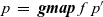 ${\>p~=~\boldsymbol{gmap}~f~p'}$
In this case,
 ${\textit{comp}_{p}}$
simply applies substitution
${\textit{comp}_{p}}$
simply applies substitution
 ${\sigma_{p,p'}}$
to the inlining result of
${\sigma_{p,p'}}$
to the inlining result of
 ${f~v}$
. Since
gmap
does not perform iterative computation,
${f~v}$
. Since
gmap
does not perform iterative computation,
 ${\mathit{texp}_{p}}$
is always true:
${\mathit{texp}_{p}}$
is always true:
 \begin{equation*}\begin{array}{l}\textit{comp}_{p}~~=~~\sigma_{p,p'}~(f~v)\\\mathit{texp}_{p}~~=~~True\end{array}\end{equation*}
Case 3:
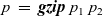 ${\>p~=~\boldsymbol{gzip}~p_1~p_2}$
In this case,
 ${\textit{comp}_{p}}$
pairs up the components corresponding to graph variables
${\textit{comp}_{p}}$
pairs up the components corresponding to graph variables
 ${p_1}$
and
${p_1}$
and
 ${p_2}$
. Similar to Case 2,
${p_2}$
. Similar to Case 2,
 ${\mathit{texp}_{p}}$
is always true:
${\mathit{texp}_{p}}$
is always true:
 \begin{equation*}\begin{array}{l}\textit{comp}_{p}~~=~~Pair~(\boldsymbol{prev}~{v}~.\wedge~{d_{p_1}})~(pv{v}{d_{p_2}})\\\mathit{texp}_{p}~~=~~True\end{array}\end{equation*}
Case 4:
 ${\>p~=~\boldsymbol{giter}~iinit~iiter~\mathit{term}~p'}$
In this case,
 ${\textit{comp}_{p}}$
performs initialization by iinit for the first time, that is, when
${\textit{comp}_{p}}$
performs initialization by iinit for the first time, that is, when
 ${ictr_{p}}$
is 0. Note that
${ictr_{p}}$
is 0. Note that
 ${ictr_{p}}$
holds the number of iterations of the corresponding
giter
. Otherwise, since the computation of
${ictr_{p}}$
holds the number of iterations of the corresponding
giter
. Otherwise, since the computation of
 ${\textit{comp}_{p}}$
has already been done by iiter,
${\textit{comp}_{p}}$
has already been done by iiter,
 ${\textit{comp}_{p}}$
can simply obtain the result of iiter by
${\textit{comp}_{p}}$
can simply obtain the result of iiter by
 ${d_{p''}}$
, where p” is the output graph of iiter:
${d_{p''}}$
, where p” is the output graph of iiter:
 \begin{equation*}\begin{array}{l}\textit{comp}_{p}~~=~~ \textbf{if}~{\boldsymbol{prev}~{v}~.\wedge~{ictr_p}~\mathbin{==}~ 0}~\textbf{then}~{\sigma_{p,p'}(iinit~v)}~\textbf{else} {\boldsymbol{prev}~{v}~.\wedge~{d_{p''}}}\end{array}\end{equation*}
Similar to Case 1, termination judgment expression
 ${\mathit{texp}_{p}}$
depends on termination condition
${\mathit{texp}_{p}}$
depends on termination condition
 ${\mathit{term}}$
. The difference is that
${\mathit{term}}$
. The difference is that
 ${ictr_{p}}$
is used instead of
${ictr_{p}}$
is used instead of
 ${\mathit{counter}}$
for
giter
. Specifically, when term is
${\mathit{counter}}$
for
giter
. Specifically, when term is
 ${\boldsymbol{Fix}}$
,
${\boldsymbol{Fix}}$
,
 ${\mathit{texp}_p}$
is as follows:
${\mathit{texp}_p}$
is as follows:
 \begin{equation*}\begin{array}{l}\mathit{texp}_{p}~~=~~\boldsymbol{prev}~{v}~.\wedge~{ictr_p}>0~\&\&~and~[\>{\boldsymbol{prev}~{{u}}~.\wedge~{{d_p}}~\mathbin{==}~\boldsymbol{curr}~{{u}}~.\wedge~{d_p}}~|~{u} \leftarrow {p'}{}\,]\end{array}\end{equation*}
When term is
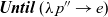 ${\boldsymbol{Until}~(\lambda\,{p''} \rightarrow {e})}$
,
${\boldsymbol{Until}~(\lambda\,{p''} \rightarrow {e})}$
,
 \begin{equation*}\begin{array}{l}\mathit{texp}_{p}~~=~~\sigma^2_{p''}~(e).\end{array}\end{equation*}
When
 ${\mathit{term}}$
is
${\mathit{term}}$
is
 ${\boldsymbol{Iter}~k}$
,
${\boldsymbol{Iter}~k}$
,
 \begin{equation*}\begin{array}{l}\mathit{texp}_{p}~~=~~\boldsymbol{prev}~{v}~.\wedge~{d_p}~\mathbin{==}~ k.\end{array}\end{equation*}
Step 4: Build a phase transition machine
Now we define a phase transition machine by using two functions.
One,
 ${\textit{next} :: P \rightarrow P}$
, is used to indicate which phase is to be executed next when the computation of the current phase terminates (i.e., when the termination judgment expression returns True.) This is defined by a topological sort determined by the dependencies of graph variables. For a program that uses
giter
, since the output graph of iiter is bound to the graph variable corresponding to the
giter
, this dependency also has to be taken into account.
${\textit{next} :: P \rightarrow P}$
, is used to indicate which phase is to be executed next when the computation of the current phase terminates (i.e., when the termination judgment expression returns True.) This is defined by a topological sort determined by the dependencies of graph variables. For a program that uses
giter
, since the output graph of iiter is bound to the graph variable corresponding to the
giter
, this dependency also has to be taken into account.
The other,
 ${\mathit{stay} :: P \to P}$
, is used to indicate which phase is to be executed to continue the computation in the current phase (i.e., when the termination judgment expression returns False.) Basically,
${\mathit{stay} :: P \to P}$
, is used to indicate which phase is to be executed to continue the computation in the current phase (i.e., when the termination judgment expression returns False.) Basically,
 ${\mathit{stay}~p = p}$
for most phases, but for a phase that corresponds to
giter
,
${\mathit{stay}~p = p}$
for most phases, but for a phase that corresponds to
giter
,
 ${\mathit{stay}}$
returns the entry phase of the iterative computation by the
giter
.
${\mathit{stay}}$
returns the entry phase of the iterative computation by the
giter
.
For example, graph variables of
 ${\mathit{scc}}$
have the following dependencies:
${\mathit{scc}}$
have the following dependencies:
-
${\mathit{gf}}$
and gb depend on
${\mathit{ga}}$
by
fregel
.
-
${\mathit{gf}b}$
depends on
${\mathit{gf}}$
and gb by
gzip
.
-
g’ depends on
${\mathit{gf}b}$
by
gmap
. -
gr depends on g’ because gr corresponds to giter and g’ is the output of sccIter.
-
${\mathit{ga}}$
depends on gr because
${\mathit{ga}}$
is the input graph of
giter
.


Thus, we can define
 ${\textit{next}(\mathit{ga}) = \mathit{gf}}$
,
${\textit{next}(\mathit{ga}) = \mathit{gf}}$
,
 ${\textit{next}(\mathit{gf}) = gb}$
,
${\textit{next}(\mathit{gf}) = gb}$
,
 ${\textit{next}(gb) = \mathit{gf}b}$
,
${\textit{next}(gb) = \mathit{gf}b}$
,
 ${\textit{next}(\mathit{gf}b) = g'}$
, and
${\textit{next}(\mathit{gf}b) = g'}$
, and
 ${\textit{next}(g') = gr}$
. It should be noted that we can swap
${\textit{next}(g') = gr}$
. It should be noted that we can swap
 ${\mathit{gf}}$
and gb in the above definition of
${\mathit{gf}}$
and gb in the above definition of
 ${\textit{next}}$
because there is no dependency between them. For
${\textit{next}}$
because there is no dependency between them. For
 ${\mathit{stay}}$
, we define
${\mathit{stay}}$
, we define
 ${\mathit{stay}(gr) = \mathit{ga}}$
because
${\mathit{stay}(gr) = \mathit{ga}}$
because
 ${\mathit{ga}}$
is the entry phase of
giter
, and
${\mathit{ga}}$
is the entry phase of
giter
, and
 ${\mathit{stay}(p) = p}$
for other phases.
${\mathit{stay}(p) = p}$
for other phases.
Step 5: Build a normalized program
A normalized program is built by using the components built so far. We assign a unique phase number (integer)
 ${\mathit{r}_p}$
to each phase p. We also introduce a special phase
${\mathit{r}_p}$
to each phase p. We also introduce a special phase
 ${p_e}$
and its phase number
${p_e}$
and its phase number
 ${\mathit{r}_{p_e}}$
to indicate the termination of the entire computation and let
${\mathit{r}_{p_e}}$
to indicate the termination of the entire computation and let
 ${\mathit{stay}(p_e) = p_e}$
and
${\mathit{stay}(p_e) = p_e}$
and
 ${\textit{next}(gr) = p_e}$
, where gr is the output graph variable in the original program.
${\textit{next}(gr) = p_e}$
, where gr is the output graph variable in the original program.
Figure 15 shows the template of a normalized Fregel program. The main part is the new step function, newStep, to emulate the original computation. When the current phase number obtained by
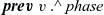 ${\boldsymbol{prev}~{v}~.\wedge~{phase}}$
is
${\boldsymbol{prev}~{v}~.\wedge~{phase}}$
is
 ${\mathit{r}_{p_j}}$
, it executes the step function body
${\mathit{r}_{p_j}}$
, it executes the step function body
 ${\textit{comp}_{p_j}}$
. The phase transition is controlled by the termination judgments,
${\textit{comp}_{p_j}}$
. The phase transition is controlled by the termination judgments,
 ${\mathit{texp}_{p_j}}$
, and the transition functions,
${\mathit{texp}_{p_j}}$
, and the transition functions,
 ${\textit{next}}$
and
${\textit{next}}$
and
 ${\mathit{stay}}$
. Note that newStep returns the same value as before once
${\mathit{stay}}$
. Note that newStep returns the same value as before once
 ${\boldsymbol{prev}~{v}~.\wedge~{phase}}$
becomes
${\boldsymbol{prev}~{v}~.\wedge~{phase}}$
becomes
 ${n_{p_e}}$
, because
${n_{p_e}}$
, because
 ${\mathit{stay}(p_e)}$
returns
${\mathit{stay}(p_e)}$
returns
 ${p_e}$
and
${p_e}$
and
 ${\mathit{counter}'}$
is always bound to 0. Thus, the computation terminates. The initialization function, newInit, simply initializes the current phase to
${\mathit{counter}'}$
is always bound to 0. Thus, the computation terminates. The initialization function, newInit, simply initializes the current phase to
 ${r_{p_1}}$
, counters (
${r_{p_1}}$
, counters (
 ${\mathit{counter}}$
,
${\mathit{counter}}$
,
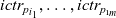 ${ictr_{p_{i_1}}, \ldots, ictr_{p_{1_m}}}$
) to 0, and other members in ND to their default values,
${ictr_{p_{i_1}}, \ldots, ictr_{p_{1_m}}}$
) to 0, and other members in ND to their default values,
 ${\mathit{defval}_{p_{i_j}}}$
.
${\mathit{defval}_{p_{i_j}}}$
.
Figure 16 presents the normalized Fregel program for
 ${\mathit{scc}}$
in Figure 11.
${\mathit{scc}}$
in Figure 11.
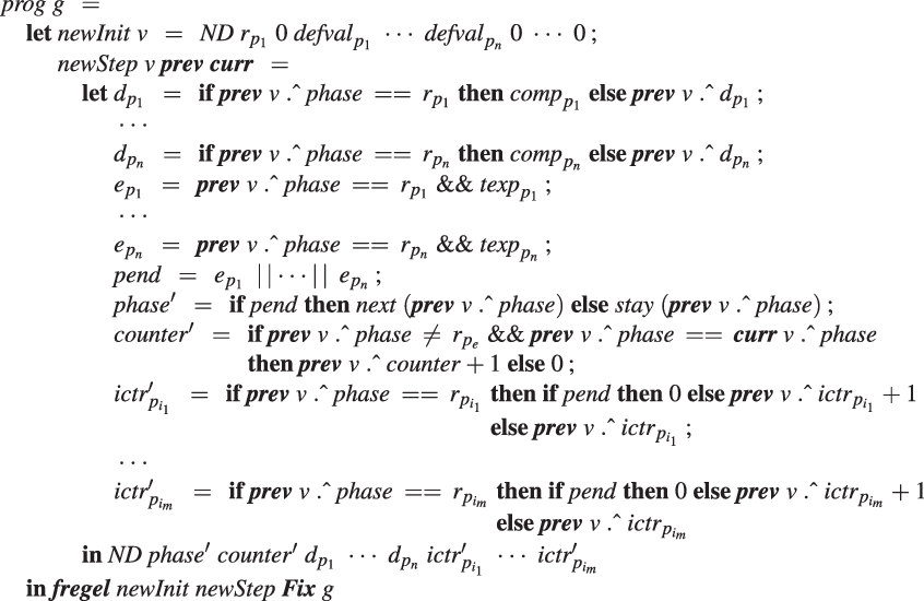
Fig. 15. Template of normalized Fregel program.

Fig. 16. Normalized Fregel program for scc.
6.2.3 Simple optimization in normalization process
For brevity, the transformation explained so far did not take the efficiency of the normalized program into account and introduced much redundancy. Standard optimizations such as inlining and simplification can reduce redundancy. For example, on the right-hand side of
 ${d_{g'}}$
of the normalized program in Figure 16, the redundant pair introduced by
gzip
can be eliminated by replacing
${d_{g'}}$
of the normalized program in Figure 16, the redundant pair introduced by
gzip
can be eliminated by replacing
 ${\boldsymbol{prev}~{v}~.\wedge~{d_\mathit{gf}b}~.\wedge~\mathit{\_fst}}$
and
${\boldsymbol{prev}~{v}~.\wedge~{d_\mathit{gf}b}~.\wedge~\mathit{\_fst}}$
and
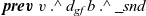 ${\boldsymbol{prev}~{v}~.\wedge~{d_\mathit{gf}b}~.\wedge~\mathit{\_snd}}$
with
${\boldsymbol{prev}~{v}~.\wedge~{d_\mathit{gf}b}~.\wedge~\mathit{\_snd}}$
with
 ${\boldsymbol{prev}~{v}~.\wedge~{d_\mathit{gf}}}$
and
${\boldsymbol{prev}~{v}~.\wedge~{d_\mathit{gf}}}$
and
 ${\boldsymbol{prev}~{v}~.\wedge~{d_gb}}$
, respectively. This simple optimization has been implemented in the normalization process.
${\boldsymbol{prev}~{v}~.\wedge~{d_gb}}$
, respectively. This simple optimization has been implemented in the normalization process.
6.3 Transforming normalized Fregel into FregelIR
6.3.1 Design of FregelIR
FregelIR is specialized to express Fregel programs. It bridges the gap between the functional style of Fregel programs and the imperative style of programs in the Giraph and Pregel+ frameworks. To this end, we designed FregelIR as a state transition machine with two key features. First, every phase in a normalized Fregel program is further split into subphases, each of which corresponds to a superstep in Pregel. As a result, a phase that performs communications including aggregations necessarily consists of multiple subphases. Each state is a pair of a phase and its subphase. Second, computation is imperative in a state where processing order is important. This makes generating Java and C++ programs from a FregelIR representation a straightforward process.
Figures 17 and 18 present simplified type definitions of FregelIR in Haskell.

Fig. 17. Simplified type definitions of FregelIR in Haskell.

Fig. 18. Simplified type definitions of FregelIR in Haskell, continued.
Type IRProg is the top-level representation for the entire program. It consists of datatypes used in phases, datatypes for vertices, edges, messages and aggregators, and IRCompute data that represents the computation. Each datatype has a name and members; IRVertexStruct has additional members for phase and subphase, and IRAggStruct has information about the aggregation operator for every aggregator. Type IRCompute is essentially a list of IRComputeProcess’es. Each IRComputeProcess represents the computation for its corresponding state with the following information:
-
state, that is, a pair of a phase and subphase,
-
local variables,
-
a block for the computation including receiving messages,
-
conditions for state transitions and next states, and
-
a block for sending messages to neighbors.
A block consists of statements represented in
 ${\mathit{IRStmt}}$
form, which has enough levels of abstraction to absorb the differences between frameworks. FregelIR contains minimum functionalities for expressing programs obtained from Fregel programs. For example, it does not have a structure corresponding to a general-purpose while-loop, because while-loops are unnecessary for transformed framework code.
${\mathit{IRStmt}}$
form, which has enough levels of abstraction to absorb the differences between frameworks. FregelIR contains minimum functionalities for expressing programs obtained from Fregel programs. For example, it does not have a structure corresponding to a general-purpose while-loop, because while-loops are unnecessary for transformed framework code.
We next explain the abstraction of FregelIR by using an example of the all-reachability problem, for which a program was presented in Figure 8. In the Fregel program, each vertex collects Boolean values sent from neighboring vertices by using a comprehension and takes their “or” value. This part is represented as the following type
 ${\mathit{IRStmt}}$
data:
${\mathit{IRStmt}}$
data:
 \begin{equation*}\begin{array}{l}IRStmtMsg~(IRVarLocal~(``agg",~irBool))~IRAggOr~(IRMVal~(``agg",~irBool))\end{array}\end{equation*}
Here,
 ${``agg"}$
is a local variable name to which the result is assigned. The same name is also used as the member name in the message structure. IRAggOr represents the disjunction operation used in combining received data, and irBool represents the Boolean type. This representation is abstract enough to express the computation in a framework-independent manner. From this IRStmtMsg structure, the following Java code for Giraph is generated, where MsgData is the typename for messages:
${``agg"}$
is a local variable name to which the result is assigned. The same name is also used as the member name in the message structure. IRAggOr represents the disjunction operation used in combining received data, and irBool represents the Boolean type. This representation is abstract enough to express the computation in a framework-independent manner. From this IRStmtMsg structure, the following Java code for Giraph is generated, where MsgData is the typename for messages:
agg = false;
for (MsgData msg : messages) agg = (agg || (msg.agg).get());
For Pregel+, the following C++ code is generated. Here, messages is a vector for messages incoming to the vertex:
agg = false;
for (int i = 0; i < messages.size(); i++)
agg = (agg || messages[i].agg_X425);
Note that in the above
 ${\mathit{IRStmt}}$
data, there is no explicit description of iterating over messages or of obtaining a Boolean value from each message.
${\mathit{IRStmt}}$
data, there is no explicit description of iterating over messages or of obtaining a Boolean value from each message.
6.3.2 Generating FregelIR
Through normalization, a Fregel program is transformed into a program that contains a single fregel function. However, there remain three essential differences between a normalized Fregel program and FregelIR code:
-
A normalized Fregel program is functional, while FregelIR code is imperative.
-
A normalized Fregel program describes an LSS, while FregelIR code is composed of supersteps in the Pregel sense.
-
A normalized Fregel program describes communications, that is, message exchanges between vertices and aggregations, based on comprehensions and values of other vertices found in a look-up table. In contrast, FregelIR code explicitly describes these communications.
For generating imperative FregelIR code, the FregelIR generator identifies the dependencies of let-bound variables and reorders computation of values for these variables so as not to refer to not-yet-computed values.
For every phase p, it is necessary to split the LSS composed by the step function body
 ${\textit{comp}_p}$
and termination judgment
${\textit{comp}_p}$
and termination judgment
 ${\mathit{texp}_p}$
into multiple supersteps at the points where communications occur. Each superstep is referred to as a subphase. As a concrete example, consider the generation of FregelIR code from the normalized
${\mathit{texp}_p}$
into multiple supersteps at the points where communications occur. Each superstep is referred to as a subphase. As a concrete example, consider the generation of FregelIR code from the normalized
 ${\mathit{scc}}$
program in Figure 16.
${\mathit{scc}}$
program in Figure 16.
In the expression bound to
 ${d_\mathit{gf}}$
, communications between adjacent vertices are performed using the following comprehension:
${d_\mathit{gf}}$
, communications between adjacent vertices are performed using the following comprehension:
 \begin{equation*}\begin{array}{l}minimum~[\>{\boldsymbol{prev}~{u}~.\wedge~{d_\mathit{gf}}~.\wedge~minv}~|~{(e,u)} \leftarrow {\boldsymbol{is}~v}{,~\boldsymbol{prev}~{u}~.\wedge~{d_\mathit{gf}}~.\wedge~notf}\,]\end{array}\end{equation*}
FregelIR code for this comprehension uses IRStmtSendN to send the minv value and then transits to the next subphase. From every IRStmtSendN, an appropriate code that uses a message-sending API for the target framework (Giraph or Pregel+) is generated. In the next subphase, the FregelIR code gathers the messages sent from neighbors in the previous subphase by using IRStmtMsg.
Similarly, an aggregation for termination detection can be found in the expression bound to
 ${e_\mathit{gf}}$
:
${e_\mathit{gf}}$
:
 \begin{equation*}\begin{array}{l}\mathit{and}~[\>{\boldsymbol{prev}~{u}~.\wedge~{d_\mathit{gf}}~\mathbin{==}~\boldsymbol{curr}~{u}~.\wedge~{d_\mathit{gf}}}~|~{u} \leftarrow {g}{}\,]\end{array}\end{equation*}
FregelIR code for this aggregation submits the result of equality test by using IRStmtAggr and then transits to the next subphase. The code receives the submitted values and combines them by the and function using IRAggr in the next subphase.
On the basis of the split subphases, FregelIR code is generated as a state transition machine. In the termination detection of each phase, if termination of the computation at the current phase is detected, the execution state at the next superstep is set to the entrance subphase of the next phase. Otherwise, it is set to the beginning of the iteration of the current phase.
By splitting a phase into multiple subphases, local (non-vertex) variables might be used over successive subphases, that is, supersteps. Such variables should be moved as member variables in the data structure held by each vertex.
6.4 Generating framework programs from FregelIR
From an IRProg structure for the entire program in PregeIR, a program for the target framework is generated. For every datatype in IRProg, a class (for Giraph) or a struct (for Pregel+) is defined. The target framework may require members that are not explicitly described in FregelIR, and such members are automatically added. For example, Pregel+ requires that the vertex struct has a vector of outgoing edges.
The compute function is built from IRComputeProcess datatypes, each of which describes a computation for its corresponding state. The compute function at each vertex dispatches its execution on the basis of the current phase and subphase obtained from its vertex struct.
For generating framework-dependent code, we used Haskell’s type classes. To illustrate the basic idea, we describe the generation of framework code for the following IRStmtMsg structure, which was presented in Section 6.3.1:
 \begin{equation*}\begin{array}{l}IRStmtMsg~(IRVarLocal~(``agg",~irBool))~IRAggOr~(IRMVal~(``agg",~irBool))\end{array}\end{equation*}
To enable framework-dependent code generation, we define a type class called PregelGenerator (Figure 19(a)). This type class is a collection of function and variable definitions used for generating framework-dependent code. For each framework, an instance of PregelGenerator is defined: GiraphGenerator for Giraph and PregelPlusGenerator for Pregel+.
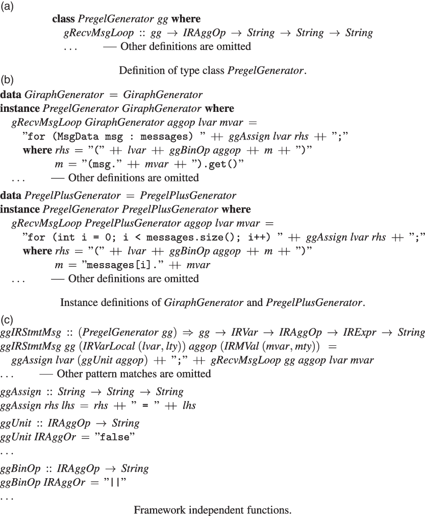
Fig. 19. Generating framework dependent code.
For the above example of IRStmtMsg, we generate framework code using ggIRStmtMsg, for which the definition is presented in Figure 19(c). Framework code consists of an initialization of the destination variable generated by ggAssign and a loop generated by gRecvMsgLoop, which successively takes a delivered message and performs a value-combining operation. In this code, since the loop structure is framework-dependent, PregelGenerator requires every instance to define gRecvMsgLoop, which generates a code fragment for the loop structure. Thus, GiraphGenerator and PregelPlusGenerator define gRecvMsgLoop so as to return a string containing a suitable for-statement (Figure 19(c)).
We do not convert the IR into the AST of the target language (Java or C++). This is because the IR itself is sufficiently low-level to enable program strings of the target language to be directly generated from the IR without going through an AST.
We defined every function that generates framework-dependent code to take an instance of PregelGenerator type class as its argument. By defining a suitable instance in this way, parts of the Fregel compiler for framework-dependent code generation can be packaged within the instance definition.
7 Code optimization
At this point, we have introduced the Fregel programming language and its basic compilation. Although this approach facilitates the development of runnable graph processing programs, as discussed in Section 2.1, it is still difficult to achieve efficiency. Natural programs tend to be slow.
To see the problem, recall the programs for the all-reachability problem (reAll) shown in Figure 8 and the single-source shortest path problem (sssp), which is the first half of the diameter problem in Figure 9. We use these two problems as running examples of the optimizations newly proposed in this section.
These two programs are based on the following algorithm:
-
First, the source vertex is assigned True (reAll) or 0 (sssp), and the other vertices are assigned False (reAll) or
${\infty}$
(sssp). For reAll, this value is the flag indicating whether each vertex is reachable or not at the current LSS. For sssp, this value is the tentative distance from the source vertex to each vertex at the current LSS. -
Then, each vertex sends the flag (reAll) or tentative distance (sssp) to its neighbors and updates its value if it receives True (reAll) or a shorter distance (sssp).
-
The second step is repeated until all vertex values are no longer changed.

While these programs are clear and reasonable, they also suffer from the following inefficiency problems discussed in Section 2.1. Some communications are apparently unnecessary (it is sufficient to process only those vertices for which values are updated), and global barrier synchronization for every superstep may bring overhead. Moreover, for sssp, there is an additional source of inefficiency: the algorithm is essentially the Bellman–Ford algorithm, for which the time complexity is
 $\mathrm{O}(n^2)$
, where n is the size of the graph, and processing near-source vertices prior to distant ones as in Dijkstra’s algorithm may reduce the amount of work to possibly
$\mathrm{O}(n^2)$
, where n is the size of the graph, and processing near-source vertices prior to distant ones as in Dijkstra’s algorithm may reduce the amount of work to possibly
 $\mathrm{O}(n \log n)$
.
$\mathrm{O}(n \log n)$
.
We developed a method for automatically removing these inefficiencies that incorporates four optimizations:
-
Eliminate unnecessary communications. (Section 7.2)
-
Inactivate vertices that do not need to be processed. (Section 7.3)
-
Remove barrier synchronization, thereby enabling asynchronous execution. (Section 7.4)
-
Introduce priorities for processing vertices. (Section 7.5)
These optimizations can be implemented by focusing on specific program patterns (Kato & Iwasaki Reference Kato and Iwasaki2019), but this ad hoc approach is sensitive to the program details. Our proposed method is based on a more robust approach that uses constraint solvers for identifying possible optimizations. We discuss the use of two constraint solving methods: quantifier elimination (QE) (Caviness & Johnson Reference Caviness and Johnson1998) and satisfiability modulo theories (SMT) (de Moura & BjØ rner Reference de Moura and BjØrner2011). The former enables the use of arbitrary quantifier nesting and can generate the program fragments that are necessary for the optimizations. Therefore, it is suitable for formalizing optimizations. However, it is somewhat impractical because of its high computational cost. We thus use SMT solvers as a practical implementation method that captures typical cases.
The first two optimizations listed above were implemented in the Fregel compiler. Implementation of the other two is left for future work because they need a graph processing framework that supports asynchronous execution. Nevertheless, we discuss them here in consideration of the possibility that they may be lead to further optimizations.
7.1 Target programs for optimization
The targets for the optimizations are programs written using the
 ${\boldsymbol{fregel}}$
function. We refer to its second parameter (a step function) as fStep and assume that it is written in the form shown in Figure 20. In the program,
${\boldsymbol{fregel}}$
function. We refer to its second parameter (a step function) as fStep and assume that it is written in the form shown in Figure 20. In the program,
 ${f_i}$
,
${f_i}$
,
 ${p_i}$
, and
${p_i}$
, and
 ${\oplus_i}$
 ${(1\leq i \leq n)}$
, respectively, represent computation over each neighbor’s value, the condition showing the necessity of sending the value, and the operator used for combining received values. Here, for convenience,
${(1\leq i \leq n)}$
, respectively, represent computation over each neighbor’s value, the condition showing the necessity of sending the value, and the operator used for combining received values. Here, for convenience,
 $\langle{aggOp}\rangle$
in the Fregel’s aggregation syntax (Figure 7) is represented by its commutative and associative binary operator
$\langle{aggOp}\rangle$
in the Fregel’s aggregation syntax (Figure 7) is represented by its commutative and associative binary operator
 $\oplus_i$
. For example, the aggregation operation “sum” is represented by its binary operator “+”. Function g denotes the calculation of the new value of a vertex. For simplicity, we assume the termination condition is
$\oplus_i$
. For example, the aggregation operation “sum” is represented by its binary operator “+”. Function g denotes the calculation of the new value of a vertex. For simplicity, we assume the termination condition is
 ${\boldsymbol{Fix}}$
, and only the
${\boldsymbol{Fix}}$
, and only the
 ${\boldsymbol{is}}$
function is used as a generator. We discuss these limitations in Section 7.6.
${\boldsymbol{is}}$
function is used as a generator. We discuss these limitations in Section 7.6.

Fig. 20. Target program for optimization.
The fStep corresponds to reStep for the reAll problem and ssspStep for the sssp problem, as presented in Table 1.
Table 1. Step functions for all-reachability and sssp problems

We use
 $\bar{\textit{u}}$
and
$\bar{\textit{u}}$
and
 $\bar{\bar{\textit{u}}}$
for the following meanings in this section:
$\bar{\bar{\textit{u}}}$
for the following meanings in this section:
-
$\bar{\textit{u}}$
denotes the current value of vertex u, and
-
$\bar{\bar{\textit{u}}}$
denotes the previous value of vertex u.


7.2 Eliminating unnecessary communications
Since accesses to a neighbor’s information are compiled to message exchange, modifying the condition
 ${p_k}$
and thereby avoiding unnecessary accesses reduces the amount of communication. In the following discussion, we focus on reducing communications caused by the computation of
${p_k}$
and thereby avoiding unnecessary accesses reduces the amount of communication. In the following discussion, we focus on reducing communications caused by the computation of
 ${c_k}$
. Our strategy is to formalize the situation in which optimization is possible and then to use constraint solvers to implement the optimization.
${c_k}$
. Our strategy is to formalize the situation in which optimization is possible and then to use constraint solvers to implement the optimization.
7.2.1 Formulation
Consider formulating the necessity of sending
 ${\bar{\textit{u}}}$
to neighboring vertices. The following property naturally formulates the situation in which the sending of
${\bar{\textit{u}}}$
to neighboring vertices. The following property naturally formulates the situation in which the sending of
 ${\bar{\textit{u}}}$
does not affect computation on the destination vertex:
${\bar{\textit{u}}}$
does not affect computation on the destination vertex:
 \begin{equation}\begin{array}{l}\forall~\mathit{pv},~e,~c_1,~\ldots,~c_n~.~\\g(\mathit{pv},~c_1,~\ldots,~c_n)~=~g(\mathit{pv},~c_1,~\ldots,~c_{k-1},~c_k\,\oplus_k\,f_k(e,~\bar{\textit{u}}),~c_{k+1},~\ldots,~c_n)\end{array}\end{equation}
For reStep, Property (7.1) is instantiated as:
 \begin{equation*}\begin{array}{l}\forall~\mathit{pv},~c~.~RVal~(\mathit{pv}~.\wedge~rch~\mid\mid~c)~=~RVal~(\mathit{pv}~.\wedge~rch~\mid\mid~(c~\mid\mid~\bar{\textit{u}}~.\wedge~rch)).\end{array}\end{equation*}
This is equivalent to
 ${\bar{\textit{u}}~.\wedge~rch~=~False}$
. It means that a vertex can skip message sending if its rch value is False.
${\bar{\textit{u}}~.\wedge~rch~=~False}$
. It means that a vertex can skip message sending if its rch value is False.
For ssspStep, Property (7.1) is instantiated as:
 \begin{equation*}\begin{array}{l}\forall~\mathit{pv},~e,~c~.~SVal~(\mathit{pv}~.\wedge~dist~`\mathit{min}`~c)~=~SVal~(\mathit{pv}~.\wedge~dist~`\mathit{min}`~(c~`\mathit{min}`~(\bar{\textit{u}}~.\wedge~dist + e))).\end{array}\end{equation*}
This is equivalent to
 ${\bar{\textit{u}}~.\wedge~dist~=~\infty}$
, which means that a vertex can skip message sending if its dist value is infinity.
${\bar{\textit{u}}~.\wedge~dist~=~\infty}$
, which means that a vertex can skip message sending if its dist value is infinity.
This property avoids the sending of apparently useless messages, a solution for the first inefficiency problem described above. Note that the “value of useless” derived from Property (7.1) is the unit value of
 ${\oplus_k}$
: False for
${\oplus_k}$
: False for
 ${\mathit{or}}$
and
${\mathit{or}}$
and
 ${\infty}$
for
${\infty}$
for
 ${`\mathit{min}'}$
. We call optimization on the basis of this property “unit values elimination.”
${`\mathit{min}'}$
. We call optimization on the basis of this property “unit values elimination.”
For both reAll and sssp, even more message sending can be avoided. A vertex need not send a message if its rch (reAll) or dist (sssp) value is unchanged from the previous step. To capture this case, we need another formulation that takes the previous value into account. A vertex may be able to skip message sending if sufficient information had been sent at the previous step. The following formula captures this idea:
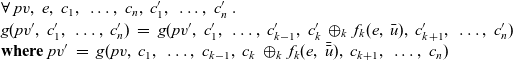 \begin{equation}\begin{array}{l}\forall~\mathit{pv},~e,~c_1,~\ldots,~c_n,~c'_1,~\ldots,~c'_n~.~\\g(\mathit{pv}',~c'_1,~\ldots,~c'_n)~=~g(\mathit{pv}',~c'_1,~\ldots,~c'_{k-1},~c'_k\,\oplus_k\,f_k(e,~\bar{\textit{u}}),~c'_{k+1},~\ldots,~c'_n)\\\textbf{where}~\mathit{pv}'~=~g(\mathit{pv},~c_1,~\ldots,~c_{k-1},~c_k\,\oplus_k\,f_k(e,~\bar{\bar{\textit{u}}}),~c_{k+1},~\ldots,~c_n)\end{array}\end{equation}
The necessity of
 ${\bar{\textit{u}}}$
is checked on the basis of the premise that the message-receiving vertex (which has value
${\bar{\textit{u}}}$
is checked on the basis of the premise that the message-receiving vertex (which has value
 ${\mathit{pv}'}$
) took into account the previous value
${\mathit{pv}'}$
) took into account the previous value
 ${\bar{\bar{\textit{u}}}}$
of the message-sending vertex. We call this optimization “redundant values elimination.”
${\bar{\bar{\textit{u}}}}$
of the message-sending vertex. We call this optimization “redundant values elimination.”
For reStep, Property (7.2) is instantiated to
 \begin{equation*}\begin{array}{l}\forall~\mathit{pv},~c,~c'~.~RVal~(\mathit{pv}'~.\wedge~rch~\mid\mid~c')=~RVal~(\mathit{pv}'~.\wedge~rch~\mid\mid~(c'~\mid\mid~\bar{\textit{u}}~.\wedge~rch))\\\phantom{\forall~\mathit{pv},~c,~c'~.~}\textbf{where}~\mathit{pv}'~=~RVal~(\mathit{pv}~.\wedge~rch~\mid\mid~(c~\mid\mid~\bar{\bar{\textit{u}}}~.\wedge~rch)).\end{array}\end{equation*}
This means that a vertex can skip communication when
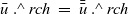 ${\bar{\textit{u}}~.\wedge~rch~=~\bar{\bar{\textit{u}}}~.\wedge~rch}$
, that is, the rch values of
${\bar{\textit{u}}~.\wedge~rch~=~\bar{\bar{\textit{u}}}~.\wedge~rch}$
, that is, the rch values of
 ${\bar{\textit{u}}}$
and
${\bar{\textit{u}}}$
and
 ${\bar{\bar{\textit{u}}}}$
are the same.
${\bar{\bar{\textit{u}}}}$
are the same.
Similarly for ssspStep, Property (7.2) is instantiated to
 \begin{equation*}\begin{array}{l}\forall~\mathit{pv},~e,~c,~c'~.~\\SVal~(\mathit{pv}'~.\wedge~dist~`\mathit{min}`~c')=~SVal~(\mathit{pv}'~.\wedge~dist~`\mathit{min}`~(c'~`\mathit{min}`~(\bar{\textit{u}}~.\wedge~dist+e)))\\\textbf{where}~\mathit{pv}'~=~SVal~(\mathit{pv}~.\wedge~dist~`\mathit{min}`~(c~`\mathit{min}`~(\bar{\bar{\textit{u}}}~.\wedge~dist+e))).\end{array}\end{equation*}
This is equivalent to
 ${\bar{\textit{u}}~.\wedge~dist~\geq~\bar{\bar{\textit{u}}}~.\wedge~dist\,}$
: a vertex can skip communication when the current dist value is not smaller than the previous one. Since the current dist value is never larger than the previous one, this is essentially equivalent to
${\bar{\textit{u}}~.\wedge~dist~\geq~\bar{\bar{\textit{u}}}~.\wedge~dist\,}$
: a vertex can skip communication when the current dist value is not smaller than the previous one. Since the current dist value is never larger than the previous one, this is essentially equivalent to
 ${\bar{\textit{u}}~.\wedge~dist~=~\bar{\bar{\textit{u}}}~.\wedge~dist}$
.
${\bar{\textit{u}}~.\wedge~dist~=~\bar{\bar{\textit{u}}}~.\wedge~dist}$
.
7.2.2 Remarks on implementation
We could implement this optimization by dynamically checking Properties (7.1) and (7.2) for each vertex. However, because these properties consist of quantifiers, their evaluation is likely impossible or very slow. To obtain efficient codes, we need a method for synthesizing a simple (especially quantifier-free) formula that is equivalent to (or expressing a sufficient condition of) the property. For this purpose, we can use constraint solvers.
QE translates a formula into a quantifier-free equivalent one. For example, it may translate
 $\forall x.~x^2 + ax + b \geq 0$
into
$\forall x.~x^2 + ax + b \geq 0$
into
 $4b - a^2 \geq 0$
. While QE is theoretically ideal for our purpose, QE solvers are impractical for three reasons. First, there are only a few formal systems for which QE procedures are known. Second, QE procedures are usually very slow. Third, current implementations of QE tend to be experimental. Nevertheless, it is worthwhile to formulate the optimizations as QE, because these problems may one day be solved.
$4b - a^2 \geq 0$
. While QE is theoretically ideal for our purpose, QE solvers are impractical for three reasons. First, there are only a few formal systems for which QE procedures are known. Second, QE procedures are usually very slow. Third, current implementations of QE tend to be experimental. Nevertheless, it is worthwhile to formulate the optimizations as QE, because these problems may one day be solved.
As a more practical implementation, we propose using SMT instead of QE. Given a closed formula consisting of only one kind of quantifier, SMT checks (i.e., does not translate) whether it is satisfiable. For example, it may answer “yes” for
 $\forall x,\,a.~x^2 + ax + a^2 \geq 0$
. Efficient SMT solvers have recently been developed and are now used in many applications.
$\forall x,\,a.~x^2 + ax + a^2 \geq 0$
. Efficient SMT solvers have recently been developed and are now used in many applications.
There are two problems in using SMT for checking Properties (7.1) and (7.2). They contain free variables,
 ${\bar{\textit{u}}}$
and
${\bar{\textit{u}}}$
and
 ${\bar{\bar{\textit{u}}}}$
, and moreover, SMT solvers are unable to synthesize a simple formula. To overcome these problems, we prepare templates of simple reasonable formulae, such as
${\bar{\bar{\textit{u}}}}$
, and moreover, SMT solvers are unable to synthesize a simple formula. To overcome these problems, we prepare templates of simple reasonable formulae, such as
 ${\bar{\textit{u}} = \infty}$
(e.g.,
${\bar{\textit{u}} = \infty}$
(e.g.,
 ${\bar{\textit{u}}~.\wedge~dist = \infty}$
) or
${\bar{\textit{u}}~.\wedge~dist = \infty}$
) or
 ${\bar{\textit{u}} = \bar{\bar{\textit{u}}}}$
. If the SMT solver guarantees that a template is a sufficient condition of these properties, we insert the negation of the template into
${\bar{\textit{u}} = \bar{\bar{\textit{u}}}}$
. If the SMT solver guarantees that a template is a sufficient condition of these properties, we insert the negation of the template into
 ${p_k}$
. The effectiveness of this approach relies on the generality of the template.
${p_k}$
. The effectiveness of this approach relies on the generality of the template.
The most common case that satisfies Property (7.1) is one in which the message value is the unit of
 ${\oplus_k}$
. Since Fregel’s syntax allows only a limited operator such as minimum and
${\oplus_k}$
. Since Fregel’s syntax allows only a limited operator such as minimum and
 ${\mathit{or}}$
as
${\mathit{or}}$
as
 $\langle{aggOp}\rangle$
, we can know the unit value of an
$\langle{aggOp}\rangle$
, we can know the unit value of an
 $\langle{{aggOp}}\rangle$
without using constraint solvers. However, if a user-defined combining operation were able to be specified as
$\langle{{aggOp}}\rangle$
without using constraint solvers. However, if a user-defined combining operation were able to be specified as
 $\langle{{aggOp}}\rangle$
, we would use an SMT solver to check whether one of the template values is the unit of the operation.
$\langle{{aggOp}}\rangle$
, we would use an SMT solver to check whether one of the template values is the unit of the operation.
For the case of Property (7.2), several templates can be considered. We believe that comparing values in
 ${\bar{\textit{u}}}$
and
${\bar{\textit{u}}}$
and
 ${\bar{\bar{\textit{u}}}}$
captures most practical cases.
${\bar{\bar{\textit{u}}}}$
captures most practical cases.
Considering sssp, for Property (7.1), we have already found that sending
 ${\infty}$
is unnecessary because it is the unit of
${\infty}$
is unnecessary because it is the unit of
 ${`\mathit{min}`}$
. For Property (7.2), we instruct an SMT solver to check the following formula:
${`\mathit{min}`}$
. For Property (7.2), we instruct an SMT solver to check the following formula:
 \begin{equation*}\begin{array}{l}\forall~\bar{\textit{u}},~\bar{\bar{\textit{u}}},~\mathit{pv},~e,~c,~c'~.~\\\bar{\textit{u}}~=~\bar{\bar{\textit{u}}}~\longrightarrow~SVal~(\mathit{pv}'~.\wedge~dist~`\mathit{min}`~c')=~SVal~(\mathit{pv}'~.\wedge~dist~`\mathit{min}`~(c'~`\mathit{min}`~(\bar{\textit{u}}~.\wedge~dist+e)))\\\phantom{\bar{\textit{u}}~=~\bar{\bar{\textit{u}}}~\longrightarrow~}\textbf{where}~\mathit{pv}'~=~SVal~(\mathit{pv}~.\wedge~dist~`\mathit{min}`~(c~`\mathit{min}`~(\bar{\bar{\textit{u}}}~.\wedge~dist+e))).\end{array}\end{equation*}
The solver verifies the condition. We thus modify the program as follows. We instruct each vertex to check and remember the truth of the template. Then, we modify
 ${p_1}$
so that it checks the remembered truth. Letting notChanged be the vertex variable for remembering the truth of the template, we modify ssspStep to a code that is essentially equivalent to the one presented in Figure 21.
${p_1}$
so that it checks the remembered truth. Letting notChanged be the vertex variable for remembering the truth of the template, we modify ssspStep to a code that is essentially equivalent to the one presented in Figure 21.

Fig. 21. sssp program for eliminating redundant communications.
7.3 Inactivating vertices
Next, we discuss inactivating vertices. A vertex u is inactivated if the following condition holds; unless the vertex receives a message, its value
 ${\bar{\textit{u}}}$
does not change and it need not send a message. The optimization condition is thus formalized as:
${\bar{\textit{u}}}$
does not change and it need not send a message. The optimization condition is thus formalized as:
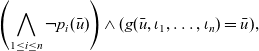 \begin{equation}\left(\bigwedge_{1 \leq i \leq n}\neg p_i(\bar{\textit{u}})\right) \wedge(g(\bar{\textit{u}},\iota_1,\ldots, \iota_n) = \bar{\textit{u}}),\end{equation}
where
 ${\iota_i~(1\leq i \leq n)}$
is the unit of
${\iota_i~(1\leq i \leq n)}$
is the unit of
 ${\oplus_i}$
and corresponds to the absence of messages. In Property (7.3), “
${\oplus_i}$
and corresponds to the absence of messages. In Property (7.3), “
 ${\neg p_i(\bar{\textit{u}})}$
” corresponds to the fact that the current vertex need not send a message for the i-th aggregation, and “
${\neg p_i(\bar{\textit{u}})}$
” corresponds to the fact that the current vertex need not send a message for the i-th aggregation, and “
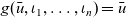 ${g(\bar{\textit{u}},\iota_1,\ldots, \iota_n) = \bar{\textit{u}}}$
” means that the vertex’s value is unchanged unless the vertex received a message. Since this property contains no quantifier, this optimization can be implemented without the use of a constraint solver. We call this optimization “vertices inactivation.”
${g(\bar{\textit{u}},\iota_1,\ldots, \iota_n) = \bar{\textit{u}}}$
” means that the vertex’s value is unchanged unless the vertex received a message. Since this property contains no quantifier, this optimization can be implemented without the use of a constraint solver. We call this optimization “vertices inactivation.”
For effective vertices inactivation, the predicate
 $p_i$
, which specifies the necessity of sending messages, should result in “false” as much as possible. Hence, vertices inactivation should be applied after communication reduction optimization described in Section 7.2.
$p_i$
, which specifies the necessity of sending messages, should result in “false” as much as possible. Hence, vertices inactivation should be applied after communication reduction optimization described in Section 7.2.
For sssp, Property (7.3) is instantiated to
 \begin{equation*}\begin{array}{l}\bar{\textit{u}}~.\wedge~notChanged~\wedge~(SVal~d'~(d'~~\mathbin{==}~~\bar{\textit{u}}~.\wedge~dist))~=~\bar{\textit{u}}~~\textbf{where}~d'~=~\bar{\textit{u}}~.\wedge~dist~`\mathit{min}`~\infty,\end{array}\end{equation*}
which is equivalent to
 ${\bar{\textit{u}}~.\wedge~notChanged}$
. In short, a vertex can be inactivated if its value is the same as before.
${\bar{\textit{u}}~.\wedge~notChanged}$
. In short, a vertex can be inactivated if its value is the same as before.
7.4 Removing barriers
Recall that the execution of Fregel is based on the BSP model. Each local computation is followed by barrier synchronization. Though this makes program behaviors deterministic and deadlock-free, barriers can make execution slower, especially when there are many computational nodes. For most graph algorithms including reAll and sssp for which asynchronous barrier-less execution and synchronous execution yield the same result, barrier synchronization is unnecessary.
The flexibility of asynchronous execution enables further optimizations such as vertex splitting (also known as vertex mirroring) (Yan et al. Reference Yan, Cheng, Lu and Ng2015; Verma et al. Reference Verma, Leslie, Shin and Gupta2017). Practical graphs often contain vertices that have too many edges, and such vertices form a bottleneck in vertex-centric computation. Vertex splitting resolves the bottleneck by splitting these vertices and distributing their edges among the computational nodes. With synchronous execution, vertex splitting requires an additional superstep to merge the messages sent to the split vertices. With asynchronous execution, an additional superstep is unnecessary because message delay does not matter. Another possible optimization is to repeatedly process vertices in the same computational node before sending messages to other nodes. This optimization is related to subgraph-centric (or neighborhood-centric) approaches (Tian et al. Reference Tian, Balmin, Corsten, Tatikonda and McPherson2013; Quamar et al. Reference Quamar, Deshpande and Lin2016) in which subgraphs rather than vertices are the target of parallel processing.
7.4.1 Formulation
We have developed a method that automatically guarantees equivalence between synchronous and asynchronous execution. We first present the following lemma.
Lemma 7.1. For functions h and h’ and a binary relation
 $\preceq$
, three conditions are assumed:
$\preceq$
, three conditions are assumed:
-
Monotonicity of h :
$\forall x,y.~(x \preceq y) \rightarrow (h(x) \preceq h(y))$
. -
Ordering of h and h ’:
$\forall x.~ (x \preceq h'(x)) \wedge (h'(x) \preceq h(x))$
. -
Antisymmetry of
$\preceq$
:
$\forall x,y.~ (x \preceq y \wedge y\preceq x) \rightarrow (x=y)$
.


Then,
 $h^*(x) = h^*(h'(x))$
holds for any x, where
$h^*(x) = h^*(h'(x))$
holds for any x, where
 $h^*$
is defined by
$h^*$
is defined by
 $h^*(x)~=~\mathbf{if}~h(x)=x~\mathbf{then}~x~\mathbf{else}~h^*(h(x))$
.
$h^*(x)~=~\mathbf{if}~h(x)=x~\mathbf{then}~x~\mathbf{else}~h^*(h(x))$
.
Proof. From the monotonicity and the ordering of h and h’, we have
 $x \preceq h'(x) \preceq h(x) \preceq h(h'(x))$
. Now let
$x \preceq h'(x) \preceq h(x) \preceq h(h'(x))$
. Now let
 $h^0(x) = x$
and
$h^0(x) = x$
and
 $h^n(x) = h^{n-1}(h(x))$
for
$h^n(x) = h^{n-1}(h(x))$
for
 $n > 1$
. By induction, we have
$n > 1$
. By induction, we have
 $h^n(x) \preceq h^n(h'(x)) \preceq h^{n+1}(x)$
for any n. When
$h^n(x) \preceq h^n(h'(x)) \preceq h^{n+1}(x)$
for any n. When
 $h^{*}(x)$
terminates, there exists an integer m such that
$h^{*}(x)$
terminates, there exists an integer m such that
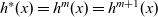 $h^{*}(x) = h^m(x) = h^{m+1}(x)$
. Then,
$h^{*}(x) = h^m(x) = h^{m+1}(x)$
. Then,
 $h^m(x) = h^m(h'(x)) = h^{m+1}(x)$
follows from the inequality mentioned above and the antisymmetry of
$h^m(x) = h^m(h'(x)) = h^{m+1}(x)$
follows from the inequality mentioned above and the antisymmetry of
 $\preceq$
, and hence
$\preceq$
, and hence
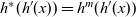 $h^{*}(h'(x)) = h^m(h'(x))$
. When
$h^{*}(h'(x)) = h^m(h'(x))$
. When
 $h^{*}(x)$
is non-terminating, so is
$h^{*}(x)$
is non-terminating, so is
 $h^{*}(h'(x))$
. We prove it by contradiction. Suppose
$h^{*}(h'(x))$
. We prove it by contradiction. Suppose
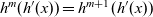 $h^m(h'(x)) = h^{m+1}(h'(x))$
for some m. Recall that
$h^m(h'(x)) = h^{m+1}(h'(x))$
for some m. Recall that
 $h^m(h'(x)) \preceq h^{m+1}(x) \preceq h^{m+1}(h'(x)) \preceq h^{m+2}(x) \preceq h^{m+2}(h'(x))$
holds. This inequality and
$h^m(h'(x)) \preceq h^{m+1}(x) \preceq h^{m+1}(h'(x)) \preceq h^{m+2}(x) \preceq h^{m+2}(h'(x))$
holds. This inequality and
 $h^m(h'(x)) = h^{m+1}(h'(x)) = h^{m+2}(h'(x))$
imply
$h^m(h'(x)) = h^{m+1}(h'(x)) = h^{m+2}(h'(x))$
imply
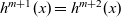 $h^{m+1}(x) = h^{m+2}(x)$
, which contradicts the non-termination of
$h^{m+1}(x) = h^{m+2}(x)$
, which contradicts the non-termination of
 $h^*(x)$
.
$h^*(x)$
.
We apply Lemma 7.1 as follows. We regard h as a complete one-step processing of the graph. Similarly, we regard h’ as a partial processing in which some vertices and messages are skipped. We regard asynchronous execution as a series of partial processings. Lemma 7.1 guarantees that a partial processing does not change the result; then, by induction, asynchronous execution does not change the result as well.
Lemma 7.1 requires an appropriate binary relation,
 $\preceq$
. From the ordering between h and h’, a natural candidate is comparison of the progress in computation:
$\preceq$
. From the ordering between h and h’, a natural candidate is comparison of the progress in computation:
 $g_1 \preceq g_2$
indicates that graph
$g_1 \preceq g_2$
indicates that graph
 $g_2$
can be obtained by processing computation from
$g_2$
can be obtained by processing computation from
 $g_1$
. Another requirement is bridging the gap between graph processing and vertex processing. While h, h’, and
$g_1$
. Another requirement is bridging the gap between graph processing and vertex processing. While h, h’, and
 $\preceq$
deal with graphs, we would like to consider vertex-processing functions. The following lemma bridges the gap. For simplicity, we assume that the fStep function contains only one access to a neighbor’s information by a combining operator
$\preceq$
deal with graphs, we would like to consider vertex-processing functions. The following lemma bridges the gap. For simplicity, we assume that the fStep function contains only one access to a neighbor’s information by a combining operator
 ${\oplus}$
.
${\oplus}$
.
Lemma 7.2. For fStep, let
 $\preceq$
be a binary relation defined by
$\preceq$
be a binary relation defined by
 $x \preceq y \iff (\exists m.~y = g(x,m))$
. Three conditions are assumed:
$x \preceq y \iff (\exists m.~y = g(x,m))$
. Three conditions are assumed:
-
$\forall x,m,m'.~ g(x,m \oplus m') = g(g(x,m), m')$
.
-
$\forall x,y.~ (x \preceq y \wedge y\preceq x) \rightarrow (x=y)$
.
-
$\forall x,y,z.~(x \preceq y) \rightarrow (g(z,x) \preceq g(z,y))$
.


Then,
 ${h_fStep}$
,
${h_fStep}$
,
 ${h'_fStep}$
, and
${h'_fStep}$
, and
 $\preceq_\mathsf{G}$
satisfy the premise of Lemma 7.1: the first two are respectively complete and partial one-step processing (here, “partial” means processing some of the vertices using some of the messages) over the graph by fStep and the last one compares graphs on the basis of vertex-wise comparison using
$\preceq_\mathsf{G}$
satisfy the premise of Lemma 7.1: the first two are respectively complete and partial one-step processing (here, “partial” means processing some of the vertices using some of the messages) over the graph by fStep and the last one compares graphs on the basis of vertex-wise comparison using
 $\preceq$
.
$\preceq$
.
Proof [proof sketch.] The first condition and the definition of
 $\preceq$
guarantee the ordering between
$\preceq$
guarantee the ordering between
 ${h_fStep}$
and
${h_fStep}$
and
 ${h'_fStep}$
. The antisymmetry of
${h'_fStep}$
. The antisymmetry of
 $\preceq_\mathsf{G}$
easily follows from the second condition. The third condition together with the first one and the commutativity of
$\preceq_\mathsf{G}$
easily follows from the second condition. The third condition together with the first one and the commutativity of
 ${\oplus}$
guarantees the monotonicity of
${\oplus}$
guarantees the monotonicity of
 ${h_reStep}$
.
${h_reStep}$
.
The first condition of Lemma 7.2 can be taken to mean that message delay is not harmful. This is a natural requirement for asynchronous execution.
For sssp, the definition of the relation
 $\preceq$
is instantiated as:
$\preceq$
is instantiated as:
 \begin{equation*}\begin{array}{l}x \preceq y \iff \exists w.~ x ~.\wedge~dist ~`\mathit{min}`~ w ~.\wedge~dist = y,\end{array}\end{equation*}
which is equivalent to
 ${x~.\wedge~dist~\geq~y~.\wedge~dist}$
. Therefore, confirming the three conditions is easy.
${x~.\wedge~dist~\geq~y~.\wedge~dist}$
. Therefore, confirming the three conditions is easy.
7.4.2 Remarks on Implementation
The first and second conditions can be checked using either QE or SMT. Note that the second is equivalent to
 ${\forall x,~m,~w\,.~(g(g(x,m),w) = x) \rightarrow (g(x,m) = x)}$
, where y is expressed as g(x,m). Since the definition of
${\forall x,~m,~w\,.~(g(g(x,m),w) = x) \rightarrow (g(x,m) = x)}$
, where y is expressed as g(x,m). Since the definition of
 $\preceq$
contains an existential quantifier, the third condition cannot be directly checked using SMT. When using an SMT solver, we may instead check the following sufficient condition:
$\preceq$
contains an existential quantifier, the third condition cannot be directly checked using SMT. When using an SMT solver, we may instead check the following sufficient condition:
 \begin{equation*}\begin{array}{l}\forall x,~y,~z\,.~(x \preceq y) \rightarrow (g(g(z,x),y) = g(z,y)).\end{array}\end{equation*}
This can be read to mean that the previous result, x, can be “overwritten” by the newer result, y. This is also natural in asynchronous execution.
7.5 Prioritized execution
Another interesting optimization that asynchronous execution enables is prioritized execution (Prountzos et al. Reference Prountzos, Manevich and Pingali2015; Cruz et al. Reference Cruz, Rocha and Goldstein2016; Liu et al., Reference Liu, Zhou, Gao and Fan2016). For example, in sssp, a prioritized execution may more intensively process vertices nearer the source, like Dijkstra’s algorithm.
Prioritized execution typically focuses on vertices for which the values are nearer the final outcome and thus likely contribute to the final outcome for other vertices. Therefore, it is natural to use
 $\preceq$
defined in Lemma 7.1, which essentially compares progress in computation, as a priority for processing vertices. For sssp,
$\preceq$
defined in Lemma 7.1, which essentially compares progress in computation, as a priority for processing vertices. For sssp,
 $\preceq$
is equivalent to
$\preceq$
is equivalent to
 $\geq$
and thus is a perfect candidate.
$\geq$
and thus is a perfect candidate.
However, there are two problems with using
 $\preceq$
for prioritized execution. First, since its definition contains an existential quantifier, it is essentially not executable unless QE is used. The other, more essential problem is that
$\preceq$
for prioritized execution. First, since its definition contains an existential quantifier, it is essentially not executable unless QE is used. The other, more essential problem is that
 $\preceq$
may not be a linear order. Nonlinear orders are less effective for prioritized execution and make it difficult to process vertices efficiently using priority queues. A practical solution to these problems is to check whether a known linear order,
$\preceq$
may not be a linear order. Nonlinear orders are less effective for prioritized execution and make it difficult to process vertices efficiently using priority queues. A practical solution to these problems is to check whether a known linear order,
 $\geq$
for example, is consistent with
$\geq$
for example, is consistent with
 $\preceq$
, that is,
$\preceq$
, that is,
 $\forall x,y.~(x \preceq y) \rightarrow (x \geq y)$
. If it is, the linear order can be used for prioritization. The condition can be checked by an SMT solver.
$\forall x,y.~(x \preceq y) \rightarrow (x \geq y)$
. If it is, the linear order can be used for prioritization. The condition can be checked by an SMT solver.
7.6 Limitations and generalization
We have assumed that information read from neighbors is expressed using the
 $\boldsymbol{is}$
generator. Use of other kinds of generators, including the one for expressing an aggregator, generally does not introduce any difficulty. We did not assume anything about communication except that the communication topology does not change during computation.
$\boldsymbol{is}$
generator. Use of other kinds of generators, including the one for expressing an aggregator, generally does not introduce any difficulty. We did not assume anything about communication except that the communication topology does not change during computation.
A notable exception is the case of vertex inactivation. Since the results of aggregation may change regardless of message arrival, if the k-th communication is an aggregator, the following condition should be checked instead of Property (7.3):
 \begin{equation*}\left(\bigwedge_{1 \leq i \leq n}\neg p_i(\bar{\textit{u}})\right) \wedge( \forall w_k.~g(\bar{\textit{u}},\iota_1,\ldots,w_k,\ldots, \iota_n) = \bar{\textit{u}}).\end{equation*}
Namely, the vertex value should not change regardless of the aggregator’s value if the vertex does not receive a message. Since it contains a quantifier, unless QE is used, an executable sufficient condition is needed. A natural candidate is the following condition:
 \begin{equation*}\forall \bar{\textit{u}}.~\left(\bigwedge_{1 \leq i \leq n}\neg p_i(\bar{\textit{u}})\right) \rightarrow( \forall w_k.~g(\bar{\textit{u}},\iota_1,\ldots,w_k,\ldots, \iota_n) = \bar{\textit{u}}).\end{equation*}
If it holds, a vertex having
 $\bar{\textit{u}}$
can be inactivated if
$\bar{\textit{u}}$
can be inactivated if
 $(\bigwedge_{1 \leq i \leq n}\neg p_i(\bar{\textit{u}}))$
holds. The condition can be checked using SMT.
$(\bigwedge_{1 \leq i \leq n}\neg p_i(\bar{\textit{u}}))$
holds. The condition can be checked using SMT.
We have considered only a certain form of programs. For example, termination conditions other than
 ${\boldsymbol{Fix}}$
and second-order graph functions other than
fregel
were neglected. This limitation is theoretically inconsequential. As discussed in Section 6.2, the Fregel compiler normalizes other forms of programs into the one in Figure 15. Nevertheless, from the practical perspective, since the normalization complicates programs, it is questionable whether normalized programs can be effectively optimized.
${\boldsymbol{Fix}}$
and second-order graph functions other than
fregel
were neglected. This limitation is theoretically inconsequential. As discussed in Section 6.2, the Fregel compiler normalizes other forms of programs into the one in Figure 15. Nevertheless, from the practical perspective, since the normalization complicates programs, it is questionable whether normalized programs can be effectively optimized.
7.7 Implementation of optimizations
We implemented unit values elimination and redundant values elimination described in Section 7.2 and vertices inactivation described in Section 7.3 in the Fregel compiler. We left implementation of the last two optimizations described in Sections 7.4 and 7.5 as future work because the target frameworks of the current Fregel compiler are based on synchronous execution.
For the unit values elimination optimization, as described in Section 7.2.2, we did not use an SMT solver because specifiable message-combining operators are limited, and their unit values to be eliminated can be easily determined.
For both the redundant values elimination and vertices inactivation optimization, we used the Z3 SMT solver.
Footnote 2
Implementation using Z3 is mostly straightforward. It is worth noting that the units for minimum and maximum,
 $-\infty$
and
$-\infty$
and
 $\infty$
, are necessary for vertices inactivation. We prepared numerals with
$\infty$
, are necessary for vertices inactivation. We prepared numerals with
 $-\infty$
and
$-\infty$
and
 $\infty$
and used them instead of the ones conventionally used, such as
$\infty$
and used them instead of the ones conventionally used, such as
 ${\mathit{Int}}$
.
${\mathit{Int}}$
.
Figure 22 illustrates how the proposed optimizations are carried out during compilation of a Fregel program. After parsing the program and constructing an AST for the program, the compiler checks in turn on the basis of the optimizing options given by the user whether or not each specified optimization can be applied.

Fig. 22. Optimizations in compilation flow of Fregel program.
First, the compiler checks unit values elimination by identifying a combining operator used in a comprehension and modifies its AST so as to contain checking code at the top of its predicate part, if this optimization is possible. For example, the comprehension part of reStep is modified to
 \begin{equation*}\begin{array}{l}\mathit{or}~[\>{\boldsymbol{prev}~{u}~.\wedge~{rch}}~|~{(e,u)} \leftarrow {\boldsymbol{is}~v}{,~\boldsymbol{prev}~{u}~.\wedge~{rch}~/=~False}\,].\end{array}\end{equation*}
Next, the compiler checks the possibility of redundant values elimination by generating a Z3 program that corresponds to Property (7.2), invoking Z3, and storing the result, that is, True (possible) or False (impossible), in a flag variable. Similarly, the compiler checks the possibility of vertices inactivation by using Z3 on the basis of Property (7.3) and stores the result in another flag variable. These flag variables are referred to during transformation from a normalized AST to FregelIR code, resulting in optimized FregelIR code.
If redundant values elimination is possible, the compiler extends the vertex record so as to contain a notChanged variable that records whether the vertex value of the current LSS is the same as that of the previous LSS. In addition, the compiler generates code that sets notChanged properly and eliminates message sending to neighboring vertices if notChanged on a vertex is True.f vertices inactivation optimization is possible, the compiler generates the following code:
-
Instead of performing an aggregation to detect termination of the computation, the generated code refers to notChanged and votes to halt if its value is True.
-
Since an aggregation for termination detection is removed, it is not necessary to separate the computations before and after the aggregation into different supersteps. Thus, the generated code executes these computations successively in a single superstep.
8 Evaluation
In this section, we will report our experimental results on the performance of Fregel programs. We used as the parallel computation hardware a PC cluster consisting of 16 nodes, each of which had a four-core CPU (Intel Core i5-6500) and 16 GB memory. Thus, the maximum number of worker processes was 64. The software consisted of Ubuntu 18.04.5 LTS (x86_64), JDK 1.8.0_131-b11, Hadoop 1.2.1, Giraph 1.2.0, and Pregel+ (for Hadoop 1.x). We used Giraph and Pregel+ as our compilation targets.
Six computations were used as benchmarks:
-
sssp Single-source shortest path (the first part of the diameter computation in Figure 9).
-
reAll All-reachability from a given node (Figure 8(a)).
-
re100 100-reachability from a given node (Figure 8(b)).
-
reRanking Reachability with ranking (Figure 10).
-
diameter Diameter from a given node (Figure 9).
-
scc Strongly connected components (Figure 11).
For each benchmark, we implemented a Fregel program and two kinds of handwritten programs in the compilation target (Giraph or Pregel+). This resulted in four kinds of programs for each benchmark:
-
handwc Handwritten program with the use of combiners. It was directly written by hand in Java (Giraph) or C++ (Pregel+). The implementation of each benchmark is explained below.
-
hand Handwritten program without combiners. The code was the same as for handwc, but without combiners.
-
naive Program generated by a naive compilation from the Fregel program.
-
opt Program generated by a compilation with all available optimizations from the Fregel program.
Here, combiners are objects used to combine messages delivered to a vertex when individual (raw) messages are not important. A message-combining mechanism using combiners is provided by both Giraph and Pregel+. Combining generally improves program efficiency.
The handwritten code for Pregel+ was as follows:
-
sssp Pregel+’s sample code with small modifications. Each active vertex did the following in a superstep: (1) compute the minimum value of the messages received, (2) update its current distance if necessary, (3) send the distance to its neighbors if it was updated, and (4) vote to halt. Only the source vertex was active at the beginning.
-
reAll Almost the same code as for sssp, but Boolean values were used instead of numbers.
-
re100 Made by adding two modifications to reAll: (1) a summation aggregator was added to count the number of reached vertices, and (2) active vertices did not vote to halt unless the aggregator’s value exceeded 100.
-
reRanking Similar to re100 but another mechanism was used to stop the computation. Two aggregators were used: a summation aggregator was used to count the number of reached vertices, and a logical disjunction aggregator was used to check if there was a newly reached vertex. Active vertices voted to halt when the aggregator returned false (i.e., there was no newly reached vertex in the previous superstep). In addition, two fields were added to each vertex: one for storing the rank and one for indicating whether it was newly reached in the superstep.
-
diameter Since this computation performed two different vertex-centric computations, each vertex used two fields to control the switching of the computation phases: one for storing the current computation phase and one for indicating whether its value was updated in the superstep. The vertex first executed, as the first phase, the same computation as reRanking until the disjunction aggregator on the second field returned “false.” Then, instead of voting to halt, it switched its phase to the second, and executed the second computation similar to that for sssp.
-
scc Similar to diameter, the same mechanism was used to switch between the forward and backward computation phases. Both phases did the same computation as that for sssp, but the backward phase used the reversed edges.
For every benchmark, the implementation strategy of the handwritten code for Giraph was the same as that for Pregel+’s.
The input graphs were three random graphs based on the Watts–Strogatz model (Watts & Strogatz Reference Watts and Strogatz1998) with three parameters: N (the number of vertices), K (the mean degree), and P (the probability of reconnection):
-
ws10m2
$N = 10 \times 10^6$
,
$K/2 = 2$
,
$P = 0.2$
-
ws10m4
$N = 10 \times 10^6$
,
$K/2 = 4$
,
$P = 0.2$
-
ws20m2
$N = 20 \times 10^6$
,
$K/2 = 2$
,
$P = 0.2$


We used the Watts–Strogatz model because it generates graphs with the small-world property, that is, a high clustering coefficient and a low average shortest path length among vertices, which is often seen in real-world graphs such as social networks. ws10m2 is the smallest input graph with 10 M vertices and 40 M edges. ws10m4 has more edges and the same number of vertices, so a comparison of the results for ws10m2 and ws10m4 reveals the effect of an increase in degree. Similarly, ws20m2 has more vertices and the same average degree, so a comparison of the results for ws10m2 and ws20m2 reveals the effect of an increase in the number of vertices.
8.1 Compilation target: Giraph
This section reports the experimental results for Giraph.
Tables 2–7. show the measured execution times (the median of five runs) for the programs with 4, 8, 16, 24, 32, 48, and 64 worker processes as well as the number of supersteps (“# SS”) and the number of messages (“# messages”). Since the input graphs were too big for runs on a single worker process, we selected four as the minimum number of processes. Note that for each program, the number of supersteps equalled the number of messages for all runs. Also note that the number of messages was counted before the use of combiners; the number of messages for handwc was the same as that for hand.
Table 2. Execution times of sssp with 4–64 worker processes on Giraph (in seconds)
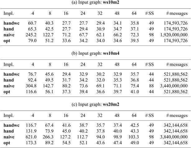
Table 3. Execution times of reAll with 4–64 worker processes on Giraph (in seconds)
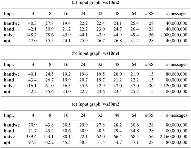
Table 4. Execution times of re100 with 4–64 worker processes on Giraph (in seconds)
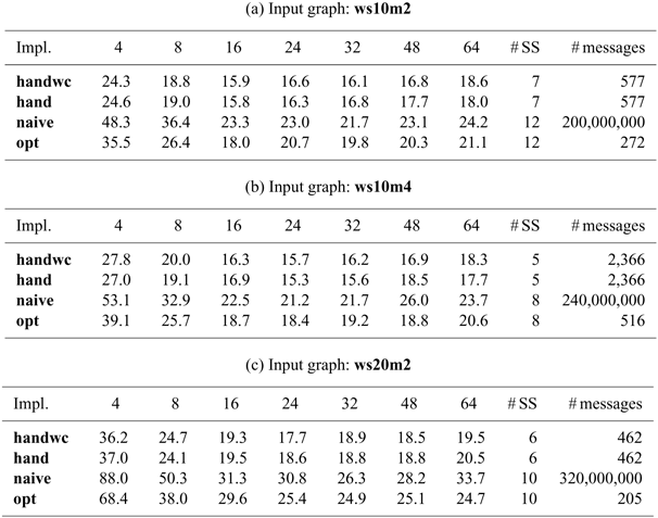
Table 5. Execution times of reRanking with 4–64 worker processes on Giraph (in seconds)
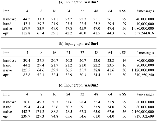
Table 6. Execution times of diameter with 4–64 worker processes on Giraph (in seconds)

Table 7. Execution times of scc with 4–64 worker processes on Giraph (in seconds)
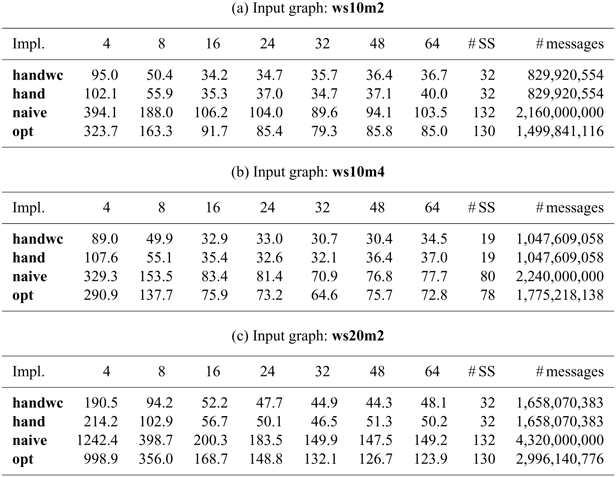
Figures 23 and 24 show the execution time of each program relative to that of handwc with 4 and 64 worker processes, respectively.he naively compiled Fregel program naive was about 4–6 times slower than handwc with 4 worker processes and about 2–3 times slower with 64 worker processes. This was due to greater numbers of messages and supersteps. The number of messages was about 2–4 times more for scc and diameter, about 10–25 times more for sssp, reAll, and reRanking, and much more for re100, which needed only a few vertices to be active. The number of supersteps was four times more for scc, which was complex enough to need many phases in the normalized program (Section 6.2), and twice as many for the other computations.he Fregel program opt (compiled with the proposed optimizations) achieved better performance than naive. The message reduction and vertex inactivation optimizations worked especially well to make the number of messages the same as that of handwc. In addition, the simple optimization to run multiple phases in a single superstep made the number of supersteps the same as that of handwc. As a result, opt was about 1.5 times slower than handwc with 4 worker processes and only 1.1 times slower with 64 worker processes. The remaining inefficiency was due to (1) opt not using combiners while handwc did and to (2) each vertex in opt having more data fields, for example, the phase number and total number of supersteps, than handwc.

Fig. 23. Computation times compared with that for handwc with four worker processes on Giraph.

Fig. 24. Computation times compared with that for handwc with 64 worker processes on Giraph.
For re100, opt used fewer messages and more supersteps than handwc. This was because handwc sent values to the aggregator and messages to its neighbors simultaneously in a single superstep to reduce the total number of supersteps, while opt performed these communications separately in two successive supersteps to reduce the number of messages.
The optimizations also worked in the more complex computations for reRanking, diameter, and scc, in which a part of the whole computation was improved by the proposed optimizations so that opt had in general fewer messages and supersteps than naive.
Figures 25–30. show the parallel performance, that is, the ratio of the actual parallel speedup to its ideal value:
 $( t_4 / t_p ) / (p / 4)$
, where
$( t_4 / t_p ) / (p / 4)$
, where
 $t_p$
is the execution time with p worker processes. First, the parallel performances of both naive and opt were not worse than that of handwc. In some cases, naive and opt achieved superlinear performance (
$t_p$
is the execution time with p worker processes. First, the parallel performances of both naive and opt were not worse than that of handwc. In some cases, naive and opt achieved superlinear performance (
 $> 1.0$
) when the number of worker processes was not large. This was because a vertex in naive and opt had more data than handwc and because there was a lack of memory when running on a small number of worker processes. In general, their performance improved as the input graph became larger.
$> 1.0$
) when the number of worker processes was not large. This was because a vertex in naive and opt had more data than handwc and because there was a lack of memory when running on a small number of worker processes. In general, their performance improved as the input graph became larger.
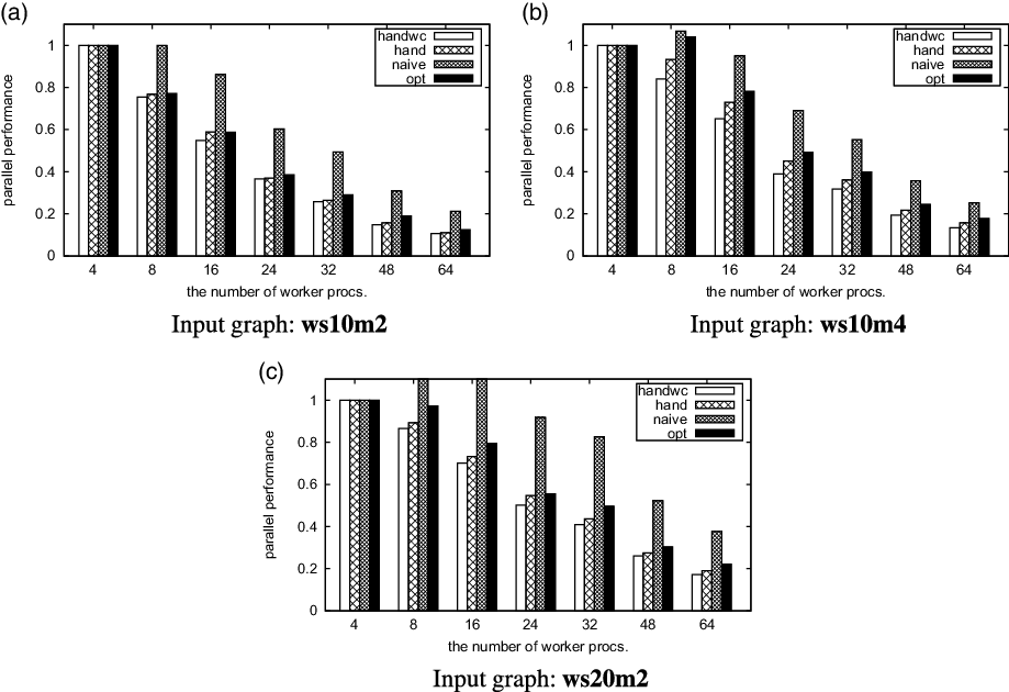
Fig. 25. Parallel performance of sssp on Giraph.
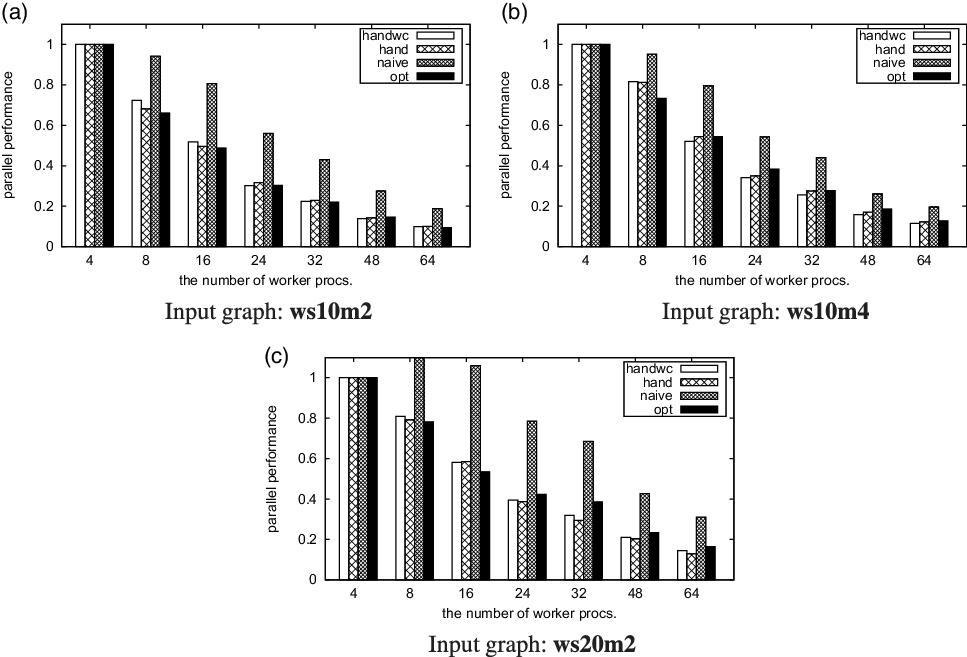
Fig. 26. Parallel performance of reAll on Giraph.
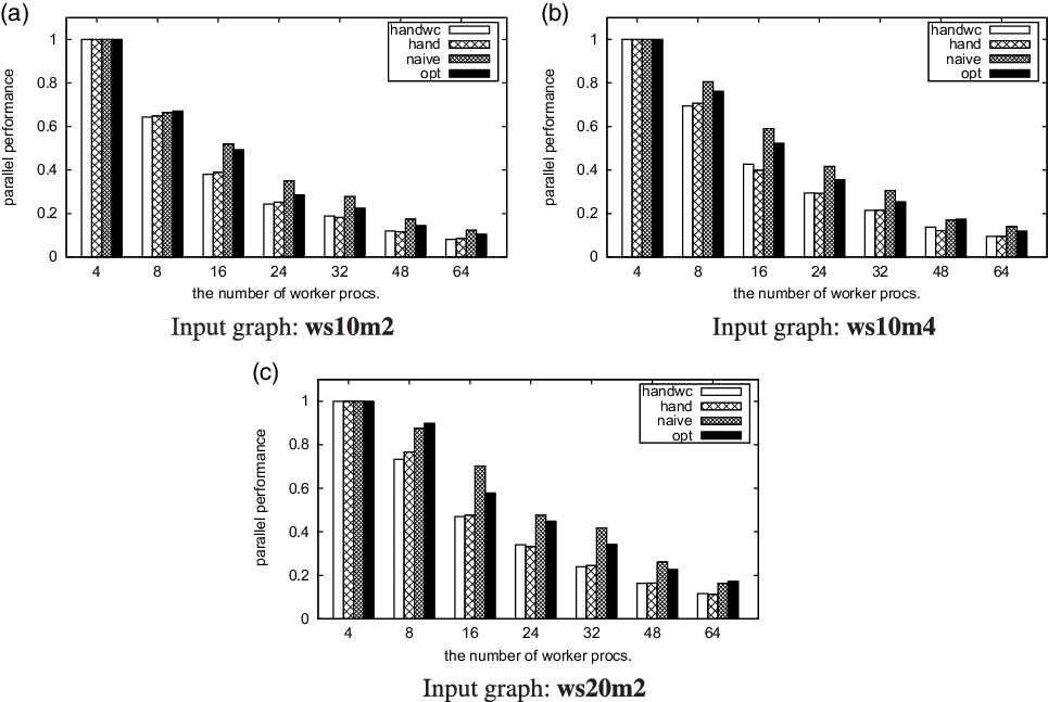
Fig. 27. Parallel performance of re100 on Giraph.
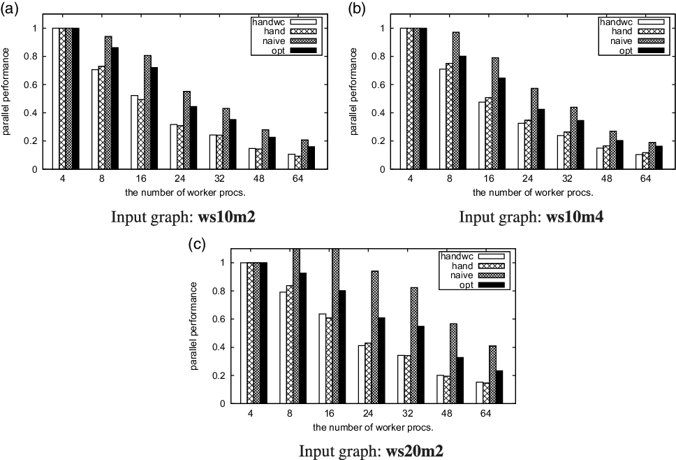
Fig. 28. Parallel performance of reRanking on Giraph.
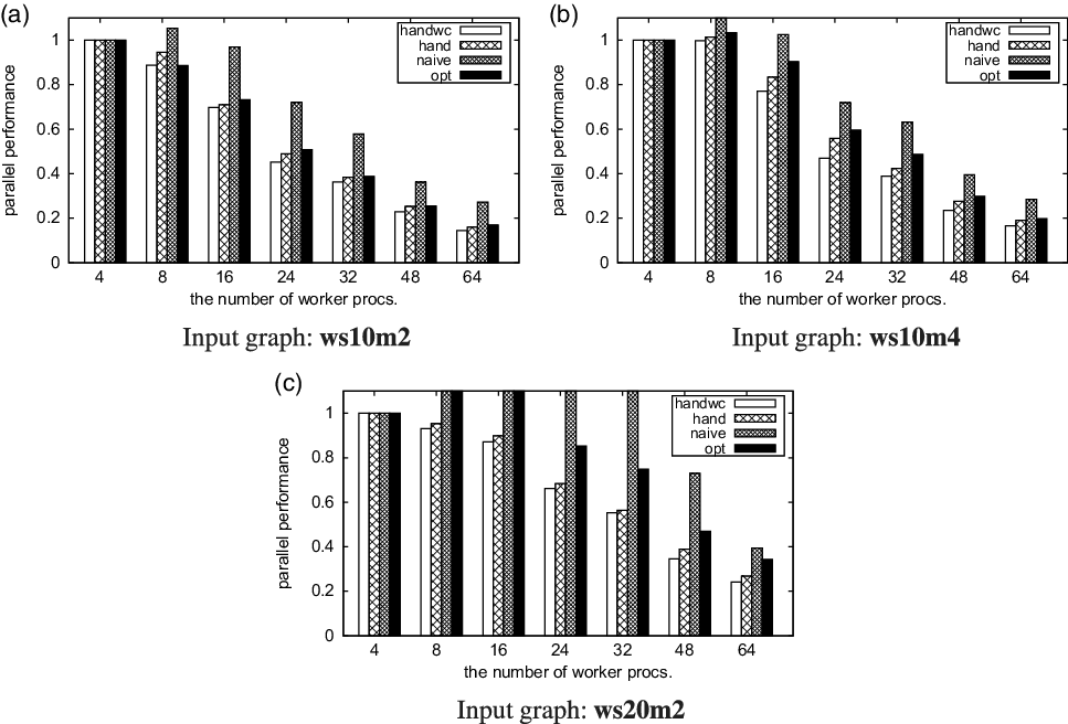
Fig. 29. Parallel performance of diameter on Giraph.
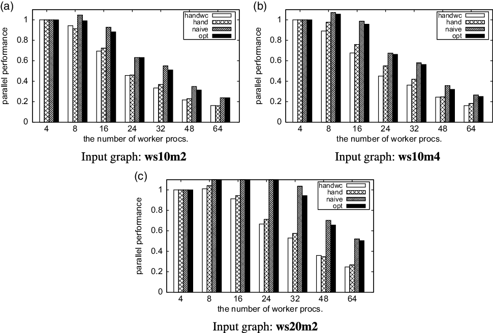
Fig. 30. Parallel performance of scc on Giraph.
To sum up, the proposed optimizations achieved reasonably good performance for both simple and complex computations.
Finally in this section, we compare memory consumption. Basically, the programs compiled from Fregel code (naive and opt) used more memory than the handwritten versions (handwc and hand). Table 8 shows the memory footprints of the vertex data fields, excluding those defined in the base class of vertices.
Table 8. Memory footprint (bytes) of vertex’s data fields in Giraph programs, excluding fields defined in the base class of vertices
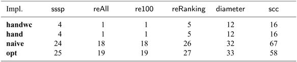
In the handwritten versions (handwc and hand), every vertex held only user-defined fields: 4 bytes for an integer for the shortest distance in sssp, 1 byte for the Boolean value for the flag in reAll, 12 bytes for three integers for the rank, the diameter, and the phase (1 or 2) in diameter, and so on. Fregel’s naively compiled program (naive) needed an additional 17–51 bytes for each vertex, which included
-
integers for the current phase, subphase, and superstep,
-
the initial value in the input graph,
-
the previous values of the user-defined fields computed in the previous phase, and
-
data used to control the phase transition (Section 6.2) caused by the use of giter , which was necessary only in scc.
For all benchmarks except scc, Fregel’s optimized program (opt) needed another byte compared with naive for the Boolean value indicating whether its user-defined fields had been changed in the superstep. For scc, the size of opt was less than that of naive because some fields were eliminated by the optimizations.
The memory consumptions for edges were the same for all benchmarks.
In summary, for a simple computation like reAll, the Fregel vertices needed much more memory than the ones in the handwritten programs due to the additional fields used for controlling the phase transition. However, this increase in the vertex memory footprint did not matter as it did not substantially increase maximum memory consumption. This is more clearly evident in the results for maximum memory consumption for Pregel+ presented in the next section. (Since Giraph uses Java, it is difficult to observe the maximum memory consumptions for Giraph.)
8.2 Compilation target: Pregel+
This section reports the experimental results for Pregel+.
Tables 9–14. show the measured execution times (the median of five runs) for the programs with 4, 8, 16, 24, 32, 48, and 64 worker processes, as well as the number of supersteps (# SS) and the number of messages (# messages). Note that the number of messages was counted after the use of combiners. Thus, the number of messages of handwc differed from that of hand.
Table 9. Execution times of sssp with 4–64 worker processes on Pregel+ (in seconds)
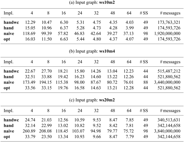
Table 10. Execution times of reAll with 4–64 worker processes on Pregel+ (in seconds)

Table 11. Execution times of re100 with 4–64 worker processes on Pregel+ (in seconds)

Table 12. Execution times of reRanking with 4–64 worker processes on Pregel+ (in seconds)
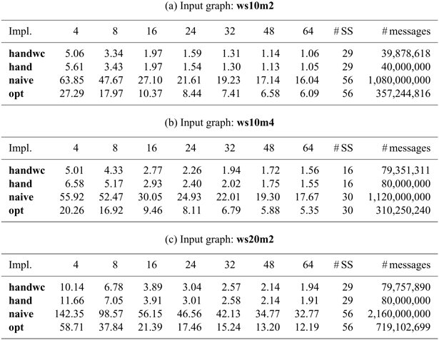
Table 13. Execution times of diameter with 4–64 worker processes on Pregel+ (in seconds)
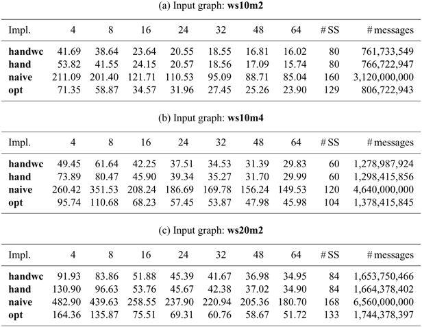
Table 14. Execution times of scc with 4–64 worker processes on Pregel+ (in seconds)

Figures 31 and 32 show the execution time of each program relative to that of handwc with 4 and 64 worker processes, respectively. Figures 33–38 show the parallel performance.
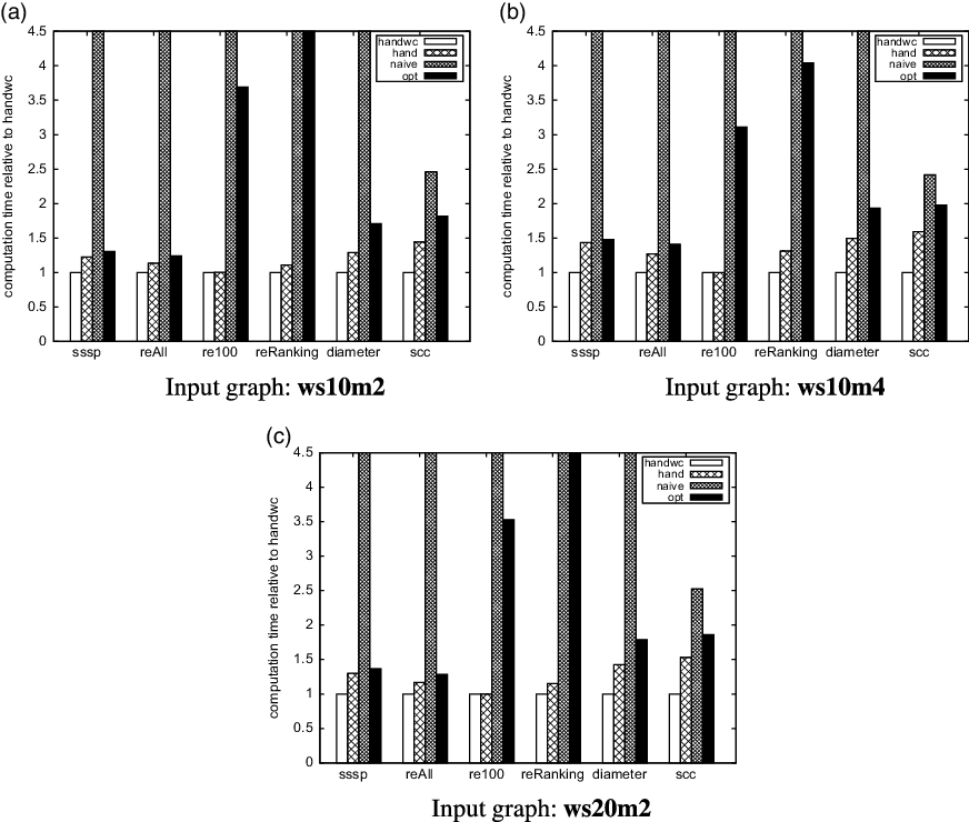
Fig. 31. Computation times compared with that for handwc with four worker processes on Pregel
 $+$
.
$+$
.

Fig. 32. Computation times compared with that for handwc with 64 worker processes on Pregel
 $+$
.
$+$
.
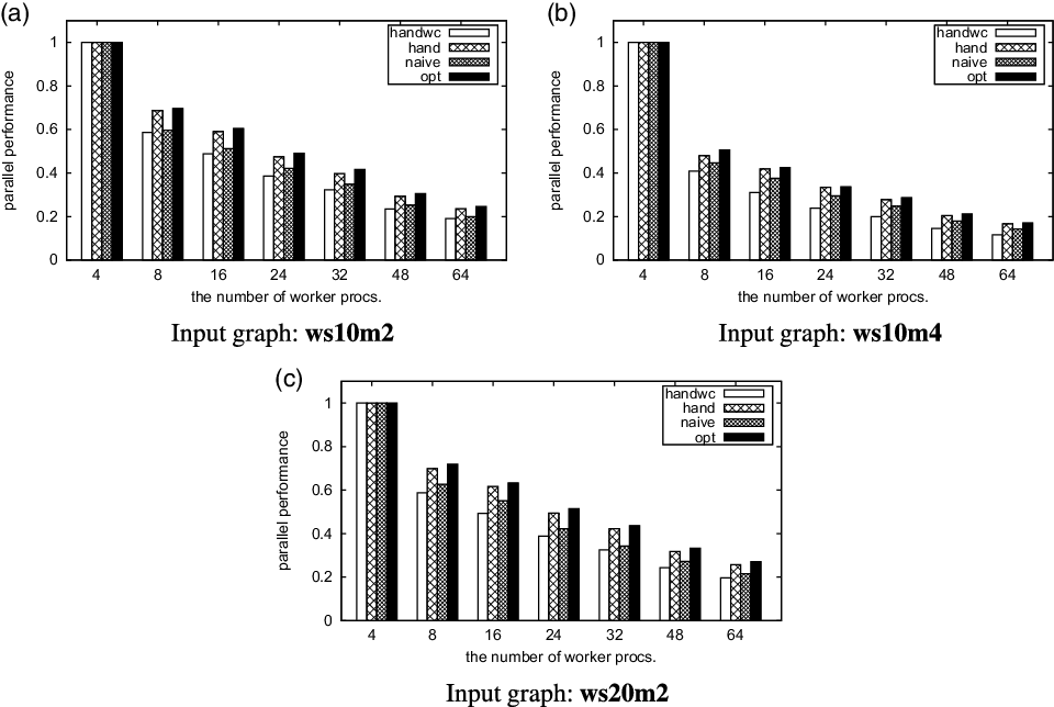
Fig. 33. Parallel performance of sssp on Pregel
 $+$
.
$+$
.
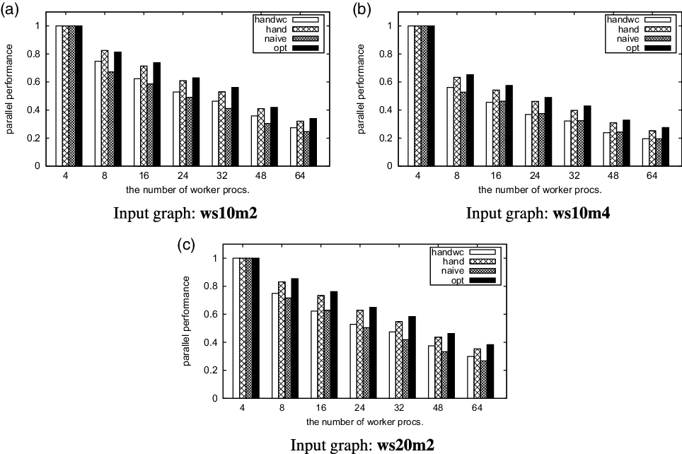
Fig. 34. Parallel performance of reAll on Pregel
 $+$
.
$+$
.

Fig. 35. Parallel performance of re100 on Pregel
 $+$
.
$+$
.

Fig. 36. Parallel performance of reRanking on Pregel
 $+$
.
$+$
.
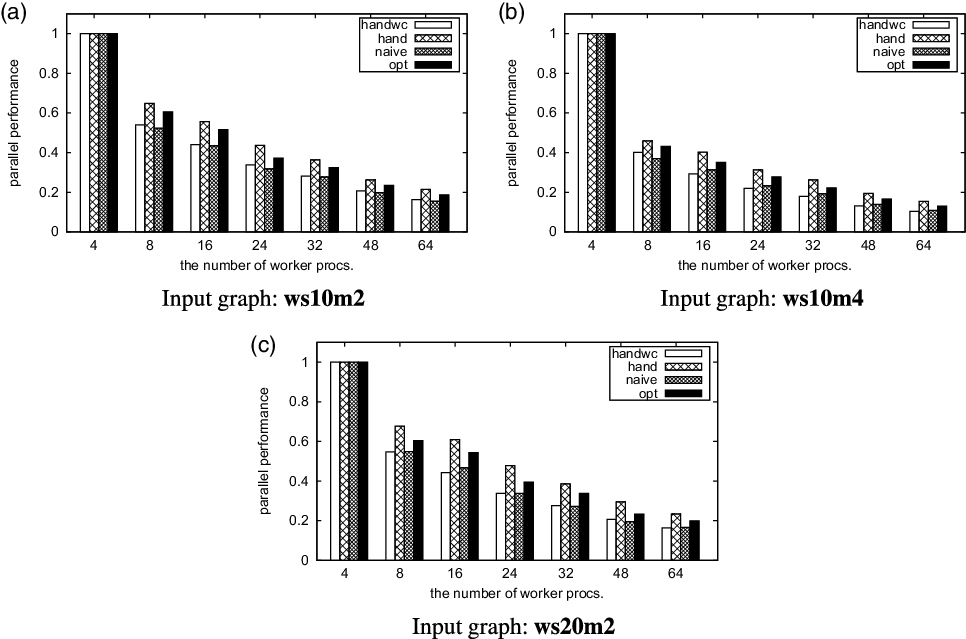
Fig. 37. arallel performance of diameter on Pregel
 $+$
.
$+$
.

Fig. 38. Parallel performance of scc on Pregel
 $+$
.
$+$
.
In general, the results show the same tendency as those for Giraph. The performance degradation of naive from handwc was much more than that for Giraph. This was because Pregel+ runs more efficiently than Giraph, so the overhead of Fregel programs was emphasized when running on Pregel+. For the same reason, no superlinear parallel performance was observed.
Table 15 shows the memory footprints of the vertex data fields, excluding those defined in the base class of vertices. The results are similar to those for Giraph (Table 8). The reason Pregel+ had a little more vertex data in many cases was that additional fields were needed for the aggregators.
Table 15. Memory footprint (bytes) of vertex data fields for Pregel+ programs, excluding fields defined in base class of vertices

Similar to the results for Giraph, memory consumption for the edges was the same for all benchmarks.
Table 16 shows the maximum memory consumption of a worker process for ws20m2. This input graph had the largest ratio of the number of vertices against that of edges among the three input graphs, and hence the effect of the vertex memory footprint on memory consumption was the largest. Each figure shows the median for five runs of the program. For each run, we took the median memory usage of all worker processes except the master process. The results show that even in the worse case (naive for re100 with four worker processes), the program compiled from Fregel code consumed only 53.1% more memory than handwc although its vertex footprint was much bigger. The increase in the amount of memory consumption decreased as the number of processes increased. These results show that the increase in the vertex memory footprint in Fregel did not cause a serious problem in terms of maximum memory consumption.
Table 16. Maximum memory consumption (MB) of a worker process for Pregel+ programs for ws20m2

In addition, for simple computations like sssp, reAll, and re100, opt consumed less memory than naive even though opt had a bigger footprint than naive. This was because opt used fewer messages and less memory space for processing messages. These results clearly show that reducing the number of messages is also effective for reducing memory consumption.
9 Related work
Vertex-centric graph processing, pioneered by Google’s Pregel (Malewicz et al. Reference Malewicz, Austern, Bik, Dehnert, Horn, Leiser and Czajkowski2010), is now a major approach to efficient large-scale graph processing. Many vertex-centric graph processing frameworks have been proposed, including Giraph, Footnote 3 GraphLab (Low et al. Reference Low, Gonzalez, Kyrola, Bickson, Guestrin and Hellerstein2012), GPS (Salihoglu & Widom Reference Salihoglu and Widom2013), GraphX (Gonzalez et al. Reference Gonzalez, Xin, Dave, Crankshaw, Franklin and Stoica2014), and Pregel+ (Yan et al. Reference Yan, Cheng, Xing, Lu, Ng and Bu2014b). Many other frameworks can be found from extensible surveys on large graph processing (Khan & Elnikety Reference Khan and Elnikety2014; McCune et al., Reference McCune, Weninger and Madey2015; Yan et al., Reference Yan, Bu, Tian, Deshpande and Cheng2016; Khan, Reference Khan2017; Yan et al., Reference Yan, Bu, Tian and Deshpande2017; Kalavri et al., Reference Kalavri, Vlassov and Haridi2018; Liu & Khan, Reference Liu and Khan2018) and experimental evaluations of these frameworks (Han et al. Reference Han, Daudjee, Ammar, Özsu, Wang and Jin2014; Lu et al., Reference Lu, Cheng, Yan and Wu2014; Guo et al., Reference Guo, Biczak, Varbanescu, Iosup, Martella and Willke2014; Satish et al., Reference Satish, Sundaram, Patwary, Seo, Park, Hassaan, Sengupta, Yin and Dubey2014; Capota et al., Reference Capota, Hegeman, Iosup, Prat-PÉrez, Erling and Boncz2015; Gao et al., Reference Gao, Zhou, Han, Meng, Zhang and Xu2015; Verma et al., Reference Verma, Leslie, Shin and Gupta2017).
Among vertex-centric graph processing frameworks, Fregel has two key features. First, its deterministic functional style makes programs concise, compositional, and easy to develop and test. Second, its optimizations eliminate major inefficiencies in naively written vertex-centric graph processing programs.
Most vertex-centric graph processing frameworks are based on sequential programming. In Section 2, we compared an existing approach with Fregel. Because of Fregel’s high-level declarative nature, programmers can write graph processing programs concisely without careful control over communications, execution states, and terminations. Second-order graph functions, fregel in particular, provide clear separation between initialization, the computation applied in each step, and the termination condition. For supporting the expressive power of Fregel as a functional vertex-centric framework, a high-level DSL (Emoto & Sadahira Reference Emoto and Sadahira2020) that is able to manipulate vertex subsets has been developed: a program written in this DSL is compiled into a Fregel program on the basis of second-order graph functions.
Several graph processing frameworks provide declarative programming interfaces, including Elixir (Prountzos et al. Reference Prountzos, Manevich and Pingali2012; Prountzos et al. Reference Prountzos, Manevich and Pingali2015), Distributed SociaLite (Seo et al. Reference Seo, Park, Shin and Lam2013), and CLM (Coordinated Linear Meld) (Cruz et al. Reference Cruz, Rocha and Goldstein2016). Elixir automatically derives an efficient distributed graph processing code from the declarative specification of the output graph. Distributed SociaLite is a graph processing language similar to Datalog. It accelerates single-source-shortest-path-like computation by processing vertices in accordance with a special priority if a certain kind of monotonicity property is detected. CLM is based on linear logic and provides control over scheduling and data layout using coordination. Interestingly, all of these frameworks are concurrent; that is, by default, the underlying graph is processed nondeterministically. In contrast, Fregel is based on BSP and therefore deterministic.
We believe that Fregel’s deterministic nature makes it easier to develop and test nontrivial graph processing programs. Moreover, Fregel’s optimizer can automatically detect possibilities of nondeterministic, that is, asynchronous, evaluation. Another difference is that existing frameworks require programmers to provide clues for optimization. For instance, with Elixir, programmers should specify the conditions for sending messages and the priorities for processing vertices. With Distributed SociaLite, prioritized execution is applied only if programmers use certain operators. CLM can generate efficient code only when programmers provide appropriate annotations called “coordination facts.”
Several recently proposed frameworks take dynamic optimization approaches. SLFE (Song et al. Reference Song, Liu, Wu, Gerstlauer, Li and John2018) reduces redundancies in vertex computation by utilizing a graph’s topological knowledge on the fly. SympleGraph (Zhuo et al. Reference Zhuo, Chen, Luo, Wang, Yang, Qian and Qian2020) eliminates unnecessary computations and communications by propagating loop-carried dependency dynamically. Unlike these frameworks, Fregel takes a static optimization approach, but the optimization methods used for Fregel are not new. Vertex inactivation is a part of the core functionality of Pregel (Malewicz et al. Reference Malewicz, Austern, Bik, Dehnert, Horn, Leiser and Czajkowski2010). The communication reduction technique for the single-source shortest path problem has been reported (Malewicz et al. Reference Malewicz, Austern, Bik, Dehnert, Horn, Leiser and Czajkowski2010). Many vertex-centric graph processing frameworks support asynchronous execution (Gonzalez et al. Reference Gonzalez, Low, Gu, Bickson and Guestrin2012; Low et al. Reference Low, Gonzalez, Kyrola, Bickson, Guestrin and Hellerstein2012; Wang et al., Reference Wang, Xie, Demers and Gehrke2013; Han & Daudjee, Reference Han and Daudjee2015); moreover, some combine asynchronous and synchronous execution to further improve efficiency (Xie et al. Reference Xie, Chen, Guan, Zang and Chen2015; Liu et al. Reference Liu, Zhou, Gao and Fan2016). Several frameworks (Prountzos et al., Reference Prountzos, Manevich and Pingali2012, Reference Prountzos, Manevich and Pingali2015; Salihoglu & Widom, Reference Salihoglu and Widom2014; Cruz et al., Reference Cruz, Rocha and Goldstein2016; Liu et al., Reference Liu, Zhou, Gao and Fan2016) support prioritized execution as well. The effectiveness of these optimizations has been intensively studied. Our contribution is their automation using constraint solvers.
Some frameworks are based on variants of vertex-centric graph processing, including subgraph-centric ones (Tian et al., Reference Tian, Balmin, Corsten, Tatikonda and McPherson2013; Simmhan et al., Reference Simmhan, Kumbhare, Wickramaarachchi, Nagarkar, Ravi, Raghavendra and Prasanna2014; Quamar et al., Reference Quamar, Deshpande and Lin2014, Reference Quamar, Deshpande and Lin2016; Quamar & Deshpande, Reference Quamar and Deshpande2016), block-centric ones (Yan et al., Reference Yan, Cheng, Lu and Ng2014a), edge-centric ones, (Zhou et al., Reference Zhou, Xu, Chen, Wang and Zhou2017), and path-centric ones (Yuan et al., Reference Yuan, Xie, Liu and Jin2016). The motivation behind these variants is that the vertex-centric approach is sometimes too fine-grained and thus potentially misses opportunities for optimization based on localities and graph structures. For example, the subgraph-centric approach processes subgraphs, rather than vertices, so a specialized algorithm can be used for determining the order and necessity of processing vertices and edges in the subgraph. To enable potential tuning of the substructures, programming with these variants tends to be more difficult than that with the vertex-centric approach because programmers need to carefully control the processing over substructures and the communications between substructures. Though Fregel is based on a vertex-centric approach, the combination of asynchronous and prioritized execution in Fregel may bring efficiency improvement similar to that obtained by using these variants. For instance, in a vertex-centric program for the single-source shortest path problem, these optimizations lead to a code that processes each subgraph by using the Dijkstra algorithm. It is not known whether our optimizations are sufficient for efficient graph processing for practical cases. Investigating this is left for future work.
Many researchers have investigated recursive approaches to programming graph algorithms in functional languages (Fegaras & Sheard, Reference Fegaras and Sheard1996; Erwig, Reference Erwig1997, Reference Erwig2001; Hamana, Reference Hamana2010; Oliveira & Cook, Reference Oliveira and Cook2012; Hidaka et al., Reference Hidaka, Asada, Hu, Kato and Nakano2013; Bahr & Axelsson, Reference Bahr and Axelsson2017). They regarded cyclic and shared structures as (possibly infinite) trees and provided a way of structural-recursive processing of the tree representations. Unfortunately, all of them are for sequential computation. Except for its focus on parallel computation, the Fregel language follows a direction similar to that of previous studies, with special attention to memorization of calculated values and termination control by observing a possibly infinite sequence of graphs.
10 Conclusion
We have presented a functional formalization of synchronous vertex-centric graph processing and proposed Fregel, a domain-specific language based on the proposed formalized model. The Fregel compiler translates a Fregel program into one that can be run in the Giraph or Pregel+ framework for parallel vertex-centric graph processing. The compiler has two key features. One is automatic division of an LSS at every communication point into Pregel supersteps to generate a normalized program, which is then transformed into a program for the target framework via framework-dependent IR. The other is automatic removal of inefficiencies, for example, unnecessary communication between vertices, by the use of a constraint solver. These features enable the Fregel programmer to develop a vertex-centric program intuitively and concisely without being concerned with how to properly control and terminate the computation on each vertex.
Our main focus has been to investigate the effects of a declarative approach to vertex-centric graph processing, for example, how the approach relieves the programmer of the complicated programming tasks when using imperative languages, for which various controls over computation have to be explicitly described. Thus, although Fregel currently has limited capabilities regarding the use of list data structures and recursive definitions, this is not a drawback because the purpose of this research is not to develop a compiler for a full-set functional language. Nevertheless, future work includes overcoming these limitations to make Fregel more practical.
Future work also includes implementing and evaluating two potential optimizations described in Sections 7.4 and 7.5. This might require developing a framework that supports both synchronous and asynchronous execution.
The latest version of the Fregel system is available via the web at https://fregel.ipl-lab.org/.
Acknowledgments
This work was partly supported by JSPS KAKENHI Grant Numbers JP26280020, JP15K15965, and JP19K11901.
Conflicts of Interest
None


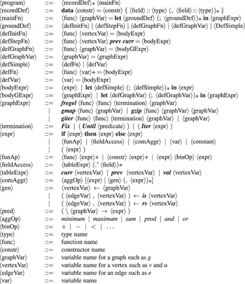


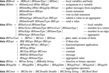


 Open access
Discussions
No Discussions have been published for this article.