


1. Introduction
Functional programmers who enjoy working with lazy data structures sometimes wish numeric computations were lazy too. Usually they are not. Even in a “lazy” functional language such as Haskell, if numeric expressions are evaluated at all, they are evaluated completely. (At least, this is true for expressions of all predefined numeric types.) Such chunks of eagerness can play havoc with the fine-grained machinery of lazy evaluation. In particular, eager numeric operations are unsuitable for delicate measurements of lazy data structures. For example, an innocent-looking comparison such as ${\textit{length}\;\textit{xs}\mathbin{>}\mathrm{0}}$
forces evaluation of the entire spine of the list
${\textit{length}\;\textit{xs}\mathbin{>}\mathrm{0}}$
forces evaluation of the entire spine of the list ${\textit{xs}}$
—a needless expense.
${\textit{xs}}$
—a needless expense.
One way to address this problem is to introduce an alternative numeric type whose values are indeed lazy data structures. Although some applications require negative or fractional values, the principal numeric requirement in general-purpose programming is support for the natural numbers (Runciman Reference Runciman1989). Following Peano (Reference Peano1889), one specific option is to declare a datatype for successor chains with zero as a terminal value.
 \begin{equation*}\mathbf{data} \, Peano=O|S \, Peano\end{equation*}
By default, S is non-strict: in accordance with an early mantra of laziness (Friedman & Wise Reference Friedman and Wise1976), successor does not evaluate its argument. So if ${\textit{length}}$
computes a successor chain,
${\textit{length}}$
computes a successor chain, ${\textit{length}\;\textit{xs}\mathbin{>}\textit{O}}$
evaluates almost immediately, as only the outermost constructor of length xs is needed to decide whether
${\textit{length}\;\textit{xs}\mathbin{>}\textit{O}}$
evaluates almost immediately, as only the outermost constructor of length xs is needed to decide whether ${\textit{O}\mathbin{>}\textit{O}\mathrel{=}\textit{False}}$
or
${\textit{O}\mathbin{>}\textit{O}\mathrel{=}\textit{False}}$
or ${\textit{S}\;\textit{n}\mathbin{>}\textit{O}\mathrel{=}\textit{True}}$
applies. This is how lazy natural numbers are implemented in the numbers library for Haskell (Augustsson Reference Augustsson2007).
${\textit{S}\;\textit{n}\mathbin{>}\textit{O}\mathrel{=}\textit{True}}$
applies. This is how lazy natural numbers are implemented in the numbers library for Haskell (Augustsson Reference Augustsson2007).
However, arithmetic succession is like a fixed small combinator—it is even called S! Performance is limited by such a fine-grained unit of work. We want a counterpart to the super-combinators of Hughes (Reference Hughes1982), attuned to the coarser-grained units of work in the computation in hand. Meet super-naturals Footnote 1 .
2. Super-naturals
Viewed another way, Peano is isomorphic to the type [()], and there are not many interesting operations on () values. A component type already equipped with arithmetic would offer more scope. So, generalising successor chains ${\mathrm{1}\mathbin{+}\mathrm{1}\mathbin{+}\cdots }$
, our lazy number structures are partitions
${\mathrm{1}\mathbin{+}\mathrm{1}\mathbin{+}\cdots }$
, our lazy number structures are partitions ${\textit{i}\mathbin{+}\textit{j}\mathbin{+}\cdots }$
where the component values
${\textit{i}\mathbin{+}\textit{j}\mathbin{+}\cdots }$
where the component values ${\textit{i}}, {\textit{j}}, \ldots$
are positive whole numbers.
${\textit{i}}, {\textit{j}}, \ldots$
are positive whole numbers.
We call these structures super-naturals. They occupy a spectrum, at the extreme ends of which are counterparts of the eager monolithic Natural Footnote 2 and the lazy fine-grained Peano. But there are many intermediate possibilities, with partitions of different sizes.

A super-natural is either zero, represented by O, or of the form ${\textit{p}\mathbin{\mathord{:}\mkern-2.5mu\mathord{+}}\textit{ps}}$
Footnote 3
where
${\textit{p}\mathbin{\mathord{:}\mkern-2.5mu\mathord{+}}\textit{ps}}$
Footnote 3
where $p$
is an evaluated part but
$p$
is an evaluated part but $ps$
may be unevaluated. The exclamation mark is a strictness annotation, forcing the first argument of
$ps$
may be unevaluated. The exclamation mark is a strictness annotation, forcing the first argument of ${\mathbin{\mathord{:}\mkern-2.5mu\mathord{+}}}$
to be fully evaluated. The first, but not the second, so
${\mathbin{\mathord{:}\mkern-2.5mu\mathord{+}}}$
to be fully evaluated. The first, but not the second, so ${\mathbin{\mathord{:}\mkern-2.5mu\mathord{+}}}$
is a form of delayed addition. The parametric natural type can, in principle, be any numeric type that implements mathematical naturals with operations for arithmetic and comparison.
${\mathbin{\mathord{:}\mkern-2.5mu\mathord{+}}}$
is a form of delayed addition. The parametric natural type can, in principle, be any numeric type that implements mathematical naturals with operations for arithmetic and comparison.
Although the invariant that all parts of a super-natural are positive is not enforced by the type system, the smart constructor ${\mathbin{\mathord{.}\mkern-2.5mu\mathord{+}}}$
takes care to avoid zero parts. An analogous smart product
${\mathbin{\mathord{.}\mkern-2.5mu\mathord{+}}}$
takes care to avoid zero parts. An analogous smart product ${\mathbin{\mathord{.}\mkern-1mu\mathord{*}}}$
will also be useful.
${\mathbin{\mathord{.}\mkern-1mu\mathord{*}}}$
will also be useful.

The type Super is parametric, even functorial in the underlying number type, as witnessed by fmap:

Indeed, super-naturals are like redecorated lists, in which ${\mathbin{\mathord{:}\mkern-2.5mu\mathord{+}}}$
as “cons” evaluates the head but not the tail, and O replaces “nil”. The functions whole and parts convert between the two views.
${\mathbin{\mathord{:}\mkern-2.5mu\mathord{+}}}$
as “cons” evaluates the head but not the tail, and O replaces “nil”. The functions whole and parts convert between the two views.

The value function reduces a super-natural to its natural value. The width and height functions locate it in the representational spectrum. The dimensional terminology reflects a diagrammatic view of super-naturals: see Figure 1 for an example.

If ${\textit{width}\;\textit{n}\leqslant \mathrm{1}}$
then n is in its most compact form, and
${\textit{width}\;\textit{n}\leqslant \mathrm{1}}$
then n is in its most compact form, and ${\textit{height}\;\textit{n}\mathrel{=}\textit{n}}$
. If
${\textit{height}\;\textit{n}\mathrel{=}\textit{n}}$
. If ${\textit{width}\;\textit{n}\mathrel{=}\textit{value}\;\textit{n}}$
then n is like a Peano chain, and
${\textit{width}\;\textit{n}\mathrel{=}\textit{value}\;\textit{n}}$
then n is like a Peano chain, and ${\textit{height}\;\textit{n}\leqslant \mathrm{1}}$
.
${\textit{height}\;\textit{n}\leqslant \mathrm{1}}$
.

Fig. 1. A diagram of the super-natural n, for which ![]() ,
, ![]() , and
, and ![]() . Unlike the Ferrers diagrams often used for partitions, we show the parts in representation order.
. Unlike the Ferrers diagrams often used for partitions, we show the parts in representation order.
3. Basic arithmetic
Let us first establish a few guiding principles we choose to adopt in our development of arithmetic and comparative operators for super-naturals.
As wide super-naturals may be derived from lazy data structures, operations on them should also be lazy, avoiding needless evaluation. However, we want to avoid the excessive widths of results that would arise if we merely replicated the unary chains of Peano arithmetic. Instead, we seek opportunities to express the arithmetic operations on super-naturals in terms of the corresponding natural operations applied to their parts. Striking a balance between the requirement for laziness, and the requirement to supply results of moderate width, we aim for arithmetic operations with results no wider than their widest argument. In particular, arithmetic on compact super-naturals (of width ${\mathrm{0}}$
or
${\mathrm{0}}$
or ${\mathrm{1}}$
) should give compact results.
${\mathrm{1}}$
) should give compact results.
As we aspire to laziness, given arguments in constructed form (O or ${\textit{p}\mathbin{\mathord{:}\mkern-2.5mu\mathord{+}}\textit{ps}}$
), we aim to produce a result in constructed form quickly. More specifically, we aim wherever possible to define super-natural operators with a bounded-demand property: only when the kth part of a result is demanded need any kth part of an argument be evaluated.
${\textit{p}\mathbin{\mathord{:}\mkern-2.5mu\mathord{+}}\textit{ps}}$
), we aim to produce a result in constructed form quickly. More specifically, we aim wherever possible to define super-natural operators with a bounded-demand property: only when the kth part of a result is demanded need any kth part of an argument be evaluated.
Another desirable characteristic of super-natural arithmetic is that operations satisfy the usual algebraic equivalences in a strong sense. Not only are the natural values of equated expressions the same (as they must be for correctness) but when evaluated they also have identical representations as super-naturals. Such strong equivalences give assurance to programmers choosing the most convenient arrangement of a compound arithmetic expression: they need not be unduly concerned about the pragmatic effect of their choice.
Addition
For the Peano representation, addition is concatenation of S-chains. For super-naturals, merely concatenating lazy partitions would miss an opportunity. We add super-naturals by zipping them together, combining their corresponding parts under natural addition, applying the middle-two interchange law ${(\textit{i}\mathbin{+}\textit{m})\mathbin{+}(\textit{j}\mathbin{+}\textit{n})\mathrel{=}(\textit{i}\mathbin{+}\textit{j})\mathbin{+}(\textit{m}\mathbin{+}\textit{n})}$
.
Footnote 4
${(\textit{i}\mathbin{+}\textit{m})\mathbin{+}(\textit{j}\mathbin{+}\textit{n})\mathrel{=}(\textit{i}\mathbin{+}\textit{j})\mathbin{+}(\textit{m}\mathbin{+}\textit{n})}$
.
Footnote 4

Viewing super-naturals as elements of a positional base 1 number system, our super-natural addition amounts to the standard school algorithm for adding multidigit numbers, but with two simplifications. (1) As the base is 1, positions do not matter, so there is no need to align digits. (2) There is no need for “carried” values as the digits can be arbitrarily large.
Instead of addition leading to wider and wider partitions, we have ${\textit{width}\;(\textit{m}\mathbin{+}\textit{n})\mathrel{=}\textit{max}\;(\textit{width}\;\textit{m})\;(\textit{width}\;\textit{n})}$
. We also have
${\textit{width}\;(\textit{m}\mathbin{+}\textit{n})\mathrel{=}\textit{max}\;(\textit{width}\;\textit{m})\;(\textit{width}\;\textit{n})}$
. We also have ${\textit{height}\;(\textit{m}\mathbin{+}\textit{n})\leqslant \textit{height}\;\textit{m}\mathbin{+}\textit{height}\;\textit{n}}$
—not an equality as the highest parts of m and n may be in different positions.
${\textit{height}\;(\textit{m}\mathbin{+}\textit{n})\leqslant \textit{height}\;\textit{m}\mathbin{+}\textit{height}\;\textit{n}}$
—not an equality as the highest parts of m and n may be in different positions.
This super-natural ${\mathbin{+}}$
is strongly commutative and associative. Because of the zip-like recursion pattern, addition also has the bounded-demand property.
${\mathbin{+}}$
is strongly commutative and associative. Because of the zip-like recursion pattern, addition also has the bounded-demand property.
Natural subtraction
It is tempting to extend the zippy approach to natural subtraction, sometimes called monus and written ${\unicode{x2238}}$
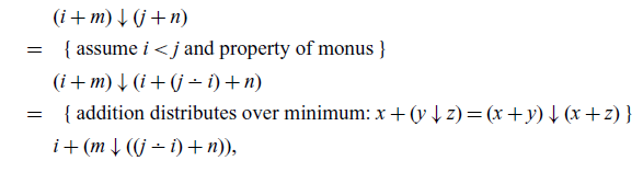
. Tempting, but wrong as the counterpart of the middle-two interchange law
${\unicode{x2238}}$
. Tempting, but wrong as the counterpart of the middle-two interchange law ${(\textit{i}\mathbin{+}\textit{m}){\unicode{x2238}}(\textit{j}\mathbin{+}\textit{n})\mathrel{=}(\textit{i}{\unicode{x2238}}\textit{j})\mathbin{+}(\textit{m}{\unicode{x2238}}\textit{n})}$
simply does not hold, e.g.
${(\textit{i}\mathbin{+}\textit{m}){\unicode{x2238}}(\textit{j}\mathbin{+}\textit{n})\mathrel{=}(\textit{i}{\unicode{x2238}}\textit{j})\mathbin{+}(\textit{m}{\unicode{x2238}}\textit{n})}$
simply does not hold, e.g. ${(\mathrm{2}\mathbin{+}\mathrm{3}){\unicode{x2238}}(\mathrm{4}\mathbin{+}\mathrm{1})\mathrel{=}\mathrm{0}\ne\mathrm{2}{=}(\mathrm{2}{\unicode{x2238}}\mathrm{4})\mathbin{+}(\mathrm{3}{\unicode{x2238}}\mathrm{1})}$
. Often, properties linking addition and subtraction are conditional as subtraction is not a full inverse of addition. Specifically,
${(\mathrm{2}\mathbin{+}\mathrm{3}){\unicode{x2238}}(\mathrm{4}\mathbin{+}\mathrm{1})\mathrel{=}\mathrm{0}\ne\mathrm{2}{=}(\mathrm{2}{\unicode{x2238}}\mathrm{4})\mathbin{+}(\mathrm{3}{\unicode{x2238}}\mathrm{1})}$
. Often, properties linking addition and subtraction are conditional as subtraction is not a full inverse of addition. Specifically, ${(\textit{a}{\unicode{x2238}}\textit{b})\mathbin{+}\textit{b}\mathrel{=}\textit{a}}$
only holds if
${(\textit{a}{\unicode{x2238}}\textit{b})\mathbin{+}\textit{b}\mathrel{=}\textit{a}}$
only holds if ${\textit{a}\geqslant \textit{b}}$
. However, there are two useful value-preserving transformations on super-naturals.
${\textit{a}\geqslant \textit{b}}$
. However, there are two useful value-preserving transformations on super-naturals.

The Oxford brackets ${[\!\![ \mbox{--}]\!\!] }$
are the semantic counterpart of value, mapping a super-natural to its denotation, an integer value—not a natural number, for reasons to become clear later.
${[\!\![ \mbox{--}]\!\!] }$
are the semantic counterpart of value, mapping a super-natural to its denotation, an integer value—not a natural number, for reasons to become clear later.
By recursive splitting, we can reduce natural subtraction of super-naturals to natural subtraction of their constituent parts. Footnote 5

Despite the possible splitting of arguments in recursive calls, the result of a super-natural subtraction has dimensions bounded by those of the first argument: ${\textit{width}\;(\textit{m}{\unicode{x2238}}\textit{n})\leqslant \textit{width}\;\textit{m}}$
and
${\textit{width}\;(\textit{m}{\unicode{x2238}}\textit{n})\leqslant \textit{width}\;\textit{m}}$
and ${\textit{height}\;(\textit{m}{\unicode{x2238}}\textit{n})\leqslant \textit{height}\;\textit{m}}$
.
${\textit{height}\;(\textit{m}{\unicode{x2238}}\textit{n})\leqslant \textit{height}\;\textit{m}}$
.
However, natural subtraction is necessarily more eager than addition. It must fully evaluate at least one argument before it can determine even the outermost construction of a result.
Of course subtraction is neither commutative nor associative. However, “subtractions commute” as we have the strong equivalence ${(\textit{k}{\unicode{x2238}}\textit{m}){\unicode{x2238}}\textit{n}\mathrel{=}(\textit{k}{\unicode{x2238}}\textit{n}){\unicode{x2238}}\textit{m}}$
. These subtraction chains are also strongly equivalent to
${(\textit{k}{\unicode{x2238}}\textit{m}){\unicode{x2238}}\textit{n}\mathrel{=}(\textit{k}{\unicode{x2238}}\textit{n}){\unicode{x2238}}\textit{m}}$
. These subtraction chains are also strongly equivalent to ${\textit{k}{\unicode{x2238}}(\textit{m}\mathbin{+}\textit{n})}$
.
${\textit{k}{\unicode{x2238}}(\textit{m}\mathbin{+}\textit{n})}$
.
Multiplication
Turning to super-natural multiplication, we need to distribute one sum over the other as illustrated in the following diagram.

One option is to enumerate the rectangles of the matrix in one way or another:
Here, ${\textit{width}\;(\textit{m}\mathbin{*}\textit{n})\mathrel{=}\textit{width}\;\textit{m}\mathbin{*}\textit{width}\;\textit{n}}$
. Such expansion is needlessly extravagant, missing opportunities for combination of natural values. To decrease the width of the resulting product, we could sum rows or columns of the matrix.
${\textit{width}\;(\textit{m}\mathbin{*}\textit{n})\mathrel{=}\textit{width}\;\textit{m}\mathbin{*}\textit{width}\;\textit{n}}$
. Such expansion is needlessly extravagant, missing opportunities for combination of natural values. To decrease the width of the resulting product, we could sum rows or columns of the matrix.

Expansion is avoided, as ${\textit{width}\;(\textit{m}\mathbin{*}\textit{n})\mathrel{=}\textit{width}\;\textit{m}}$
or
${\textit{width}\;(\textit{m}\mathbin{*}\textit{n})\mathrel{=}\textit{width}\;\textit{m}}$
or ${\mathrel{=}\textit{width}\;\textit{n}}$
. But now either
${\mathrel{=}\textit{width}\;\textit{n}}$
. But now either ${(\textit{m}\mathbin{*})}$
or
${(\textit{m}\mathbin{*})}$
or ${(\mathbin{*}\textit{n})}$
is hyper-strict—assuming natural
${(\mathbin{*}\textit{n})}$
is hyper-strict—assuming natural ${\mathbin{*}}$
is bi-strict, so natural
${\mathbin{*}}$
is bi-strict, so natural ${\textit{sum}}$
is hyper-strict. To avoid the bias toward an argument we could sum the diagonals instead (a suitable definition of diagonals is left as an exercise for the reader).
${\textit{sum}}$
is hyper-strict. To avoid the bias toward an argument we could sum the diagonals instead (a suitable definition of diagonals is left as an exercise for the reader).
Expansion is moderate as for non-O arguments: ${\textit{width}\;(\textit{m}\mathbin{*}\textit{n})\mathrel{=}\textit{width}\;\textit{m}\mathbin{+}\textit{width}\;\textit{n}\mathbin{-}\mathrm{1}}$
. However, even this expansion is questionable, and diagonalisation is quite costly.
${\textit{width}\;(\textit{m}\mathbin{*}\textit{n})\mathrel{=}\textit{width}\;\textit{m}\mathbin{+}\textit{width}\;\textit{n}\mathbin{-}\mathrm{1}}$
. However, even this expansion is questionable, and diagonalisation is quite costly.
All of these approaches are unsatisfactory in one way or another. Our preferred method of super-natural multiplication exploits the distribution of multiplication over addition in its simplest form: ${(\textit{i}\mathbin{+}\textit{m})\mathbin{*}(\textit{j}\mathbin{+}\textit{n})\mathrel{=}\textit{i}\mathbin{*}\textit{j}\mathbin{+}\textit{m}\mathbin{*}\textit{j}\mathbin{+}\textit{i}\mathbin{*}\textit{n}\mathbin{+}\textit{m}\mathbin{*}\textit{n}}$
.
${(\textit{i}\mathbin{+}\textit{m})\mathbin{*}(\textit{j}\mathbin{+}\textit{n})\mathrel{=}\textit{i}\mathbin{*}\textit{j}\mathbin{+}\textit{m}\mathbin{*}\textit{j}\mathbin{+}\textit{i}\mathbin{*}\textit{n}\mathbin{+}\textit{m}\mathbin{*}\textit{n}}$
.

Observe that three variants of multiplication are used: ${\mathbin{*}}$
is overloaded to denote both multiplication of naturals and of super-naturals,
${\mathbin{*}}$
is overloaded to denote both multiplication of naturals and of super-naturals, ${\mathbin{\mathord{.}\mkern-1mu\mathord{*}}}$
multiplies a super-natural by a natural.
${\mathbin{\mathord{.}\mkern-1mu\mathord{*}}}$
multiplies a super-natural by a natural.
Now ${\textit{width}\;(\textit{m}\mathbin{*}\textit{n})\leqslant \textit{max}\;(\textit{width}\;\textit{m})\;(\textit{width}\;\textit{n})}$
, a property acquired by the use of super-natural addition. As there is no multiplicative increase in width, there must be one in height. Indeed, the tightest bound on height in terms of argument dimensions is
${\textit{width}\;(\textit{m}\mathbin{*}\textit{n})\leqslant \textit{max}\;(\textit{width}\;\textit{m})\;(\textit{width}\;\textit{n})}$
, a property acquired by the use of super-natural addition. As there is no multiplicative increase in width, there must be one in height. Indeed, the tightest bound on height in terms of argument dimensions is
The following example is instructive. The height bound is ${\mathrm{2}\mathbin{*}\textit{min}\;\mathrm{6}\;\mathrm{6}\mathbin{*}\mathrm{1}\mathbin{*}\mathrm{1}\mathrel{=}\mathrm{12}}$
.
${\mathrm{2}\mathbin{*}\textit{min}\;\mathrm{6}\;\mathrm{6}\mathbin{*}\mathrm{1}\mathbin{*}\mathrm{1}\mathrel{=}\mathrm{12}}$
.
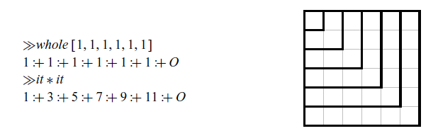
Do you recall the visual proof that the first n odd numbers sum to n squared? Well, this is exactly what is going on here. Super-natural multiplication sums up the L-shaped areas.
Multiplication defined in this way is strongly associative and commutative, and it is strongly distributive over addition. Multiplication also has the bounded-demand property.
Natural division
We defer a discussion of natural division and modulus/remainder as it will be useful to talk about comparison first.
4. Ordering
Evaluation of arithmetic expressions is typically triggered by comparisons
Footnote 6
, and the representation of super-naturals enables us to make these comparisons lazy. In particular, to decide whether a super-natural is zero, we only need to know the outermost constructor: any super-natural of the form ${\textit{p}\mathbin{\mathord{:}\mkern-2.5mu\mathord{+}}\textit{ps}}$
must be greater than zero, as all parts of a super-natural are positive. If we had negative parts, then comparison would be hyper-strict in both arguments, defeating the whole point of the exercise.
${\textit{p}\mathbin{\mathord{:}\mkern-2.5mu\mathord{+}}\textit{ps}}$
must be greater than zero, as all parts of a super-natural are positive. If we had negative parts, then comparison would be hyper-strict in both arguments, defeating the whole point of the exercise.
Comparison
The function compare employs the same recursion scheme as natural subtraction, using both comparison and subtraction over the underlying natural components.

Comparison fully evaluates the spine of one of its arguments, but rarely of both. So it exhibits similar strictness behaviour to natural subtraction, which is hardly surprising since ${\textit{a}\leqslant \textit{b}}$
if and only if
${\textit{a}\leqslant \textit{b}}$
if and only if ${\textit{a}{\unicode{x2238}}\textit{b}\mathrel{=}\mathrm{0}}$
.
${\textit{a}{\unicode{x2238}}\textit{b}\mathrel{=}\mathrm{0}}$
.
Minimum and maximum
With compare defined, Haskell defaults to generic definitions of all the boolean-valued comparison operators. These simply inspect compare results in the obvious way. There are also generic defaults for min and max
but we must not settle for these defaults. For the super-naturals they are excessively strict, giving no result until both m and n are evaluated to the extent required for compare to give its atomic result. Instead, we can give max and min their own explicit lazier definitions, re-using the recursion scheme of compare.

These definitions can be seen as productive variants of comparison. Their correctness hinges on the fact that addition distributes over both minimum ${\mathbin{\downarrow}}$
and maximum
${\mathbin{\downarrow}}$
and maximum ${\mathbin{\uparrow}}$
, e.g.:
${\mathbin{\uparrow}}$
, e.g.:
We saw that addition reduces the width of both arguments in lockstep — a zip-like pattern. By contrast, most recursive calls in the compare family of functions only reduce the width of one argument—a merge-like pattern. We see the impact in the worst-case widths of results, which for max are the sums of argument widths, and for min just one less:

The first of these examples also illustrates a curious and disappointing feature of max: it factors out the minimum of the first parts in each step, not the maximum as one might reasonably expect.
Minimum revisited
Can we rework the definition of min so that it uses a zip-like recursion pattern? Yes, we can! Consider the first recursive call in the definition of min. Instead of combining ${\textit{q}{\unicode{x2238}}\textit{p}}$
and ps to form the super-natural
${\textit{q}{\unicode{x2238}}\textit{p}}$
and ps to form the super-natural ${(\textit{q}{\unicode{x2238}}\textit{p})\mathbin{\mathord{:}\mkern-2.5mu\mathord{+}}\textit{ps}}$
we simply keep the summands apart. To this end, alongside each of the original min arguments we introduce an auxiliary “accumulator” argument.
${(\textit{q}{\unicode{x2238}}\textit{p})\mathbin{\mathord{:}\mkern-2.5mu\mathord{+}}\textit{ps}}$
we simply keep the summands apart. To this end, alongside each of the original min arguments we introduce an auxiliary “accumulator” argument.
 \begin{align*}{[\!\![ \textit{min-acc}\;\textit{m}\;\textit{ps}\;\textit{n}\;\textit{qs}]\!\!] } &{\mathrel{=}(\textit{m}\mathbin{+}[\!\![ \textit{ps}]\!\!] )\mathbin{\downarrow}(\textit{n}\mathbin{+}[\!\![ \textit{qs}]\!\!] )},\end{align*}
Correctness relies on an applicative invariant that at least one accumulator is zero. Initially, both are zero. Footnote 7

Just as we defined ${\mathbin{\mathord{.}\mkern-2.5mu\mathord{+}}}$
and
${\mathbin{\mathord{.}\mkern-2.5mu\mathord{+}}}$
and ${\mathbin{\mathord{.}\mkern-1mu\mathord{*}}}$
earlier, to combine natural and super-natural arguments, here we need an asymmetric version of minimum, called dotMin.
${\mathbin{\mathord{.}\mkern-1mu\mathord{*}}}$
earlier, to combine natural and super-natural arguments, here we need an asymmetric version of minimum, called dotMin.

Maximum revisited
Theoretically, maximum is dual to minimum. However, when we define them over super-naturals, there are fundamental obstacles in the way of a symmetric formulation. There is no convenient greatest element dual to the least element O Footnote 8 . For a non-zero super-natural, the first part gives a lower bound for the entire value, but there is no dual representation of an upper bound Footnote 9 .
So implementation of max differs in some interesting ways from min. Recall that min factors out the smaller of the first parts, e.g. reducing ${\textit{min}\;(\mathrm{9}\mathbin{\mathord{:}\mkern-2.5mu\mathord{+}}\textit{m})\;(\mathrm{2}\mathbin{\mathord{:}\mkern-2.5mu\mathord{+}}\textit{n})}$
to
${\textit{min}\;(\mathrm{9}\mathbin{\mathord{:}\mkern-2.5mu\mathord{+}}\textit{m})\;(\mathrm{2}\mathbin{\mathord{:}\mkern-2.5mu\mathord{+}}\textit{n})}$
to ${\mathrm{2}\mathbin{\mathord{:}\mkern-2.5mu\mathord{+}}\textit{min}\;((\mathrm{9}{\unicode{x2238}}\mathrm{2})\mathbin{\mathord{:}\mkern-2.5mu\mathord{+}}\textit{m})\;\textit{n}}$
. This suggests that
${\mathrm{2}\mathbin{\mathord{:}\mkern-2.5mu\mathord{+}}\textit{min}\;((\mathrm{9}{\unicode{x2238}}\mathrm{2})\mathbin{\mathord{:}\mkern-2.5mu\mathord{+}}\textit{m})\;\textit{n}}$
. This suggests that ${\textit{max}}$
should factor out the larger part, e.g. reducing the call
${\textit{max}}$
should factor out the larger part, e.g. reducing the call ${\textit{max}\;(\mathrm{9}\mathbin{\mathord{:}\mkern-2.5mu\mathord{+}}\textit{m})\;(\mathrm{2}\mathbin{\mathord{:}\mkern-2.5mu\mathord{+}}\textit{n})}$
to
${\textit{max}\;(\mathrm{9}\mathbin{\mathord{:}\mkern-2.5mu\mathord{+}}\textit{m})\;(\mathrm{2}\mathbin{\mathord{:}\mkern-2.5mu\mathord{+}}\textit{n})}$
to ${\mathrm{9}\mathbin{\mathord{:}\mkern-2.5mu\mathord{+}}\textit{max}\;\textit{m}\;((\mathrm{2}\mathbin{-}\mathrm{9})\mathbin{\mathord{:}\mkern-2.5mu\mathord{+}}\textit{n})}$
. But now the alarm bells are ringing, as
${\mathrm{9}\mathbin{\mathord{:}\mkern-2.5mu\mathord{+}}\textit{max}\;\textit{m}\;((\mathrm{2}\mathbin{-}\mathrm{9})\mathbin{\mathord{:}\mkern-2.5mu\mathord{+}}\textit{n})}$
. But now the alarm bells are ringing, as ${\mathrm{2}\mathbin{-}\mathrm{9}}$
is negative, beyond the realm of natural numbers!
${\mathrm{2}\mathbin{-}\mathrm{9}}$
is negative, beyond the realm of natural numbers!
One way out of this difficulty is to interpret the accumulators used for max “negatively”. Whereas for min-acc the argument-and-accumulator pairs represented natural sums, now, for max-acc, let these pairs represent integer differences:
 \begin{align*} {[\!\![ \textit{max-acc}\;\textit{ps}\;\textit{m}\;\textit{qs}\;\textit{n}]\!\!] } &{\mathrel{=}([\!\![ \textit{ps}]\!\!] \mathbin{-}\textit{m})\mathbin{\uparrow}([\!\![ \textit{qs}]\!\!] \mathbin{-}\textit{n})}.\end{align*}
Viewing super-naturals as base ${\mathrm{1}}$
numerals, in max-acc the m and n arguments are borrowed values, whereas in min-acc they are carried values.
${\mathrm{1}}$
numerals, in max-acc the m and n arguments are borrowed values, whereas in min-acc they are carried values.
Turning these ideas into equational definitions:

Again, correctness relies on the invariant that ${\textit{m}\mathrel{=}\mathrm{0}}$
or
${\textit{m}\mathrel{=}\mathrm{0}}$
or ${\textit{n}\mathrel{=}\mathrm{0}}$
. This invariant implies
${\textit{n}\mathrel{=}\mathrm{0}}$
. This invariant implies ${\textit{max}\;(\mathrm{0}\mathbin{-}\textit{m})\;(\textit{i}\mathbin{-}\textit{n})\mathrel{=}\textit{max}\;\mathrm{0}\;(\textit{i}\mathbin{-}\textit{n})}$
justifying the first base case, where max-acc specialises to monus! Once more we need an operator, this time
${\textit{max}\;(\mathrm{0}\mathbin{-}\textit{m})\;(\textit{i}\mathbin{-}\textit{n})\mathrel{=}\textit{max}\;\mathrm{0}\;(\textit{i}\mathbin{-}\textit{n})}$
justifying the first base case, where max-acc specialises to monus! Once more we need an operator, this time ${\mathbin{\mathord{.}\mkern-2.5mu\mathord{{\unicode{x2238}}}}}$
, to combine natural and super-natural values:
${\mathbin{\mathord{.}\mkern-2.5mu\mathord{{\unicode{x2238}}}}}$
, to combine natural and super-natural values:

Look again at the last equation of max-acc. As its argument–accumulator pairs represent integer differences, we factor out the maximum of ${\textit{p}\mathbin{-}\textit{m}}$
and
${\textit{p}\mathbin{-}\textit{m}}$
and ${\textit{q}\mathbin{-}\textit{n}}$
to form the first part. However, this maximum difference is sure to be positive—recall the applicative invariant for max-acc, and the data invariant that super-natural parts are positive. So replacing any negative difference by zero does not alter max’s choice: it returns the other (positive) difference. Writing
${\textit{q}\mathbin{-}\textit{n}}$
to form the first part. However, this maximum difference is sure to be positive—recall the applicative invariant for max-acc, and the data invariant that super-natural parts are positive. So replacing any negative difference by zero does not alter max’s choice: it returns the other (positive) difference. Writing ${\textit{max}\;(\textit{p}{\unicode{x2238}}\textit{m})\;(\textit{q}{\unicode{x2238}}\textit{n})}$
for
${\textit{max}\;(\textit{p}{\unicode{x2238}}\textit{m})\;(\textit{q}{\unicode{x2238}}\textit{n})}$
for ${(\textit{p}\mathbin{-}\textit{m})\mathbin{\uparrow}(\textit{q}\mathbin{-}\textit{n})}$
is not only valid, it avoids undefined results when standard subtraction is partially defined for natural.
${(\textit{p}\mathbin{-}\textit{m})\mathbin{\uparrow}(\textit{q}\mathbin{-}\textit{n})}$
is not only valid, it avoids undefined results when standard subtraction is partially defined for natural.
As the definition of max-acc is probably the most complicated in the paper, we provide a derivation in Appendix 2.
Properties revisited
So have we curtailed the sum-of-widths behaviour of max and min? Yes, as desired, we now have ${\textit{width}\;(\textit{newmax}\;\textit{m}\;\textit{n})\leqslant \textit{max}\;(\textit{width}\;\textit{m})\;(\textit{width}\;\textit{n})}$
and
${\textit{width}\;(\textit{newmax}\;\textit{m}\;\textit{n})\leqslant \textit{max}\;(\textit{width}\;\textit{m})\;(\textit{width}\;\textit{n})}$
and ${\textit{width}\;(\textit{newmin}\;\textit{m}\;\textit{n})\leqslant \textit{max}\;(\textit{width}\;\textit{m})\;(\textit{width}\;\textit{n})}$
. With min on the left, one might expect min on the right, but that inequality does not hold: e.g.
${\textit{width}\;(\textit{newmin}\;\textit{m}\;\textit{n})\leqslant \textit{max}\;(\textit{width}\;\textit{m})\;(\textit{width}\;\textit{n})}$
. With min on the left, one might expect min on the right, but that inequality does not hold: e.g. ${\textit{newmin}\;(\mathrm{1}\mathbin{\mathord{:}\mkern-2.5mu\mathord{+}}\mathrm{1}\mathbin{\mathord{:}\mkern-2.5mu\mathord{+}}\textit{O})\;(\mathrm{2}\mathbin{\mathord{:}\mkern-2.5mu\mathord{+}}\textit{O})\mathrel{=}\mathrm{1}\mathbin{\mathord{:}\mkern-2.5mu\mathord{+}}\mathrm{1}\mathbin{\mathord{:}\mkern-2.5mu\mathord{+}}\textit{O}}$
. We also have corresponding bounds on height as
${\textit{newmin}\;(\mathrm{1}\mathbin{\mathord{:}\mkern-2.5mu\mathord{+}}\mathrm{1}\mathbin{\mathord{:}\mkern-2.5mu\mathord{+}}\textit{O})\;(\mathrm{2}\mathbin{\mathord{:}\mkern-2.5mu\mathord{+}}\textit{O})\mathrel{=}\mathrm{1}\mathbin{\mathord{:}\mkern-2.5mu\mathord{+}}\mathrm{1}\mathbin{\mathord{:}\mkern-2.5mu\mathord{+}}\textit{O}}$
. We also have corresponding bounds on height as ${\textit{height}\;(\textit{newmax}\;\textit{m}\;\textit{n})\leqslant \textit{max}\;(\textit{height}\;\textit{m})\;(\textit{height}\;\textit{n})}$
and
${\textit{height}\;(\textit{newmax}\;\textit{m}\;\textit{n})\leqslant \textit{max}\;(\textit{height}\;\textit{m})\;(\textit{height}\;\textit{n})}$
and ${\textit{height}\;(\textit{newmin}\;\textit{m}\;\textit{n})\leqslant \textit{max}\;(\textit{height}\;\textit{m})\;(\textit{height}\;\textit{n})}$
. Here again, for
${\textit{height}\;(\textit{newmin}\;\textit{m}\;\textit{n})\leqslant \textit{max}\;(\textit{height}\;\textit{m})\;(\textit{height}\;\textit{n})}$
. Here again, for ${\textit{newmin}}$
a minimum depth variant is plausible but wrong: e.g.
${\textit{newmin}}$
a minimum depth variant is plausible but wrong: e.g. ${\textit{newmin}\;(\mathrm{1}\mathbin{\mathord{:}\mkern-2.5mu\mathord{+}}\mathrm{3}\mathbin{\mathord{:}\mkern-2.5mu\mathord{+}}\textit{O})\;(\mathrm{2}\mathbin{\mathord{:}\mkern-2.5mu\mathord{+}}\mathrm{2}\mathbin{\mathord{:}\mkern-2.5mu\mathord{+}}\textit{O})\mathrel{=}\mathrm{1}\mathbin{\mathord{:}\mkern-2.5mu\mathord{+}}\mathrm{3}\mathbin{\mathord{:}\mkern-2.5mu\mathord{+}}\textit{O}}$
.
${\textit{newmin}\;(\mathrm{1}\mathbin{\mathord{:}\mkern-2.5mu\mathord{+}}\mathrm{3}\mathbin{\mathord{:}\mkern-2.5mu\mathord{+}}\textit{O})\;(\mathrm{2}\mathbin{\mathord{:}\mkern-2.5mu\mathord{+}}\mathrm{2}\mathbin{\mathord{:}\mkern-2.5mu\mathord{+}}\textit{O})\mathrel{=}\mathrm{1}\mathbin{\mathord{:}\mkern-2.5mu\mathord{+}}\mathrm{3}\mathbin{\mathord{:}\mkern-2.5mu\mathord{+}}\textit{O}}$
.
As for equivalences, newmin is strongly commutative, associative and idempotent. However, newmax only scores two out of three, as it is not strongly associative. Here is a counter-example:

As for laziness, newmin has the bounded-demand property, but newmax does not share this property. Here is a counter-example:
To determine the second part (if any) of the result, newmax needs to evaluate beyond the second part of the second argument. Does the first part of the result already hold the entire maximum value, or will the second argument eventually exceed it?
We deliberately made the first part of a non-zero newmax result the natural maximum of the first parts of its arguments. This choice is consistent with laziness: it derives as much information as possible from immediately available argument parts, reducing the likelihood that any further result part (and therefore further argument parts) will be needed. Putting the previous example in a larger context:

The result would have been ${\bot }$
using our original super-natural max. However, in other contexts, where more parts of a newmax result are needed and an initially maximal argument is exhausted, the other argument may have to be evaluated beyond the limits for a bounded-demand operation. We cannot have our cake and eat it!
${\bot }$
using our original super-natural max. However, in other contexts, where more parts of a newmax result are needed and an initially maximal argument is exhausted, the other argument may have to be evaluated beyond the limits for a bounded-demand operation. We cannot have our cake and eat it!
5. Super-natural division
Super-natural division with remainder is a more tricky problem. Resorting to repeated subtraction would be no more attractive than mere repeated addition was for multiplication. Instead we seek a way to apply natural division to component parts.
As a warm-up, let us first complete our family of point-wise operations: ${\textit{dotDiv}}$
is a special case of natural division where the divisor is a natural, rather than a super-natural.
${\textit{dotDiv}}$
is a special case of natural division where the divisor is a natural, rather than a super-natural.

The recursive case is derived by join and split transformations: the super-natural dividend ${\textit{p}_{1}\mathbin{\mathord{:}\mkern-2.5mu\mathord{+}}\textit{p}_{2}\mathbin{\mathord{:}\mkern-2.5mu\mathord{+}}\textit{ps}}$
, which equals
${\textit{p}_{1}\mathbin{\mathord{:}\mkern-2.5mu\mathord{+}}\textit{p}_{2}\mathbin{\mathord{:}\mkern-2.5mu\mathord{+}}\textit{ps}}$
, which equals ${((\textit{p}_{1}\mathbin{\textbf{div}}\textit{d})\mathbin{*}\textit{d}\mathbin{+}\textit{p}_{1}\mathbin{\textbf{mod}}\textit{d})\mathbin{\mathord{:}\mkern-2.5mu\mathord{+}}\textit{p}_{2}\mathbin{\mathord{:}\mkern-2.5mu\mathord{+}}\textit{ps}}$
, is rewritten to the super-natural
${((\textit{p}_{1}\mathbin{\textbf{div}}\textit{d})\mathbin{*}\textit{d}\mathbin{+}\textit{p}_{1}\mathbin{\textbf{mod}}\textit{d})\mathbin{\mathord{:}\mkern-2.5mu\mathord{+}}\textit{p}_{2}\mathbin{\mathord{:}\mkern-2.5mu\mathord{+}}\textit{ps}}$
, is rewritten to the super-natural ${(\textit{p}_{1}\mathbin{\textbf{div}}\textit{d})\mathbin{*}\textit{d}\mathbin{\mathord{:}\mkern-2.5mu\mathord{+}}(\textit{p}_{1}\mathbin{\textbf{mod}}\textit{d}\mathbin{+}\textit{p}_{2})\mathbin{\mathord{:}\mkern-2.5mu\mathord{+}}\textit{ps}}$
.
${(\textit{p}_{1}\mathbin{\textbf{div}}\textit{d})\mathbin{*}\textit{d}\mathbin{\mathord{:}\mkern-2.5mu\mathord{+}}(\textit{p}_{1}\mathbin{\textbf{mod}}\textit{d}\mathbin{+}\textit{p}_{2})\mathbin{\mathord{:}\mkern-2.5mu\mathord{+}}\textit{ps}}$
.
Concerning division of super-naturals, ${\textit{a}\mathbin{\textbf{div}}\textit{b}}$
cannot be lazier than
${\textit{a}\mathbin{\textbf{div}}\textit{b}}$
cannot be lazier than ${\textit{a}\mathbin{<}\textit{b}}$
because we can implement
${\textit{a}\mathbin{<}\textit{b}}$
because we can implement ${\mathbin{<}}$
in terms of
${\mathbin{<}}$
in terms of ${\mathbin{\textbf{div}}}: {\textit{a}\mathbin{<}\textit{b}}$
if and only if
${\mathbin{\textbf{div}}}: {\textit{a}\mathbin{<}\textit{b}}$
if and only if ${\textit{a}\mathbin{\textbf{div}}\textit{b}\mathrel{=}\mathrm{0}}$
. To compute
${\textit{a}\mathbin{\textbf{div}}\textit{b}\mathrel{=}\mathrm{0}}$
. To compute ${\textit{a}\mathbin{\textbf{mod}}\textit{b}}$
, complete evaluation of a is required; indeed, there is no sensible, lazy dotMod operation.
${\textit{a}\mathbin{\textbf{mod}}\textit{b}}$
, complete evaluation of a is required; indeed, there is no sensible, lazy dotMod operation.

This definition squeezes out the last bit of laziness: if ${\textit{a}\mathbin{<}\textit{b}}$
then
${\textit{a}\mathbin{<}\textit{b}}$
then ${\textit{a}\mathbin{\textbf{mod}}\textit{b}\mathrel{=}\textit{a}}$
; we can return a in compact form as it is fully evaluated by the comparison, but b need not be fully evaluated. However, if
${\textit{a}\mathbin{\textbf{mod}}\textit{b}\mathrel{=}\textit{a}}$
; we can return a in compact form as it is fully evaluated by the comparison, but b need not be fully evaluated. However, if ${\textit{a}\mathbin{>}\textit{b}}$
then
${\textit{a}\mathbin{>}\textit{b}}$
then ${\textit{a}\mathbin{\textbf{mod}}\textit{b}}$
is inevitably eager.
${\textit{a}\mathbin{\textbf{mod}}\textit{b}}$
is inevitably eager.
Like subtraction, division gives results with dimensions bounded by those of the first argument, despite possible additions to its parts in recursive calls. That is, assuming non-O n, we have both ${\textit{width}\;(\textit{m}\mathbin{\textbf{div}}\textit{n})\leqslant \textit{width}\;\textit{m}}$
and
${\textit{width}\;(\textit{m}\mathbin{\textbf{div}}\textit{n})\leqslant \textit{width}\;\textit{m}}$
and ${\textit{height}\;(\textit{m}\mathbin{\textbf{div}}\textit{n})\leqslant \textit{height}\;\textit{m}}$
. All remainders are compact:
${\textit{height}\;(\textit{m}\mathbin{\textbf{div}}\textit{n})\leqslant \textit{height}\;\textit{m}}$
. All remainders are compact: ${\textit{width}\;(\textit{m}\mathbin{\textbf{mod}}\textit{n})\leqslant \mathrm{1}}$
and
${\textit{width}\;(\textit{m}\mathbin{\textbf{mod}}\textit{n})\leqslant \mathrm{1}}$
and ${\textit{height}\;(\textit{m}\mathbin{\textbf{mod}}\textit{n})\mathbin{<}\textit{value}\;\textit{n}}$
.
${\textit{height}\;(\textit{m}\mathbin{\textbf{mod}}\textit{n})\mathbin{<}\textit{value}\;\textit{n}}$
.
Also like subtraction, division is neither commutative nor associative, yet “divisions commute” as the strong equivalence ${(\textit{k}\mathbin{\textbf{div}}\textit{m})\mathbin{\textbf{div}}\textit{n}\mathrel{=}(\textit{k}\mathbin{\textbf{div}}\textit{n})\mathbin{\textbf{div}}\textit{m}}$
holds. These division chains are also strongly equivalent to
${(\textit{k}\mathbin{\textbf{div}}\textit{m})\mathbin{\textbf{div}}\textit{n}\mathrel{=}(\textit{k}\mathbin{\textbf{div}}\textit{n})\mathbin{\textbf{div}}\textit{m}}$
holds. These division chains are also strongly equivalent to ${\textit{k}\mathbin{\textbf{div}}(\textit{m}\mathbin{*}\textit{n})}$
. Any equivalence between
${\textit{k}\mathbin{\textbf{div}}(\textit{m}\mathbin{*}\textit{n})}$
. Any equivalence between ${\mathbin{\textbf{mod}}}$
results is guaranteed to be a strong equivalence, as all such results are compact.
${\mathbin{\textbf{mod}}}$
results is guaranteed to be a strong equivalence, as all such results are compact.
6. Application: measures
Returning to our introductory motivation, in this section we explore the use of super-natural arithmetic to measure lazy data structures.
Measuring binary search trees
There are at least three different measures of a binary search tree: the number of keys stored in it (size), the length of the shortest path from the root to a leaf (min-height), and the length of the longest one (max-height).

These definitions may look quite standard, but there is an important twist: in some places they use delayed addition ${\mathbin{\mathord{:}\mkern-2.5mu\mathord{+}}}$
rather than overloaded addition
${\mathbin{\mathord{:}\mkern-2.5mu\mathord{+}}}$
rather than overloaded addition ${\mathbin{+}}$
. Why? Because if these functions used only the methods of the predefined numeric classes, they would exhibit the very strict behaviour we deprecated in our introduction.
${\mathbin{+}}$
. Why? Because if these functions used only the methods of the predefined numeric classes, they would exhibit the very strict behaviour we deprecated in our introduction.
The size function uses both delayed and overloaded addition, which has an interesting effect. To showcase its behaviour, we first define an insert function as a way to grow trees.

Now we generate a list of a million random elements, fold this list by insertion into a large search tree, and measure it.

By the combined application of ${\mathbin{\mathord{:}\mkern-2.5mu\mathord{+}}}$
and
${\mathbin{\mathord{:}\mkern-2.5mu\mathord{+}}}$
and ${\mathbin{+}}, {\textit{size}}$
processes the tree breadth-first, and the k-th part of its result is the number of elements on level k! The first
${\mathbin{+}}, {\textit{size}}$
processes the tree breadth-first, and the k-th part of its result is the number of elements on level k! The first ${\mathrm{7}}$
parts are exact powers of two, which tells us that the first
${\mathrm{7}}$
parts are exact powers of two, which tells us that the first ${\mathrm{7}}$
levels of the tree are full. But then the leaves start, so the tree’s minimal height is
${\mathrm{7}}$
levels of the tree are full. But then the leaves start, so the tree’s minimal height is ${\mathrm{7}}$
. Finally, the width of this super-natural size gives us the maximal height of the tree—it is
${\mathrm{7}}$
. Finally, the width of this super-natural size gives us the maximal height of the tree—it is ${\mathrm{48}}$
.
${\mathrm{48}}$
.
The two functions measuring path lengths behave quite differently. Thanks to lazy evaluation, min-height is a lot faster than max-height—around $3\times$
faster, for this example.
$3\times$
faster, for this example.

These measure functions also work smoothly with infinite trees. To illustrate, grow-except grows an infinite tree with only a single leaf at some given position.

Any result of grow-except has infinite size and infinite maximal height, but because of the leaf it has finite minimal height.

As expected, computations requiring only a finite prefix of infinite max-height or size results do not diverge. The last call, for example, returns almost instantly.
However, these example evaluations also demonstrate that the height functions return only successor chains. Such chains may be tolerable for height measures of “bushy” structures such as trees. But what about structures with a unit branching factor, such as the ubiquitous list?
Measuring lists
For lists, the three measure functions size, min-height and max-height coincide: all are equivalent to length. So first, let us similarly define a variant of Haskell’s length function that gives a super-natural result, just replacing the single ${\mathbin{+}}$
in the usual definition by
${\mathbin{+}}$
in the usual definition by ${\mathbin{\mathord{:}\mkern-2.5mu\mathord{+}}}$
.
${\mathbin{\mathord{:}\mkern-2.5mu\mathord{+}}}$
.

The length of a list is now given by an equally long successor chain. Even though super-natural arithmetic is quite well-behaved—we have been careful to ensure that the results of arithmetic operations are no wider than their widest argument—by pursuing the goal of laziness, we seem to have boxed ourselves into a corner with Peano!
How can we compute narrower and higher super-natural lengths, without abandoning laziness and reverting to compact atomic values? Recall our width-limiting approach to arithmetic. Given two super-naturals to be added, for example, we zipped them together, typically obtaining a higher result. Though we only have a single super-natural length, we can zip it with itself by lazily splitting its parts into two super-natural “halves” and adding them together. Instead of fiddling with the length definition, we prefer a modular approach. We introduce a general-purpose combinator for super-natural compression.

Now there is a simple and modular way to obtain more compact super-natural lengths: apply ${\textit{compress}{\;.\;}\textit{length}}$
. If even compressed super-natural lengths are still too wide, here is one of many ways to achieve greater compaction: the progressively tighter squeeze function halves width again for each successive part.
${\textit{compress}{\;.\;}\textit{length}}$
. If even compressed super-natural lengths are still too wide, here is one of many ways to achieve greater compaction: the progressively tighter squeeze function halves width again for each successive part.

For example, squeezing an infinite successor chain yields the powers of two.

There is not much difference in running time between ${\textit{squeeze}\;(\textit{whole}\;[\mskip1.5mu \mathrm{1}\mathinner{\ldotp\ldotp}\mskip1.5mu])\mathbin{>}\mathrm{1000000}}$
and
${\textit{squeeze}\;(\textit{whole}\;[\mskip1.5mu \mathrm{1}\mathinner{\ldotp\ldotp}\mskip1.5mu])\mathbin{>}\mathrm{1000000}}$
and ${\textit{whole}\;[\mskip1.5mu \mathrm{1}\mathinner{\ldotp\ldotp}\mskip1.5mu]\mathbin{>}\mathrm{1000000}}$
. But the squeezed version consumes less memory.
${\textit{whole}\;[\mskip1.5mu \mathrm{1}\mathinner{\ldotp\ldotp}\mskip1.5mu]\mathbin{>}\mathrm{1000000}}$
. But the squeezed version consumes less memory.
7. Summary and concluding remarks
There is quite a gulf between atomic numeric values and Peano chains. We set out to span this gulf by developing numeric operations for a flexible intermediate representation—the super-natural number. Allowing many alternative representations for the same value gives programmers flexibility. They can choose, in any specific application, what degree of strictness or laziness they prefer. In practice, their overall choice is most simply expressed as a particular combination of individual choices between delayed and zipped super-natural addition. Even the two extreme options of atomic values (always zip, stay compact) and Peano chains (always delay, stay unary) are still available.
Non-zero super-naturals are simply partitions, freely ordered in any convenient sequence, and typically evaluated in that order. We never seriously considered any stronger data invariant. We did briefly consider a weaker one, allowing zero parts, but rejected it as it seemed to cause more problems than it solved.
In our development of the other numeric operations, we aimed to be even handed. They had to be lazy, but not so lazy as to expand super-natural widths beyond those of the widest operands. We tried hard to define operations to satisfy all the equivalences a programmer might reasonably expect. We checked all the properties we claim by testing the first million cases, and some by constructing a general proof. Addition, multiplication and minimum are particularly well-behaved; subtraction, division and remainder are of necessity stricter and asymmetric, yet still satisfy some pleasing laws; maximum is the worst-behaved—if any reader thinks they know how to reform it, please tell us!
Thinking of the relationship between numbers and lazy data structures, various data structures have been modelled after number systems. We have already observed in more than one context that the structure of lists matches the Peano number type. The textbook by Okasaki (Reference Okasaki1998) contains a wealth of further examples. In due time, perhaps someone will devise a general-purpose data structure modelled after super-naturals.
Meanwhile, super-naturals themselves are already data structures. They are containers of part values of their parametric natural type. They even meet their own requirements for such parts. Super-super-naturals anyone?
Acknowledgements
We thank Jeremy Gibbons, John Hughes and three anonymous reviewers for their helpful comments on a previous version of this article.
Conflicts of interest
None.
1. Appendix: Class instances
Haskell predefines an elaborate hierarchy of numeric type classes: Num, Real, Integral, Fractional, Floating, RealFrac, and RealFloat. Unfortunately, even the base class Num includes negation, absolute value, and sign. So natural number types do not enjoy natural instance definitions. For example, the predefined type of natural numbers (in Numeric.Natural) has a partial subtraction operation: applications such as ${\mathrm{11}\mathbin{-}\mathrm{47}}$
raise an arithmetic underflow exception.
${\mathrm{11}\mathbin{-}\mathrm{47}}$
raise an arithmetic underflow exception.
To avoid assumptions about subtraction in the underlying natural arithmetic, for the super-naturals, we introduce a custom type class for natural subtraction.

The default definition of monus uses explicit case distinction, rather than ${\textit{max}\;\mathrm{0}\;(\textit{a}\mathbin{-}\textit{b})}$
, as max is typically bi-strict.
${\textit{max}\;\mathrm{0}\;(\textit{a}\mathbin{-}\textit{b})}$
, as max is typically bi-strict.

Figures 2, 3, 4, and 5 give the instance declarations for non-numeric type classes (Functor and Show), basic arithmetic (Num), equality and comparison (Eq and Ord), and enumeration and integral operations (Enum, Real, and Integral). Each numeric type-class instance requires that the underlying natural parts type is an instance of Monus.

Fig. 2. Super-naturals: non-numeric instances.

Fig. 3. Super-naturals: basic arithmetic.

Fig. 4. Super-naturals: equality and comparison.

Fig. 5. Super-naturals: enumeration and integral operations.
2. Appendix: Derivation of max-acc
The Oxford brackets map a partition to its denotation, an integer value.
 \begin{align}{[\!\![ \textit{O}]\!\!] } &{\mathrel{=}\mathrm{0}} \end{align}
 \begin{align}{[\!\![ \textit{p}\mathbin{\mathord{:}\mkern-2.5mu\mathord{+}}\textit{ps}]\!\!] } &{\mathrel{=}\textit{p}\mathbin{+}[\!\![ \textit{ps}]\!\!] }\end{align}
Recall that the argument-and-accumulator pairs of max-acc represent integer differences:
 \begin{align}{[\!\![ \textit{max-acc}\;\textit{ps}\;\textit{m}\;\textit{qs}\;\textit{n}]\!\!] } &{\mathrel{=}([\!\![ \textit{ps}]\!\!] \mathbin{-}\textit{m})\mathbin{\uparrow}([\!\![ \textit{qs}]\!\!] \mathbin{-}\textit{n})}.\end{align}
The derivation of max-acc relies furthermore on the applicative invariant that at least one accumulator is zero: ${\textit{m}\mathrel{=}\mathrm{0}}$
or
${\textit{m}\mathrel{=}\mathrm{0}}$
or ${\textit{n}\mathrel{=}\mathrm{0}}$
.
${\textit{n}\mathrel{=}\mathrm{0}}$
.
Base case: we reason
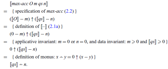
The proof for the other base case is similar.
Inductive case: we factor out the larger of the differences, ${(\textit{p}\mathbin{-}\textit{m})\mathbin{\uparrow}(\textit{q}\mathbin{-}\textit{n})}$
, to form the first part, and then work towards a situation where we can apply the specification (2.2) from right to left. We reason
${(\textit{p}\mathbin{-}\textit{m})\mathbin{\uparrow}(\textit{q}\mathbin{-}\textit{n})}$
, to form the first part, and then work towards a situation where we can apply the specification (2.2) from right to left. We reason
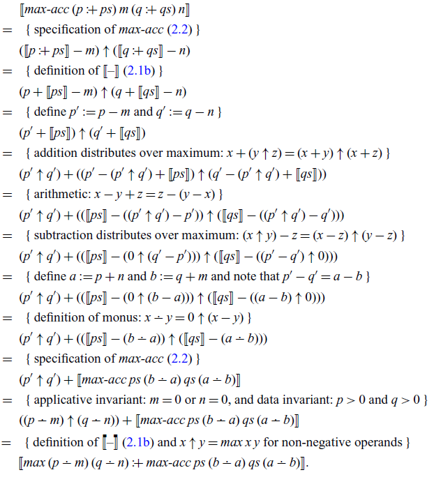
The final rewrites aim to avoid the use of integer subtraction in the body of max-acc. Finally, observe that the applicative invariant is maintained in the recursive call, as at least one of ${\textit{a}{\unicode{x2238}}\textit{b}}$
and
${\textit{a}{\unicode{x2238}}\textit{b}}$
and ${\textit{b}{\unicode{x2238}}\textit{a}}$
is zero.
${\textit{b}{\unicode{x2238}}\textit{a}}$
is zero.


 Open access
Discussions
No Discussions have been published for this article.