


1. Introduction
Wendelstein 7-X (W7-X) is the first stellarator that has been optimised for low neoclassical transport (Wolf Reference Wolf2008), besides other criteria. As such, it has been shown (Klinger et al. Reference Klinger, Andreeva, Bozhenkov, Brandt, Burhenn, Buttenschön, Fuchert, Geiger, Grulke and Laqua2019) that turbulence has become the limiting factor in the confinement for a broad range of its experiments. In order to understand the inherently nonlinear nature of plasma turbulence, numerical simulations based on gyrokinetic theory have become indispensable (Garbet et al. Reference Garbet, Idomura, Villard and Watanabe2010).
Using some of the world's most powerful supercomputers, it is possible nowadays to simulate gyrokinetic turbulence in stellarators globally, making it possible to take into account the full variation of the magnetic field on a flux surface while simultaneously considering its radial variations as well as temperature and density profiles – all of which are inherently impossible in flux-tube simulations. As such, studies like those of Navarro et al. (Reference Navarro, Merlo, Plunk, Xanthopoulos, von Stechow, Di Siena, Maurer, Hindenlang, Wilms and Jenko2020), Cole et al. (Reference Cole, Moritaka, Hager, Dominski, Ku and Chang2020), Sánchez et al. (Reference Sánchez, Mishchenko, García-Regaña, Kleiber, Bottino and Villard2020) and Wang et al. (Reference Wang, Holod, Lin, Bao, Fu, Liu, Nicolau, Spong and Xiao2020) have paved the way in investigating ion temperature gradient (ITG) turbulence globally in stellarators.
However, while these results already are of high importance, all of them relied on an adiabatic electron model, where only the ions were treated as a gyrokinetic particle species. This model fails to address things like trapped electron mode turbulence or the interaction between trapped electrons and ion turbulence, as well as electromagnetic effects, something that can become important for high-density operation of fusion devices.
All of these considerations motivated the upgrade of GENE-3D (Maurer et al. Reference Maurer, Navarro, Dannert, Restelli, Hindenlang, Görler, Told, Jarema, Merlo and Jenko2020), the extension of the widely established GENE framework (Jenko et al. Reference Jenko, Dorland, Kotschenreuther and Rogers2000) for three-dimensional magnetic field equilibria, to an electromagnetic gyrokinetic code, which is the focus of this work. In this paper, the underlying model of GENE-3D is presented, with special emphasis on the treatment of the electromagnetic terms in the gyrokinetic system of equations. Linear and nonlinear global verification studies using artificially heavy electrons to save computational cost against GENE are presented, showing excellent agreement between both codes, verifying the correctness and applicability of the electromagnetic upgrade. Finally, GENE-3D is used to perform global simulations of plasmas in W7-X with realistic electron mass and electromagnetic effects, something that, to the knowledge of the authors, has not been published before. It is found that, for the particular analytical background profiles used, the introduction of finite plasma-$\beta$ leads to a reduction in linear as well as nonlinear ITG strength.
The rest of the paper is structured as follows. The GENE-3D framework is introduced in § 2, highlighting the gyrokinetic model it uses and the numerical methods to solve the corresponding set of equations. In § 3, results of verification studies of the code against the global version of GENE in linear and nonlinear, electromagnetic tokamak simulations are presented, testing the correctness of the numerical implementation. In § 4, the first global, nonlinear gyrokinetic simulations of W7-X incorporating kinetic electrons with realistic mass, as well as electromagnetic effects are discussed. Finally, the main results of this paper are summarised in § 5 and an outlook for future projects is given.
2. Extending GENE-3D to an electromagnetic code
This section focuses on the algorithmic details of the extension of GENE-3D to include effects of a perturbed parallel vector potential. First, a brief overview of the gyrokinetic system of equations is given in § 2.1, followed by details specific to the implementation in § 2.2. Finally, additional information about the numerics of the code is presented in Appendix A.
2.1. Gyrokinetic Vlasov–Maxwell system
The GENE-3D code is a Eulerian code that solves the gyrokinetic Vlasov equation, coupled to Maxwell's equations (e.g. Brizard & Hahm Reference Brizard and Hahm2007) on a five-dimensional grid in phase space, using two velocity dimensions – the velocity parallel to the equilibrium magnetic field $v_{||}$ and the magnetic moment $\mu =mv_{\perp }^2/2B_0$
 – and three spatial dimensions $(x,y,z)$
 , representing a field-aligned coordinate system (Beer, Cowley & Hammett Reference Beer, Cowley and Hammett1995). Furthermore, it employs the so-called ‘$\delta f$
 ’ splitting (e.g. Garbet et al. (Reference Garbet, Idomura, Villard and Watanabe2010), and references therein). In this approach, one assumes that the full gyrocentre distribution function $F_{{\sigma }}$
 of species $\sigma$
 can be split into a stationary background distribution function $F_{0,\sigma }$
 , describing the plasma at thermal equilibrium, and a time-dependent, first-order perturbation $F_{1,\sigma }$
 :
:

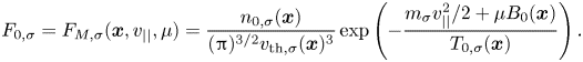
where $\epsilon _{\delta }$ is a smallness parameter describing the scale relation between background and perturbed quantities. The GENE-3D code assumes that the background distribution is given by a local Maxwellian:
Here, $m_{\sigma }$ , $n_{0,\sigma }$
 and $T_{0,\sigma }$
 are the mass, equilibrium background density and temperature of particle species $\sigma$
 at position ${\boldsymbol {x}}$
 , respectively. Furthermore, $B_0$
 gives the strength of the equilibrium magnetic field, $v_{||}$
 and $\mu$
 denote the velocity parallel to the magnetic field and the magnetic moment, respectively, and $v_{\textrm {th},\sigma }=\sqrt {2T_{0,\sigma }({\boldsymbol {x}})/m_{\sigma }}$
 is the thermal velocity of particle species $\sigma$
 . Under this assumption, the gyrokinetic equation for particle species $\sigma$
 , including a perturbation of the parallel vector potential, can be written as

where $\chi = \phi _1 - v_{||} A_{1,||}/c$ is called the gyrokinetic potential. The operator $\mathcal {G}\{ . \}$
 defines the forward-gyroaverage operator
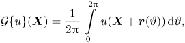
where $\boldsymbol {X}$ denotes the gyrocentre position and $\boldsymbol {r}$
 is the gyroradius vector orthogonal to the local magnetic field. The drift velocities appearing in (2.3) are defined as follows:
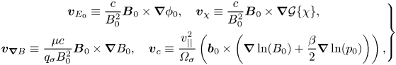
where $\varOmega _{\sigma } =(q_{\sigma } B_0)/(m_{\sigma } c)$ is the gyrofrequency of species $\sigma$
 , $\boldsymbol {b}_0=\boldsymbol {B}_0/B_0$
 is the unit vector in the direction of the equilibrium magnetic field $\boldsymbol {B}_0$
 , $p_0$
 is the equilibrium thermodynamic pressure, $\beta =8 {\rm \pi}p_0/B_0^2$
 is the ratio between plasma pressure and magnetic field strength and $c$
 is the speed of light.
At the current stage, GENE-3D uses a linearised Landau–Boltzmann collision operator for $C[F_{1,\sigma }]$ . Furthermore, the interplay between neoclassical and gyrokinetic physics is represented by the term coupling the curvature and $\boldsymbol {\nabla } B$
 drifts to the background Maxwellian (Oberparleiter et al. Reference Oberparleiter, Jenko, Told, Doerk and Görler2016), and the effects of a long-wavelength, radial electric field on the system (Helander & Simakov Reference Helander and Simakov2008; Mishchenko & Kleiber Reference Mishchenko and Kleiber2012) are represented by the term proportional to $\boldsymbol {v}_{E_0}$
 in (2.3). Though they are incorporated in the main algorithm, these effects are neglected in the simulations presented in this paper for simplicity.
The system is closed by the gyrokinetic field equations. Poisson's equation, providing the electrostatic potential, reads
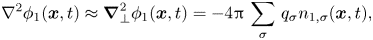
where only the spatial derivatives perpendicular to the magnetic field are retained, which is in accordance with the gyrokinetic ordering. In order to calculate the density perturbation at the particle position $\boldsymbol {x}$ from the gyrocentre position $\boldsymbol {X}$
 , GENE-3D employs a first-order pull-back transformation (e.g. Brizard & Hahm Reference Brizard and Hahm2007):

The operator $\mathcal {K}\{ . \}$ denotes the backward-gyroaverage operator, which is defined here as

Assuming a quasi-neutral limit ($\boldsymbol {\nabla }_{\perp }^2 \phi _1 \approx 0$ ), Poisson's equation can be rewritten as

At the current stage, magnetic compressibility, associated with a parallel perturbation of the magnetic field, is neglected, so that only the parallel vector potential $A_{1,||}$ is retained in GENE-3D, which is determined by the parallel component of Ampere's law:

self-consistently with the gyrokinetic equation and Poisson's equation.
2.2. Electromagnetic model
Although (2.3), (2.9) and (2.10) are an analytically closed system, particular care has to be taken of the term containing the partial time derivative of $A_{1,||}$ in (2.3). The approach used in GENE for a long time was to introduce a new distribution function $g_{\sigma }=F_{1,\sigma }+(q_{\sigma } v_{||} F_{M,\sigma } A_{1,||})/( T_{0,\sigma } c )$
 and solving the corresponding gyrokinetic system for $g_{\sigma }$
 instead of $F_{1,\sigma }$
 (Görler et al. Reference Görler, Lapillonne, Brunner, Dannert, Jenko, Merz and Told2011). However, it was shown in Crandall (Reference Crandall2019), that such a scheme becomes numerically unstable in nonlinear simulations at high plasma-$\beta$
 , although being stable linearly. In the same publication, an alternative scheme was proposed, similar to the one presented in Reynders (Reference Reynders1993), which has been included in the standard version of GENE recently. This scheme is also used in GENE-3D and is presented in the following. By defining the parallel inductive electric field as
one can rewrite the gyrokinetic equation in the form

where the term $R_{\sigma }$ contains all the contributions to the right-hand side of the gyrokinetic equation (2.3), except the one accounting for the parallel inductive electric field, and reads
The next step is to take the partial time derivative of Ampere's law (2.10) and multiply by $(-1/c)$ :
:

Inserting definition (2.12) into (2.14) eliminates the explicit coupling of the equation to the particle distribution function $F_{1,\sigma }$ . Therefore, one obtains an equation that treats the inductive electric field as an independent electromagnetic field:

Using (2.9), (2.10), (2.12), (2.13) and (2.15), the evolution of the distribution function $F_{1,\sigma }$ can be calculated by treating time as a discrete variable and using a numerical scheme to solve (2.12) in the above system approximately. For this, GENE-3D provides several explicit Runge–Kutta schemes, with a fourth-order-accurate Runge–Kutta scheme (RK4) being the default option.
3. Code verification
Having introduced the major changes performed to the GENE-3D code, the following subsections focus on comparing its results of global, electromagnetic tokamak simulations with those obtained from GENE. As the implementation of the electromagnetic terms in the gyrokinetic equation is independent of the field geometry, these cases provide a simple scenario for code validation. Benchmarks with other stellarator codes capable of performing electromagnetic simulations are left for future work.
3.1. Linear simulations with varying plasma-$\beta$

This subsection presents a linear verification study between GENE-3D and GENE over a large range of plasma pressures. For this, linear growth rates and mode frequencies of the most unstable mode are calculated varying the plasma-$\beta$ and are compared with the results presented in Görler et al. (Reference Görler, Tronko, Hornsby, Bottino, Kleiber, Norscini, Grandgirard, Jenko and Sonnendrücker2016).
The geometry is a tokamak with circular, concentric flux surfaces, with a magnetic field strength of $B_{0}=2.0\ \mathrm {T}$ on axis, which is called $B_{\textrm {ref}}$
 in the following, a major radius of $R_0=1.67\ \mathrm {m}$
 , an inverse aspect ratio of $a/R_0=0.36$
 and a safety factor profile

Furthermore, density and temperature profiles are defined according to
for both electrons and ions, where $A=(n,T_{i},T_{e})$ . The corresponding normalised gradients are

with $T(x_0)=2.14\ \mathrm {keV}$ , where $x_0/R_0=0.5$
 is the position at which the gradients have their maximum. The density at position $x_0$
 is adjusted to obtain the desired value of the reference plasma $\beta (x_0)=8{\rm \pi} n(x_0)T(x_0)/B_{\textrm {ref}}^2$
 . The parameters $\kappa _{A}$
 and $w_{A}$
 set the amplitude and the width of the gradients, respectively, and are chosen to be $\kappa _{T_i}=\kappa _{T_e}=6.96$
 , $w_{T_i}=w_{T_e}=0.3$
 , $\kappa _{n_i}=\kappa _{n_e}=2.23$
 and $w_{n_i}=w_{n_e}=0.3$
 . The box lengths are chosen to be $(L_{x},L_{v_{||}},L_{\mu })=(80\, \rho _{s},3\,v_{\textrm {th},\sigma } ,9\, T_{0,\sigma }(x_0)/B_{\textrm {ref}})$
 and $L_{y}=21.13\, \rho _{s}$
 , which results in resolving multiples of the toroidal mode number $n_0=19$
 . Here, $\rho _{s}=c_{s}/\varOmega _{s}$
 is the ion sound Larmor radius at reference position $x_0$
 . The simulation is performed using deuterium as ionic species, as well as electrons that have twice their realistic mass. The resolution at which GENE-3D converged is $(1344\times 16\times 16\times 64\times 32)$
 in $(x,y,z,v_{||},\mu )$
 , respectively, and hyperdiffusion was set as $\eta _{x}=2.0$
 , $\eta _{y}=0.05$
 , $\eta _{z}=2.0$
 and $\eta _{v_{||}}=0.2$
 . As is mentioned in Appendix A, periodic boundary conditions are employed in the bi-normal direction, whereas zero-valued Dirichlet boundary conditions are used for the radial domain. In order to avoid numerical instabilities caused by the fixed boundaries, buffer zones with a Krook damping operator are used at the radial boundaries, each covering 5 % of the domain.
Figure 1(a) shows the growth rate $\gamma$ of the dominant linear instability as a function of $\beta$
 , whereas figure 1(b) shows the frequency $\omega$
 of the respective mode. The red lines indicate the results obtained from GENE, whereas blue represents the results of GENE-3D. Excellent agreement is found for both frequencies and growth rates as the relative difference between the results of both codes is below 3 % in all cases. In particular, one can observe the expected stabilisation of the ITG mode by increasing $\beta$
 for both codes, as the growth rate decreases for $\beta$
 between 0.5 % and 1.4 %, while the frequency changes only slightly in the same interval. For values of $\beta$
 between 1.4 % and 1.75 % one can observe a transition of dominant modes from an ITG mode to a kinetic ballooning mode (KBM), which can be identified by the rapid increase in the mode frequency. The results for this interval are only shown here for the GENE code, since resolving this transition requires a much higher resolution than the one that was already used, which makes it impractical to investigate it with GENE-3D. Increasing $\beta$
 further results in an amplification of the KBM growth rate, while simultaneously causing a moderate decrease in its frequency, as observed with both codes. Finally, the radial and poloidal structures of the KBM at $\beta =2.5\,\%$
 are compared in figure 2, again showing excellent agreement between both codes.
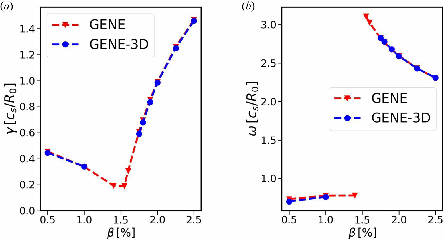
Figure 1. Linear growth rates (a) and mode frequencies (b) of the $n_0=19$ mode as a function of $\beta$
 . Red shows the results obtained from GENE, blue those from GENE-3D.
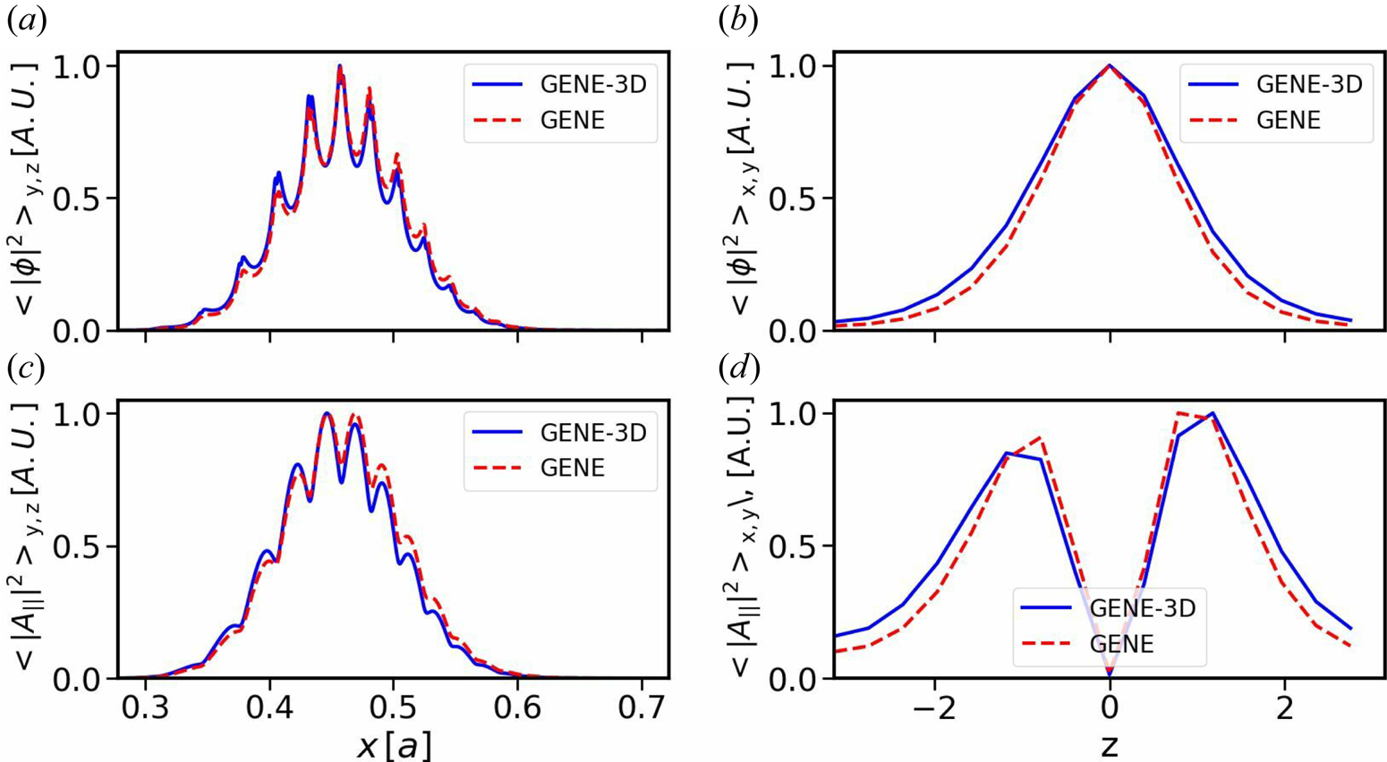
Figure 2. Normalised squares of the electrostatic and parallel vector potential for the scenario using $\beta =2.5\,\%$ . Radial (a) and poloidal (b) structures of the electrostatic potential, and radial (c) and poloidal (d) structures of the parallel vector potential. The red dashed line shows the results obtained from GENE, the blue solid line those from GENE-3D.
3.2. Nonlinear turbulence at finite plasma-$\beta$ in a tokamak

While the geometry being used is kept the same, it is beneficial for a nonlinear comparison to choose a broader profile than the one used in the previous subsection, as there is less unwanted profile relaxation in a gradient-driven approach with GENE-3D. Therefore, new plasma profiles of the form

are chosen, with $x_0/R_0=0.5$ , $\kappa _{T_i}=\kappa _{T_e}= 6.66$
 , $\kappa _n=2.20$
 , $w_{T_i}=w_{T_e}=w_{n}=0.04$
 and $\varDelta _{T_i}=\varDelta _{T_e}=\varDelta _{n}=0.8$
 . Furthermore, the plasma pressure is such that $\beta _{e}(x_0)=0.75\,\%$
 . In order to save computational time, the simulations were performed further increasing the electron-to-ion mass ratio to $m_{e}/m_{i}=0.01$
 and a finite-size parameter $\rho ^*_{s}=\rho _{s}/L_{\textrm {ref}}=\rho _{s}/R_0= 0.01$
 . The simulation covers the radial domain $0.1\leqslant x/R_0 \leqslant 0.9$
 , using buffer zones of 10 % at each side, with normalised box sizes being $(L_{x},L_{y},L_{v_{||}},L_{\mu })=(80.0\,\rho _{s},111.4 \,\rho _{s},3\, v_{\textrm {th},\sigma },9\, T_{0,\sigma }(x_0)/B_{\textrm {ref}})$
 and a resolution of $(n_{x},n_{k_y},n_{z},n_{v_{||}},n_{\mu })=(160\times 64\times 24\times 64\times 24)$
 for GENE and $(n_{x},n_{y},n_{z},n_{v_{||}},n_{\mu })=(160\times 256\times 24\times 64\times 24)$
 for GENE-3D. Finally, heat and particle sources, which are explained in Appendix A, were added with amplitudes being $\kappa _{H}=\kappa _{P}=0.1$
 and hyperdiffusion was set as $\eta _{x}=\eta _{y}=0.05$
 , $\eta _{z}=2.0$
 and $\eta _{v_{||}}=0.2$
 .
.
In order to compare the results of the two nonlinear simulations, the heat fluxes $Q_{\sigma }$ for species $\sigma$
 are considered in the following. The heat flux itself can be split into an electrostatic and an electromagnetic component, $Q_{\sigma }=Q_{\textrm {es},\sigma } +Q_{\textrm {em},\sigma }$
 , which are defined as

and

respectively, with

Here, $F_{1,\sigma }^{\textrm {particle}}$ is the perturbed distribution function of species $\sigma$
 , evaluated at particle position.
Figure 3 shows the volume-averaged time traces of the ion and electron heat flux contributions. The fluxes are time-averaged over the interval $t\in [100,345]R_0/c_{s}$ , which roughly contains the same number of burst, as follows. The time traces are divided in disjoint intervals each approximately three autocorrelation times long. An average over each one of them is performed, the result of which is then used to compute an ensemble mean and variance of the heat flux. The results are presented in table 1. Both simulations are in good agreement with each other, as the relative difference between their respective ensemble mean values is below 10 % for all components.
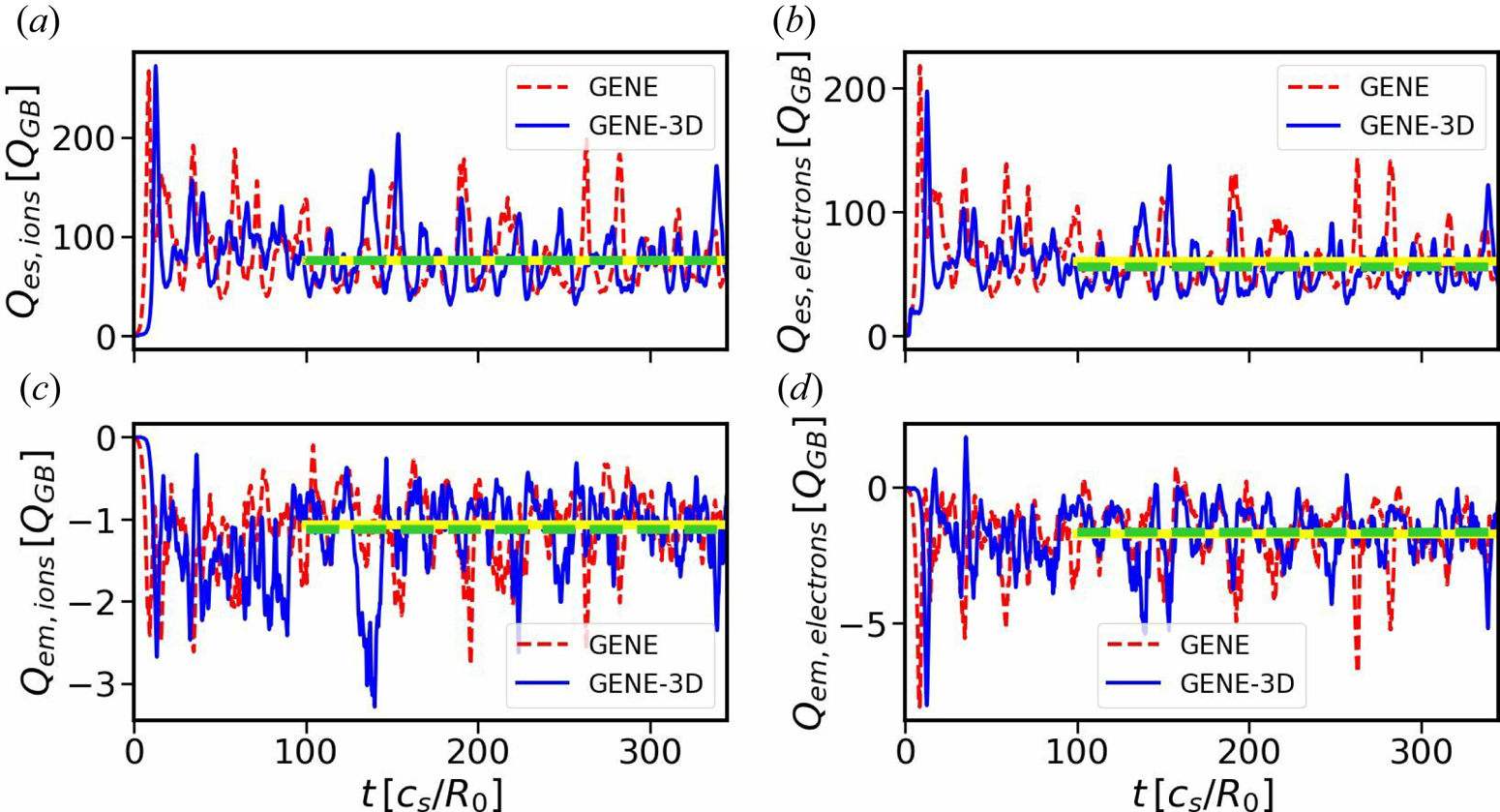
Figure 3. Time traces of the volume-averaged electron and ion heat fluxes. Yellow and green lines indicate average over the given time interval for GENE and GENE-3D, respectively. Electrostatic heat flux of ions (a) and electrons (b), and electromagnetic heat flux of ions (c) and electrons (d).
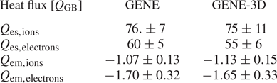
Table 1. Time-averaged heat flux contributions of GENE and GENE-3D.
The radial profiles of the heat flux contributions, averaged over a flux surface and in time, shown in figure 4, recover reasonable agreement between both codes as well. Here GENE and GENE-3D produce similar heat flux profiles, where ion and electron contributions are comparable in their magnitude. For both particle species, the fluxes are dominated by the electrostatic contribution, peaking around $x/R_0=0.6$ . At this position, GENE calculates heat fluxes of $Q_{\textrm {es},\textrm {ions}}=103.24\, Q_{\textrm {GB}}$
 and $Q_{\textrm {es},\textrm {electrons}}=80.09\, Q_{\textrm {GB}}$
 , whereas GENE-3D gives $Q_{\textrm {es},\textrm {ions}}=104.72\, Q_{\textrm {GB}}$
 and $Q_{\textrm {es},\textrm {electrons}}=75.41\, Q_{\textrm {GB}}$
 . Both results differ by less than $6\,\%$
 , giving additional confidence in the numerical implementation of GENE-3D. Finally, the spectra of the electrostatic heat fluxes at $x/R_0=0.6$
 are compared in figure 5. There are some small deviations between the heat flux spectra of both codes at the smallest scale, which is the result of the different representations of the bi-normal coordinate. Nevertheless, there is excellent agreement of the spectra in the wavenumber interval where most of the transport is located. Therefore, overall the linear as well as nonlinear verification studies of GENE-3D can be considered successful.
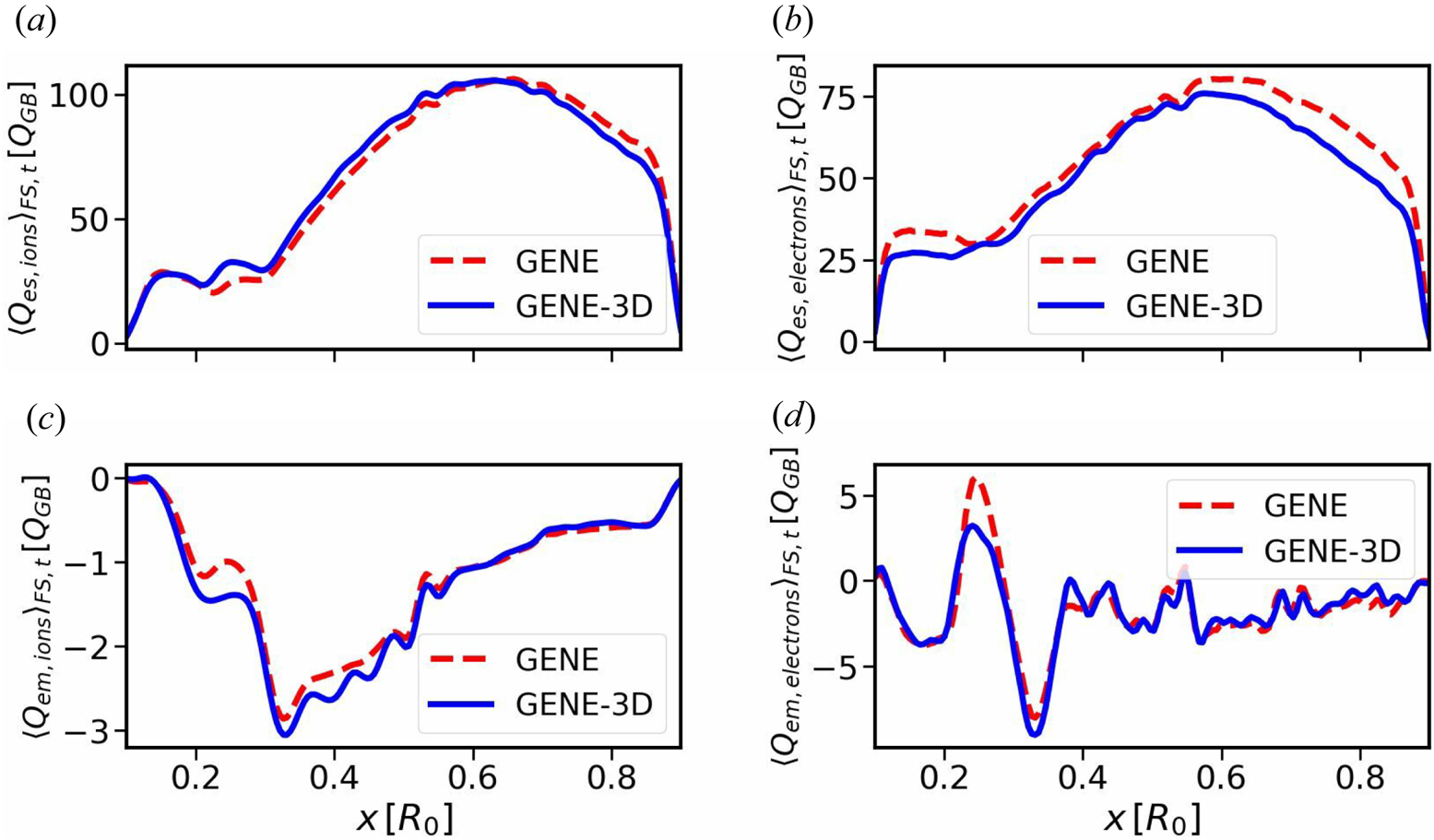
Figure 4. Radial profiles of heat flux contributions. Electrostatic heat flux of ions (a) and electrons (b), and electromagnetic heat flux of ions (c) and electrons (d).
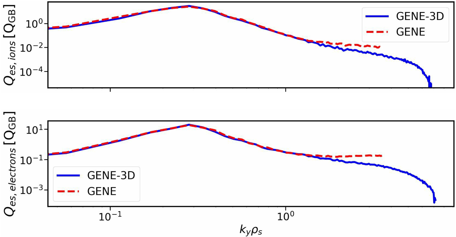
Figure 5. The $k_{y}$ spectra of the electrostatic heat fluxes, evaluated at $x/R_0=0.6$
 .
.
4. Electromagnetic effects on ITG turbulence in W7-X
Motivated by the successful verification in axisymmetric scenarios, electromagnetic simulations of W7-X are presented in this section. As the aim is to address the effect of finite plasma-$\beta$ on ITG turbulence (Snyder & Hammett Reference Snyder and Hammett2001) in W7-X, kinetic electron simulations in the electrostatic limit of $\beta _{e}(x_0)=10^{-4}$
 and electromagnetic simulations with $\beta _{e}(x_0)=0.5\,\%$
 were performed.
The profiles shown in figure 6 were used for all simulations discussed in this section. The variation of plasma-$\beta$ was achieved by varying the reference density $n_{\textrm {ref}}$
 . The specific choice of profiles localises turbulence in the centre of the plasma volume, such that one does not need to simulate the entire radial domain, with significant computational savings. The profiles are chosen to destabilise ITG modes by setting $\eta _{i}=L_{n}/L_{T_i}>1$
 and $\eta _{e}=L_{n}/L_{T_e}=1$
 . The specific form of the profiles is given by (3.4), with the defining parameters set to $\kappa _{T_i}= 4.0$
 , $\kappa _{T_e}=1.0$
 , $w_{T_i}=w_{T_e}=0.04$
 , $\varDelta _{T_i}=\varDelta _{T_e}=0.17$
 , $\kappa _{n}=1.0$
 , $w_{n}=0.04$
 and $\varDelta _{n}=0.17$
 . For both cases, the standard configuration of W7-X was used, where the specific geometries were generated with GVEC (Hindenlang et al. Reference Hindenlang, Maj, Strumberger, Rampp and Sonnendrücker2019) to be consistent with the background profiles and the prescribed plasma pressures. The reference temperature is $T(x_0)=4.0\ \mathrm {keV}$
 with $x_0/a=0.5$
 . The plasma is a hydrogen plasma with realistic electron mass. Together with the reference values of $B_{\textrm {ref}}=2.28\ \mathrm {T}$
 and $L_{\textrm {ref}}=a=0.52\ \mathrm {m}$
 this corresponds to a finite-size parameter $\rho ^*_{s}=\rho _{s}/a=1/184$
 . Furthermore, the radial domain $0.25\leqslant x/a \leqslant 0.75$
 was considered, using buffer zones covering 10 % of each side of the radial domain. Finally, it should be mentioned that the following simulations exploit the five-fold symmetry of W7-X by only considering one fifth of the toroidal domain.
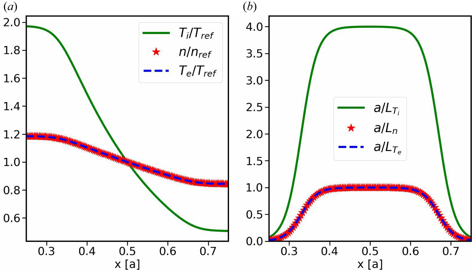
Figure 6. (a) Initial density and temperature profiles. (b) Initial density and temperature gradient profiles.
Linear simulations were performed to compare the growth rates of both scenarios. Since GENE-3D does not use a Fourier representation of the bi-normal direction, all modes are coupled and an initial value calculation will always only resolve the fastest growing mode present in the system. To overcome this issue, one can lower the bi-normal resolution to a point where said mode is no longer resolved, while still properly resolving the magnetic field geometry. While this method is not able to resolve local minima in the linear growth rate spectrum, it serves as a tool to calculate the maximum growth rate present in the system. An alternative is to use a numerical filter to single out the desired mode, as is done, for example, in the EUTERPE code. This is currently not implemented in GENE-3D, but it was shown in Sánchez et al. (Reference Sánchez, García-Regaña, Navarro, Proll, Moreno, González-Jerez, Calvo, Kleiber, Riemann and Smoniewski2021) that both methods are valid approaches. Three simulations were performed for each case, using a resolution of $(120\times 128\times 64\times 24)$ points in $(x,z,v_{||}, \mu )$
 , with box lengths of size $(L_{x},L_{\textrm {y}},L_{{\rm v}_{||}},L_{\mu })=(92.22\,\rho _{s},100.64 \,\rho _{s},4.2\, v_{\textrm {th},\sigma },17.7\, T_{0,\sigma }(x_0)/B_{\textrm {ref}})$
 and hyperdiffusion parameters $\eta _{x}=\eta _{y}=0.05$
 , $\eta _{ z}=2.0$
 and $\eta_{v_{||}}=0.2$
 . The bi-normal resolution was set to $(48,75,240)$
 , respectively, to resolve different linear modes. The corresponding growth rates are shown in figure 7, indicating a clear decrease induced by electromagnetic effects. The precise numerical values are listed in table 2, together with the ratio between the ion and electron heat fluxes, which is used later for comparison with the nonlinear results. One observes a reduction of the growth rates of approximately 20–25 %, with the maximum growth rate being decreased from $0.231{c_{s}/a}$
 to $0.179{c_{s}/a}$
 . For completeness, the radial and poloidal mode structures of the fastest-growing modes of both scenarios are compared in figure 8. Here one can observe that all fields peak radially close to $x/a=0.6$
 , with only a slight shift between the electrostatic and the electromagnetic cases. Furthermore, while the electrostatic potential is highly localised around $z=0$
 in both cases, the parallel vector potential of the electromagnetic simulation extends over the entire poloidal domain.
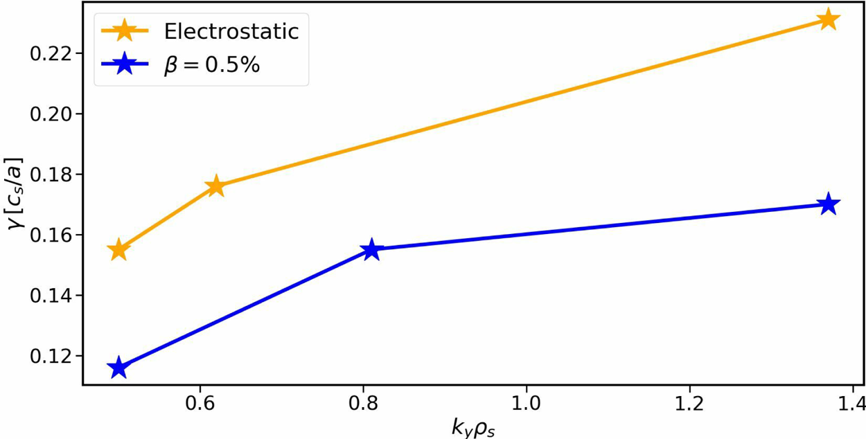
Figure 7. Linear growth rates as a function of the bi-normal wavenumber of both electrostatic and electromagnetic cases.
Table 2. Linear results of electrostatic and electromagnetic W7-X simulations.
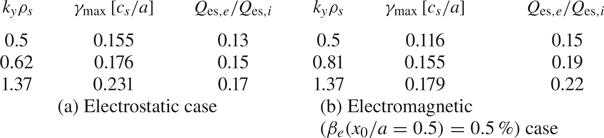
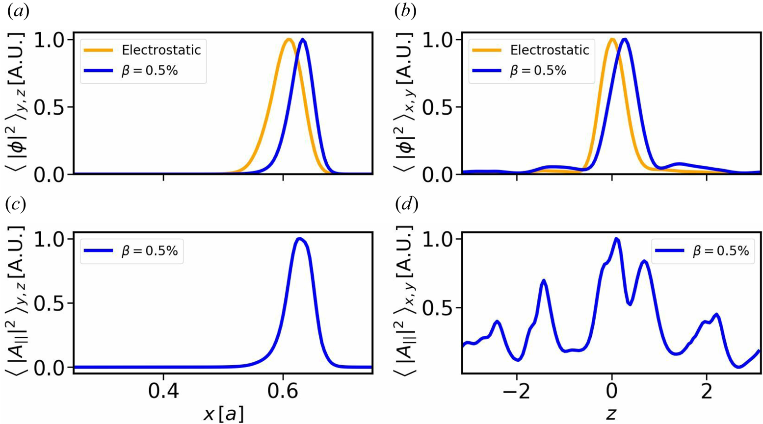
Figure 8. Normalised squares of the electrostatic and parallel vector potential of the fastest-growing modes for the electrostatic and electromagnetic scenarios. Radial (a) and poloidal (b) structures of the electrostatic potential, and radial (c) and poloidal (d) structures of the parallel vector potential. The orange lines show the structures of the electrostatic simulation, whereas the blue lines correspond to those of the electromagnetic set-up.
The stabilising properties of electromagnetic effects that were shown linearly can also be found in nonlinear simulations. For this, two simulations with the same parameters as for the linear cases were performed, except the resolution in $y$ , which was set to $n_{y}=120$
 . The cost of each simulation was around 700 000 CPU hours on the Intel Xeon Gold 6148 processors of the MPCDF cluster Cobra.
Figure 9 shows the volume-averaged time traces of the heat fluxes of both electrostatic and electromagnetic simulations. After approximately 200 time units, at which saturation is achieved, the electromagnetic case shows lower levels of turbulent heat fluxes than the electrostatic one. These differences in transport do not arise from nonlinear profile relaxation, but reflect the reduction of the linear growth rates, as can be seen in figure 10. In order to retain the background profiles, heat and particle sources of $\kappa _{H}=\kappa _{P}=0.03$ were used for both simulations, resulting in nearly identical profiles for both cases, with only minor deviations from the initial ones.
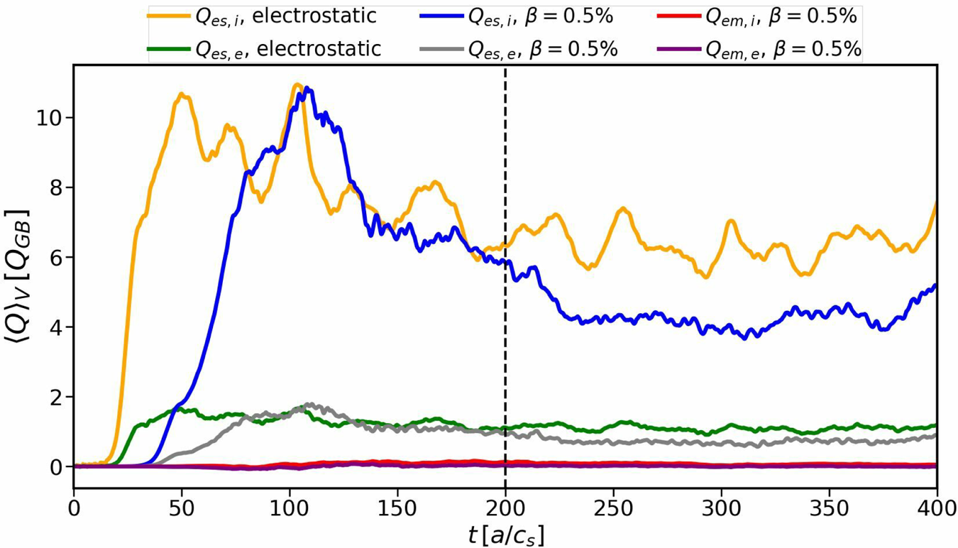
Figure 9. Time traces of the volume-averaged heat fluxes; the dashed black line indicates the beginning of the time interval used for averaging.
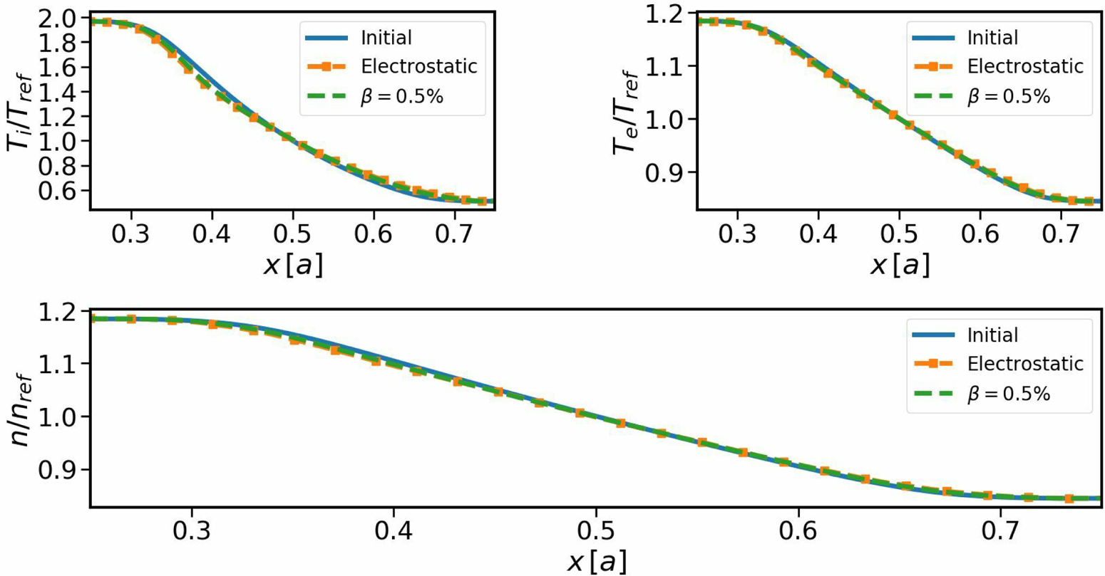
Figure 10. Time average of the background density and temperature profiles.
In order to elaborate further on the quantitative differences in transport between both scenarios, one can compare the radial profiles of the total electrostatic and electromagnetic heat fluxes, as shown in figure 11(a). One can easily see that the total electrostatic heat flux dominates the electromagnetic component with a peak value of $11.99{Q_{\textrm {GB}}}$ , in comparison with the maximum electromagnetic heat flux of $0.36{Q_{\textrm {GB}}}$
 . The electrostatic heat flux itself can again be split into contributions coming from the ions and the electrons and can then be compared individually. Figure 11(b) shows the radial profiles of the electrostatic heat fluxes of both scenarios, averaged over a flux surface and in time. The profiles are all peaking approximately at $x/a=0.46$
 . Both ions and electrons undergo a reduction of their turbulent heat fluxes through electromagnetic effects by approximately 25 %, with the peak ion heat flux being reduced from $13.70{Q_{\textrm {GB}}}$
 to $10.34{Q_{\textrm {GB}}}$
 and the electron flux from $2.25{Q_{\textrm {GB}}}$
 to $1.65{Q_{\textrm {GB}}}$
 . One should mention, however, that the aforementioned reduction is observed in gyro-Bohm units only, as the increase in the plasma-$\beta$
 is created by a 50-fold increase in the reference plasma density. This stabilisation is in line with the decrease in linear growth rates shown in table 2. One can further compare the relative magnitudes of ion and electron heat fluxes for both cases to see that they share a common ratio of approximately $Q_{\textrm {es},e}/Q_{\textrm {es},i}=0.15$
 . This is again similar to what was found in the linear simulations, although there seem to be slight deviations, especially for larger $k_{y}$
 in the electromagnetic simulation.
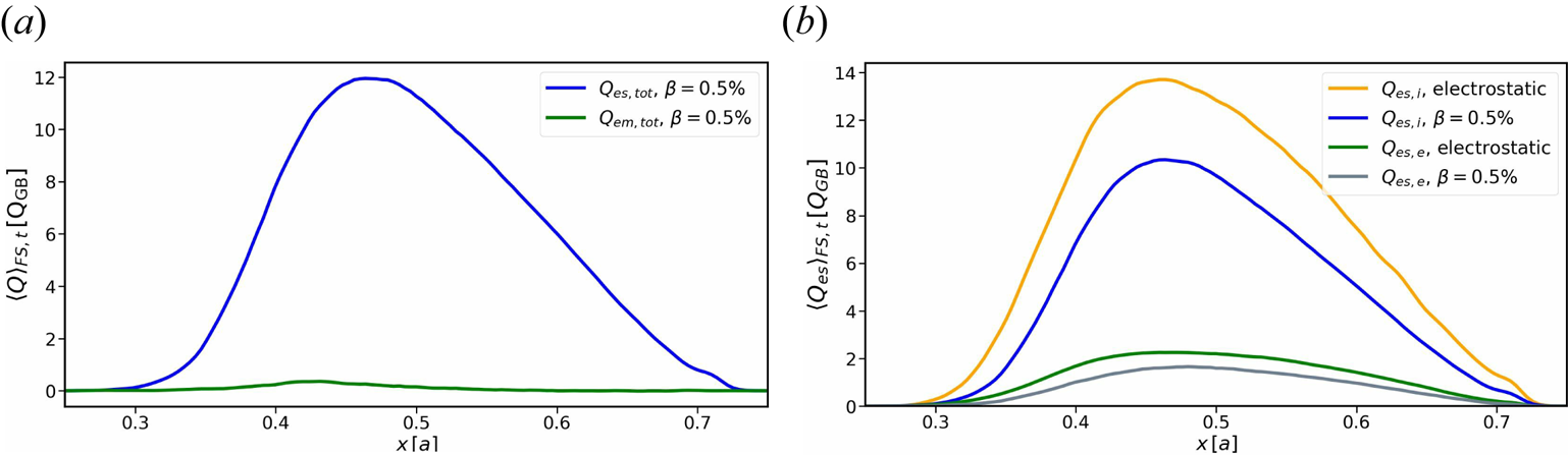
Figure 11. Time average of the radial heat flux profiles. (a) Electrostatic and electromagnetic heat fluxes and (b) electrostatic ion and electron heat fluxes.
To understand this, one has to take into account that not all modes contribute equally to turbulence, but that it is rather the low-$k_{y}$ modes that enter most, in particular for ITG turbulence, as was already shown, for example, in Navarro et al. (Reference Navarro, Merlo, Plunk, Xanthopoulos, von Stechow, Di Siena, Maurer, Hindenlang, Wilms and Jenko2020). To confirm this, the bi-normal wave spectra of the electrostatic heat fluxes at $x/a=0.46$
 are shown in figure 12. All the heat fluxes peak around $k_y\rho _{s} \sim 0.3$
 , which is below the smallest $k_{y}$
 that was resolved linearly, with only minor contributions from $k_{y} \rho _{s} \sim 1$
 and beyond.
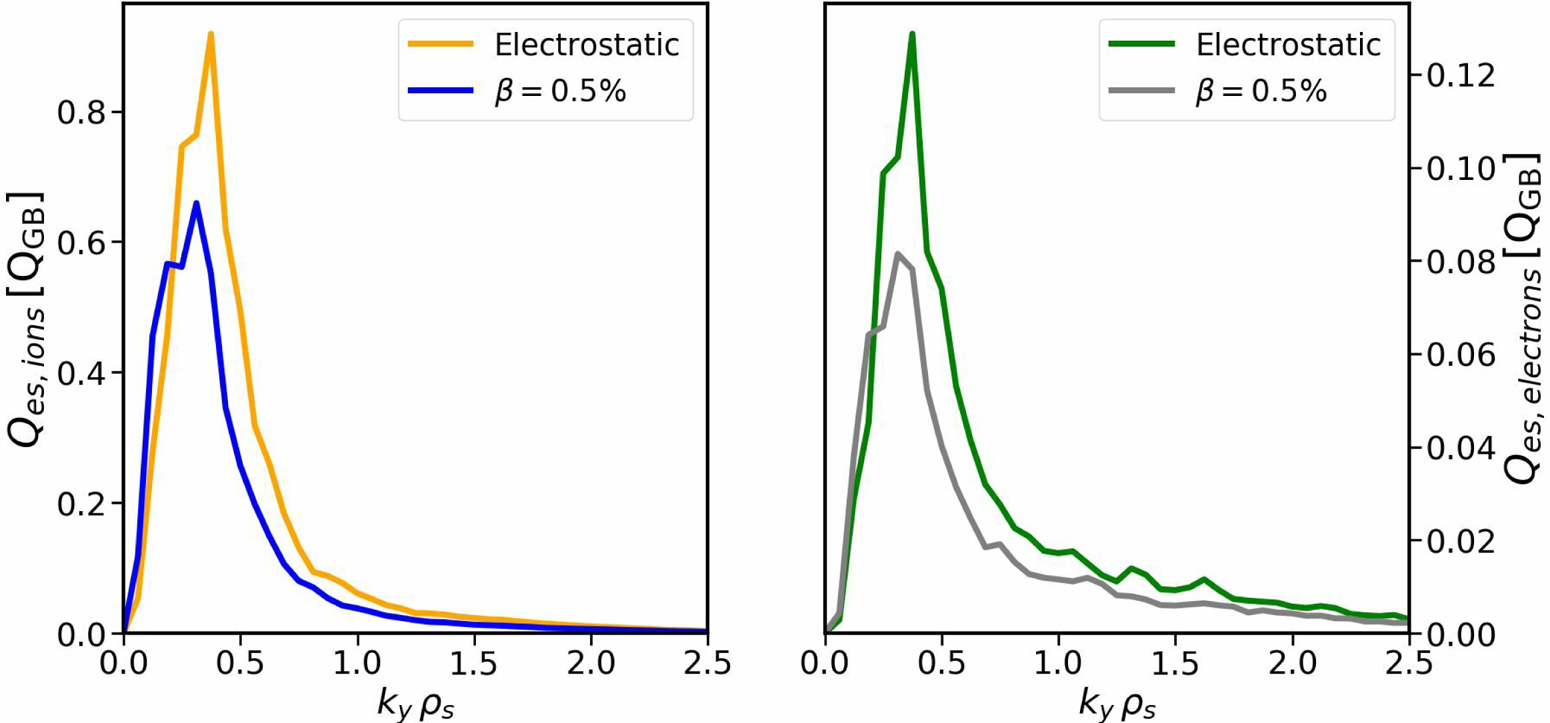
Figure 12. Wavenumber spectra of ionic and electronic electrostatic heat fluxes, evaluated at $x/a=0.46$ .
.
Overall, both linear and nonlinear simulations show a consistent reduction of ITG activity through electromagnetic effects for the given plasma-$\beta$ . Nevertheless, increasing $\beta$
 will eventually result in the excitation of KBM turbulence, similar to the transition shown in § 3.1, which highlights the importance of electromagnetic effects for future investigations.
5. Conclusion
The present paper focuses on the upgrade of the GENE-3D code to capture electromagnetic effects by retaining a perturbation in the parallel vector potential. The main extension to the numerical scheme of GENE-3D with respect to Maurer et al. (Reference Maurer, Navarro, Dannert, Restelli, Hindenlang, Görler, Told, Jarema, Merlo and Jenko2020) was the introduction of an additional field equation to compute the time derivative on the right-hand side of the gyrokinetic equation. Both linear and nonlinear verification studies show excellent agreement with the well-established tokamak code GENE, proving the correct implementation and viability of the electromagnetic upgrade.
The code was then applied to W7-X with the goal of addressing electromagnetic stabilisation of ITG turbulence. To this end, a set of analytical density and temperature profiles was considered in the standard configuration of W7-X. Linear and nonlinear simulations have been performed comparing the results between an electromagnetic case with $\beta _{e}(x/a)=0.5\,\%$ and a case in the electrostatic limit. Electromagnetic effects cause a reduction by 25 % of the linear growth rates, which in turn results in a similar reduction of the saturated nonlinear fluxes. While these results were obtained under simplifying assumptions, e.g. using analytical profiles and artificial reference parameters, they demonstrate that GENE-3D is able to perform electromagnetic simulations and that finite-$\beta$
 stabilisation can be important for stellarators as well.
In order to approach such applications without these constraints, realistic simulations of W7-X discharges are planned for the future. Furthermore, it will be of great interest to study electromagnetic instabilities in medium- to high-plasma-$\beta$ regimes in stellarators.
Acknowledgements
F.W. would like to thank K. Stimmel, T. Hayward-Schneider and D. Michels for many fruitful discussions, helpful suggestions and comments. Numerical simulations were performed at the MARCONI-Fusion supercomputer at Cineca, Italy, as well as at the Cobra and Raven HPC systems at the Max Planck Computing and Data Facility (MPCDF), Germany.
Editor Per Helander thanks the referees for their advice in evaluating this article.
Funding
This work has been carried out within the framework of the EUROfusion Consortium and has received funding from the Euratom research and training programme 2014–2018 and 2019–2020 under grant agreement no. 633053. The views and opinions expressed herein do not necessarily reflect those of the European Commission.
Declaration of interests
The authors report no conflict of interest.
Appendix A. Additional numerical details
This appendix briefly mentions some additional numerical details of GENE-3D, a detailed discussion of which can be found in Maurer et al. (Reference Maurer, Navarro, Dannert, Restelli, Hindenlang, Görler, Told, Jarema, Merlo and Jenko2020).
Phase-space variables are discretised in order to solve the gyrokinetic system numerically. For this, the velocity space parallel to the magnetic field lines is partitioned on an equidistant grid with zero Dirichlet boundaries, whereas the grid in the direction of the magnetic moment is distributed using a Gauss quadrature scheme with Gauss–Legendre weights and knots (Abramowitz & Stegun Reference Abramowitz and Stegun1965). For the spatial discretisation, the three field-aligned coordinates

are introduced. Here, $\rho _{\textrm {tor}}=\sqrt {\varPhi _{\textrm {tor}}/\varPhi _{\textrm {edge}}}$ is used as a radial coordinate, where $\varPhi _{\textrm {tor}}$
 is the toroidal flux and $\varPhi _{\textrm {edge}}$
 its value at the last closed flux surface. The bi-normal coordinate $y$
 is based on the field line label $\alpha =q(x) \theta ^*-\varphi$
 at a fixed flux surface, where $q(x)$
 is the safety factor, $\theta ^*$
 is the poloidal PEST angle (Li, Breizman & Zheng Reference Li, Breizman and Zheng2016), $\varphi$
 is the geometrical toroidal angle and the constant $C_{y}$
 is defined as $C_{y}=x_0/|q_0|$
 , where $q_0$
 is the safety factor at the reference point $x_0$
 . Lastly, the parallel coordinate $z$
 describes the position along a magnetic field line. In addition, the sign of the poloidal magnetic field $\sigma _{B_p}$
 ensures that the parallel direction is always in the direction of the magnetic field. The magnetic field, as well as other geometric coefficients, such as the safety factor profile and metric coefficients, are provided via an interface by the Galerkin Variational Equilibrium Code (GVEC), an ideal magnetohydrodynamics equilibrium solver which follows the ideas of the well-established VMEC code (Hirshman & Whitson Reference Hirshman and Whitson1983; Hirshman & Betancourt Reference Hirshman and Betancourt1991).
The spatial grids in GENE-3D themselves are rectangular, equidistant meshes, which makes it particularly easy to calculate spatial derivatives using a fourth-order-accurate central-difference scheme. The boundaries in the radial direction have zero-valued Dirichlet conditions. The bi-normal coordinate is treated periodically, whereas the well-established twist-and-shift boundary condition (Beer et al. Reference Beer, Cowley and Hammett1995) is used at the boundaries along a magnetic field line.
In order to avoid unphysical high-wavenumber modes that arise due to the central-difference approximations, one can introduce numerical hyperdiffusion terms to the right-hand side of the gyrokinetic equation to dampen these modes. The hyperdiffusion terms in the $x$ , $y$
, $y$ , $z$
, $z$ and $v_{||}$
 directions are all fourth-order-accurate terms with second-order stencils, meaning that they are of the form

where $u$ represents any of the previously mentioned coordinates and the damping parameter $\eta _{u}$
 can be set for each coordinate individually as input by the user.
By applying radial Dirichlet boundary conditions to the distribution functions, density and temperature profiles are fixed at the boundaries of the radial domain, which can cause strong turbulence and numerical instabilities at the boundaries. To avoid this, it is advisable to employ a Krook damping operator of the form

to the right-hand side of (2.12), where the damping factor $\nu (x)$ is implemented as a fourth-order polynomial with compact support within a buffer region at the radial boundaries, typically 5 %–10 % at each side of the domain (G��rler et al. Reference Görler, Lapillonne, Brunner, Dannert, Jenko, Merz and Told2011). As GENE-3D uses a gradient-driven approach (Görler et al. Reference Görler, Lapillonne, Brunner, Dannert, Jenko, Aghdam, Marcus, McMillan, Merz and Sauter2011; Rath et al. Reference Rath, Peeters, Buchholz, Grosshauser, Migliano, Weikl and Strintzi2016; Lanti et al. Reference Lanti, McMillan, Brunner, Ohana and Villard2018) so far, numerical particle and heat sources have to be introduced to the gyrokinetic equation (2.12) in order to maintain the density and temperature profiles. The sources are of the form

in the case of the particle source and

for the heat source. Here,
denotes the flux-surface average (D'haeseleer et al. Reference D'haeseleer, Hitchon, Callen and Shohet2012) and

The symmetrisation of the distribution function with respect to $v_{||}$ in (A5) ensures the conservation of parallel momentum and the terms proportional to $\langle \int \dots \rangle _{\textrm {FS}}/\langle \int \dots \rangle _{\textrm {FS}}$
 avoids the unwanted numerical injection of particles (McMillan et al. Reference McMillan, Jolliet, Tran, Villard, Bottino and Angelino2008). The coefficients $\kappa _{P}$
 and $\kappa _{H}$
 are specified by the user and should be chosen to be around 5 %–10 % of the maximum linear growth rate of the system (Lapillonne et al. Reference Lapillonne, McMillan, Görler, Brunner, Dannert, Jenko, Merz and Villard2010).
The nonlinear term in (2.13), coupling $\boldsymbol {v}_{\chi }$ to $F_{1,\sigma }$
 and $\phi _1$
 , can be written in the form

where the two-dimensional Poisson brackets for functions $A$ and $B$
 have been defined here as

An Arakawa scheme (Arakawa Reference Arakawa1997) is used to evaluate the Poisson brackets in (A8) numerically, as it ensures the conservation of free energy in nonlinear simulations (Bañón Navarro et al. Reference Bañón Navarro, Morel, Albrecht-Marc, Carati, Merz, Görler and Jenko2011).
Finally, in order to perform the gyroaverages efficiently, the distribution functions as well as the electromagnetic fields are discretised using a finite-element method in the directions perpendicular to the magnetic field, currently employing bicubic piecewise polynomials. Doing so, together with the finite-difference approximations of the derivatives, allows one to transform the field equations (2.9), (2.10) and (2.15) into a set of sparse, linear systems. This makes it possible to use the PETSc library (Balay et al. Reference Balay, Gropp, McInnes and Smith1997, Reference Balay, Abhyankar, Adams, Brown, Brune, Buschelman, Dalcin, Eijkhout, Gropp and Karpeyev2019) in order to solve the equations for the electromagnetic fields. While providing an extensive set of iterative solvers already, PETSc can also serve as an interface to direct solvers such as MUMPS (Amestoy et al. Reference Amestoy, Duff, L'Excellent and Koster2001, Reference Amestoy, Guermouche, L'Excellent and Pralet2006) or SuperLU_(Li & Demmel Reference Li and Demmel2003).


 Open access