


1 Introduction
Plasmas composed of relativistic electrons and positrons, also called pair plasmas, have garnered considerable interest due to their applicability in a variety of astrophysical and laboratory environments. Examples of this include accretion disks (Liang Reference Liang1979; White & Lightman Reference White and Lightman1989; Bjöernsson et al. Reference Bjöernsson, Abramowicz, Chen and Lasota1996), models of the early universe (Gibbons, Hawking & Siklos Reference Gibbons, Hawking and Siklos1983; Tajima & Taniuti Reference Tajima and Taniuti1990), active galactic nuclei (AGN) (Lightman & Zdziarski Reference Lightman and Zdziarski1987), pulsar magnetospheres (Curtis Reference Curtis1991; Istomin & Sobyanin Reference Istomin and Sobyanin2007), hypothetical quark stars (Usov Reference Usov1998) and in the laboratory recently, Sarri et al. (Reference Sarri, Poder, Cole, Schumaker, Di Piazza, Reville, Dzelzainis, Doria, Gizzi and Grittani2015) created ion-free electron–positron (EP) plasma by using a compact laser-driven set-up. The existence of a variety of nonlinear structures such as waves, solitons and instabilities is well established in these relativistic EP plasmas. Aside from this, magnetic self-organization or relaxation is another important phenomenon in magnetized laboratory and astrophysical plasmas. During the process of plasma relaxation, a plasma attains an equilibrium state by minimizing its energy under some topological constraints. This equilibrium state is called a relaxed or self-organized state. In the case of ideal magnetohydrodynamics (MHD), the relaxed state can be obtained by minimizing the magnetic energy subject to the magnetic helicity constraint. Specifically, the relaxed state corresponds to a single Beltrami field (a vector field whose vortex is collinear to itself) or state, which can be mathematically expressed as $\boldsymbol {\nabla }\times \boldsymbol {B}=\lambda \boldsymbol {B}$ , where $\boldsymbol {B}$
 denotes the magnetic field, $\lambda$
 is a constant, and the eigenvalue of the curl operator is referred to as the scale parameter. This single Beltrami relaxed state is force-free, flowless and devoid of pressure gradients. It is noteworthy that the entirety of the relaxed state structure's information, which includes its dimensions, nature, and shear or twist, is encompassed within $\lambda$
 (Woltjer Reference Woltjer1958; Taylor Reference Taylor1974).
Later, to obtain a more realistic and non-force-free relaxed state, Hall MHD (HMHD) was invoked instead of ideal MHD. For HMHD, the relaxed state is the double Beltrami (DB) state, which is the superposition of two single force-free states. The DB state is characterized by two scale parameters, and it also shows a strong magnetofluid coupling resulting in significant pressure gradients (Mahajan & Yoshida Reference Mahajan and Yoshida1998; Steinhauer Reference Steinhauer2002). In further studies, it was shown that the inertia of plasma species plays a significant role in the formation of multi-Beltrami relaxed state structures (Mahajan & Lingam Reference Mahajan and Lingam2015). In this regard, the relaxed state of an EP plasma is the triple Beltrami (TB) state. A TB state is a linear combination of three single Beltrami fields and is characterized by three scale parameters (Bhattacharyya, Janaki & Dasgupta Reference Bhattacharyya, Janaki and Dasgupta2003). While for a three-component plasma and when all the plasma species are inertial, the self-organized state is the quadruple Beltrami (QB) state – a linear combination of four single Beltrami fields with four self-organized structures (Shatashvili, Mahajan & Berezhiani Reference Shatashvili, Mahajan and Berezhiani2016). In recent years, such multi-Beltrami relaxed states have also been investigated by several researchers in relativistic hot EP (Iqbal, Berezhiani & Yoshida Reference Iqbal, Berezhiani and Yoshida2008), relativistic hot electron–positron–ion (EPI) (Iqbal & Shukla Reference Iqbal and Shukla2012, Reference Iqbal and Shukla2013; Shazad, Iqbal & Ullah Reference Shazad, Iqbal and Ullah2021; Shazad & Iqbal Reference Shazad and Iqbal2023), relativistic degenerate EPI (Shatashvili et al. Reference Shatashvili, Mahajan and Berezhiani2016) and relativistic degenerate two electron-temperature electron–ion plasmas (Shatashvili, Mahajan & Berezhiani Reference Shatashvili, Mahajan and Berezhiani2019).
The Beltrami states discussed above have also proven to be efficacious in plasma confinement (Mahajan & Yoshida Reference Mahajan and Yoshida1998) and the modelling of various aspects of magnetized plasmas in astrophysical phenomena. Some applications of Beltrami states in astrophysical phenomena are solar flares (Ohsaki et al. Reference Ohsaki, Shatashvili, Yoshida and Mahajan2002; Kagan & Mahajan Reference Kagan and Mahajan2010), solar arcades and loops (Bhattacharyya et al. Reference Bhattacharyya, Janaki, Dasgupta and Zank2007; Fuentes-Fernández, Parnell & Hood Reference Fuentes-Fernández, Parnell and Hood2010), coronal heating (Mahajan et al. Reference Mahajan, Miklaszewski, Nikol'skaya and Shatashvili2001; Browning & Van der Linden Reference Browning and Van der Linden2003), large-scale dynamo and reverse dynamo mechanisms (Mininni, Gómez & Mahajan Reference Mininni, Gómez and Mahajan2002; Mahajan et al. Reference Mahajan, Shatashvili, Mikeladze and Sigua2005; Kotorashvili, Revazashvili & Shatashvili Reference Kotorashvili, Revazashvili and Shatashvili2020; Kotorashvili & Shatashvili Reference Kotorashvili and Shatashvili2022), turbulence (Krishan Reference Krishan2004; Krishan & Mahajan Reference Krishan and Mahajan2004) and striped wind of pulsar nebula (Pino, Li & Mahajan Reference Pino, Li and Mahajan2010). Furthermore, the application of Beltrami states has also been expanded to encompass curved space–time, allowing for their utilization in the modelling of plasmas located in the vicinity of black holes as well as the early universe (Bhattacharjee et al. Reference Bhattacharjee, Das, Stark and Mahajan2015; Bhattacharjee, Feng & Stark Reference Bhattacharjee, Feng and Stark2018; Asenjo & Mahajan Reference Asenjo and Mahajan2019; Bhattacharjee Reference Bhattacharjee2020; Bhattacharjee & Feng Reference Bhattacharjee and Feng2020).
Recent years have seen a number of studies exploring the nonlinear interaction between photons and relativistic hot EP plasmas (Tajima & Taniuti Reference Tajima and Taniuti1990; Shukla Reference Shukla1993; Shukla, Tsintsadze & Tsintsadze Reference Shukla, Tsintsadze and Tsintsadze1993; Mendonça & Shukla Reference Mendonça and Shukla2008). However, the goal of the present work is to investigate the relaxation of relativistic EP plasma that is composed of inertial relativistic hot electrons and positrons in a massive photon field. Moreover, it is also crucial to mention that only relativistic temperature effects will be taken into account in this study. A plasma is considered relativistically hot if the thermal energy possessed by plasma particles is equal to or surpasses their rest mass energy. In the context of our plasma model it is important to explain that in classical electrodynamics, the photon is assumed to have zero mass (Goldhaber & Nieto Reference Goldhaber and Nieto1971; Tu, Luo & Gillies Reference Tu, Luo and Gillies2005; Goldhaber & Nieto Reference Goldhaber and Nieto2010; Jackson Reference Jackson2021). It is deduced from the condition that the Lagrangian describing the electromagnetic field must have gauge invariance. In the same vein as the cosmological constant and the masses of neutrinos, both of which were originally considered to be precisely zero until empirical evidence revealed otherwise, it is plausible to presume that a photon possesses a mass that is very small but not zero (Reece Reference Reece2019; Aghanim et al. Reference Aghanim, Akrami, Ashdown, Aumont, Baccigalupi, Ballardini, Banday, Barreiro, Bartolo and Basak2020). Research on dark matter, in which massive dark photons are postulated to be force carriers that can kinetically interact with the photon predicted by the standard model, is another factor that continues to pique interest in massive photons (Filippi & De Napoli Reference Filippi and De Napoli2020).
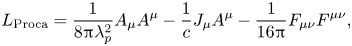
The electromagnetic field Lagrangian, first considered by Proca and also termed the Proca Lagrangian, can be modified to incorporate a mass term to account for photon mass that can be expressed as (Jackson Reference Jackson2021)
where $A_{\mu }$ , $J_{\mu }$
 , $F_{\mu \nu }$
 , $c$
, $c$ and $\lambda _{p}$
 ($h/m_{\nu }c,$
 in which $h$
 is Plank's constant and $m_{\nu }$
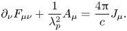
 is photon mass) are four potentials, four currents, electromagnetic field stress tensor, the speed of light and the Compton wavelength, respectively. This Proca Lagrangian leads to the following equation of motion for massive photons:
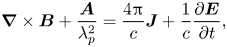
Some of the immediate repercussions of non-zero photon mass include wavelength dependence of the speed of light, departures from the exactness of Coulomb's and Ampere's laws, longitudinal polarization of electromagnetic waves, and Yukawa-like dependency of the magnetic field formed by a magnetic dipole (Goldhaber & Nieto Reference Goldhaber and Nieto1971; Bay & White Reference Bay and White1972; Rawls Reference Rawls1972; Tu et al. Reference Tu, Luo and Gillies2005; Goldhaber & Nieto Reference Goldhaber and Nieto2010). Similarly, a very important implication of non-zero photon mass is a modification of Ampere's law. For instance, Ampere's law in Maxwell–Proca electrodynamics can be expressed as (Ryutov Reference Ryutov1997)
where $\boldsymbol {B}$ , $\boldsymbol {E}$
 , $\boldsymbol {A}$
 and $\boldsymbol {J}$
 are magnetic field, electric field, vector potential and current density, respectively. Due to their extreme precision, photon mass measurements in laboratories have reached their limitations (Tu & Luo Reference Tu and Luo2004). The currently recognized upper limit for photon mass is $m_{\nu }\leq 10^{-49}$
 g and corresponding to this value $\lambda _{p}\geq 1$
 au (Adelberger, Dvali & Gruzinov Reference Adelberger, Dvali and Gruzinov2007; Particle Data Group 2022). Recently, in the context of magnetized plasmas, some specific solutions to the MHD equations that take into consideration the finite photon mass have been presented and studied in light of the prospect of refining the estimate of the photon mass based on a variety of astrophysical observations (Ryutov Reference Ryutov1997, Reference Ryutov2007, Reference Ryutov2009, Reference Ryutov2010). Moreover, Ryutov, Budker & Flambaum (Reference Ryutov, Budker and Flambaum2019) have also investigated the MHD plasma equilibrium to study the effect of Maxwell–Proca electromagnetic stresses on galactic rotation curves (Ryutov et al. Reference Ryutov, Budker and Flambaum2019). The study also suggests that standard theory of plasma relaxation (Woltjer Reference Woltjer1958; Taylor Reference Taylor1974) can also be extended to such plasma systems which incorporate the effect of non-zero photon mass, and for such plasma models magnetic vector potential $\boldsymbol {A}$
 also satisfies the Beltrami condition $\boldsymbol {\nabla }\times \boldsymbol {A}=\lambda \boldsymbol {A}$
 . Bhattacharjee (Reference Bhattacharjee2023) has recently advanced the concept of equilibrium states in terms of vector potential and obtained a TB state for a quasineutral single species plasma.
Due to the ubiquity of EP plasmas and their inherent self-organizing nature, which leads to the formation of coherent magnetic and flow patterns, it becomes crucial to investigate the plasma equilibria of relativistic hot EP plasmas. In the present work, a QB relaxed state equation for magnetic vector potential in relativistic hot EP plasma is derived by incorporating the effect of non-zero photon mass by considering it as a mobile fluid. The objective of this study is to examine the potential presence of Beltrami states at scales larger than the Compton wavelength and explore the variations that arise as a result of a non-zero photon mass. In contrast to the Beltrami state applicable to zero photon mass, the states under consideration predominantly involve the magnetic vector potential $\boldsymbol {A}$ due to its dynamic nature within the framework of massive electromagnetism. This study aims to address certain analytical challenges in the field of massive electromagnetism, specifically related to multi-Beltrami equilibria such as the upper mass limit for photons and galactic rotation curves.
To derive a QB relaxed state, first, vortex dynamics equations for pair species are derived from relativistic equations of motion, and then the steady-state solutions of vortex dynamics equations are coupled with a modified Ampere's law. This modified Ampere's law incorporates the effect of non-zero photon mass in Maxwell–Proca electrodynamics. Furthermore, the analysis of the relaxed state shows that all the scale parameters become real for higher relativistic temperatures and sub-Alfvénic flows of plasma species. These scale parameters also show the possibility of multiscale structure formation in this QB state. The size of one of the structures is greater than or equal to the Compton wavelength. While the size of one structure is greater than the electron skin depth, the dimensions of the remaining two structures are equal to or smaller than the electron skin depth. Additionally, an analytical solution of the QB field and flow is presented in an axisymmetric cylindrical geometry. The field profiles show that at lower relativistic temperatures, for given values of generalized helicities of plasma species, plasma shows a diamagnetic trend. Also, the field and flow profiles show the possibility for the formation of microscale energy reservoirs, which may be either kinetic or magnetic in nature. The existence of microscale energy reservoirs can be attributed to the multiscale structures present in the QB state, which have important implications for dynamo and reverse dynamo processes.
This paper is structured in the following manner. In § 2, from model equations, the QB relaxed state equation is derived. The general properties of the QB self-organized state are presented in § 3. In § 4, the analytical solution of the QB field and flow in an axisymmetric cylindrical geometry is presented. The summary of the present findings is given in § 5.
2 Model equations and the QB state
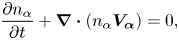
Consider a quasineutral and incompressible magnetized relativistic hot EP plasma in a massive photon field. In order to account for the effect of non-zero mass, we will use Maxwell–Proca electrodynamics. Now the continuity equation and relativistic equation of motion for $\alpha$ (electrons, e; positrons, p) plasma species are
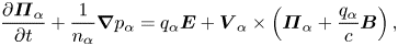
where $\boldsymbol {\varPi _{\alpha }}=m_{0\alpha }\gamma _{\alpha }G_{\alpha }\boldsymbol {V_{\alpha }}$ , $p_{\alpha }=n_{\alpha }T_{\alpha }/\gamma _{\alpha }$
 , $n_{\alpha }$
 , $m_{0\alpha }$
 , $\boldsymbol {V_{\alpha }}$
 , $\gamma _{\alpha }=1/\sqrt {1-(V_{\alpha }/c)^{2}}$
 , $T_{\alpha }$
 and $q_{\alpha }$
 are relativistic momentum, thermal pressure, number density, rest mass, velocity, relativistic Lorentz factor, temperature and electric charge of plasma species, respectively, while $\boldsymbol {E}$
 and $\boldsymbol {B}$
 are the electric and magnetic fields, $c$
 is the speed of light, $G_{\alpha }(z_{\alpha })={\rm K}_{3}(z_{\alpha })/{\rm K}_{2}(z_{\alpha })$
 in which $z_{\alpha }=m_{0\alpha }c^{2}/T_{\alpha }$
 and ${\rm K}_{2}$
 and ${\rm K}_{3}$
 are MacDonald functions of second and third order (Berezhiani et al. Reference Berezhiani, Mahajan, Yoshida and Ohhashi2002). The factor $G_{\alpha }$
 accounts for the thermal relativistic effects of plasma species. The asymptotic approximation of $G_{\alpha }$
 for non-relativistic temperatures is $G_{\alpha }=1+5T_{\alpha }/2m_{0\alpha }c^{2}$
 , whereas, for ultrarelativistic temperatures of plasma species $G_{\alpha }=4T_{\alpha }/m_{0\alpha }c^{2}$
 . In relativistic EP plasma $m_{0\alpha }=m_{0}$
 and $q_{\alpha }=\pm e$
 , where $m_{0}$
 and $e$
 are the rest mass of an electron and elementary charge, respectively. It is also important to mention that in this plasma model we will only consider the thermal relativistic effects, and the relativistic temperatures of both the plasma species are assumed equal ($G_{\alpha }=G$
 ) while the relativistic streaming effects of plasma species are ignored, i.e. $\gamma _{\alpha }\approx 1$
 . Additionally, the equation of motion (2.2) is augmented with the following adiabatic equation of state:
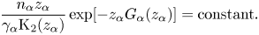
When considering the non-relativistic limit, (2.3) produces the typical outcome for a monoatomic ideal gas ($n_{\alpha }/\gamma _{\alpha }T^{3/2}_{\alpha }= \text {constant}$ ). On the other hand, when examining the ultrarelativistic limit, the equation of state for the photon gas is obtained ($n_{\alpha }/\gamma _{\alpha }T^{3}_{\alpha }= \text {constant}$
 ).
).
In order to express model equations in dimensionless form, we will use the electron skin depth ($\lambda _{e}=\sqrt {m_{0}c^{2}/8{\rm \pi} n_{0}e^{2}}$ , where $n_{0}$
 is plasma species density in the rest frame), Alfvén speed ($v_{A}=B_{0}/(8{\rm \pi} m_{0}n_{0})^{1/2}$
 ), some arbitrary magnetic field $B_{0}$
 , and $\lambda _{e}/v_{A}$
 to normalize length, plasma species velocities, magnetic field and time, respectively. Now, from (2.2) along with relations $\boldsymbol {E}=-\boldsymbol {\nabla }\phi -c^{-1}\partial \boldsymbol {A}/\partial t$
 and $\boldsymbol {B}=\boldsymbol {\nabla }\times \boldsymbol {A}$
 , the normalized equations of motion for electron and positron species are
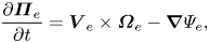
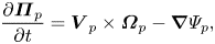
where $\boldsymbol {\varPi }_{e,p}=G\boldsymbol {V}_{e}\mp \boldsymbol {A}$ , $\boldsymbol {\varOmega }_{e,p}=\boldsymbol {\nabla }\times G\boldsymbol {V}_{e}\mp \boldsymbol {B}$
 , $\varPsi _{e,p}=c^{2}_{A}G\pm \phi$
 , $c_{A}=c/v_{A}$
 and $\phi$
 is scalar electric potential. In the above equations $\boldsymbol {\varPi _{\alpha }}$
 is generalized or canonical momentum while $\boldsymbol {\varOmega _{\alpha }}$
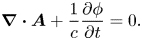
 is generalized or canonical vorticity of plasma species. In order to incorporate the effect of photon mass and couple the independent dynamics of plasma species, we employ Ampere's law, as expressed in (1.3), while assuming that displacement currents can be neglected due to the non-relativistic directed flow velocities ($\gamma _{e,p}\approx 1$
 ) of the plasma species. In normalized form, it can be expressed as
As mentioned earlier, $\lambda _{p}=h/m_{\nu }c$ , and in this study we will use $m_{\nu }\leq 10^{-49}$
 g and corresponding to this value, $\lambda _{p}\geq 1$
 au (Adelberger et al. Reference Adelberger, Dvali and Gruzinov2007). It is important to note that in massive electromagnetism, $\boldsymbol {A}$
 and $\phi$
 are observable quantities that effect the dynamics of plasma and also satisfy the following Lorentz condition:
We can now obtain the vortex evolution equations for plasma species by taking the curl of the equations of motion ((2.4)–(2.5))
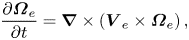
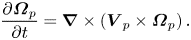
From (2.8)–(2.9), it is also evident that there is no role for gradient terms in vortex evolution. The steady-state solution of the vortex dynamics equations gives the following two equations:


where $a$ and $b$
 are called Beltrami parameters. It is also essential to highlight that (2.10)–(2.11) are also steady-state solutions of equations of motion (2.4)–(2.5) provided the gradient terms vanish independently ($\boldsymbol {\nabla }\varPsi _{e,p}=0$
 ). The condition $\boldsymbol {\nabla }\varPsi _{e,p}=0$
 , provides Bernoulli's condition ($\varPsi _{e,p}=\text {constant}$
 ), whereas the condition, in which generalized vorticities are aligned with flows ($\boldsymbol {\varOmega _{\alpha }}\parallel \boldsymbol {V_{\alpha }}$
 ), is known as the Beltrami condition. The equilibrium state described by these Beltrami and Bernoulli conditions is referred to as the Beltrami–Bernoulli equilibrium state. So the Beltrami–Bernoulli conditions ($\boldsymbol {\varOmega _{\alpha }}\parallel \boldsymbol {V_{\alpha }}$
 and $\varPsi _{e,p}=\text {constant}$
 ), in conjunction with Ampere's law, equation of state (2.3) and continuity equation (2.1), constitute a comprehensive equilibrium system that can be used to determine fields and flows. It is also worth noting that for steady-state (i.e. for constant density) continuity equations ($n_{\alpha } \boldsymbol {\nabla }\boldsymbol {\cdot }\boldsymbol {{V}_{\alpha }}=0$
 ) for plasma species, the incompressibility conditions for magnetic field and flow are inherently satisfied by the Beltrami conditions (Berezhiani, Shatashvili & Mahajan Reference Berezhiani, Shatashvili and Mahajan2015) which also lead to conservation of generalized vorticities of plasma species ($\boldsymbol {\nabla }\boldsymbol {\cdot }\boldsymbol {{\varOmega }_{\alpha }}=0$
 ). Moreover, the Beltrami parameters ($a$
 and $b$
 ) in (2.10)–(2.11) are linked with generalized helicities of plasma species, which are the ideal invariants of this plasma system. The equations of motion ((2.4)–(2.5)), Ampere's law (2.6) and vortex dynamics ((2.8)–(2.9)) yield three ideal invariants or constants of motion for this plasma model (Steinhauer & Ishida Reference Steinhauer and Ishida1997; Mahajan & Lingam Reference Mahajan and Lingam2015), namely the generalized helicity of electron ($h_{e}$
 ) and positron ($h_{p}$
 ) species and magnetofluid energy ($W$
 ) that can be expressed as
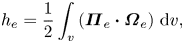
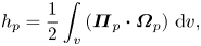
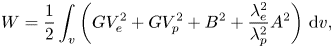
where $\int _{v}$ is a volume integral and $dv$
 is a volume element. It is also essential to note that the overall volumetric magnetic energy density in Proca electrodynamics exhibits a comparable characteristic to that of Maxwellian electrodynamics. Nevertheless, a deviation from the Maxwellian characteristic can be observed in the overall magnetic pressure within the framework of Proca electrodynamics. This deviation arises due to the negative contribution of the massive photon ($\lambda _{e}^{2}A^{2}/\lambda _{p}^{2}$
 ) to this particular quantity. Consequently, the plasma dynamics can undergo significant modifications due to the presence of negative Proca pressure, which exerts a force that pulls plasmas towards regions with higher magnetic field strength (Ryutov et al. Reference Ryutov, Budker and Flambaum2019; Bhattacharjee Reference Bhattacharjee2023). In this study, we will focus only on Beltrami conditions ((2.10)–(2.11)) to derive an equilibrium state. But it is important to mention here that the variational technique is another approach to derive a relaxed state equation, in which the ideal invariants of the plasma system are minimized. Now, the functional to be minimized in order to obtain an equilibrium state can be written as
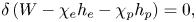
where $\chi _{e}$ and $\chi _{p}$
 are some arbitrary and real-valued constants. In the calculus of variation, these constants are called Lagrange multipliers. Upon setting the independent variations of $\delta \boldsymbol {V}_{e}$
 , $\delta \boldsymbol {V}_{p}$
 and $\delta \boldsymbol {A}$
 equal to zero, a set of three equations ((2.6) and (2.10)–(2.11)) can also be retrieved.
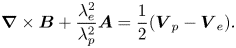
Now, in order to derive an equation describing the relaxed state, we will simultaneously solve (2.6) and (2.10)–(2.11). From (2.6), substituting the value of $\boldsymbol {V}_{e}$ in (2.10), we get

where $( \boldsymbol {\nabla }\times ) ^{3}=\boldsymbol {\nabla }\times \boldsymbol {\nabla }\times \boldsymbol {\nabla }\times$ and $( \boldsymbol {\nabla } \times ) ^{2}=\boldsymbol {\nabla }\times \boldsymbol {\nabla }\times$
 . The expression for $\boldsymbol {V}_{p}$
 can be obtained by substituting the value of $\boldsymbol {V}_{e}$
 from (2.16) into (2.6), and it is given by

Also, the bulk fluid velocity $\boldsymbol {V}$ (where $\boldsymbol {V}=0.5[\boldsymbol {V}_{e} +\boldsymbol {V}_{p}]$
 ) of plasma by using the values $\boldsymbol {V}_{e}$
 and $\boldsymbol {V}_{p}$
 from (2.16)–(2.17) in terms of $\boldsymbol {A}$
 , can be expressed as

where $d_{1}=2/( b-a)$ , $d_{2}=0.5d_{1}( a+b)$
 , $d_{3}=d_{1}(G^{-1}+\lambda _{e}^{2}\lambda _{p}^{-2})$
 and $d_{4}=0.5d_{1}\lambda _{e}^{2}\lambda _{p}^{-2}( a+b)$
 . It is also important to note that (2.16)–(2.18) demonstrate a clear indication of a robust coupling between the field and flow in the relaxed state. The equation for the relaxed state, expressed in terms of $\boldsymbol {A}$
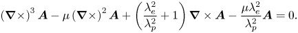
 , can be derived by replacing the value of $\boldsymbol {V}_{e}$
 from (2.16) into (2.10), and it is given by

where $( \boldsymbol {\nabla }\times ) ^{4}=\boldsymbol {\nabla }\times \boldsymbol {\nabla }\times \boldsymbol {\nabla }\times \boldsymbol {\nabla }\times$ , $k_{1}=a+b$
 , $k_{2}=ab+G^{-1}+\lambda _{e}^{2}\lambda _{p}^{-2}$
 , $k_{3}=(a+b) (0.5G^{-1}+\lambda _{e}^{2}\lambda _{p}^{-2})$
 and $k_{4}=ab\lambda _{e}^{2}\lambda _{p}^{-2}$
 . The relaxed state of a relativistic hot pair plasma with non-zero photon mass, which is described by (2.19) in terms of $\boldsymbol {A}$
 , is referred to as the QB state. The emergence of a QB state in this system can be attributed to the incorporation of inertia of electron and positron species with distinct generalized helicities of electrons and positrons (i.e. distinct Beltrami parameters $a$
 and $b$
 ) and non-zero mass of mobile fluid photons. The theoretical framework of vortical dynamics considers the interaction between the magnetic field, flow and massive photon field as being of equal importance. In this framework, the photon is conceptualized as a mobile fluid within the system. It is important to highlight that in Maxwellian electrodynamics, a photon has the potential to acquire an effective mass while it undergoes propagation within a plasma medium. Therefore, the formalism presented in this paper is based on the fundamental assumption that photons are a mobile fluid with a non-zero rest mass and that their dynamics can be derived from the Proca Lagrangian (Anderson Reference Anderson1963; Mendonça, Martins & Guerreiro Reference Mendonça, Martins and Guerreiro2000; Bhattacharjee Reference Bhattacharjee2023).
Additionally, by neglecting the mass of photons, the TB state, which has been the subject of investigation by Iqbal et al. (Reference Iqbal, Berezhiani and Yoshida2008), can be derived. On the other hand, from the Beltrami conditions and Ampere's law, as described by (2.6) and (2.10)–(2.11), with the following assumptions: $a=b=\mu$ and $G=1$
 , the resulting relaxed state equation is a TB state that is given by
So from TB equation (2.20) it is evident that when the same generalized helicities are used for both plasma species and non-relativistic regimes, the relaxed state of this plasma model seems to be the same as what Bhattacharjee (Reference Bhattacharjee2023) found for non-relativistic single species quasineutral incompressible plasma.
3 General properties of the QB state
The QB state (2.19) can be expressed as the linear superposition of four distinct force-free Beltrami states and is characterized by four scale parameters ($\lambda _{j}$ ). These scale parameters are measures of shear or twist ($\lambda =\boldsymbol {J}\boldsymbol {\cdot }\boldsymbol {B}/B^{2}$
 ), while the inverse of them gives the size (dimensionally $\lambda _{j}$
 is equal to inverse of the length) of the relaxed state structures. Here, the commutative property of the curl operator allows us to write the QB equation (2.19) in terms of scale parameters in the following manner:

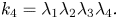
From (3.1), the scale parameters ($\lambda _{j}$ ) can be related to the coefficients $k_{j}$
 of the QB equation (2.19) in the following way:


These relations between $\lambda _{j}$ and $k_{j}$
 also satisfy Vieta's formula, so the values of scale parameters are the roots of the following quartic equation:

The formulae for calculating the eigenvalues ($\lambda _{j}$ ) of the QB state from the quartic equation (3.6) are as follows:

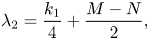
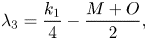
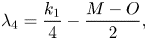
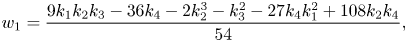
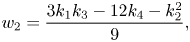
where the values of $M$ , $N$
, $N$ and $O$
 are given by
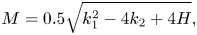

whereas in the case of $M\neq 0$ , $N$
, $N$ and $O$
 are given by


but when $M=0$ ,
,
Equations (3.7)–(3.10) demonstrate that the eigenvalues are dependent on the plasma parameters, specifically the electron skin depth, Compton wavelength of photon, Beltrami parameters and relativistic temperatures of plasma species. The eigenvalues associated with this QB state are either real or a combination of two real and a pair of complex conjugate eigenvalues. One simple approach for conducting an analysis of the characteristics of scale parameters requires employing the discriminant ($D$ ) of the quartic equation (3.6). For example, when $D<0$
 , two scale parameters are real and the other two are complex conjugate to each other. On the other hand, when $D>0$
 , all of the scale parameters are either real or complex conjugate. More specifically, all the eigenvalues are real and distinct when $D>0$
 , $S=16k_{1}^{2}k_{2}-3k_{1}^{4}-16k_{1}k_{3}-16k_{2}^{2}+64k_{4}<0$
 and $T=8k_{2}-3k_{1}^{2}<0$
 , but when $D$
 , $S$
, $S$ and $T$
 are greater than zero, there are two pairs of complex conjugate eigenvalues.
To see a glimpse of the character of scale parameters, the conditions $D>0$ , $S<0$
 and $T<0$
 , have been plotted in figure 1 as a function of Beltrami parameters and thermal energy. In the coloured region, all the scale parameters are real, while in the transparent region, two scale parameters are complex conjugate to each other and the other two are real and distinct. Figure 1 demonstrates that for Alfvénic or super-Alfvénic flows of plasma species at lower relativistic temperatures, two scale parameters are real while the other two are complex conjugates. It is important to mention that the Beltrami parameters are basically the ratio between the flow vorticity modified magnetic field and the respective flow of plasma species ($\lvert \boldsymbol {B}\pm \boldsymbol {\nabla }\times G\boldsymbol {V_{\alpha }}\rvert /\lvert G\boldsymbol {V_{\alpha }\rvert }$
 ). So when $a,b\leq 1$
 , the flow is Alfvénic or super-Alfvénic, but when $a,b>1$
 the flow is sub-Alfvénic. Now, it can be seen from the plot when the flows become sub-Alfvénic and the relativistic temperature of plasma species increases, some of the complex eigenvalues become real. So from the plot, it can be concluded that at higher relativistic temperatures and for sub-Alfvénic flows, scale parameters are real and distinct. Corresponding to these real eigenvalues, the relaxed state shows a paramagnetic trend, whereas for the combination of real and complex eigenvalues, the plasma shows diamagnetic or partial diamagnetic behaviour.

Figure 1. Nature of the eigenvalues of the QB state as a function of $a$ , $b$
, $b$ and $G$
 . In the coloured region all the eigenvalues are real and distinct.
Furthermore, in figure 2, we demonstrate the effect of relativistic temperature on the nature and variation in the sizes of scale parameters for fixed values of Beltrami parameters ($a=1.0$ and $b=2.0$
 ) by plotting $\lambda _{j}$
 from (3.7)–(3.10). From the plot, it can be seen that when the plasma is non-relativistic, i.e. $G=1$
 , there are only two real eigenvalues, while the other two are complex. The values of scale parameters are $\lambda _{1}=2.08\times 10^{-12}$
 , $\lambda _{2,3}=0.6032\pm 0.6874i$
 and $\lambda _{4}=1.794$
 . By increasing the relativistic temperature to $G=2.65$
 , all the eigenvalues become real and have the following values: $\lambda _{1}=5.521\times 10^{-12}$
 , $\lambda _{2}=0.5268$
 , $\lambda _{3}=0.5622$
 , and $\lambda _{4}=1.9109$
 . In the case of an ultrarelativistic regime, for instance, when $G=8.0$
 , the eigenvalues have the following values: $\lambda _{1}=1.67\times 10^{-11}$
 , $\lambda _{2}=0.1026$
 , $\lambda _{3}=0.9281$
 and $\lambda _{4}=1.9693$
 . From figure 2 and the values of scale parameters for different relativistic temperatures, it is very clear that by increasing the relativistic temperature, all the scale parameters become real and distinct, and the values of scale parameters $\lambda _{1}$
 , $\lambda _{3}$
 and $\lambda _{4}$
 increase while the value of $\lambda _{2}$
 decreases. Also, the eigenvalues show scale separation, which provides the possibility of multiscale structure formation.

Figure 2. Character and variation in the sizes of the scale parameters as a function of thermal energy $G$ for $a=1.0$
 and $b=2.0$
 .
.
4 Analytical solution of the QB state
As the QB field is a linear superposition of four distinct single Beltrami fields, so the analytical solution can be expressed as
where $C_{\alpha }$ are constants that can be calculated using appropriate boundary conditions and $\boldsymbol {F}_{\alpha }$
 is the Beltrami field satisfying the following conditions:
where $\lambda _{\alpha }$ is a constant number either real or complex valued, $\varGamma$
 ($\subset R^{3}$
 ) is a bounded domain with a smooth boundary $\partial \varGamma$
 , and $\boldsymbol {n}$
 is the unit normal vector onto $\partial \varGamma$
 . Note that two important examples of Beltrami fields are the Chandrasekhar–Kendall functions in cylindrical geometry and Arnold–Beltrami–Childress fields in slab geometry (Chandrasekhar & Kendall Reference Chandrasekhar and Kendall1957; Moffatt Reference Moffatt1978). Here, in an axisymmetric cylindrical geometry, the Beltrami field $\boldsymbol {F}_{\alpha }$
 can be given as
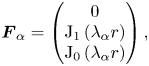
where ${\rm J}_{0}$ and ${\rm J}_{1}$
 are Bessel functions of first kind. Now, we use the following boundary conditions to calculate the values of $C_{\alpha }$
 : $\vert \boldsymbol {A}_{z}\vert _{r=0}=b_{1}$
 , $\vert \boldsymbol {A}_{\theta }\vert _{r=d} =b_{2}$
 , $\vert ( \boldsymbol {\nabla }\times \boldsymbol {A}) _{z}\vert _{r=0}=b_{3}$
 and $\vert ( \boldsymbol { \nabla }\times \boldsymbol {A}) _{\theta }\vert _{r=d}=b_{4}$
 , where $b_{\alpha }$
 and $d$
 are some real valued arbitrary constants. From these boundary conditions, $C_{\alpha }=R_{\alpha }L^{-1}$
 , where


where $\varLambda _{1}=\lambda _{1}-\lambda _{2}$ , $\varLambda _{2}=\lambda _{1}-\lambda _{3}$
 , $\varLambda _{3}=\lambda _{1}-\lambda _{4}$
 , $\varLambda _{4}=\lambda _{2}-\lambda _{3}$
 , $\varLambda _{5}=\lambda _{2}-\lambda _{4}$
 , $\varLambda _{6}=\lambda _{3}-\lambda _{4}$
 , $\varLambda _{7}=b_{4}-b_{2}\lambda _{3}$
 , $\varLambda _{8}=b_{3}-b_{1}\lambda _{4}$
 , $\varLambda _{9}=b_{3}-b_{1}\lambda _{2}$
 , $\varLambda _{10}=b_{1}\lambda _{3}-b_{3}$
 , $\varLambda _{11}=b_{4}-b_{2}\lambda _{2}$
 , $\varLambda _{12}=b_{3}-b_{1}\lambda _{1}$
 and $\varLambda _{13}=b_{2}\lambda _{1}-b_{4}$
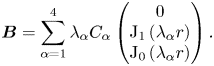
 . Now by applying the relation $\boldsymbol {B}=\boldsymbol {\nabla }\times \boldsymbol {A}$
 , the following expression can be obtained for the magnetic field:
Similarly, from the (2.18), the analytical solution for composite flow $\boldsymbol {V}$ can be written as
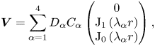
where $D_{\alpha }=d_{1}\lambda _{\alpha }^{3}-d_{2}\lambda _{\alpha }^{2}+d_{3}\lambda _{\alpha }-d_{4}$ . After formulating the analytical solution for the magnetic field and flow, we will now focus on the effect of the thermal energy of plasma species for the fixed values of Beltrami parameters on the relaxed state and also on the formation of multiscale structures and their implications. As stated in the introduction, relativistic hot EP can exist in numerous astrophysical environments, including the early universe, pulsar magnetospheres and AGN. But in this study, we will work with a low-density plasma with $n=1\,{\rm cm}^{-3}$
 (for which $\lambda _{e}$
 is $3.75\times 10^{5}\,{\rm cm}$
 ) (Iqbal et al. Reference Iqbal, Berezhiani and Yoshida2008) to model large-scale structures with arbitrary values of Beltrami parameters and relativistic temperatures. In figure 3, for the given values of plasma parameters, i.e. $a=1.0, b=2.0, b_{1}=0.8, b_{2}=2.0, b_{3}=1.0$
 and $b_{4}=0.1$
 , the effect of thermal energy $G$
 on the variations of the magnetic structures is illustrated. For the aforementioned plasma parameters when $G = 2$
 , two eigenvalues are real while the other two are complex conjugate ($\lambda _{1}=4.17\times 10^{-18}$
 , $\lambda _{2}=1.89$
 and $\lambda _{3,4}=0.558\pm 0.295i$
 ). For this combination of real and complex eigenvalues, the relaxed state shows a diamagnetic trend. On the other hand, for an ultrarelativistic regime, such that when $G = 8$
 , all the eigenvalues become real, and their values are $\lambda _{1}=1.67\times 10^{-17}$
 , $\lambda _{2}=0.103$
 , $\lambda _{3}=0.93$
 and $\lambda _{4}=1.97$
 . Corresponding to these real-valued scale parameters, the magnetic field shows a paramagnetic trend. It is abundantly clear from this analysis that for the given Beltrami parameters with appropriate boundary conditions, the thermal energy of plasma species can transform the behaviour of relaxed state structures.
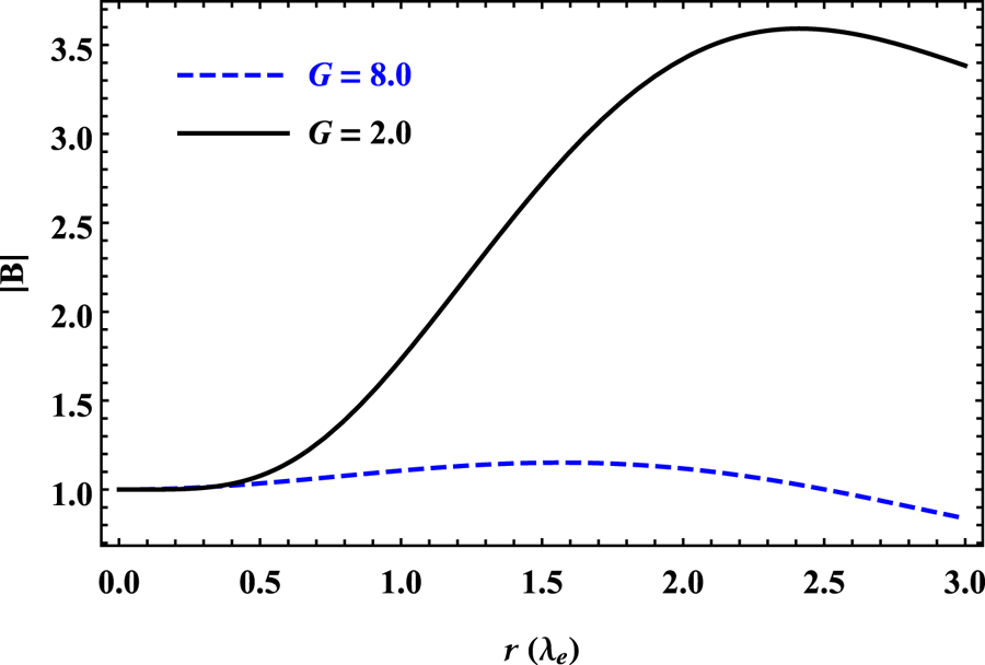
Figure 3. Profiles of QB magnetic field for $a=1.0$ , $b=2.0$
 , $G=2.0$
 (solid) and $8.0$
 (dashed).
In the subsequent discussion, we will demonstrate that the formation of multiscale structures in this QB state can create microscale kinetic or magnetic energy reservoirs. Consider the scenario when $a\approx b \gg G$ , in which the values of plasma parameters are $a=40.0, b=39.7$
 and $G=8.0$
 . From these plasma parameters, one can obtain the following values of the scale parameters: $\lambda _{1}=4.98\times 10^{-10}$
 , $\lambda _{2}=0.003$
 , $\lambda _{3}=39.7$
 and $\lambda _{4}=39.99$
 . As mentioned earlier that for a photon of mass $10^{-49}$
 g the value of $\lambda _{p}$
 is $3\times 10^{11}\,{\rm cm}$
 (Adelberger et al. Reference Adelberger, Dvali and Gruzinov2007; Particle Data Group 2022) whereas for a plasma with a number density of $n=1\,{\rm cm}^{-3}$
 , $\lambda _{e}$
 is $3.75\times 10^{5}\,{\rm cm}$
 , so the sizes of relaxed state vortices corresponding to the scale parameters are $l_{1}=7.53\times 10^{14}\,{\rm cm}$
 , $l_{2}=1.19\times 10^{8}\,{\rm cm}$
 , $l_{3}=9.45\times 10^{3}\,{\rm cm}$
 and $l_{4}=9.37\times 10^{3}\,{\rm cm}$
 . From these dimensions of the vortices, the existence of multiscale structures ($l_{1}\gg \lambda _{p}$
 , $l_{2}\gg \lambda _{e}$
 and $l_{3,4}\ll \lambda _{e}$
 ) in the QB state is evident. Next, we investigate the effect of these multiscale structures on the field and flow profiles for some suitable boundary conditions ($b_{1}=0.2$
 , $b_{2}=1.0$
 , $b_{3}=0.1$
 and $b_{4}=0.3$
 ). Figure 4 shows that the magnetic field is weak and jittery while the flow is smooth and strong. From the plot, one can also infer that the relatively small value of the magnetic field is created by the conversion of kinetic energy into magnetic energy. During this process of converting one kind of energy into another, the flow field is acting in opposition to the Lorentz force. Therefore, the presence of two microscale structures and two macroscale structures in the QB equilibrium state indicates that ambient kinetic energy dominates over magnetic energy.
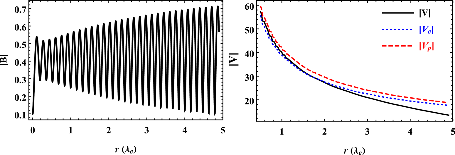
Figure 4. Magnetic field and flow profiles for $a=40.0$ , $b=39.7$
 and $G=8.0$
 .
.
Consider another case when $a\gg b$ with following values of plasma parameters and boundary conditions: $a=20.0$
 , $b=1.0$
 , $G=8.0$
 , $b_{1}=2.0$
 , $b_{2}=4.0$
 , $b_{3}=0.11$
 and $b_{4}=0.075$
 . The eigenvalues of the relaxed state for these plasma parameters are $\lambda _{1}=2.38\times 10^{-11}$
 , $\lambda _{2}=0.07$
 , $\lambda _{3}\approx b$
 and $\lambda _{4}\approx a$
 . Corresponding to these eigenvalues, the lengths of equilibrium state vortices are $l_{1}=1.57\times 10^{16}\,{\rm cm}$
 , $l_{2}=5.33\times 10^{6}\,{\rm cm}$
 , $l_{3}=4.02\times 10^{5}\,{\rm cm}$
 and $l_{4}=1.87\times 10^{4}\,{\rm cm}$
 . The scale hierarchy of these structures is $l_{1}\gg \lambda _{p}$
 , $l_{2}>\lambda _{e}$
 , $l_{3}\sim \lambda _{e}$
 , and $l_{4}<\lambda _{e}$
 . Corresponding to these multiscale structures, figure 5 illustrates that the magnetic field is strong and smooth, whereas the flow is weak and jittery. Moreover, this trend also indicates that ambient magnetic energy is higher than kinetic energy.
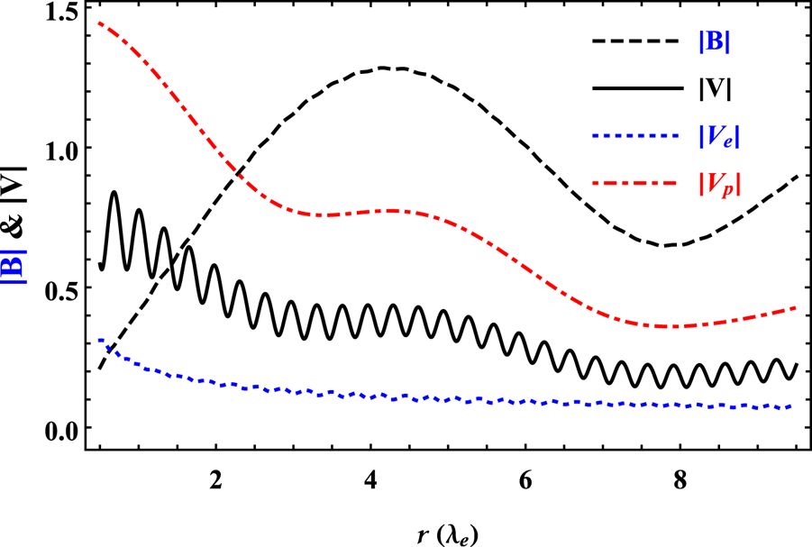
Figure 5. Magnetic field and flow profiles for $a=20.0$ , $b=1.0$
 and $G=8.0$
 .
.
The role of these ambient microscale energy reservoirs in relaxed states in driving dynamo and reverse dynamo mechanisms in astrophysical plasmas has been investigated by many authors (Mininni et al. Reference Mininni, Gómez and Mahajan2002; Mahajan et al. Reference Mahajan, Shatashvili, Mikeladze and Sigua2005; Lingam & Mahajan Reference Lingam and Mahajan2015; Kotorashvili et al. Reference Kotorashvili, Revazashvili and Shatashvili2020; Kotorashvili & Shatashvili Reference Kotorashvili and Shatashvili2022). In the dynamo process, magnetic fields are generated by the motion of an electrically conducting fluid. This phenomenon is characterized by the conversion of kinetic energy into magnetic energy. On the other hand, the reverse dynamo process involves the transformation of magnetic energy into kinetic energy and the generation of flow from the magnetic field. Therefore, based on the aforementioned discussion and the values of scale parameters calculated based on the plasma parameters and photon mass, several potential implications of the current investigation can be realized. For instance, in astrophysical EP plasmas, any observational signatures of magnetic field structures larger than the Compton wavelength can be used to set an upper limit on photon mass (Ryutov Reference Ryutov2007, Reference Ryutov2010; Bhattacharjee Reference Bhattacharjee2023). Moreover, the hypothetical Maxwell–Proca stress resulting from a non-zero photon mass in the relaxed state may play a role in the comprehension of flat galactic rotation curves (Ryutov et al. Reference Ryutov, Budker and Flambaum2019) as well as pulsar spin-down. For instance, in a recent study, Yang & Zhang (Reference Yang and Zhang2017) devised a new method for establishing a photon mass limit by exploiting spin-down information from pulsars. In the case of AGNs, it is also possible to hypothesize that if the galactic rotation curves are flat, this could indicate that AGNs can accrete gas from a greater volume of space. This may enable them to grow faster and become more powerful. The flatness of the curves may aid in channelling gas into the central regions of galaxies, where it may fuel the development of a supermassive black hole. Moreover, in plasmas, the microscale field and flow structures serve as energy reservoirs for driving dynamo and reverse dynamo mechanisms (Mahajan et al. Reference Mahajan, Shatashvili, Mikeladze and Sigua2005). But in the context of Maxwell–Proca electrodynamics, these kinds of studies have not been done yet. As the QB state has both large-scale and small-scale structures, the dynamo and reverse dynamo mechanisms, employing the standard methodology developed by Mahajan et al. (Reference Mahajan, Shatashvili, Mikeladze and Sigua2005), can also be used in the framework of Maxwell–Proca electrodynamics in future studies.
5 Summary
The relaxed state of relativistic hot EP plasma has been investigated for the very first time by incorporating the effect of non-zero photon mass. In this study, Maxwell–Proca electrodynamics has been utilized to account for the effects of non-zero photon mass. From relativistic macroscopic evolution equations for inertial hot pair species and a modified Ampere's law that also accounts for the inertial effect of photons, a QB relaxed state for the magnetic vector potential has been derived. The QB state is a non-force-free state that is a linear sum of four single force-free fields and is characterized by four self-organized vortices, which also show significant field and flow coupling. This QB equilibrium state can also be derived by the constrained minimization of ideal invariants of the plasma system. Based on the above-mentioned model equations, the ideal invariants of this plasma system are the generalized helicities for pair species and the magnetofluid energy. The expression for magnetofluid energy also demonstrates that due to the incorporation of the inertia of mobile fluid photons, there is a negative Maxwell–Proca stress that can pull plasmas towards a stronger magnetic field. Furthermore, the analysis of the relaxed state shows that at higher relativistic temperatures and for larger values of Beltrami parameters, all the scale parameters become real and distinct. The QB self-organized vortices also show a multiscale nature, and the inclusion of non-zero photon mass in the plasma model guarantees the existence of one self-organized structure larger than the Compton wavelength of the photons. However, any observational signatures connected to these multiscale structures can also serve as a crucial basis for refining the estimates of the upper bound on the photon mass. Additionally, the analytical solution for magnetic field and coupled plasma flow for this QB state in an axisymmetric cylindrical geometry is provided. The analysis of the field profiles shows that at lower relativistic temperatures, plasma has a diamagnetic trend for certain values of Beltrami parameters. Also, the formation of multiscale structures can create microscale reservoirs of kinetic or magnetic energy. This ambient microscale kinetic or magnetic energy has the potential to significantly contribute to the creation of macroscopic fields and flows through dynamo and reverse dynamo processes. In conclusion, the presence of QB multiscale self-organized field structures in relativistic pair plasma, within the framework of Proca electrodynamics, has the potential to contribute to the resolution of challenges such as the upper limit on photon mass and galactic rotation curves.
Acknowledgements
Editor D. Uzdensky thanks the referees for their advice in evaluating this article.
Funding
The work of M.I. is supported by Higher Education Commission (HEC), Pakistan, under project no. 20-9408/Punjab/NRPU/R&D/HEC/2017-18.
Declaration of interests
The authors report no conflict of interest.


 Open access