


1 Introduction
Let X be a Cohen–Macaulay scheme of pure dimension and
 $\mathscr {G}$
a coherent sheaf on X of rank r and homological dimension
$\mathscr {G}$
a coherent sheaf on X of rank r and homological dimension
 $\le 1$
– that is, locally over X, there is a two-step resolution
$\le 1$
– that is, locally over X, there is a two-step resolution
 $0 \to \mathscr {F} \to \mathscr {E} \to \mathscr {G} \to 0$
, where
$0 \to \mathscr {F} \to \mathscr {E} \to \mathscr {G} \to 0$
, where
 $\mathscr {F}$
and
$\mathscr {F}$
and
 $\mathscr {E}$
are finite locally free sheaves. (If X is regular, this condition on
$\mathscr {E}$
are finite locally free sheaves. (If X is regular, this condition on
 $\mathscr {G}$
is equivalent to
$\mathscr {G}$
is equivalent to
 $\mathscr {E} \kern -1pt xt^i_X(\mathscr {G},\mathscr {O}_X) =0$
for all
$\mathscr {E} \kern -1pt xt^i_X(\mathscr {G},\mathscr {O}_X) =0$
for all
 $i \ge 2$
.) The projectivization
$i \ge 2$
.) The projectivization
 $\pi \colon \mathbb {P}(\mathscr {G}) : = \operatorname {Proj}_X \operatorname {Sym}_{\mathscr {O}_X}^\bullet \mathscr {G} \to X$
of
$\pi \colon \mathbb {P}(\mathscr {G}) : = \operatorname {Proj}_X \operatorname {Sym}_{\mathscr {O}_X}^\bullet \mathscr {G} \to X$
of
 $\mathscr {G}$
is generically a projective bundle with fiber
$\mathscr {G}$
is generically a projective bundle with fiber
 $\mathbb {P}^{r-1}$
; however, the dimension of the fiber of
$\mathbb {P}^{r-1}$
; however, the dimension of the fiber of
 $\pi $
jumps along the degeneracy loci (see §2.1) of
$\pi $
jumps along the degeneracy loci (see §2.1) of
 $\mathscr {G}$
.
$\mathscr {G}$
.
The derived category of
 $\mathbb {P}(\mathscr {G})$
was studied in [Reference Jiang, Leung and Xie25], where we proved (under certain regularity and dimension conditions) that there is a semiorthogonal decomposition
$\mathbb {P}(\mathscr {G})$
was studied in [Reference Jiang, Leung and Xie25], where we proved (under certain regularity and dimension conditions) that there is a semiorthogonal decomposition
 $$ \begin{align*} \mathrm{D^b_{coh}}(\mathbb{P}(\mathscr{G})) = \left \langle \mathrm{D^b_{coh}}\left(\mathbb{P}\left(\mathscr{E} \kern -1pt xt^1(\mathscr{G},\mathscr{O}_X)\right)\right),\ \mathrm{D^b_{coh}}(X)\otimes \mathscr{O}(1), \dotsc, \mathrm{D^b_{coh}}(X)\otimes \mathscr{O}(r)\right \rangle. \end{align*} $$
(For a space Y,
 $\mathrm {D^b_{coh}}(Y)$
stands for its bounded derived category of coherent sheaves.) The theorem states that the (right) orthogonal of the ‘projective bundle part’ of
$\mathrm {D^b_{coh}}(Y)$
stands for its bounded derived category of coherent sheaves.) The theorem states that the (right) orthogonal of the ‘projective bundle part’ of
 $\mathrm {D^b_{coh}}(\mathbb {P}(\mathscr {G}))$
is given by the derived category of another projectivization
$\mathrm {D^b_{coh}}(\mathbb {P}(\mathscr {G}))$
is given by the derived category of another projectivization
 $\mathbb {P}\left (\mathscr {E} \kern -1pt xt^1(\mathscr {G},\mathscr {O}_X)\right )$
, which is a Springer-type partial desingularization of the singular locus of
$\mathbb {P}\left (\mathscr {E} \kern -1pt xt^1(\mathscr {G},\mathscr {O}_X)\right )$
, which is a Springer-type partial desingularization of the singular locus of
 $\mathscr {G}$
(see [Reference Jiang, Leung and Xie25] for more details).
$\mathscr {G}$
(see [Reference Jiang, Leung and Xie25] for more details).
In this paper, we establish the Chow-theoretic version of this formula:
Theorem see Theorem 4.1
Let X and
 $\mathscr {G}$
be as before. Assume either
$\mathscr {G}$
be as before. Assume either
-
(A)
 $\mathbb {P}(\mathscr {G})$
and
$\mathbb {P}\left (\mathscr {E} \kern -1pt xt^1(\mathscr {G},\mathscr {O}_X)\right )$
are nonsingular and quasi-projective, and the degeneracy loci of
$\mathscr {G}$
satisfy a weak dimension condition (4.1); or
$\mathbb {P}(\mathscr {G})$
and
$\mathbb {P}\left (\mathscr {E} \kern -1pt xt^1(\mathscr {G},\mathscr {O}_X)\right )$
are nonsingular and quasi-projective, and the degeneracy loci of
$\mathscr {G}$
satisfy a weak dimension condition (4.1); or -
(B) all degeneracy loci of
$\mathscr {G}$
(either are empty or) have expected dimensions.


Then for each
 $k \ge 0$
, there is an isomorphism of integral Chow groups:
$k \ge 0$
, there is an isomorphism of integral Chow groups:
 $$ \begin{align*} \operatorname{CH}_k(\mathbb{P}(\mathscr{G})) \simeq \operatorname{CH}_{k-r}\left(\mathbb{P}\left(\mathscr{E} \kern -1pt xt^1(\mathscr{G},\mathscr{O}_X)\right)\right) \oplus \bigoplus_{i=0}^{r-1} \operatorname{CH}_{k-(r-1)+i}(X). \end{align*} $$
Since the isomorphism of the theorem commutes with the product with another space, by Manin’s identity principle, if
 $\mathbb {P}(\mathscr {G})$
,
$\mathbb {P}(\mathscr {G})$
,
 $\mathbb {P}\left (\mathscr {E} \kern -1pt xt^1(\mathscr {G},\mathscr {O}_X)\right )$
and X are smooth and projective over the ground field
$\mathbb {P}\left (\mathscr {E} \kern -1pt xt^1(\mathscr {G},\mathscr {O}_X)\right )$
and X are smooth and projective over the ground field
 $\Bbbk $
, then there is an isomorphism of integral (pure effective) Chow motives:
$\Bbbk $
, then there is an isomorphism of integral (pure effective) Chow motives:
 $$ \begin{align*} \mathfrak{h}(\mathbb{P}(\mathscr{G})) \simeq \mathfrak{h}\left(\mathbb{P}\left(\mathscr{E} \kern -1pt xt^1(\mathscr{G},\mathscr{O}_X)\right)\right)(r) \oplus \bigoplus_{i=0}^{r-1} \mathfrak{h}(X)(i) \end{align*} $$
(see Corollary 4.3). Note that this result compares nicely with Vial’s work [Reference Vial52] on
 $\mathbb {P}^{r-1}$
-fibrations; in our case,
$\mathbb {P}^{r-1}$
-fibrations; in our case,
 $\mathbb {P}(\mathscr {G})$
is a generic
$\mathbb {P}(\mathscr {G})$
is a generic
 $\mathbb {P}^{r-1}$
-fibration. Taking a cohomological realization – for example, the Betti cohomology if
$\mathbb {P}^{r-1}$
-fibration. Taking a cohomological realization – for example, the Betti cohomology if
 $\Bbbk \subset \mathbb {C}$
– the isomorphism of motives induces an isomorphism of rational Hodge structures:
$\Bbbk \subset \mathbb {C}$
– the isomorphism of motives induces an isomorphism of rational Hodge structures:
 $$ \begin{align*} H^n(\mathbb{P}(\mathscr{G}), \mathbb{Q}) \simeq H^{n-2r}\left(\mathbb{P}\left(\mathscr{E} \kern -1pt xt^1(\mathscr{G},\mathscr{O}_X)\right),\ \mathbb{Q}\right) \oplus\bigoplus_{i=0}^{r-1} H^{n-2i}(X,\mathbb{Q}), \qquad \forall n \ge 0. \end{align*} $$
This paper provides two approaches to proving our theorem, one under each of the conditions (A) and (B). The idea behind both approaches is that one could view the projectivization phenomenon as a combination of the Cayley trick and flips.
We study the Chow theory for the Cayley trick in §3.1 (see Theorem 3.1 and Corollary 3.4) and the Chow theory of standard flips in §3.2 (see Theorem 3.6 and Corollary 3.10). These results are of independent interest on their own. For example, it follows from Theorem 3.1 and Corollary 3.4 that the Chow group (and., motive) of every complete intersection variety can be split-embedded into that of a Fano variety (see Example 3.5; compare [Reference Kiem, Kim, Lee and Lee28]).
The first examples of the theorem are universal
 $\operatorname {Hom}$
spaces (see §4.3.1), flops from Springer-type resolutions of determinantal hypersurfaces (see §4.3.2), and a blowup formula for blowing up along Cohen–Macaulay codimension
$\operatorname {Hom}$
spaces (see §4.3.1), flops from Springer-type resolutions of determinantal hypersurfaces (see §4.3.2), and a blowup formula for blowing up along Cohen–Macaulay codimension
 $2$
subschemes (see §4.3.3).
$2$
subschemes (see §4.3.3).
1.1 Applications
The following applications parallel the applications of the projectivization formula in the study of derived categories [Reference Jiang, Leung and Xie25].
-
(1) Symmetric powers of curves (§5.1). Let C be a smooth projective curve of genus
$g \ge 1$
and denote by
$C^{(k)}$
the kth symmetric power. For any
$0 \le n \le g-1$
, the relationships between the derived category of
$C^{(g-1+n)}$
and
$C^{(g-1-n)}$
(and also the Jacobian variety
$\operatorname {Jac}(C)$
) was established by Toda [Reference Toda51] using wall crossing of stable pair moduli, and later by [Reference del Baño5, Reference Jiang, Leung and Xie25] using the projectivization formula. The main theorem of this paper implies the corresponding Chow-theoretic version of the formula: for any
$k \ge 0$
, there is an isomorphism of integral Chow groups and a similar decomposition for integral Chow motives (see Corollary 5.1).
$$ \begin{align*} \operatorname{CH}_{k}\left(C^{(g-1+n)}\right) \simeq \operatorname{CH}_{k-n}\left(C^{(g-1-n)}\right) \oplus \bigoplus_{i=0}^{n-1} \operatorname{CH}_{k-(n-1)+i}(\operatorname{Jac}(C)), \end{align*} $$
-
(2) Nested Hilbert schemes of surfaces (§5.2). Let S be a smooth quasi-projective surface, and denote by
$\mathrm {Hilb}_{n}(S)$
the Hilbert scheme of n points on S; by convention,
$\mathrm {Hilb}_{1}(S) = S$
,
$\mathrm {Hilb}_{0} = \text {point}$
. Denote
$\mathrm {Hilb}_{n,n+1}(S)$
the nested Hilbert scheme. Then the projectivization formula of derived categories [Reference Jiang, Leung and Xie25] can be applied to obtain a semiorthogonal decomposition of
$D\left (\mathrm {Hilb}_{n,n+1}(S)\right )$
[Reference del Baño5]. In this paper we show that for any
$k \ge 0$
, there is an isomorphism of integral Chow groups and a similar decomposition for Chow motives (see Corollary 5.4).
$$ \begin{align*} \operatorname{CH}_{k}\left(\mathrm{Hilb}_{n,n+1}(S)\right) &\simeq \operatorname{CH}_{k-1}\left(\mathrm{Hilb}_{n-1,n}(S)\right) \oplus \operatorname{CH}_{k}(\mathrm{Hilb}_n(S) \times S) \\ & \simeq \bigoplus_{i=0}^n \operatorname{CH}_{k-i}(\mathrm{Hilb}_{n-i}(S) \times S), \end{align*} $$
-
(3) Voisin maps (§5.3). Let Y be a cubic fourfold not containing any plane, let
$F(Y)$
be the Fano variety of lines on Y, and let
$Z(Y)$
be the corresponding LLSvS eightfold [Reference Lehn and Lehn36]. Voisin [Reference Voisin54] constructed a rational map
$v \colon F(Y) \times F(Y) \dashrightarrow Z(Y)$
of degree
$6$
, Chen [Reference Bernardara and Tabuada9] showed that the Voisin map v can be resolved by blowing up the indeterminacy locus
$Z = \{ (L_1,L_2) \in F(Y) \times F(Y) \mid L_1 \cap L_2 \ne \emptyset \}$
, and the blowup variety is a natural relative
$Quot$
-scheme over
$Z(Y)$
if Y is very general. The main theorem can be applied to this case, and implies that for any
$k \ge 0$
, there is an isomorphism of Chow groups where
$$ \begin{align*} \operatorname{CH}_k(\operatorname{Bl}_Z ( F(Y) \times F(Y))) \simeq \operatorname{CH}_{k-1}\left(\widetilde{Z}\right) \oplus \operatorname{CH}_k(F(Y) \times F(Y)), \end{align*} $$
$\widetilde {Z} = \mathbb {P}(\omega _Z)$
is a Springer-type (partial) resolution of the indeterminacy locus Z, which is an isomorphism over
$Z \backslash \Delta _2$
, and a
$\mathbb {P}^1$
-bundle over the type II locus
$\Delta _2 = \left \{L \in \Delta \simeq F(Y) \mid \mathscr {N}_{L/Y} \simeq \mathscr {O}(1)^{\oplus 2} \oplus \mathscr {O}(-1)\right \}$
which is an algebraic surface (see Corollary 5.6).


The results of this paper could also be applied to many other situations of moduli spaces, for example, moduli of sheaves on surfaces [Reference Neguţ43, Reference Neguţ44] and the moduli spaces of extensions of stable objects in K3 categories, which are generalizations of the varieties resolving Voisin’s maps [Reference Bernardara and Tabuada9, Reference Voisin54]. Another such example is provided by the pair of Thaddeus moduli spaces [Reference Thaddeus48]
 $M_C(2,\mathscr {L}) \to N_C(2,\mathscr {L})$
and
$M_C(2,\mathscr {L}) \to N_C(2,\mathscr {L})$
and
 $M_C\left (2,\mathscr {L}^\vee \otimes \omega _C\right ) \to N_C(2,\mathscr {L})$
studied by Koseki and Toda [Reference Koseki and Toda29]. (Here,
$M_C\left (2,\mathscr {L}^\vee \otimes \omega _C\right ) \to N_C(2,\mathscr {L})$
studied by Koseki and Toda [Reference Koseki and Toda29]. (Here,
 $\mathscr {L}$
is a line bundle of odd degree
$\mathscr {L}$
is a line bundle of odd degree
 $d>0$
,
$d>0$
,
 $N_C(2,\mathscr {L})$
is the moduli space of rank
$N_C(2,\mathscr {L})$
is the moduli space of rank
 $2$
semistable vector bundles over a curve C, with determinant
$2$
semistable vector bundles over a curve C, with determinant
 $\mathscr {L}$
, and
$\mathscr {L}$
, and
 $M_C(2,\mathscr {L})$
is the space
$M_C(2,\mathscr {L})$
is the space
 $M_{\omega }$
of [Reference Thaddeus48], where
$M_{\omega }$
of [Reference Thaddeus48], where
 $\omega = \left [\frac {d-1}{2}\right ]$
). The results of this paper on flips (§3.2) and projectivizations (Theorem 4.1) would shed light on the study of the Chow theory of
$\omega = \left [\frac {d-1}{2}\right ]$
). The results of this paper on flips (§3.2) and projectivizations (Theorem 4.1) would shed light on the study of the Chow theory of
 $N_C(2,\mathscr {L})$
.Footnote
1
$N_C(2,\mathscr {L})$
.Footnote
1
1.2 Conventions
Throughout this paper, X is a Noetherian scheme of pure dimension,and
 $\mathscr {G}$
is a coherent sheaf over X. We say that
$\mathscr {G}$
is a coherent sheaf over X. We say that
 $\mathscr {G}$
has rank r if the rank of
$\mathscr {G}$
has rank r if the rank of
 $\mathscr {G}(\eta ) : = \mathscr {G} \otimes \kappa (\eta )$
is r at the generic point
$\mathscr {G}(\eta ) : = \mathscr {G} \otimes \kappa (\eta )$
is r at the generic point
 $\eta $
of each irreducible component of X. Assume that all schemes in consideration are defined over some fixed ground field
$\eta $
of each irreducible component of X. Assume that all schemes in consideration are defined over some fixed ground field
 $\Bbbk $
. The terms ‘locally free sheaves’ and ‘vector bundles’ will be used interchangeably. We use Grothendieck’s notations: for a coherent sheaf
$\Bbbk $
. The terms ‘locally free sheaves’ and ‘vector bundles’ will be used interchangeably. We use Grothendieck’s notations: for a coherent sheaf
 $\mathscr {F}$
on a scheme X, denote by
$\mathscr {F}$
on a scheme X, denote by
 $\mathbb {P}_X(\mathscr {F}) =\operatorname {Proj}_X \operatorname {Sym}_{\mathscr {O}_X}^\bullet \mathscr {F}$
its projectivization; we will write
$\mathbb {P}_X(\mathscr {F}) =\operatorname {Proj}_X \operatorname {Sym}_{\mathscr {O}_X}^\bullet \mathscr {F}$
its projectivization; we will write
 $\mathbb {P}(\mathscr {F})$
if the base scheme is clear from context. For a vector bundle V, we also use
$\mathbb {P}(\mathscr {F})$
if the base scheme is clear from context. For a vector bundle V, we also use
 $\mathbb {P}_{\mathrm {sub}}(V) : = \mathbb {P}\left (V^\vee \right )$
to denote the moduli space of
$\mathbb {P}_{\mathrm {sub}}(V) : = \mathbb {P}\left (V^\vee \right )$
to denote the moduli space of
 $1$
-dimensional linear subbundles of V.
$1$
-dimensional linear subbundles of V.
For motives, we use the covariant convention of [Reference Kahn, Murre and Pedrini27, Reference Murre41, Reference Murre42, Reference Vial52, Reference Vial53]. In particular, [Reference Kahn, Murre and Pedrini27] contains a dictionary for translating between covariant and contravariant conventions. For a smooth projective variety X over a field
 $\Bbbk $
, denote by
$\Bbbk $
, denote by
 $\mathfrak {h}(X)$
its class
$\mathfrak {h}(X)$
its class
 $(X, \operatorname {Id}_X,0)$
in Grothendieck’s category of integral Chow motives of smooth projective varieties over
$(X, \operatorname {Id}_X,0)$
in Grothendieck’s category of integral Chow motives of smooth projective varieties over
 $\Bbbk $
. Notice that under the covariant convention, for a morphism
$\Bbbk $
. Notice that under the covariant convention, for a morphism
 $f \colon X \to Y$
of smooth projective varieties,
$f \colon X \to Y$
of smooth projective varieties,
 $\Gamma _f$
induces the push-forward map
$\Gamma _f$
induces the push-forward map
 $f_* \colon \mathfrak {h}(X) \to \mathfrak {h}(Y)$
and
$f_* \colon \mathfrak {h}(X) \to \mathfrak {h}(Y)$
and
 $\left [\Gamma _f^t\right ]$
induces the pullback map
$\left [\Gamma _f^t\right ]$
induces the pullback map
 $f^* \colon \mathfrak {h}(Y) \to \mathfrak {h}(X)(\dim Y - \dim X)$
. Moreover,
$f^* \colon \mathfrak {h}(Y) \to \mathfrak {h}(X)(\dim Y - \dim X)$
. Moreover,
 $\mathfrak {h}\left (\mathbb {P}^1\right ) = 1 \oplus \mathbb {L} = 1 \oplus 1(1)$
, where
$\mathfrak {h}\left (\mathbb {P}^1\right ) = 1 \oplus \mathbb {L} = 1 \oplus 1(1)$
, where
 $1 = \mathfrak {h}(\operatorname {Spec} k)$
, and
$1 = \mathfrak {h}(\operatorname {Spec} k)$
, and
 $\mathbb {L} = 1(1)$
is the Lefschetz motive. In particular, the covariant Tate twist coincides with tensoring with
$\mathbb {L} = 1(1)$
is the Lefschetz motive. In particular, the covariant Tate twist coincides with tensoring with
 $\mathbb {L}$
– that is,
$\mathbb {L}$
– that is,
 $\mathfrak {h}(X)(i) = \mathfrak {h}(X) \otimes \mathbb {L}^i$
for all
$\mathfrak {h}(X)(i) = \mathfrak {h}(X) \otimes \mathbb {L}^i$
for all
 $i \in \mathbb {Z}$
. Furthermore,
$i \in \mathbb {Z}$
. Furthermore,
 $\operatorname {CH}^\ell (\mathfrak {h}(X)(n)) = \operatorname {CH}^{\ell - n}(X)$
and
$\operatorname {CH}^\ell (\mathfrak {h}(X)(n)) = \operatorname {CH}^{\ell - n}(X)$
and
 $\operatorname {CH}_{k}(\mathfrak {h}(X)(n)) = \operatorname {CH}_{k-n}(X)$
. We will use h to denote the action
$\operatorname {CH}_{k}(\mathfrak {h}(X)(n)) = \operatorname {CH}_{k-n}(X)$
. We will use h to denote the action
 $c_{1}(\mathscr {O}(1)) \cap (\underline {\hphantom {A}})$
on motives when the line bundle
$c_{1}(\mathscr {O}(1)) \cap (\underline {\hphantom {A}})$
on motives when the line bundle
 $\mathscr {O}(1)$
is clear from the context.
$\mathscr {O}(1)$
is clear from the context.
2 Preliminaries
2.1 Degeneracy loci
Standard references are [Reference Fulton18, Reference Fulton and Pragacz19, Reference Gelfand, Kapranov and Zelevinsky20, Reference Golubitsky and Guillemin21, Reference Lazarsfeld34].
Definition 2.1
-
(1) Let
$\mathscr {G}$
be a coherent sheaf of (generic) rank r over a scheme X. For an integer
$k \in \mathbb {Z}$
, the degeneracy locus of
$\mathscr {G}$
of rank
$\ge k$
is defined to be where
$$ \begin{align*} X^{ \ge k}(\mathscr{G}): = \{x \in X \mid \operatorname{rank} \mathscr{G}(x) \ge k\}, \end{align*} $$
$\mathscr {G}(x) := \mathscr {G}_x \otimes _{\mathscr {O}_{X,x}} \kappa (x)$
is the fiber of
$\mathscr {G}$
at
$x \in X$
. Notice that
$X^{ \ge k}(\mathscr {G}) = X$
if
$k \le r$
. We call
$X_{\mathrm {sg}}(\mathscr {G}) : = X^{\ge r+1}(\mathscr {G})$
the first degeneracy locus (or the singular locus) of
$\mathscr {G}$
.
-
(2) Let
$\sigma : \mathscr {F} \to \mathscr {E}$
be a morphism of
$\mathscr {O}_X$
-modules between locally free sheaves
$\mathscr {F}$
and
$\mathscr {E}$
on X. For an integer
$\ell $
, the degeneracy locus of
$\sigma $
of rank
$\ell $
is defined to be where
$$ \begin{align*} D_\ell(\sigma) := \{ x \in X \mid \operatorname{rank} \sigma (x) \le \ell \}, \end{align*} $$
$\sigma (x) := \sigma _x \otimes _{\mathscr {O}_{X,x}} \kappa (x) \colon \mathscr {F}(x) \to \mathscr {E}(x)$
is the map induced by
$\sigma $
on the fibers.


The degeneracy loci
 $X^{\ge k}(\mathscr {G})$
and
$X^{\ge k}(\mathscr {G})$
and
 $D_\ell (\sigma )$
have natural closed subscheme structures given by Fitting ideals [Reference Lazarsfeld34, §7,2]. The two notions are related as follows: let
$D_\ell (\sigma )$
have natural closed subscheme structures given by Fitting ideals [Reference Lazarsfeld34, §7,2]. The two notions are related as follows: let
 $\sigma \colon \mathscr {F} \to \mathscr {E}$
be an
$\sigma \colon \mathscr {F} \to \mathscr {E}$
be an
 $\mathscr {O}_X$
-module map between finite locally free sheaves and let
$\mathscr {O}_X$
-module map between finite locally free sheaves and let
 $\mathscr {G}: = \operatorname {Coker} (\sigma )$
be the cokernel. Then
$\mathscr {G}: = \operatorname {Coker} (\sigma )$
be the cokernel. Then
 $X^{\ge k}(\mathscr {G}) = D_{\operatorname {rank} \mathscr {E} - k}(\sigma )$
as closed subschemes of X.
$X^{\ge k}(\mathscr {G}) = D_{\operatorname {rank} \mathscr {E} - k}(\sigma )$
as closed subschemes of X.
The expected codimension of
 $D_{\ell }(\sigma ) \subset X$
is
$D_{\ell }(\sigma ) \subset X$
is
 $(\operatorname {rank} \mathscr {E} -\ell )(\operatorname {rank} \mathscr {F} -\ell )$
(if
$(\operatorname {rank} \mathscr {E} -\ell )(\operatorname {rank} \mathscr {F} -\ell )$
(if
 $\ell \le \min \{\operatorname {rank} \mathscr {E}, \operatorname {rank} \mathscr {F}\}$
). If
$\ell \le \min \{\operatorname {rank} \mathscr {E}, \operatorname {rank} \mathscr {F}\}$
). If
 $\mathscr {G}$
has homological dimension
$\mathscr {G}$
has homological dimension
 $\le 1$
and rank r – for example, if
$\le 1$
and rank r – for example, if
 $\mathscr {G}= \operatorname {Coker} \left (\mathscr {F} \xrightarrow {\sigma } \mathscr {E}\right )$
is the cokernel of an injective map of
$\mathscr {G}= \operatorname {Coker} \left (\mathscr {F} \xrightarrow {\sigma } \mathscr {E}\right )$
is the cokernel of an injective map of
 $\mathscr {O}_X$
-modules between finite locally free sheaves – then for any
$\mathscr {O}_X$
-modules between finite locally free sheaves – then for any
 $i \ge 0$
, the expected codimension of
$i \ge 0$
, the expected codimension of
 $X^{\ge r+i}(\mathscr {G}) \subset X$
is
$X^{\ge r+i}(\mathscr {G}) \subset X$
is
 $i(r+i)$
.
$i(r+i)$
.
In the universal local situation where
 $X=\operatorname {Hom}_\Bbbk (W,V)$
is the total space of maps between two vector spaces W and V over a field
$X=\operatorname {Hom}_\Bbbk (W,V)$
is the total space of maps between two vector spaces W and V over a field
 $\Bbbk $
, there is a tautological map
$\Bbbk $
, there is a tautological map
 $\tau \colon W \otimes \mathscr {O}_X \to V \otimes \mathscr {O}_X$
over X, such that
$\tau \colon W \otimes \mathscr {O}_X \to V \otimes \mathscr {O}_X$
over X, such that
 $\tau (A) = A$
for
$\tau (A) = A$
for
 $A \in \operatorname {Hom}(W,V)$
.
$A \in \operatorname {Hom}(W,V)$
.
Lemma 2.2. [Reference Fulton and Pragacz19, Reference Gelfand, Kapranov and Zelevinsky20, Reference Golubitsky and Guillemin21]
Let
 $X = \operatorname {Hom}_\Bbbk (W,V)$
and denote
$X = \operatorname {Hom}_\Bbbk (W,V)$
and denote
 $D_\ell = D_\ell (\tau ) \subseteq X$
the degeneracy locus of the tautological map
$D_\ell = D_\ell (\tau ) \subseteq X$
the degeneracy locus of the tautological map
 $\tau $
of
$\tau $
of
 $\operatorname {rank} \ell $
. Then for any
$\operatorname {rank} \ell $
. Then for any
 $0 \le \ell \le \min \{\operatorname {rank} W, \operatorname {rank} V\}$
, the singular locus of
$0 \le \ell \le \min \{\operatorname {rank} W, \operatorname {rank} V\}$
, the singular locus of
 $D_\ell $
is
$D_\ell $
is
 $D_{\ell -1}$
. Furthermore, for any regular point
$D_{\ell -1}$
. Furthermore, for any regular point
 $A \in D_\ell \backslash D_{\ell -1}$
, the following are true:
$A \in D_\ell \backslash D_{\ell -1}$
, the following are true:
-
(1) The tangent space of
$D_\ell $
at A is
$T_{A} D_\ell = \{T \in \operatorname {Hom}(W,V) \mid T(\operatorname {Ker} A) \subseteq \operatorname {Im} A\}$
. -
(2) The normal space of
$D_\ell $
to X at A is
$N_{D_\ell } X \rvert _{A} = \operatorname {Hom} (\operatorname {Ker} A, \operatorname {Coker} A)$
.


Proof. See [Reference Fulton and Pragacz19, §5.1, p. 54–55], [Reference Gelfand, Kapranov and Zelevinsky20, Lemma 4.12], or [Reference Golubitsky and Guillemin21, Ex. V (4), p. 145].
In general, let
 $\sigma : \mathscr {F} \to \mathscr {E}$
be a map between vector bundles over a scheme X. For a fixed integer
$\sigma : \mathscr {F} \to \mathscr {E}$
be a map between vector bundles over a scheme X. For a fixed integer
 $\ell $
, regarding the open degeneracy locus
$\ell $
, regarding the open degeneracy locus
 $D: = D_\ell (\sigma ) \backslash D_{\ell -1}(\sigma )$
we have the following:
$D: = D_\ell (\sigma ) \backslash D_{\ell -1}(\sigma )$
we have the following:
Lemma 2.3. Assume X is a Cohen–Macaulay
 $\Bbbk $
-scheme and
$\Bbbk $
-scheme and
 $D: = D_\ell (\sigma ) \backslash D_{\ell -1}(\sigma ) \subset X$
has the expected codimension
$D: = D_\ell (\sigma ) \backslash D_{\ell -1}(\sigma ) \subset X$
has the expected codimension
 $(\operatorname {rank} \mathscr {E} -\ell )(\operatorname {rank} \mathscr {F} -\ell )$
. Then
$(\operatorname {rank} \mathscr {E} -\ell )(\operatorname {rank} \mathscr {F} -\ell )$
. Then
 $\sigma \rvert _D \colon \mathscr {E}\rvert _D \to \mathscr {F}\rvert _D$
has constant rank
$\sigma \rvert _D \colon \mathscr {E}\rvert _D \to \mathscr {F}\rvert _D$
has constant rank
 $\ell $
over D, and
$\ell $
over D, and
 $K: = \operatorname {Ker} \sigma \rvert _D$
and
$K: = \operatorname {Ker} \sigma \rvert _D$
and
 $C: = \operatorname {Coker} \sigma \rvert _D$
are locally free sheaves over D of ranks
$C: = \operatorname {Coker} \sigma \rvert _D$
are locally free sheaves over D of ranks
 $\operatorname {rank} \mathscr {E} - \ell $
and
$\operatorname {rank} \mathscr {E} - \ell $
and
 $\operatorname {rank} \mathscr {F} - \ell $
, respectively. Moreover,
$\operatorname {rank} \mathscr {F} - \ell $
, respectively. Moreover,
 $D \subset X$
is a locally complete intersection subscheme with normal bundle
$D \subset X$
is a locally complete intersection subscheme with normal bundle
 $N_{D/X} \simeq K^\vee \otimes C$
.
$N_{D/X} \simeq K^\vee \otimes C$
.
Proof. First we prove the lemma for the total Hom space
 $H = \lvert \operatorname {Hom}_X(\mathscr {F},\mathscr {E})\rvert $
. Denote
$H = \lvert \operatorname {Hom}_X(\mathscr {F},\mathscr {E})\rvert $
. Denote
 $\pi \colon H = \lvert \operatorname {Hom}_X(\mathscr {F},\mathscr {E})\rvert \to X$
the projection, and let
$\pi \colon H = \lvert \operatorname {Hom}_X(\mathscr {F},\mathscr {E})\rvert \to X$
the projection, and let
 $\mathbb {D}_\ell : = D_\ell (\tau _H)\subset H$
be the degeneracy locus for the tautological map
$\mathbb {D}_\ell : = D_\ell (\tau _H)\subset H$
be the degeneracy locus for the tautological map
 $\tau _H \colon \pi ^* \mathscr {F} \to \pi ^* \mathscr {E}$
. As the statement is local, we may assume
$\tau _H \colon \pi ^* \mathscr {F} \to \pi ^* \mathscr {E}$
. As the statement is local, we may assume
 $X = \operatorname {Spec} A$
,
$X = \operatorname {Spec} A$
,
 $\mathscr {F} = W \otimes _\Bbbk A$
, and
$\mathscr {F} = W \otimes _\Bbbk A$
, and
 $\mathscr {E} = V \otimes _\Bbbk A$
, where A is a
$\mathscr {E} = V \otimes _\Bbbk A$
, where A is a
 $\Bbbk $
-algebra and
$\Bbbk $
-algebra and
 $W, V$
are
$W, V$
are
 $\Bbbk $
-vector spaces. Then
$\Bbbk $
-vector spaces. Then
 $H = \operatorname {Hom}(W, V) \times _\Bbbk X$
is the flat base change of
$H = \operatorname {Hom}(W, V) \times _\Bbbk X$
is the flat base change of
 $\operatorname {Hom}_\Bbbk (W,V)$
along
$\operatorname {Hom}_\Bbbk (W,V)$
along
 $X \to \operatorname {Spec} \Bbbk $
, and
$X \to \operatorname {Spec} \Bbbk $
, and
 $\mathbb {D} := \mathbb {D}_\ell \backslash \mathbb {D}_{\ell -1} = D \times _\Bbbk X$
. The desired result holds for H and
$\mathbb {D} := \mathbb {D}_\ell \backslash \mathbb {D}_{\ell -1} = D \times _\Bbbk X$
. The desired result holds for H and
 $\mathbb {D}$
by Lemma 2.2.
$\mathbb {D}$
by Lemma 2.2.
In general, the map
 $\sigma \colon \mathscr {F} \to \mathscr {E}$
induces a section map
$\sigma \colon \mathscr {F} \to \mathscr {E}$
induces a section map
 $s_{\sigma } \colon X \to H$
, such that
$s_{\sigma } \colon X \to H$
, such that
 $\sigma = s_{\sigma }^* \tau _H$
and
$\sigma = s_{\sigma }^* \tau _H$
and
 $D = \mathbb {D} \times _{X} H$
. Since s is the section of a smooth separated morphism, it is a regular closed immersion. Since H and X are Cohen–Macaulay,
$D = \mathbb {D} \times _{X} H$
. Since s is the section of a smooth separated morphism, it is a regular closed immersion. Since H and X are Cohen–Macaulay,
 $\mathbb {D} \hookrightarrow H$
is a regular immersion, and the intersection
$\mathbb {D} \hookrightarrow H$
is a regular immersion, and the intersection
 $D = \mathbb {D} \times _X H \hookrightarrow X$
has the expected codimension; therefore the inclusion
$D = \mathbb {D} \times _X H \hookrightarrow X$
has the expected codimension; therefore the inclusion
 $D \hookrightarrow X$
is also a regular immersion, with normal bundle
$D \hookrightarrow X$
is also a regular immersion, with normal bundle
 $N_{D/X} = s_{\sigma }^* N_{\mathbb {D}/H}$
. Finally,
$N_{D/X} = s_{\sigma }^* N_{\mathbb {D}/H}$
. Finally,
 $s_{\sigma }^* N_{\mathbb {D}/H} = K^\vee \otimes C$
holds, since
$s_{\sigma }^* N_{\mathbb {D}/H} = K^\vee \otimes C$
holds, since
 $K^\vee = s_{\sigma }^* \operatorname {Coker}\left (\tau _H^\vee \right )$
and
$K^\vee = s_{\sigma }^* \operatorname {Coker}\left (\tau _H^\vee \right )$
and
 $C = s_{\sigma }^* \operatorname {Coker}(\tau _H)$
.
$C = s_{\sigma }^* \operatorname {Coker}(\tau _H)$
.
2.2 Chow groups of projective bundles
Let X be a scheme and
 $\mathscr {E}$
a locally free sheaf of rank r on X. Denote
$\mathscr {E}$
a locally free sheaf of rank r on X. Denote
 $\pi \colon \mathbb {P}(\mathscr {E}): = \operatorname {Proj}(\operatorname {Sym}^\bullet \mathscr {E}) \to X$
the projection. Notice that our convention
$\pi \colon \mathbb {P}(\mathscr {E}): = \operatorname {Proj}(\operatorname {Sym}^\bullet \mathscr {E}) \to X$
the projection. Notice that our convention
 $\mathbb {P}(\mathscr {E}) = \mathbb {P}_{\text {sub}}\left (\mathscr {E}^\vee \right )$
is dual to Fulton’s [Reference Fulton18]. For simplicity, from now on we will denote
$\mathbb {P}(\mathscr {E}) = \mathbb {P}_{\text {sub}}\left (\mathscr {E}^\vee \right )$
is dual to Fulton’s [Reference Fulton18]. For simplicity, from now on we will denote
 $\zeta = c_1\left (\mathscr {O}_{\mathbb {P}(\mathscr {E})}(1)\right )$
and use the notation
$\zeta = c_1\left (\mathscr {O}_{\mathbb {P}(\mathscr {E})}(1)\right )$
and use the notation
 $\zeta ^i \cdot \beta : =c_1\left (\mathscr {O}_{\mathbb {P}(\mathscr {E})}(1)\right )^i \cap \beta $
, where
$\zeta ^i \cdot \beta : =c_1\left (\mathscr {O}_{\mathbb {P}(\mathscr {E})}(1)\right )^i \cap \beta $
, where
 $\beta \in \operatorname {CH}(\mathbb {P}(\mathscr {E}))$
, to denote the cap product. For each
$\beta \in \operatorname {CH}(\mathbb {P}(\mathscr {E}))$
, to denote the cap product. For each
 $i \in [0,r-1]$
, we introduce the following notations:
$i \in [0,r-1]$
, we introduce the following notations:
 $$ \begin{align*} \pi_i^*(\underline{\hphantom{A}}) = \zeta^i \cdot \pi^*(\underline{\hphantom{A}}) \colon \operatorname{CH}_{k-(r-1)+i}(X) \to \operatorname{CH}_k(\mathbb{P}(\mathscr{E})), \qquad \forall k \in \mathbb{Z}. \end{align*} $$
The following results are summarized and deduced from [Reference Fulton18, Proposition 3.1, Theorem 3.3] but presented in a way that fits better into our current work:
Theorem 2.4 projective bundle formula
-
(1) (Duality) For any
$\alpha \in \operatorname {CH}(X)$
,
$$ \begin{align*} \pi_* \pi_i^* (\alpha) = \pi_* \left(c_1(\mathscr{O}(1))^i \cap \pi^*(\alpha)\right) = \begin{cases} 0, & i< r-1, \\ \alpha, & i=r-1. \end{cases} \end{align*} $$
-
(2) For any
$k \in \mathbb {N}$
, there is an isomorphism of Chow groups:
$$ \begin{align*} \bigoplus_{i=0}^{r-1} \pi_i^* \colon \bigoplus_{i=0}^{r-1} \operatorname{CH}_{k-(r-1)+i}(X) \xrightarrow{\sim} \operatorname{CH}_k(\mathbb{P}(\mathscr{E})). \end{align*} $$
-
(3) The projection to the ith summand of this isomorphism is given by
(2.1)Therefore for any
$$ \begin{align} \pi_{i*} (\underline{\hphantom{A}})= \sum_{j=0}^{r-1-i} (-1)^jc_{j}(\mathscr{E}) \cap \pi_* \left(\zeta^{r-1-i-j} \cdot (\underline{\hphantom{A}}) \right), \qquad \text{for } i = 0, 1, \dotsc , r-1. \end{align} $$
$i,j \in [0,r-1]$
, the following hold:
$$ \begin{align*} \pi_{i*} \pi_i^* = \operatorname{Id}_{\operatorname{CH}(X)}, \qquad \pi_{i*} \pi_j^* = 0, i\ne j, \qquad \operatorname{Id}_{\operatorname{CH}(\mathbb{P}(\mathscr{E}))} = \sum_{i=0}^{r-1} \pi_i^* \pi_{i*}. \end{align*} $$


Proof. Part (1) follows from [Reference Fulton18, Proposition 3.1(a)], and part (2) follows from [Reference Fulton18, Theorem 3.3], which could also be viewed as a special case of [Reference Fulton18, Proposition 14.6.5]. For part (3), to agree with Fulton’s notation, let
 $E = \mathscr {E}^\vee $
be the dual vector bundle, so
$E = \mathscr {E}^\vee $
be the dual vector bundle, so
 $\mathbb {P}_{\text {sub}}(E) = \mathbb {P}(\mathscr {E})$
. From part (2), for any
$\mathbb {P}_{\text {sub}}(E) = \mathbb {P}(\mathscr {E})$
. From part (2), for any
 $\beta \in \operatorname {CH}_k(\mathbb {P}(\mathscr {E}))$
there exist unique
$\beta \in \operatorname {CH}_k(\mathbb {P}(\mathscr {E}))$
there exist unique
 $\alpha _i \in \operatorname {CH}_{k-(r-1)+i}(X)$
,
$\alpha _i \in \operatorname {CH}_{k-(r-1)+i}(X)$
,
 $i \in [0,r-1]$
, such that
$i \in [0,r-1]$
, such that
 $$ \begin{align*} \beta = \sum_{i=0}^{r-1} \zeta^i \cdot \pi^* \alpha_i. \end{align*} $$
It follows from the definition of Segre classes
 $s_i(E) \cap \alpha : = \pi _*\left (\zeta ^{i+r-1} \cdot \pi ^* \alpha \right )$
that
$s_i(E) \cap \alpha : = \pi _*\left (\zeta ^{i+r-1} \cdot \pi ^* \alpha \right )$
that
 $$ \begin{align*} \pi_* \left(\zeta^{j} \cdot \beta\right) = \sum_{i=0}^{j} s_{i}(E) \cap \alpha_{r-1-j+i}, \qquad \text{for } j=0,1,\dotsc, r-1. \end{align*} $$
Then the desired results follow from solving
 $\alpha _{i}$
s using
$\alpha _{i}$
s using
 $1 = c(E)s(E) = (1+c_1(E)+ c_2(E) + \dotsb )(1+ s_1(E)+s_2(E) + \dotsb )$
.
$1 = c(E)s(E) = (1+c_1(E)+ c_2(E) + \dotsb )(1+ s_1(E)+s_2(E) + \dotsb )$
.
Notice that our maps
 $\pi _{i*}$
(resp., projectors
$\pi _{i*}$
(resp., projectors
 $\pi _i^* \pi _{i*}$
) are nothing but the explicit expressions of the correspondences
$\pi _i^* \pi _{i*}$
) are nothing but the explicit expressions of the correspondences
 $g_i$
(resp., orthogonal projectors
$g_i$
(resp., orthogonal projectors
 $p_{r-i}$
) that are inductively defined in [Reference Manin39, §7, p 457, Definition] (resp., [Reference Manin39, §7, p 456, Proposition]). By using these maps, Manin [Reference Manin39, §7, p 457] establishes an isomorphism of Chow motives:
$p_{r-i}$
) that are inductively defined in [Reference Manin39, §7, p 457, Definition] (resp., [Reference Manin39, §7, p 456, Proposition]). By using these maps, Manin [Reference Manin39, §7, p 457] establishes an isomorphism of Chow motives:
 $$ \begin{align*} \bigoplus_{j=0}^{r-1} h^{r-1-j} \circ \pi^* \colon \bigoplus_{j=0}^{r-1} \mathfrak{h}(X) (j) \xrightarrow{\sim} \mathfrak{h}(\mathbb{P}(\mathscr{E})). \end{align*} $$
Remark 2.5. The projector
 $\pi _{i\,*}$
can be expressed via the universal quotient bundle as
$\pi _{i\,*}$
can be expressed via the universal quotient bundle as
 $$ \begin{align*} \pi_{i*} = \pi_* \left(c_{r-1-i}\left(\mathcal{T}_{\mathbb{P}(\mathscr{E})/X}(-1)\right) \cap (\underline{\hphantom{A}})\right) \colon \operatorname{CH}(\mathbb{P}(\mathscr{E})) \to \operatorname{CH}(X). \end{align*} $$
This duality is explained for more general Grassmannian bundles in [Reference Jiang23].
Remark 2.6 change of basis
For any identification
 $\mathbb {P}(\mathscr {E}) \simeq \mathbb {P}(\mathscr {E} \otimes \mathscr {L})$
, where
$\mathbb {P}(\mathscr {E}) \simeq \mathbb {P}(\mathscr {E} \otimes \mathscr {L})$
, where
 $\mathscr {L} \in \operatorname {Pic} X$
, denote
$\mathscr {L} \in \operatorname {Pic} X$
, denote
 $\zeta ^{\prime } = c_1\left (\mathscr {O}_{\mathbb {P}(\mathscr {E} \otimes \mathscr {L})}(1)\right ) = \zeta + \pi ^*c_1(\mathscr {L})$
, and
$\zeta ^{\prime } = c_1\left (\mathscr {O}_{\mathbb {P}(\mathscr {E} \otimes \mathscr {L})}(1)\right ) = \zeta + \pi ^*c_1(\mathscr {L})$
, and
 $\pi ^{\prime }_{i*}$
the projectors with respect to
$\pi ^{\prime }_{i*}$
the projectors with respect to
 $\zeta ^{\prime i} \cdot \pi ^*(\underline {\hphantom {A}})$
. Then the two bases
$\zeta ^{\prime i} \cdot \pi ^*(\underline {\hphantom {A}})$
. Then the two bases
 $\left \{\zeta ^i\right \}_{0 \le i \le r-1}$
and
$\left \{\zeta ^i\right \}_{0 \le i \le r-1}$
and
 $\left \{\zeta ^{\prime i}\right \}_{0 \le i \le r-1}$
differ by an invertible upper triangular change of basis. In particular, for any
$\left \{\zeta ^{\prime i}\right \}_{0 \le i \le r-1}$
differ by an invertible upper triangular change of basis. In particular, for any
 $0 \le k \le r-1$
, the following holds:
$0 \le k \le r-1$
, the following holds:
 $$ \begin{align*} \operatorname{Span} \left\{ \zeta^i \mid 0 \le i \le k \right\} = \operatorname{Span} \left\{ \zeta^{\prime i} \mid 0 \le i \le k \right\}, \end{align*} $$
where for any subset
 $\mathcal {S} \subset \operatorname {CH}^*(\mathbb {P}(\mathscr {E}))$
, its span is defined by
$\mathcal {S} \subset \operatorname {CH}^*(\mathbb {P}(\mathscr {E}))$
, its span is defined by
 $$ \begin{align*} \operatorname{Span} \mathcal{S} : = \left \{ \sum_i \alpha_i \cap \pi^* \beta_i \mid \alpha_i \in S, \beta_i \in \operatorname{CH}(X) \right\}. \end{align*} $$
Similarly, for any
 $0 \le k \le r-1$
, we can express
$0 \le k \le r-1$
, we can express
 $\pi _{k*}^{\prime }$
as a
$\pi _{k*}^{\prime }$
as a
 $\operatorname {CH}(X)$
-linear combination of
$\operatorname {CH}(X)$
-linear combination of
 $\pi _{k*}, \pi _{k+1*}, \dotsc , \pi _{r-1*}$
, and vice versa.
$\pi _{k*}, \pi _{k+1*}, \dotsc , \pi _{r-1*}$
, and vice versa.
Lemma 2.7 [Reference Rieß47, Lemma 5.3]
The following equality holds:
 $$ \begin{align*} c_k\left(\Omega_{\mathbb{P}(\mathscr{E})/X}(1)\right) = \sum_{i=0}^k (-1)^i \zeta^i \cdot \pi^*c_{k-i}(\mathscr{E}) = (-1)^k \sum_{i=0}^k \zeta^i \cdot \pi^*c_{k-i}\left(\mathscr{E}^\vee\right). \end{align*} $$
2.3 Blowups
Let
 $Z \subset X$
be a codimension
$Z \subset X$
be a codimension
 $r \ge 2$
locally complete intersection subscheme. Denote
$r \ge 2$
locally complete intersection subscheme. Denote
 $\pi : \widetilde {X} \to X$
the blowup of X along Z, with exceptional divisor
$\pi : \widetilde {X} \to X$
the blowup of X along Z, with exceptional divisor
 $E \subset \widetilde {X} $
. Then
$E \subset \widetilde {X} $
. Then
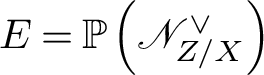 $E = \mathbb {P}\left (\mathscr {N}_{Z/X}^\vee \right )$
is a projective bundle over Z. We have a Cartesian diagram
$E = \mathbb {P}\left (\mathscr {N}_{Z/X}^\vee \right )$
is a projective bundle over Z. We have a Cartesian diagram

The excess bundle
 $\mathscr {V}$
for the diagram is defined by the short exact sequence
$\mathscr {V}$
for the diagram is defined by the short exact sequence
 $$ \begin{align*} 0 \to \mathscr{N}_{E/\widetilde{X}} \to p^*\mathscr{N}_{Z/X} \to \mathscr{V} \to 0. \end{align*} $$
From the excess bundle formula [Reference Fulton18, Theorem 6.3], one obtains the key formula for blowup:
 $$ \begin{align} \pi^* i_* (\underline{\hphantom{A}}) = j_* (c_{r-1}(\mathscr{V}) \cap p^*(\underline{\hphantom{A}})) \colon \operatorname{CH}_{k}(Z) \to \operatorname{CH}_k\left(\widetilde{X}\right). \end{align} $$
The following is summarized from [Reference Fulton18, Proposition 6.7]:
Theorem 2.8 blowups
-
(1) The following hold:
$$ \begin{align*} \pi_* \pi^* = \operatorname{Id}_{\operatorname{CH}(X)}, \qquad p_*(c_{r-1}(\mathscr{V}) \cap p^*(\underline{\hphantom{A}})) = \operatorname{Id}_{\operatorname{CH}(Z)}. \end{align*} $$
-
(2) For any
$k \ge 0$
, there exists a split short exact sequence where a left inverse of the first map is given by
$$ \begin{align*} 0 \to \operatorname{CH}_{k}(Z) \xrightarrow{\left(c_{r-1}(\mathscr{V}) \cap p^*(\underline{\hphantom{A}}), -i_*\right)} \operatorname{CH}_{k}(E) \oplus \operatorname{CH}_{k}(X) \xrightarrow{\left(\varepsilon, \alpha\right) \mapsto j_*\varepsilon + \pi^* \alpha} \operatorname{CH}_k\left(\widetilde{X}\right) \to 0, \end{align*} $$
$(\varepsilon , \alpha ) \mapsto p_* \varepsilon $
.
-
(3) This exact sequence induces an isomorphism of Chow groups
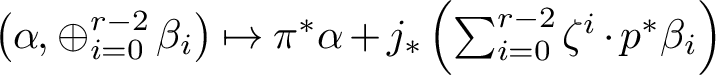
given by
$$ \begin{align*} \operatorname{CH}_{k}(X) \oplus \bigoplus_{i=0}^{r-2} \operatorname{CH}_{k-(r-1)+i}(Z) \xrightarrow{\sim} \operatorname{CH}_{k}\left(\widetilde{X}\right), \end{align*} $$
$\left (\alpha , \oplus _{i=0}^{r-2} \beta _i\right ) \mapsto \pi ^* \alpha + j_*\left (\sum _{i=0}^{r-2} \zeta ^i \cdot p^*\beta _i\right )$
, where
$\zeta = c_1\left (\mathscr {O}_{\mathbb {P}\left (\mathscr {N}_{Z/X}^\vee \right )}(1)\right )$
.


Note that the well-known formula of part (3) follows from part (2) by the identification
 $$ \begin{align*} \operatorname{CH}_{k}\left(\widetilde{X}\right) & = \pi^* \operatorname{CH}_{k}(X) \oplus j_* \left(\operatorname{CH}_k(E)_{p_*=0}\right) \\ &= \pi^* \operatorname{CH}_{k}(X) \oplus \bigoplus_{i=0}^{r-2} j_* \left(\zeta^ i \cdot p^*\operatorname{CH}_{k-(r-1)+i}(Z)\right), \end{align*} $$
where
 $\operatorname {CH}_k(E)_{p_*=0}$
denotes the subgroup
$\operatorname {CH}_k(E)_{p_*=0}$
denotes the subgroup
 $\{\gamma \in \operatorname {CH}_k(E) \mid p_* \gamma = 0\}$
of
$\{\gamma \in \operatorname {CH}_k(E) \mid p_* \gamma = 0\}$
of
 $\operatorname {CH}_k(E)$
. A similar and more detailed argument is given later in the case of standard flips (see Theorem 3.6). There are similar results on Chow motives by Manin [Reference Manin39] (see also our Corollary 3.10).
$\operatorname {CH}_k(E)$
. A similar and more detailed argument is given later in the case of standard flips (see Theorem 3.6). There are similar results on Chow motives by Manin [Reference Manin39] (see also our Corollary 3.10).
3 The Cayley trick and standard flips
The projectivization can be viewed as a combination of the situation of the Cayley trick and flips. In this section we study the Chow theory of the latter two cases.
3.1 The Cayley trick and Chow groups
The Cayley trick is a method to relate the geometry of the zero scheme of a regular section of a vector bundle to the geometry of a hypersurface (see the discussions of [Reference Jiang, Leung and Xie25, §2.3]). The relationships for their derived categories were established by Orlov [Reference Orlov46, Proposition 2.10]; we now focus on their Chow groups.
Let
 $\mathscr {E}$
be a locally free sheaf of rank
$\mathscr {E}$
be a locally free sheaf of rank
 $r \ge 2$
on a scheme X and
$r \ge 2$
on a scheme X and
 $s \in H^0(X,\mathscr {E})$
be a regular section, and denote
$s \in H^0(X,\mathscr {E})$
be a regular section, and denote
 $Z:=Z(s)$
the zero locus of the section s. Denote the projectivization by
$Z:=Z(s)$
the zero locus of the section s. Denote the projectivization by
 $q\colon \mathbb {P}(\mathscr {E}) = \operatorname {Proj} \operatorname {Sym}^\bullet \mathscr {E} \to X$
. Then under the canonical identification
$q\colon \mathbb {P}(\mathscr {E}) = \operatorname {Proj} \operatorname {Sym}^\bullet \mathscr {E} \to X$
. Then under the canonical identification
 $$ \begin{align*} H^0(X,\mathscr{E}) = H^0\left(\mathbb{P}(\mathscr{E}), \mathscr{O}_{\mathbb{P}(\mathscr{E})}(1)\right), \end{align*} $$
the section s corresponds canonically to a section
 $f_s$
of
$f_s$
of
 $\mathscr {O}_{\mathbb {P}(\mathscr {E})}(1)$
on
$\mathscr {O}_{\mathbb {P}(\mathscr {E})}(1)$
on
 $\mathbb {P}(\mathscr {E})$
. Denote the divisor defined by
$\mathbb {P}(\mathscr {E})$
. Denote the divisor defined by
 $f_s$
by
$f_s$
by
 $$ \begin{align*} \mathcal{H}_s : = Z(f_s) \subset \mathbb{P}(\mathscr{E}). \end{align*} $$
Then
 $\mathcal {H}_s = \mathbb {P}(\mathscr {G}) = \operatorname {Proj} \operatorname {Sym}^\bullet \mathscr {G}$
, where
$\mathcal {H}_s = \mathbb {P}(\mathscr {G}) = \operatorname {Proj} \operatorname {Sym}^\bullet \mathscr {G}$
, where
 $\mathscr {G} = \operatorname {Coker}\left (\mathscr {O}_X \xrightarrow {~s~} \mathscr {E}\right )$
. Thus
$\mathscr {G} = \operatorname {Coker}\left (\mathscr {O}_X \xrightarrow {~s~} \mathscr {E}\right )$
. Thus
 $\mathcal {H}_s$
is a
$\mathcal {H}_s$
is a
 $\mathbb {P}^{r-2}$
-bundle over
$\mathbb {P}^{r-2}$
-bundle over
 $X \backslash Z$
, and a
$X \backslash Z$
, and a
 $\mathbb {P}^{r-1}$
-bundle over Z. It follows that
$\mathbb {P}^{r-1}$
-bundle over Z. It follows that
 $\mathcal {H}_s\rvert _{Z}$
coincides with
$\mathcal {H}_s\rvert _{Z}$
coincides with
 $\mathbb {P}_Z(\mathscr {N}_i)$
, the projectivization of the normal bundle of inclusion
$\mathbb {P}_Z(\mathscr {N}_i)$
, the projectivization of the normal bundle of inclusion
 $i \colon Z \hookrightarrow X$
. The situation is illustrated in the following commutative diagram, with maps as labeled:
$i \colon Z \hookrightarrow X$
. The situation is illustrated in the following commutative diagram, with maps as labeled:

Since
 $\mathscr {N}_i = \mathscr {E}\rvert _{Z}$
and
$\mathscr {N}_i = \mathscr {E}\rvert _{Z}$
and
 $\mathscr {O}_{\mathbb {P}(\mathscr {E})}(1)\rvert _{\mathbb {P}(\mathscr {N}_i)} = \mathscr {O}_{\mathbb {P}\left (\mathscr {N}_i\right )}(1)$
, by abuse of notation we use
$\mathscr {O}_{\mathbb {P}(\mathscr {E})}(1)\rvert _{\mathbb {P}(\mathscr {N}_i)} = \mathscr {O}_{\mathbb {P}\left (\mathscr {N}_i\right )}(1)$
, by abuse of notation we use
 $\zeta \cdot (\underline {\hphantom {A}})$
to denote both
$\zeta \cdot (\underline {\hphantom {A}})$
to denote both
 $c_1\left (\mathscr {O}_{\mathbb {P}(\mathscr {E})}(1)\right )\cap (\underline {\hphantom {A}})$
and
$c_1\left (\mathscr {O}_{\mathbb {P}(\mathscr {E})}(1)\right )\cap (\underline {\hphantom {A}})$
and
 $c_1\left (\mathscr {O}_{\mathbb {P}\left (\mathscr {N}_i\right )}(1)\right )\cap (\underline {\hphantom {A}})$
. The main result of this section is the following:
$c_1\left (\mathscr {O}_{\mathbb {P}\left (\mathscr {N}_i\right )}(1)\right )\cap (\underline {\hphantom {A}})$
. The main result of this section is the following:
Theorem 3.1 the Cayley trick for Chow groups
There exists a split short exact sequence
 $$ \begin{align} 0 \to \bigoplus_{i=0}^{r-2} \operatorname{CH}_{k-(r-2)+i}(Z) \xrightarrow{f} \bigoplus_{i=0}^{r-2} \operatorname{CH}_{k-(r-2)+i}(X) \oplus \operatorname{CH}_{k}(\mathbb{P}(\mathscr{N}_i)) \xrightarrow{g} \operatorname{CH}_k(\mathcal{H}_s) \to 0, \end{align} $$
where the maps f and g are given by
 $$ \begin{align*} f & \colon \oplus_{i=0}^{r-2} \gamma_i \mapsto \left(- \oplus_{i=0}^{r-2} i_* \gamma_i , \sum_{i=0}^{r-2} \zeta^{i+1} \cdot p^* \gamma_i\right), \\ g & \colon \left(\oplus_{i=0}^{r-2} \alpha_i, \varepsilon\right) \mapsto \sum_{i=0}^{r-2} \zeta^i \cdot \pi^*\alpha_i + j_* \varepsilon, \end{align*} $$
where
 $p_{i*}$
is defined similarly to equation (2.1). A left inverse of f is given by
$p_{i*}$
is defined similarly to equation (2.1). A left inverse of f is given by
 $\left (\oplus _{i=0}^{r-2} \alpha _i, \varepsilon \right ) \mapsto \oplus _{i=0}^{r-2} p_{i+1*} \varepsilon $
. Furthermore, the sequence induces an isomorphism
$\left (\oplus _{i=0}^{r-2} \alpha _i, \varepsilon \right ) \mapsto \oplus _{i=0}^{r-2} p_{i+1*} \varepsilon $
. Furthermore, the sequence induces an isomorphism
 $$ \begin{align} \bigoplus_{i=0}^{r-2} \operatorname{CH}_{k-(r-2)+i}(X) \oplus \operatorname{CH}_{k-(r-1)}(Z) \xrightarrow{\sim} \operatorname{CH}_{k}(\mathcal{H}_s), \end{align} $$
given by
 $\left (\oplus _{i=0}^{r-2} \alpha _i, \gamma \right ) \mapsto \sum _{i=0}^{r-2} \zeta ^i \cdot \pi ^*\alpha _i + j_* p^* \gamma $
, and in this decomposition the projection map to the first
$\left (\oplus _{i=0}^{r-2} \alpha _i, \gamma \right ) \mapsto \sum _{i=0}^{r-2} \zeta ^i \cdot \pi ^*\alpha _i + j_* p^* \gamma $
, and in this decomposition the projection map to the first
 $(r-1)$
-summands
$(r-1)$
-summands
 $\operatorname {CH}_{k}(\mathcal {H}_s) \to \operatorname {CH}_{k-(r-2)+i}(X)$
,
$\operatorname {CH}_{k}(\mathcal {H}_s) \to \operatorname {CH}_{k-(r-2)+i}(X)$
,
 $i=0,1,\dotsc , r-2$
, is given by
$i=0,1,\dotsc , r-2$
, is given by
 $\beta \mapsto \pi _{i*} \beta $
, where
$\beta \mapsto \pi _{i*} \beta $
, where
 $\pi _{i*}$
is defined by equation (3.4) and the projection to the last summand
$\pi _{i*}$
is defined by equation (3.4) and the projection to the last summand
 $\operatorname {CH}_{k}(\mathcal {H}_s) \to \operatorname {CH}_{k-(r-1)}(Z)$
is given by
$\operatorname {CH}_{k}(\mathcal {H}_s) \to \operatorname {CH}_{k-(r-1)}(Z)$
is given by
 $\beta \mapsto (-1)^{r-1} p_* j^*\beta $
.
$\beta \mapsto (-1)^{r-1} p_* j^*\beta $
.
For simplicity, we introduce the following notation. For the projective bundles
 $q: \mathbb {P}(\mathscr {E}) \to X$
and
$q: \mathbb {P}(\mathscr {E}) \to X$
and
 $p: \mathbb {P}(\mathscr {N}_i) \to Z$
, similar to equation (2.1), we denote the projections to the ith factors by
$p: \mathbb {P}(\mathscr {N}_i) \to Z$
, similar to equation (2.1), we denote the projections to the ith factors by
 $$ \begin{align*} q_{i*} \colon \operatorname{CH}_k(\mathbb{P}(\mathscr{E})) \to \operatorname{CH}_{k-(r-1)+i}(X), \qquad p_{i*} \colon \operatorname{CH}_k(\mathbb{P}(\mathscr{N}_i)) \to \operatorname{CH}_{k-(r-1)+i}(Z), \end{align*} $$
which are explicitly given as follows: for any
 $i=0,1,\dotsc , r-1$
,
$i=0,1,\dotsc , r-1$
,
 $$ \begin{align*} q_{i*} (\underline{\hphantom{A}})& = \sum_{j=0}^{r-1-i} (-1)^jc_{j}(\mathscr{E}) \cap q_* \left(\zeta^{r-1-i-j} \cdot (\underline{\hphantom{A}}) \right), \\ p_{i*} (\underline{\hphantom{A}})& = \sum_{j=0}^{r-1-i} (-1)^jc_{j}(\mathscr{N}_i) \cap p_* \left(\zeta^{r-1-i-j} \cdot (\underline{\hphantom{A}})\right). \end{align*} $$
Furthermore, for any
 $i \in [0,r-1]$
,
$i \in [0,r-1]$
,
 $\alpha \in \operatorname {CH}(X)$
, and
$\alpha \in \operatorname {CH}(X)$
, and
 $\gamma \in \operatorname {CH}(Z)$
, we denote
$\gamma \in \operatorname {CH}(Z)$
, we denote
 $$ \begin{align*} q_i^* \alpha: = \zeta^i \cdot q^*\alpha, \qquad p_i^* \gamma := \zeta^i \cdot p^* \gamma. \end{align*} $$
Then the projective bundle formula (Theorem 2.4) states the following:
-
(1) For all
$i,j \in [0,r-1]$
,
$$ \begin{align*} q_{i *} q_j^* = \delta_{i,j} \operatorname{Id}_{\operatorname{CH}(X)}, \qquad p_{i *} p_j^* = \delta_{i,j} \operatorname{Id}_{\operatorname{CH}(Z)}. \end{align*} $$
-
(2) For all
$\beta \in \operatorname {CH}(\mathbb {P}(\mathscr {E}))$
and
$\varepsilon \in \operatorname {CH}(\mathbb {P}(\mathscr {N}_i))$
, the following relations hold:
$$ \begin{align*} \beta = \sum_{i=0}^{r-1} q_i^* q_{i*} \beta \qquad \varepsilon = \sum_{i=0}^{r-1} p^*_i p_{i*} \varepsilon. \end{align*} $$


Now for all
 $\alpha \in \operatorname {CH}_{\ell }(X)$
and
$\alpha \in \operatorname {CH}_{\ell }(X)$
and
 $\beta \in \operatorname {CH}_k(\mathcal {H}_s)$
, and all
$\beta \in \operatorname {CH}_k(\mathcal {H}_s)$
, and all
 $i \in [0,r-2]$
, we define
$i \in [0,r-2]$
, we define
 $$ \begin{align*} \pi_i^*\alpha : = \iota^* q_i^* \alpha \in \operatorname{CH}_{\ell+(r-2)-i}(\mathcal{H}_s), \qquad \pi_{i*} \beta : = q_{i+1*} \iota_* \beta \in \operatorname{CH}_{k-(r-2)+i}(X). \end{align*} $$
Then it follows from the projection formula that
 $\pi _i^* \alpha = \zeta ^i \cdot \pi ^* \alpha $
, and
$\pi _i^* \alpha = \zeta ^i \cdot \pi ^* \alpha $
, and
 $\pi _{r-2*} = \pi _*$
and
$\pi _{r-2*} = \pi _*$
and
 $$ \begin{align} \pi_{i*} (\underline{\hphantom{A}})= \sum_{j=0}^{r-2-i} (-1)^jc_{j}(\mathscr{E}) \cap \pi_* \left(\zeta^{r-2-i-j} \cdot (\underline{\hphantom{A}}) \right), \qquad i=0,\dotsc, r-2. \end{align} $$
Notice that
 $c_{i}(\mathscr {E}) =c_{i}(\mathscr {G})$
for
$c_{i}(\mathscr {E}) =c_{i}(\mathscr {G})$
for
 $i \in [0,r-2]$
, where
$i \in [0,r-2]$
, where
 $\mathscr {G} = \operatorname {Coker}\left (\mathscr {O}_X \xrightarrow {~s~} \mathscr {E}\right )$
; the relationships between
$\mathscr {G} = \operatorname {Coker}\left (\mathscr {O}_X \xrightarrow {~s~} \mathscr {E}\right )$
; the relationships between
 $\pi _{i*}$
s and
$\pi _{i*}$
s and
 $\pi _i^*$
s are similar to the case of a
$\pi _i^*$
s are similar to the case of a
 $\mathbb {P}^{r-2}$
-bundle.
$\mathbb {P}^{r-2}$
-bundle.
We prove the theorem by the same steps as the blowup case in [Reference Fulton18, §6.7]:
Proposition 3.2 compare [Reference Fulton18, Proposition 6.7]
-
(a) (Key formula). For all
$\alpha \in \operatorname {CH}_k(Z)$
, Then by the projection formula,
$$ \begin{align*} \pi^* i_* \alpha = j_* (\zeta \cdot p^* \alpha) \in \operatorname{CH}_{k+r-2}(\mathcal{H}_s). \end{align*} $$
$\pi _i^* i_* \alpha = j_* \left (\zeta \cdot p_i^* \alpha \right )$
for all
$i\in [0,r-2]$
.
-
(b) For any
$\alpha \in \operatorname {CH}_k(X)$
,
$i,j \in [0,r-2]$
, we have
$\pi _{i*} \pi _i^* \alpha = \alpha $
,
$\pi _{i*} \pi _j^* \alpha =0$
if
$i \ne j$
. -
(c) For
$\varepsilon \in \operatorname {CH}(\mathbb {P}(\mathscr {N}_i))$
, if
$j^*j_*\varepsilon = 0$
and
$p_{1*} \varepsilon = \dotsb = p_{r-1*} \varepsilon =0$
, then
$\varepsilon = 0$
. -
(d)
-
(i) For any
$\beta \in \operatorname {CH}_k(\mathcal {H}_s)$
, there is an
$\varepsilon \in \operatorname {CH}_k(\mathbb {P}(\mathscr {N}_i))$
such that
$$ \begin{align*} \beta = \sum_{i=0}^{r-2} \pi_i^* \pi_{i*} \beta + j_* \varepsilon. \end{align*} $$
-
(ii) For any
$\beta \in \operatorname {CH}_k(\mathcal {H}_s)$
, if
$\pi _{i *} \beta = 0$
,
$i \in [0,r-2]$
, and
$j^* \beta = 0$
, then
$\beta =0$
.
-


Proof. (a) In fact, from [Reference Jiang, Leung and Xie25, Remark. 2.5], the Euler sequence for
 $\mathbb {P}(\mathscr {N}_i)$
is equivalent to
$\mathbb {P}(\mathscr {N}_i)$
is equivalent to
 $$ \begin{align} 0 \to \mathscr{N}_j \to p^* \mathscr{N}_i \to \mathscr{O}_{\mathbb{P}\left(\mathscr{N}_i\right)}(1) \to 0, \end{align} $$
where
 $\mathscr {N}_i = \mathscr {E}\rvert _Z$
and
$\mathscr {N}_i = \mathscr {E}\rvert _Z$
and
 $\mathscr {N}_j \simeq \Omega _{\mathbb {P}(\mathscr {E})/X}(1)\rvert _{\mathbb {P}\left (\mathscr {N}_i\right )}$
. Therefore the excess bundle for diagram 3.1 is given by
$\mathscr {N}_j \simeq \Omega _{\mathbb {P}(\mathscr {E})/X}(1)\rvert _{\mathbb {P}\left (\mathscr {N}_i\right )}$
. Therefore the excess bundle for diagram 3.1 is given by
 $ \mathscr {O}_{\mathbb {P}\left (\mathscr {N}_i\right )}(1)$
. Now from [Reference Fulton18, Theorem 6.3, Propositions 6.2(1) and 6.6], one has:
$ \mathscr {O}_{\mathbb {P}\left (\mathscr {N}_i\right )}(1)$
. Now from [Reference Fulton18, Theorem 6.3, Propositions 6.2(1) and 6.6], one has:
 $$ \begin{align*} \pi^* i_* (\underline{\hphantom{A}}) = j_* \pi^!_{\mathbb{P}\left(\mathscr{N}_i\right)} (\underline{\hphantom{A}}) = j_* \left(c_1\left(\mathscr{O}_{\mathbb{P}\left(\mathscr{N}_i\right)}(1)\right) \cap p^*(\underline{\hphantom{A}})\right). \end{align*} $$
(b) Since
 $\iota \colon \mathcal {H}_s \hookrightarrow \mathbb {P}(\mathscr {E})$
is a divisor of
$\iota \colon \mathcal {H}_s \hookrightarrow \mathbb {P}(\mathscr {E})$
is a divisor of
 $\mathscr {O}_{\mathbb {P}(\mathscr {E})}(1)$
, we have
$\mathscr {O}_{\mathbb {P}(\mathscr {E})}(1)$
, we have
 $\iota ^* \iota _* (\underline {\hphantom {A}}) = \zeta \cdot (\underline {\hphantom {A}})$
, and
$\iota ^* \iota _* (\underline {\hphantom {A}}) = \zeta \cdot (\underline {\hphantom {A}})$
, and
 $$ \begin{align*} \pi_{i*} \pi_j^* \alpha = q_{i+1*} \iota_* \left( \iota^* \left(q_j^* \alpha\right) \right) = q_{i+1*} \left(\zeta \cdot \zeta^j \cdot q^* \alpha\right) = q_{i+1*} q_{j+1}^* \alpha =\delta_{i,j} \alpha. \end{align*} $$
(c) Since
 $j^*j_*\varepsilon = c_{r-1}\left (\mathscr {N}_j\right ) \cap \varepsilon $
, from the Euler sequence (3.5) and
$j^*j_*\varepsilon = c_{r-1}\left (\mathscr {N}_j\right ) \cap \varepsilon $
, from the Euler sequence (3.5) and
 $\mathscr {N}_i = \mathscr {E}\rvert _Z$
,
$\mathscr {N}_i = \mathscr {E}\rvert _Z$
,
 $$ \begin{align*} c_{r-1}(\mathscr{N}_j) = \sum_{i=0}^{r-1} (-1)^i \zeta^i p^* c_{r-1-i}(\mathscr{E}) = (-1)^{r-1} \zeta^{r-1} + \text{(lower order terms of}\ \zeta^{i}). \end{align*} $$
Therefore
 $j^*j_*\varepsilon = c_{r-1}\left (\mathscr {N}_j\right ) \cap \varepsilon = 0$
and
$j^*j_*\varepsilon = c_{r-1}\left (\mathscr {N}_j\right ) \cap \varepsilon = 0$
and
 $p_{1*} \varepsilon = \dotsb = p_{r-1*} \varepsilon =0$
imply
$p_{1*} \varepsilon = \dotsb = p_{r-1*} \varepsilon =0$
imply
 $p_{0 *} \varepsilon = p_*\left (\zeta ^{r-1} \cdot \varepsilon \right ) + p_* \left (\left (\text {lower-order terms of }\zeta ^{i}\right ) \cap \varepsilon \right ) = \pm p_*\left ( c_{r-1}\left (\mathscr {N}_j\right ) \cap \varepsilon \right ) + p_* \left (\left (\text {lower-order terms of }\zeta ^{i}\right )\right. \left.\cap \varepsilon \right ) = 0$
. Hence
$p_{0 *} \varepsilon = p_*\left (\zeta ^{r-1} \cdot \varepsilon \right ) + p_* \left (\left (\text {lower-order terms of }\zeta ^{i}\right ) \cap \varepsilon \right ) = \pm p_*\left ( c_{r-1}\left (\mathscr {N}_j\right ) \cap \varepsilon \right ) + p_* \left (\left (\text {lower-order terms of }\zeta ^{i}\right )\right. \left.\cap \varepsilon \right ) = 0$
. Hence
 $\varepsilon = \sum _{i=0}^{r-1} p_i^* p_{i*} \varepsilon = 0$
.
$\varepsilon = \sum _{i=0}^{r-1} p_i^* p_{i*} \varepsilon = 0$
.
(d)(i) Over the open subscheme
 $U = X \backslash Z$
,
$U = X \backslash Z$
,
 $\mathcal {H}_s\rvert _{\pi ^{-1}(U)} = \mathbb {P}(\mathscr {G}\rvert _U)$
is a projective bundle with fiber
$\mathcal {H}_s\rvert _{\pi ^{-1}(U)} = \mathbb {P}(\mathscr {G}\rvert _U)$
is a projective bundle with fiber
 $\mathbb {P}^{r-2}$
. In fact, over U there is an exact sequence of vector bundles
$\mathbb {P}^{r-2}$
. In fact, over U there is an exact sequence of vector bundles
 $0 \to \mathscr {O}_U \to \mathscr {E}\rvert _U \to \mathscr {G}\rvert _U \to 0$
. Then the linear subbundle
$0 \to \mathscr {O}_U \to \mathscr {E}\rvert _U \to \mathscr {G}\rvert _U \to 0$
. Then the linear subbundle
 $\mathbb {P}( \mathscr {G}\rvert _U) \subset \mathbb {P}(\mathscr {E}\rvert _U)$
is a divisor representing the class
$\mathbb {P}( \mathscr {G}\rvert _U) \subset \mathbb {P}(\mathscr {E}\rvert _U)$
is a divisor representing the class
 $\zeta = c_1 (\mathscr {O}(1))$
. For any
$\zeta = c_1 (\mathscr {O}(1))$
. For any
 $\beta \in \operatorname {CH}(\mathbb {P}( \mathscr {G}\rvert _U))$
, by Theorem 2.4 applied to
$\beta \in \operatorname {CH}(\mathbb {P}( \mathscr {G}\rvert _U))$
, by Theorem 2.4 applied to
 $\mathbb {P}(\mathscr {G}_U)$
there exists a unique
$\mathbb {P}(\mathscr {G}_U)$
there exists a unique
 $\alpha _i \in \operatorname {CH}(U)$
such that
$\alpha _i \in \operatorname {CH}(U)$
such that
 $\beta = \sum _{i=0}^{r-2} (\iota ^*\zeta )^i \cdot \pi ^* \alpha _i$
. Therefore the following holds:
$\beta = \sum _{i=0}^{r-2} (\iota ^*\zeta )^i \cdot \pi ^* \alpha _i$
. Therefore the following holds:
 $$ \begin{align*} \iota_* \beta = \sum_{i=0}^{r-2} \iota_* \left(\left(\iota^*(\zeta)^i \cdot \iota^*(q^* \alpha)\right)\right. = \sum_{i=0}^{r-2} \zeta^{i+1} \cdot q^* \alpha_i, \end{align*} $$
where the last equality follows from the projection formula and
 $\iota _* \iota ^* (\underline {\hphantom {A}}) = \zeta \cdot (\underline {\hphantom {A}})$
. From the uniqueness statement of Theorem 2.4 applied to
$\iota _* \iota ^* (\underline {\hphantom {A}}) = \zeta \cdot (\underline {\hphantom {A}})$
. From the uniqueness statement of Theorem 2.4 applied to
 $\mathbb {P}(\mathscr {E})$
, we know that
$\mathbb {P}(\mathscr {E})$
, we know that
 $$ \begin{align*} \alpha_i = q_{i+1*} \iota_* \beta = \pi_{i *} \beta. \end{align*} $$
Therefore, over U, we have
 $\beta = \sum _{i=0}^{r-2} \pi _i^* \pi _{i*} \beta .$
Now for any
$\beta = \sum _{i=0}^{r-2} \pi _i^* \pi _{i*} \beta .$
Now for any
 $\beta \in \operatorname {CH}_k(\mathcal {H}_s)$
,
$\beta \in \operatorname {CH}_k(\mathcal {H}_s)$
,
 $\left (\beta - \sum _{i=0}^{r-2} \pi _i^* \pi _{i*} \beta \right )\big \rvert _U = 0$
. From the exact sequence
$\left (\beta - \sum _{i=0}^{r-2} \pi _i^* \pi _{i*} \beta \right )\big \rvert _U = 0$
. From the exact sequence
 $\operatorname {CH}(\mathbb {P}(\mathscr {N}_i)) \to \operatorname {CH}(\mathcal {H}_s) \to \operatorname {CH}(\mathcal {H}_{s}\rvert _U) \to 0$
, there exists an
$\operatorname {CH}(\mathbb {P}(\mathscr {N}_i)) \to \operatorname {CH}(\mathcal {H}_s) \to \operatorname {CH}(\mathcal {H}_{s}\rvert _U) \to 0$
, there exists an
 $\varepsilon \in \operatorname {CH}(\mathbb {P}(\mathscr {N}_i))$
such that
$\varepsilon \in \operatorname {CH}(\mathbb {P}(\mathscr {N}_i))$
such that
 $\beta - \sum _{i=0}^{r-2} \pi _i^* \pi _{i*} \beta = j_* \varepsilon $
.
$\beta - \sum _{i=0}^{r-2} \pi _i^* \pi _{i*} \beta = j_* \varepsilon $
.
(d)(ii) From part (d)(i) we know that
 $\beta = j_* \varepsilon $
, for
$\beta = j_* \varepsilon $
, for
 $\varepsilon \in \operatorname {CH}_k(\mathbb {P}(\mathscr {N}_i))$
. Since the ambient square of diagram (3.1) is flat, by the flat base-change formula we have
$\varepsilon \in \operatorname {CH}_k(\mathbb {P}(\mathscr {N}_i))$
. Since the ambient square of diagram (3.1) is flat, by the flat base-change formula we have
 $$ \begin{align*} i_* p_{i+1 *} = q_{i+1 *} (\iota \circ j)_* = \pi_{i *} j_*, \qquad \text{for } i = 0,1,\dotsc, r-2. \end{align*} $$
Therefore
 $i_* (p_{i+1 *} \varepsilon ) = \pi _{i } * \beta = 0$
for
$i_* (p_{i+1 *} \varepsilon ) = \pi _{i } * \beta = 0$
for
 $i \in [0,r-2]$
. Notice that since
$i \in [0,r-2]$
. Notice that since
 $\varepsilon = \sum _{i=0}^{r-1} p_i^* p_{i *} \varepsilon $
, one has
$\varepsilon = \sum _{i=0}^{r-1} p_i^* p_{i *} \varepsilon $
, one has
 $$ \begin{align*} j_* \left(p_0^* p_{0*} \varepsilon\right) = j_*( \varepsilon) - j_* \left(\zeta \cdot \sum_{i=0}^{r-2} p_{i}^* p_{i+1 *} \varepsilon \right) = j_*( \varepsilon) - \sum_{i=0}^{r-2} \pi_{i}^* i_* (p_{i+1 *} \varepsilon) = j_*( \varepsilon). \end{align*} $$
Here the second equality follows from the key formula of part (a). Now
 $j^* j_* \left (p_0^* p_{0*} \varepsilon \right ) = j^* j_* \varepsilon =0$
. By part (c),
$j^* j_* \left (p_0^* p_{0*} \varepsilon \right ) = j^* j_* \varepsilon =0$
. By part (c),
 $p_0^* p_{0*} \varepsilon =0$
, hence
$p_0^* p_{0*} \varepsilon =0$
, hence
 $\beta = j_* \varepsilon =0$
.
$\beta = j_* \varepsilon =0$
.
Theorem 3.1 follows from Proposition 3.2 as follows:
Proof of Theorem 3.1. The fact
 $gf =0$
follows from part (a). The surjectivity of g is part (d)(i). By part (b), a left inverse of f is given by
$gf =0$
follows from part (a). The surjectivity of g is part (d)(i). By part (b), a left inverse of f is given by
 $h \colon \left (\oplus _{i=0}^{r-2} \alpha _i, \varepsilon \right ) \mapsto \oplus _{i=0}^{r-2} p_{i+1*} \varepsilon .$
In fact,
$h \colon \left (\oplus _{i=0}^{r-2} \alpha _i, \varepsilon \right ) \mapsto \oplus _{i=0}^{r-2} p_{i+1*} \varepsilon .$
In fact,
 $hf$
is
$hf$
is
 $$ \begin{align*} \oplus_{i=0}^{r-2} \gamma_i \mapsto \oplus_{i=0}^{r-2} p_{i+1*} \left(\sum_{j=0}^{r-2} \zeta^{j+1} \cdot p^* \gamma_j\right) = \oplus_{i=0}^{r-2} \left(p_{i+1*} \sum_{j=0}^{r-2} p_{j+1}^* \gamma_i\right) = \oplus_{i=0}^{r-2} \gamma_i. \end{align*} $$
To show the exactness of formula (3.2), suppose that for
 $\alpha _i \in \operatorname {CH}(X)$
and
$\alpha _i \in \operatorname {CH}(X)$
and
 $\varepsilon \in \operatorname {CH}(\mathbb {P}(\mathscr {N}_i))$
, we have
$\varepsilon \in \operatorname {CH}(\mathbb {P}(\mathscr {N}_i))$
, we have
 $\sum _{i=0}^{r-2} \pi _i^* \alpha _i + j_* \varepsilon = 0.$
Then similar to part (d)(ii), from part (b), for all
$\sum _{i=0}^{r-2} \pi _i^* \alpha _i + j_* \varepsilon = 0.$
Then similar to part (d)(ii), from part (b), for all
 $i \in [0,r-2]$
,
$i \in [0,r-2]$
,
 $$ \begin{align*} \alpha_i = - \pi_{i*} ( j_* \varepsilon) = - i_{*} p_{i+1*} \varepsilon \in \operatorname{CH}(X). \end{align*} $$
Now consider
 $ \varepsilon ^{\prime } = \varepsilon - \sum _{i=0}^{r-2} p_{i+1}^* p_{i+1*} \varepsilon. $
Then similar to the proof of part (d)(ii), we have
$ \varepsilon ^{\prime } = \varepsilon - \sum _{i=0}^{r-2} p_{i+1}^* p_{i+1*} \varepsilon. $
Then similar to the proof of part (d)(ii), we have
 $$ \begin{align*} j_* \varepsilon^{\prime} = j_*( \varepsilon) - j_* \left(\zeta \cdot \sum_{i=0}^{r-2} p_{i}^* p_{i+1 *} \varepsilon \right) = j_*( \varepsilon) - \sum_{i=0}^{r-2} \pi_{i}^* i_* (p_{i+1 *} \varepsilon) = j_*( \varepsilon) + \sum_{i=0}^{r-2} \pi_{i}^* \alpha_i =0, \end{align*} $$
and
 $p_{1*} \varepsilon ^{\prime } = \dotsb = p_{r-1*} \varepsilon ^{\prime } =0$
(since
$p_{1*} \varepsilon ^{\prime } = \dotsb = p_{r-1*} \varepsilon ^{\prime } =0$
(since
 $\varepsilon ^{\prime } =p_0^* p_{0*} \varepsilon $
). Therefore by part (c),
$\varepsilon ^{\prime } =p_0^* p_{0*} \varepsilon $
). Therefore by part (c),
 $ \varepsilon ^{\prime } =0$
. Hence
$ \varepsilon ^{\prime } =0$
. Hence
 $(\oplus _i \alpha _i, \varepsilon ) = \left ( -\oplus _i i_{*} \gamma _i, \sum _{i=0}^{r-2} p_{i+1}^*\gamma _i\right )$
for
$(\oplus _i \alpha _i, \varepsilon ) = \left ( -\oplus _i i_{*} \gamma _i, \sum _{i=0}^{r-2} p_{i+1}^*\gamma _i\right )$
for
 $\gamma _i= p_{i+1*} \varepsilon $
. Hence the sequence (3.2) is exact.
$\gamma _i= p_{i+1*} \varepsilon $
. Hence the sequence (3.2) is exact.
To prove the last statement, we show that for any
 $\beta \in \operatorname {CH}(\mathcal {H}_s)$
, there exists a unique
$\beta \in \operatorname {CH}(\mathcal {H}_s)$
, there exists a unique
 $\varepsilon \in \operatorname {CH}(\mathbb {P}(\mathscr {N}_i))$
such that
$\varepsilon \in \operatorname {CH}(\mathbb {P}(\mathscr {N}_i))$
such that
 $p_{1*} \varepsilon = \dotsb = p_{r-1*} \varepsilon =0$
, and
$p_{1*} \varepsilon = \dotsb = p_{r-1*} \varepsilon =0$
, and
 $$ \begin{align*} \beta = \sum_{i=0}^{r-2} \pi_i^* \pi_{i*} \beta + j_* \varepsilon. \end{align*} $$
In fact, for any expression
 $\beta = \sum _{i=0}^{r-2} \pi _i^* \alpha _i + j_* \varepsilon ,$
by replacing
$\beta = \sum _{i=0}^{r-2} \pi _i^* \alpha _i + j_* \varepsilon ,$
by replacing
 $\varepsilon $
with
$\varepsilon $
with
 $\varepsilon - \sum _{i=0}^{r-2} p_{i+1}^* p_{i+1*} \varepsilon $
and
$\varepsilon - \sum _{i=0}^{r-2} p_{i+1}^* p_{i+1*} \varepsilon $
and
 $\alpha _i$
with
$\alpha _i$
with
 $\alpha _i+ i_* (p_{i+1 *} \varepsilon )$
, we may assume
$\alpha _i+ i_* (p_{i+1 *} \varepsilon )$
, we may assume
 $p_{1*} \varepsilon = \dotsb = p_{r-1*} \varepsilon =0$
. Hence by the projective bundle formula,
$p_{1*} \varepsilon = \dotsb = p_{r-1*} \varepsilon =0$
. Hence by the projective bundle formula,
 $\varepsilon = p^* \gamma $
for a unique
$\varepsilon = p^* \gamma $
for a unique
 $\gamma \in \operatorname {CH}(Z)$
. Now by the flat base-change formula,
$\gamma \in \operatorname {CH}(Z)$
. Now by the flat base-change formula,
 $$ \begin{align*} \pi_{i*} (j_* p^* \gamma) = q_{i+1*} (\iota \circ j)_* p^* \gamma = q_{i+1*} q^* (i_* \gamma) = 0, \qquad i \in [0,r-2]. \end{align*} $$
Therefore
 $\pi _{i*} \beta = \pi _{i*} \left ( \sum _{i=0}^{r-2} \pi _i^* \alpha _i + j_* p^* \gamma \right ) = \alpha _i$
for all
$\pi _{i*} \beta = \pi _{i*} \left ( \sum _{i=0}^{r-2} \pi _i^* \alpha _i + j_* p^* \gamma \right ) = \alpha _i$
for all
 $i=0,1,\dotsc , r-2$
. Hence we have established the identification
$i=0,1,\dotsc , r-2$
. Hence we have established the identification
 $$ \begin{align*} \operatorname{CH}_{k}(\mathcal{H}_s) & =\bigoplus_{i=0}^{r-2} \pi_i^* \operatorname{CH}_{k-(r-2)+i}(X) \oplus j_* \left(\operatorname{CH}_{k}(\mathbb{P}(\mathscr{N}_i))_{p_{1*} = \dotsb = p_{r-1*} =0}\right) \\ &= \bigoplus_{i=0}^{r-2} \pi_i^* \operatorname{CH}_{k-(r-2)+i}(X) \oplus j_* p^*\operatorname{CH}_{k-(r-1)}(Z), \end{align*} $$
where
 $\operatorname {CH}_{k}(\mathbb {P}(\mathscr {N}_i))_{p_{1*} = \dotsb =p_{r-1*} =0}$
denotes the subgroup
$\operatorname {CH}_{k}(\mathbb {P}(\mathscr {N}_i))_{p_{1*} = \dotsb =p_{r-1*} =0}$
denotes the subgroup
 $\{\gamma \in \operatorname {CH}_{k}(\mathbb {P}(\mathscr {N}_i)) \mid p_{1*} \gamma = \dotsb =p_{r-1*} \gamma =0 \}$
of
$\{\gamma \in \operatorname {CH}_{k}(\mathbb {P}(\mathscr {N}_i)) \mid p_{1*} \gamma = \dotsb =p_{r-1*} \gamma =0 \}$
of
 $\operatorname {CH}_{k}(\mathbb {P}(\mathscr {N}_i) )$
. Moreover, the projection maps to the first
$\operatorname {CH}_{k}(\mathbb {P}(\mathscr {N}_i) )$
. Moreover, the projection maps to the first
 $(r-1)$
-summands are respectively given by
$(r-1)$
-summands are respectively given by
 $\beta \mapsto \alpha _i =\pi _{i*} \beta $
, for
$\beta \mapsto \alpha _i =\pi _{i*} \beta $
, for
 $i = 0,1,\dotsc , r-2$
. For the formula of the projection to the last summand, it suffices to notice that
$i = 0,1,\dotsc , r-2$
. For the formula of the projection to the last summand, it suffices to notice that
 $p_* j^* \pi _i^* (\underline {\hphantom {A}})= p_* \left (p_i^*(i^*(\underline {\hphantom {A}}))\right ) = 0$
for
$p_* j^* \pi _i^* (\underline {\hphantom {A}})= p_* \left (p_i^*(i^*(\underline {\hphantom {A}}))\right ) = 0$
for
 $i \in [0, r-2]$
and that
$i \in [0, r-2]$
and that
 $p_* j^*j_*p^*(\underline {\hphantom {A}}) = p_* \left ( c_{r-1} \left (\Omega _{\mathbb {P}(\mathscr {E})}(1)\right ) \cap p^*(\underline {\hphantom {A}})\right ) = (-1)^{r-1} \operatorname {Id}$
.□
$p_* j^*j_*p^*(\underline {\hphantom {A}}) = p_* \left ( c_{r-1} \left (\Omega _{\mathbb {P}(\mathscr {E})}(1)\right ) \cap p^*(\underline {\hphantom {A}})\right ) = (-1)^{r-1} \operatorname {Id}$
.□
Remark 3.3. If we denote
 $\Gamma = \mathbb {P}(\mathscr {N}_i) = \mathcal {H}_s \times _X Z$
and
$\Gamma = \mathbb {P}(\mathscr {N}_i) = \mathcal {H}_s \times _X Z$
and
 $\Gamma _* \colon \operatorname {CH}(\mathcal {H}_s) \to \operatorname {CH}(Z)$
(resp.,
$\Gamma _* \colon \operatorname {CH}(\mathcal {H}_s) \to \operatorname {CH}(Z)$
(resp.,
 $\Gamma ^* \colon \operatorname {CH}(Z) \to \operatorname {CH}(\mathcal {H}_s) $
) the map induced by the correspondence
$\Gamma ^* \colon \operatorname {CH}(Z) \to \operatorname {CH}(\mathcal {H}_s) $
) the map induced by the correspondence
 $[ \Gamma ] \in \operatorname {CH}(\mathcal {H}_s \times Z)$
(resp., by the transpose
$[ \Gamma ] \in \operatorname {CH}(\mathcal {H}_s \times Z)$
(resp., by the transpose
 $[\Gamma ]^{t} \in \operatorname {CH}( Z \times \mathcal {H}_s)$
of
$[\Gamma ]^{t} \in \operatorname {CH}( Z \times \mathcal {H}_s)$
of
 $[\Gamma ]$
), then
$[\Gamma ]$
), then
 $$ \begin{align*} \Gamma_* = p_* \circ j^* \quad \text{and} \quad\Gamma^* = j_* \circ p^*. \end{align*} $$
In the foregoing proof, we have actually shown that the relations
 $$ \begin{align*} \Gamma_* \Gamma^* = (-1)^r \operatorname{Id}_{\operatorname{CH}(Z)}, \qquad \pi_{i*} \pi_j^{*} = \delta_{i,j} \operatorname{Id}_{\operatorname{CH}(X)}, \qquad \Gamma_* \pi_i^{*} = \pi_{i*} \Gamma^* = 0 \end{align*} $$
hold for any
 $i,j \in [0,r-2]$
, and that the isomorphism (3.3) is given by
$i,j \in [0,r-2]$
, and that the isomorphism (3.3) is given by
 $$ \begin{align*} \operatorname{Id}_{\operatorname{CH}\left(\mathcal{H}_s\right)} = \sum_{i=0}^{r-2} \pi_i^{*} \pi_{i*} + \Gamma^* \Gamma_*. \end{align*} $$
Corollary 3.4. If X,
 $\mathcal {H}_s$
, and Z are smooth and projective varieties over some ground field
$\mathcal {H}_s$
, and Z are smooth and projective varieties over some ground field
 $\Bbbk $
, then there is an isomorphism of Chow motives:
$\Bbbk $
, then there is an isomorphism of Chow motives:
 $$ \begin{align*} \left(\bigoplus_{i=0}^{r-2} h^{r-2-i} \circ \pi^* \right) \oplus [\Gamma]^t \colon \left(\bigoplus_{i=0}^{r-2} \mathfrak{h}(X)(i) \right) \oplus \mathfrak{h}(Z)(r-1) \xrightarrow{\sim} \mathfrak{h}(\mathcal{H}_s). \end{align*} $$
Proof. By Manin’s identity principle, it suffices to notice that for any smooth T, the schemes
 $Z \times T \subset X \times T$
and
$Z \times T \subset X \times T$
and
 $\mathcal {H}_s \times T$
are also in the same situation as the Cayley trick (Theorem 3.4). Hence the identities of Remark 3.3 hold for the Chow motives.
$\mathcal {H}_s \times T$
are also in the same situation as the Cayley trick (Theorem 3.4). Hence the identities of Remark 3.3 hold for the Chow motives.
Example 3.5. Let
 $Y \subset \mathbb {P}^n$
be any complete intersection subvariety over a field
$Y \subset \mathbb {P}^n$
be any complete intersection subvariety over a field
 $\Bbbk $
of codimension
$\Bbbk $
of codimension
 $c \ge 1$
, say cut out by a regular section of the vector bundle
$c \ge 1$
, say cut out by a regular section of the vector bundle
 $\bigoplus _{i=1}^c \mathscr {O}_{\mathbb {P}^n}(d_i)$
. Following [Reference Kiem, Kim, Lee and Lee28], if we fix a positive integer
$\bigoplus _{i=1}^c \mathscr {O}_{\mathbb {P}^n}(d_i)$
. Following [Reference Kiem, Kim, Lee and Lee28], if we fix a positive integer
 $r \ge \max \left \{\sum d_i - n -c, 1-c\right \}$
, then
$r \ge \max \left \{\sum d_i - n -c, 1-c\right \}$
, then
 $Y \subset \mathbb {P}^n \subset \mathbb {P}^{n+r}=X$
is the zero subscheme of a regular section s of the ample vector bundle
$Y \subset \mathbb {P}^n \subset \mathbb {P}^{n+r}=X$
is the zero subscheme of a regular section s of the ample vector bundle
 $$ \begin{align*} \mathscr{E} := \mathscr{O}_{ \mathbb{P}^{n+r}}(1)^{\oplus r} \oplus \bigoplus_{i=1}^c \mathscr{O}_{ \mathbb{P}^{n+r}}(d_i). \end{align*} $$
It is shown in [Reference Kiem, Kim, Lee and Lee28] that
 $F_Y := \mathcal {H}_s \subset \mathbb {P}(\mathscr {E})$
is a Fano variety. Theorem 3.1 implies
$F_Y := \mathcal {H}_s \subset \mathbb {P}(\mathscr {E})$
is a Fano variety. Theorem 3.1 implies
 $$ \begin{align*} \operatorname{CH}_*(F_Y) = \operatorname{CH}_{*-r-c+1}(Y) \oplus \bigoplus_{i=0}^{r+c-2} \operatorname{CH}_{*-r-c+2+i}(\mathbb{P}^{n+r}), \end{align*} $$
and similarly for Chow motives if we assume Y is smooth. Hence the Chow group (resp., motive, rational Hodge structure if
 $\Bbbk \subset \mathbb {C}$
and Y is smooth) of every complete intersection Y can be split-embedded into that of a Fano variety
$\Bbbk \subset \mathbb {C}$
and Y is smooth) of every complete intersection Y can be split-embedded into that of a Fano variety
 $F_Y$
, with complement given by copies of the Chow group (resp., motive, rational Hodge structure) of a projective space
$F_Y$
, with complement given by copies of the Chow group (resp., motive, rational Hodge structure) of a projective space
 $\mathbb {P}^{n+r}$
.
$\mathbb {P}^{n+r}$
.
3.2 Standard flips
Let
 $(\Psi , \psi ):(X,P) \to \left (\overline {X}, S\right )$
be a log-extremal contraction such that
$(\Psi , \psi ):(X,P) \to \left (\overline {X}, S\right )$
be a log-extremal contraction such that
-
(i)
$P = \mathbb {P}_{S, \text {sub}}(F)$
for a vector bundle F of rank
$n+1$
on S and -
(ii) over every
$s \in S$
,
$\left (\mathscr {N}_{P/X}\right )\big \rvert _{P_s} \simeq \mathscr {O}_{\mathbb {P}^n}(-1)^{\oplus (m+1)}$
for some fixed integer m.


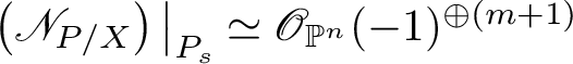
By (the same argument as) [Reference Lee, Lin and Wang35, §1], there exists a vector bundle
 $F^{\prime }$
of rank
$F^{\prime }$
of rank
 $m+1$
such that
$m+1$
such that
 $\mathscr {N}_{P/X} = \mathscr {O}_{\mathbb {P}_{\text {sub}}(F)}(-1) \otimes \psi ^* F^{\prime }$
. If we blow up X along P, we get
$\mathscr {N}_{P/X} = \mathscr {O}_{\mathbb {P}_{\text {sub}}(F)}(-1) \otimes \psi ^* F^{\prime }$
. If we blow up X along P, we get
 $\pi \colon \widetilde {X} \to X$
with exceptional divisor
$\pi \colon \widetilde {X} \to X$
with exceptional divisor
 $E = \mathbb {P}_{\text {sub}}\left (\mathscr {N}_{P/X} \right ) = \mathbb {P}_{S, \text {sub}}(F) \times _S \mathbb {P}_{S, \text {sub}}(F^{\prime })$
. Furthermore, one can blow down E along fibers of
$E = \mathbb {P}_{\text {sub}}\left (\mathscr {N}_{P/X} \right ) = \mathbb {P}_{S, \text {sub}}(F) \times _S \mathbb {P}_{S, \text {sub}}(F^{\prime })$
. Furthermore, one can blow down E along fibers of
 $\mathbb {P}_{S, \text {sub}}(F)$
and get
$\mathbb {P}_{S, \text {sub}}(F)$
and get
 $\pi ^{\prime } \colon \widetilde {X} \to X^{\prime }$
and
$\pi ^{\prime } \colon \widetilde {X} \to X^{\prime }$
and
 $\pi ^{\prime }(E) = :P^{\prime } \simeq \mathbb {P}_{S, \text {sub}}(F^{\prime })$
, with
$\pi ^{\prime }(E) = :P^{\prime } \simeq \mathbb {P}_{S, \text {sub}}(F^{\prime })$
, with
 $\mathscr {N}_{P^{\prime }/X^{\prime }} \simeq \mathscr {O}_{\mathbb {P}_{\text {sub}} (F^{\prime })}(-1) \otimes \psi ^{\prime *} F$
, where
$\mathscr {N}_{P^{\prime }/X^{\prime }} \simeq \mathscr {O}_{\mathbb {P}_{\text {sub}} (F^{\prime })}(-1) \otimes \psi ^{\prime *} F$
, where
 $\psi ^{\prime } \colon P^{\prime } \to S$
is the natural projection. Hence we obtain another log-extremal contraction
$\psi ^{\prime } \colon P^{\prime } \to S$
is the natural projection. Hence we obtain another log-extremal contraction
 $(\Psi ', \psi ^{\prime }):(X^{\prime },P^{\prime }) \to \left (\overline {X}, S\right )$
, which is birational to
$(\Psi ', \psi ^{\prime }):(X^{\prime },P^{\prime }) \to \left (\overline {X}, S\right )$
, which is birational to
 $(X,P)$
.
$(X,P)$
.
The birational map
 $f: X \dashrightarrow X^{\prime }$
is called a standard (or ordinary) flip of type
$f: X \dashrightarrow X^{\prime }$
is called a standard (or ordinary) flip of type
 $(n,m)$
. Note that
$(n,m)$
. Note that
 $X>_{K} X^{\prime }$
(resp.,
$X>_{K} X^{\prime }$
(resp.,
 $X \simeq _K X^{\prime }$
) if and only if
$X \simeq _K X^{\prime }$
) if and only if
 $n>m$
(resp.,
$n>m$
(resp.,
 $n=m$
).
$n=m$
).
The geometry is illustrated in the following diagram, with maps as labeled:

If
 $X>_{K} X^{\prime }$
(resp.,
$X>_{K} X^{\prime }$
(resp.,
 $X \simeq _K X^{\prime }$
), the expected relations of derived categories for the flip (resp., flop)
$X \simeq _K X^{\prime }$
), the expected relations of derived categories for the flip (resp., flop)
 $f\colon X \dashrightarrow X^{\prime }$
are established by Bondal and Orlov [Reference Bernardara, Bolognesi and Faenzi8]. In this section we establish the corresponding relations on Chow groups, which complement the results of [Reference Lee, Lin and Wang35, §3].
$f\colon X \dashrightarrow X^{\prime }$
are established by Bondal and Orlov [Reference Bernardara, Bolognesi and Faenzi8]. In this section we establish the corresponding relations on Chow groups, which complement the results of [Reference Lee, Lin and Wang35, §3].
From now on we assume
 $n \ge m$
– that is,
$n \ge m$
– that is,
 $X \ge _K X^{\prime }$
. Denote
$X \ge _K X^{\prime }$
. Denote
 $\Gamma $
the graph closure of f in
$\Gamma $
the graph closure of f in
 $X^{\prime } \times X$
, which is nothing but
$X^{\prime } \times X$
, which is nothing but
 $\widetilde {X} = X \times _{\overline {X}} X^{\prime }$
. Denote by
$\widetilde {X} = X \times _{\overline {X}} X^{\prime }$
. Denote by
 $\Gamma _*\colon \operatorname {CH}_k(X) \to \operatorname {CH}_k(X^{\prime })$
and
$\Gamma _*\colon \operatorname {CH}_k(X) \to \operatorname {CH}_k(X^{\prime })$
and
 $\Gamma ^* \colon \operatorname {CH}_k(X^{\prime }) \to \operatorname {CH}_k(X)$
the maps induced by
$\Gamma ^* \colon \operatorname {CH}_k(X^{\prime }) \to \operatorname {CH}_k(X)$
the maps induced by
 $[\Gamma ] \in \operatorname {CH}_{\dim X}(X \times X^{\prime })$
. It is easy to see that
$[\Gamma ] \in \operatorname {CH}_{\dim X}(X \times X^{\prime })$
. It is easy to see that
 $$ \begin{align*} \Gamma_*(\underline{\hphantom{A}}) = \pi^{\prime}_* \pi^*(\underline{\hphantom{A}}), \qquad \Gamma^*(\underline{\hphantom{A}}) = \pi_* \pi^{\prime*}(\underline{\hphantom{A}}). \end{align*} $$
Denote by
 $\mathscr {V}$
and
$\mathscr {V}$
and
 $\mathscr {V}^{\prime }$
the respective excess bundles for the blowups
$\mathscr {V}^{\prime }$
the respective excess bundles for the blowups
 $\pi \colon \widetilde {X} \to X$
and
$\pi \colon \widetilde {X} \to X$
and
 $\pi ^{\prime } \colon \widetilde {X} \to X^{\prime }$
– that is, they are defined by the short exact sequences
$\pi ^{\prime } \colon \widetilde {X} \to X^{\prime }$
– that is, they are defined by the short exact sequences
 $$ \begin{align*} 0 \to \mathscr{N}_{E/\widetilde{X}} \to p^*\mathscr{N}_{P/X} \to \mathscr{V} \to 0, \qquad 0 \to \mathscr{N}_{E/\widetilde{X}} \to p^{\prime*}\mathscr{N}_{P^{\prime}/X^{\prime}} \to \mathscr{V}^{\prime} \to 0. \end{align*} $$
Denote by
 $\Phi _* \colon \operatorname {CH}_k(P) \to \operatorname {CH}_k(P^{\prime })$
(resp.,
$\Phi _* \colon \operatorname {CH}_k(P) \to \operatorname {CH}_k(P^{\prime })$
(resp.,
 $\Phi ^* \colon \operatorname {CH}_k(P^{\prime }) \to \operatorname {CH}_k(P)$
) the maps given by the correspondence
$\Phi ^* \colon \operatorname {CH}_k(P^{\prime }) \to \operatorname {CH}_k(P)$
) the maps given by the correspondence
 $c_{m}(\mathscr {V}) \in \operatorname {CH}^{m}(P \times _S P^{\prime })$
(resp.,
$c_{m}(\mathscr {V}) \in \operatorname {CH}^{m}(P \times _S P^{\prime })$
(resp.,
 $c_{n}(\mathscr {V}^{\prime }) \in \operatorname {CH}^{n}(P^{\prime } \times _S P)$
) – that is,
$c_{n}(\mathscr {V}^{\prime }) \in \operatorname {CH}^{n}(P^{\prime } \times _S P)$
) – that is,
 $$ \begin{align*} \Phi_*(\underline{\hphantom{A}}) =p^{\prime}_*(c_{m}(\mathscr{V})\cap p^*(\underline{\hphantom{A}})) \qquad \Phi^*(\underline{\hphantom{A}}) = p_*(c_{n}(\mathscr{V}^{\prime})\cap p^{\prime*}(\underline{\hphantom{A}})). \end{align*} $$
It follows from the Euler sequence that
 $\mathscr {V} = \mathscr {O}_{P}(-1) \boxtimes \mathcal {T}_{P^{\prime }/S}(-1)$
and
$\mathscr {V} = \mathscr {O}_{P}(-1) \boxtimes \mathcal {T}_{P^{\prime }/S}(-1)$
and
 $\mathscr {V}^{\prime } = \mathcal {T}_{P/S}(-1) \boxtimes \mathscr {O}_{P^{\prime }}(-1)$
.
$\mathscr {V}^{\prime } = \mathcal {T}_{P/S}(-1) \boxtimes \mathscr {O}_{P^{\prime }}(-1)$
.
Theorem 3.6 standard flips
Let
 $f: X \dashrightarrow X^{\prime }$
be a standard flip and assume
$f: X \dashrightarrow X^{\prime }$
be a standard flip and assume
 $X^{\prime }$
is nonsingular and quasi-projective. Then we have the following:
$X^{\prime }$
is nonsingular and quasi-projective. Then we have the following:
-
(1) The following holds:
$$ \begin{align*} \Gamma_* \Gamma^* = \operatorname{Id}_{\operatorname{CH}(X^{\prime})}, \qquad \Phi_* \Phi^* = \operatorname{Id}_{\operatorname{CH}(P^{\prime})}. \end{align*} $$
-
(2) There exists a split short exact sequence
where a left inverse of the first map is given by
$$ \begin{align*} 0 \to \operatorname{CH}_{k}(P^{\prime}) \xrightarrow{\left(\Phi^*, -i^{\prime}_*\right)} \operatorname{CH}_{k}(P) \oplus \operatorname{CH}_{k}(X^{\prime}) \xrightarrow{\left(\gamma, \alpha^{\prime}\right)\mapsto i_*\gamma + \Gamma^* \alpha^{\prime}} \operatorname{CH}_k(X) \to 0, \end{align*} $$
$(\gamma , \alpha ^{\prime })\mapsto \Phi _* \gamma $
.
-
(3) This exact sequence induces an isomorphism of Chow groups
(3.6)given by
$$ \begin{align} \operatorname{CH}_{k}(X^{\prime}) \oplus \bigoplus_{i=0}^{n-m-1} \operatorname{CH}_{k-n+i}(S) \xrightarrow{\sim} \operatorname{CH}_{k}(X), \end{align} $$
$\left (\alpha ^{\prime }, \oplus _{i=0}^{n-m-1} \beta _i\right ) \mapsto \Gamma ^* \alpha ^{\prime } + i_*\left (\sum _{i=0}^{n-m-1} \zeta ^i \cdot \psi ^*\beta _i\right )$
. Furthermore, in this decomposition, the projection to the first summand is given by
$\alpha \mapsto \alpha ^{\prime } = \Gamma _* \alpha $
.


Notice that in the flop case
 $m=n$
, this result recovers the invariance of Chow groups under flops in [Reference Lee, Lin and Wang35]; and in the flip case
$m=n$
, this result recovers the invariance of Chow groups under flops in [Reference Lee, Lin and Wang35]; and in the flip case
 $m<n$
, this theorem completes the discussion of [Reference Lee, Lin and Wang35, §2.3] by providing the complementary summands of the image of
$m<n$
, this theorem completes the discussion of [Reference Lee, Lin and Wang35, §2.3] by providing the complementary summands of the image of
 $\Gamma ^*$
in the Chow group
$\Gamma ^*$
in the Chow group
 $\operatorname {CH}(X)$
. Finally, as a blowup can be viewed as a standard flip of type
$\operatorname {CH}(X)$
. Finally, as a blowup can be viewed as a standard flip of type
 $(n,0)$
, the theorem recovers the blowup formula in Theorem 2.8.
$(n,0)$
, the theorem recovers the blowup formula in Theorem 2.8.
Proof of the first part of Theorem 3.6(1). The equality
 $\Gamma _* \Gamma ^* = \operatorname {Id}$
follows exactly the same line of proof as [Reference Lee, Lin and Wang35, Theorem 2.1], as already mentioned in [Reference Lee, Lin and Wang35, §2.3]. We sketch the proof here for completeness. For any class
$\Gamma _* \Gamma ^* = \operatorname {Id}$
follows exactly the same line of proof as [Reference Lee, Lin and Wang35, Theorem 2.1], as already mentioned in [Reference Lee, Lin and Wang35, §2.3]. We sketch the proof here for completeness. For any class
 $[W^{\prime }] \in \operatorname {CH}_k(X^{\prime })$
, by Chow’s moving lemma (if allowing negative coefficients), we may assume it is represented by a cycle
$[W^{\prime }] \in \operatorname {CH}_k(X^{\prime })$
, by Chow’s moving lemma (if allowing negative coefficients), we may assume it is represented by a cycle
 $W^{\prime }$
which intersects
$W^{\prime }$
which intersects
 $P^{\prime }$
transversely. Therefore
$P^{\prime }$
transversely. Therefore
 $\pi ^{\prime *}[W^{\prime }] = \left [\widetilde {W}\right ]$
by [Reference Fulton18, Corollary 6.7.2], where
$\pi ^{\prime *}[W^{\prime }] = \left [\widetilde {W}\right ]$
by [Reference Fulton18, Corollary 6.7.2], where
 $\widetilde {W}$
is the blowup of
$\widetilde {W}$
is the blowup of
 $W^{\prime }$
along
$W^{\prime }$
along
 $W^{\prime } \cap P^{\prime }$
. Hence
$W^{\prime } \cap P^{\prime }$
. Hence
 $\Gamma ^*[W^{\prime }] = \pi _* \left [\widetilde {W}\right ] = [W]$
, where W is the image of
$\Gamma ^*[W^{\prime }] = \pi _* \left [\widetilde {W}\right ] = [W]$
, where W is the image of
 $\widetilde {W}$
and is also the proper transform of
$\widetilde {W}$
and is also the proper transform of
 $W^{\prime }$
along the birational rational map
$W^{\prime }$
along the birational rational map
 $f^{-1}$
. Now we have
$f^{-1}$
. Now we have
 $$ \begin{align*} \pi^* [W] = \left[\widetilde{W}\right] + j_* \sum_{B} [E_{B}], \end{align*} $$
where we let
 $B^{\prime } \subset W^{\prime } \cap P^{\prime }$
be a component; then
$B^{\prime } \subset W^{\prime } \cap P^{\prime }$
be a component; then
 $E_{B} \subset E$
are k-cycles supported over components
$E_{B} \subset E$
are k-cycles supported over components
 $\overline {B} = \psi ^{\prime }(B^{\prime }) \subset \psi ^{\prime }(W^{\prime } \cap P^{\prime }) \subset S$
. A direct computation of dimensions shows that for a general point s, the fiber
$\overline {B} = \psi ^{\prime }(B^{\prime }) \subset \psi ^{\prime }(W^{\prime } \cap P^{\prime }) \subset S$
. A direct computation of dimensions shows that for a general point s, the fiber
 $E_{B,s}$
over s has dimension
$E_{B,s}$
over s has dimension
 $$ \begin{align*} \dim E_{B,s} \ge \dim E_{B} - \dim \left(\overline{B}\right) \ge \dim E_{B} - \dim ({B^{\prime}}) = k - (k - (n+1)) = n+1. \end{align*} $$
Now
 $E_{B,s}$
must contain positive fibers of of
$E_{B,s}$
must contain positive fibers of of
 $p^{\prime }_s \colon \mathbb {P}_s^n \times \mathbb {P}_s^m \to \mathbb {P}_s^m$
, as
$p^{\prime }_s \colon \mathbb {P}_s^n \times \mathbb {P}_s^m \to \mathbb {P}_s^m$
, as
 $n+1> n \ge m$
. Hence
$n+1> n \ge m$
. Hence
 $\pi _* j_*[E_B] = p_*[E_B] = 0$
, and
$\pi _* j_*[E_B] = p_*[E_B] = 0$
, and
 $\Gamma _* \Gamma ^* [W^{\prime }] = \pi ^{\prime }_* \pi ^* [W] =\pi ^{\prime }_* \left [\widetilde {W}\right ] = [W^{\prime }]$
.□
$\Gamma _* \Gamma ^* [W^{\prime }] = \pi ^{\prime }_* \pi ^* [W] =\pi ^{\prime }_* \left [\widetilde {W}\right ] = [W^{\prime }]$
.□
Remark 3.7. Notice that this argument does not work in the other direction for
 $\Gamma ^* \Gamma _* [V]$
, where
$\Gamma ^* \Gamma _* [V]$
, where
 $[V] \in \operatorname {CH}_k(X)$
. The reason is as follows: the fiber
$[V] \in \operatorname {CH}_k(X)$
. The reason is as follows: the fiber
 $E_{B^{\prime },s}$
of the k-cycle
$E_{B^{\prime },s}$
of the k-cycle
 $E_{B^{\prime }}$
in
$E_{B^{\prime }}$
in
 $\pi ^{\prime *}\Gamma ^* [V] = \pi ^{\prime *}[V'] = \widetilde {V} + j_* \sum E_{B^{\prime }}$
has dimension
$\pi ^{\prime *}\Gamma ^* [V] = \pi ^{\prime *}[V'] = \widetilde {V} + j_* \sum E_{B^{\prime }}$
has dimension
 $\ge m+1$
, but
$\ge m+1$
, but
 $m \le n$
, and thus
$m \le n$
, and thus
 $E_{B^{\prime },s}$
is not necessarily contracted by
$E_{B^{\prime },s}$
is not necessarily contracted by
 $p_*$
. However, if
$p_*$
. However, if
 $k \le m$
(in which case we may assume
$k \le m$
(in which case we may assume
 $V \cap P = \emptyset $
) or
$V \cap P = \emptyset $
) or
 $k \ge n+1 + \dim \psi (V \cap S)$
– for example, if
$k \ge n+1 + \dim \psi (V \cap S)$
– for example, if
 $k \ge \dim S + n +1$
– then the argument still works:
$k \ge \dim S + n +1$
– then the argument still works:
 $$ \begin{align*} \Gamma^* \Gamma_* [V] = [V] \qquad \text{if } k \le m+1 \text{ or } k \ge n + \dim \psi(V \cap S). \end{align*} $$
For the intermediate cases
 $m+1\le k \le n + \dim \psi (V \cap S) \le n + \dim S$
, the same argument implies only
$m+1\le k \le n + \dim \psi (V \cap S) \le n + \dim S$
, the same argument implies only
 $\Gamma ^* \Gamma _* [V] = [V] + i_* \sum _{Z \subset P} [Z]$
for certain cycles
$\Gamma ^* \Gamma _* [V] = [V] + i_* \sum _{Z \subset P} [Z]$
for certain cycles
 $Z \subset P$
supported on P; these cycles will be precisely explained by statements (2) and (3) of the theorem.
$Z \subset P$
supported on P; these cycles will be precisely explained by statements (2) and (3) of the theorem.
Proof of the second part of Theorem 3.6(1). It follows from Lemma 2.7 that
 $$ \begin{align*} c_{m}(\mathscr{V}) &= (-1)^m c_m\left(\mathscr{O}_{P}(1) \boxtimes \Omega_{P^{\prime}/S}(1)\right) = (-1)^m \sum_{t=0}^{m} \zeta^t \cdot c_{m-t}\left(\Omega_{P^{\prime}/S}(1)\right)\\[-3pt] &= (-1)^m \sum_{t=0}^{m} (-1)^{m-t} \sum_{s=0}^{m-t} c_{s}(F^{\prime}) \cdot (\zeta')^{m-s-t} \cdot \zeta^t \end{align*} $$
and
 $$ \begin{align*} c_{n}(\mathscr{V}^{\prime}) &= (-1)^n c_n\left(\Omega_{P/S}(1)\boxtimes \mathscr{O}_{P^{\prime}}(1) \right ) = (-1)^n \sum_{j=0}^{n} c_{n-j}\left(\Omega_{P/S}(1)\right)\cdot (\zeta^{\prime})^j \\[-3pt] &= (-1)^n \sum_{j=0}^{n} (-1)^{n-j} \sum_{i=0}^{n-j} c_{i}(F) \cdot \zeta^{n-i-j} \cdot (\zeta^{\prime})^{j}. \end{align*} $$
The map
 $\Phi _* \circ \Phi ^*$
is given by the convolution of correspondences
$\Phi _* \circ \Phi ^*$
is given by the convolution of correspondences
 $$ \begin{align*} c_{m}(\mathscr{V}) *c_{n}(\mathscr{V}^{\prime}) := p_{13*}\left(p_{12}^*(c_{n}(\mathscr{V}^{\prime})) \cdot p_{23}^* (c_{m}(\mathscr{V})) \right) \in \operatorname{CH}^{m}(P^{\prime} \times_S P^{\prime}), \end{align*} $$
where
 $p_{ij}$
are the obvious projections from
$p_{ij}$
are the obvious projections from
 $P^{\prime } \times _S P \times _S P^{\prime }$
to the corresponding factors and the cohomological degree m is computed via
$P^{\prime } \times _S P \times _S P^{\prime }$
to the corresponding factors and the cohomological degree m is computed via
 $m+n -\dim (P/S) = m$
. To avoid confusion, we denote the product
$m+n -\dim (P/S) = m$
. To avoid confusion, we denote the product
 $P^{\prime } \times _S P \times _S P^{\prime }$
by
$P^{\prime } \times _S P \times _S P^{\prime }$
by
 $P_1' \times _S P \times _S P_2'$
, and denote the relative
$P_1' \times _S P \times _S P_2'$
, and denote the relative
 $\mathscr {O}(1)$
-classes of
$\mathscr {O}(1)$
-classes of
 $P_1'$
and
$P_1'$
and
 $P_2'$
by
$P_2'$
by
 $\zeta ^{\prime }_1$
and
$\zeta ^{\prime }_1$
and
 $\zeta ^{\prime }_2$
, respectively. Therefore,
$\zeta ^{\prime }_2$
, respectively. Therefore,
 $$ \begin{align*} c_{m}(\mathscr{V}) *c_{n}(\mathscr{V}^{\prime}) = p_{13*}\!\left(\!\sum_{j=0}^{n} \sum_{t=0}^{m}\! (-1)^{j+t} \!\sum_{s=0}^{m-t} \sum_{i=0}^{n-j}\! c_{s}\!\left(F_2'\right) \cdot c_{i}(F) \cdot \zeta^{n+t-i-j} \cdot\!\left(\zeta_1'\right)^{j} \cdot \!\left(\zeta_2'\right)^{m-s-t} \!\right)\!. \end{align*} $$
Since
 $p_{13*}(\zeta ^k) = 0$
for all
$p_{13*}(\zeta ^k) = 0$
for all
 $0 \le k \le n-1$
, the only terms inside the parentheses that could survive
$0 \le k \le n-1$
, the only terms inside the parentheses that could survive
 $p_{13*}$
are the ones whose indices satisfy
$p_{13*}$
are the ones whose indices satisfy
 $t-i-j \ge 0$
. Thus we may assume that the indices of the summation satisfy
$t-i-j \ge 0$
. Thus we may assume that the indices of the summation satisfy
 $j \le t \le m$
and
$j \le t \le m$
and
 $0 \le i \le t-j$
. From the definition of the Segre class of F, we have
$0 \le i \le t-j$
. From the definition of the Segre class of F, we have
 $p_{13*}\left (\zeta ^{n+k}\right ) = s_k(F)$
, hence
$p_{13*}\left (\zeta ^{n+k}\right ) = s_k(F)$
, hence
 $$ \begin{align*} c_{m}(\mathscr{V}) *c_{n}(\mathscr{V}^{\prime}) = \sum_{j=0}^{m} \sum_{t=j}^{m} (-1)^{j+t} \sum_{s=0}^{m-t} \sum_{i=0}^{t-j} c_{i}(F) \cdot s_{t-i-j}(F) \cdot c_{s}\left(F_2'\right) \cdot\left(\zeta_1'\right)^{j} \cdot \left(\zeta_2'\right)^{m-s-t}. \end{align*} $$
From
 $c(F) s(F) = 1$
, we know that
$c(F) s(F) = 1$
, we know that
 $\sum _{i=0}^{t-j} c_{i}(F) \cdot s_{t-i-j}(F) = 0$
unless
$\sum _{i=0}^{t-j} c_{i}(F) \cdot s_{t-i-j}(F) = 0$
unless
 $t=j$
, in which case
$t=j$
, in which case
 $c_0(F) s_0(F) =1$
. Hence this expression reduces to
$c_0(F) s_0(F) =1$
. Hence this expression reduces to
 $$ \begin{align*} c_{m}(\mathscr{V}) *c_{n}(\mathscr{V}^{\prime}) &= \sum_{j=0}^{m} \sum_{s=0}^{m-j} c_{s}\left(F_2'\right) \cdot\left(\zeta_1'\right)^{j} \cdot \left(\zeta_2'\right)^{m-j-s} = \sum_{j=0}^{m} c_{m-j}\left(\mathcal{T}_{P_2'/S}(-1)\right) \cdot\left(\zeta_1'\right)^{j} \\ & = c_m \left(\mathscr{O}_{P_1'}(1) \boxtimes \mathcal{T}_{P_2'/S}(-1)\right). \end{align*} $$
(For the second equality, we used Lemma 2.7.) On the other hand, the diagonal
 $\Delta _{P^{\prime }} \subset P^{\prime } \times _S P^{\prime }$
is the zero locus of a regular section s of the rank m vector bundle
$\Delta _{P^{\prime }} \subset P^{\prime } \times _S P^{\prime }$
is the zero locus of a regular section s of the rank m vector bundle
 $\mathscr {O}_{P^{\prime }}(1) \boxtimes \mathcal {T}_{P^{\prime }/S}(-1)$
; the section s under the canonical identification
$\mathscr {O}_{P^{\prime }}(1) \boxtimes \mathcal {T}_{P^{\prime }/S}(-1)$
; the section s under the canonical identification
 $$ \begin{align*} \Gamma\left(P^{\prime} \times_S P^{\prime}, \mathscr{O}_{P^{\prime}}(1) \boxtimes \mathcal{T}_{P^{\prime}/S}(-1)\right) = \Gamma\left(S, F^{\prime\vee} \otimes F^{\prime}\right) = \operatorname{Hom}_S(F^{\prime},F^{\prime}) \end{align*} $$
corresponds to
 $1_{F^{\prime }} \colon F^{\prime } \to F^{\prime }$
. Hence
$1_{F^{\prime }} \colon F^{\prime } \to F^{\prime }$
. Hence
 $ [\Delta _{P^{\prime }}] = c_m\left (\mathscr {O}_{P^{\prime }}(1) \boxtimes \mathcal {T}_{P^{\prime }/S}(-1)\right )$
, and therefore
$ [\Delta _{P^{\prime }}] = c_m\left (\mathscr {O}_{P^{\prime }}(1) \boxtimes \mathcal {T}_{P^{\prime }/S}(-1)\right )$
, and therefore
 $$ \begin{align*} c_{m}(\mathscr{V}) *c_{n}(\mathscr{V}^{\prime}) = [\Delta_{P^{\prime}}], \qquad \text{hence } \Phi_* \, \Phi^* = \operatorname{Id}_{\operatorname{CH}(P^{\prime})}. \\[-36pt]\end{align*} $$
□
Before proceeding the rest of the proof of Theorem 3.6, we study more about the maps
 $\Phi _*$
and
$\Phi _*$
and
 $\Phi ^*$
. First, notice that the projective bundle formula (Theorem 2.4) can be regarded as equipping
$\Phi ^*$
. First, notice that the projective bundle formula (Theorem 2.4) can be regarded as equipping
 $\operatorname {CH}(P)$
and
$\operatorname {CH}(P)$
and
 $\operatorname {CH}(P^{\prime })$
with natural ‘free module structures over
$\operatorname {CH}(P^{\prime })$
with natural ‘free module structures over
 $\operatorname {CH}(S)$
’:
$\operatorname {CH}(S)$
’:
Lemma 3.8.
-
(1) The maps
$\Phi _* \colon \operatorname {CH}(P) \to \operatorname {CH}(P^{\prime })$
and
$\Phi ^* \colon \operatorname {CH}(P^{\prime }) \to \operatorname {CH}(P)$
are ‘
$\operatorname {CH}(S)$
-linear’ – that is, for all
$\alpha \in \operatorname {CH}^*(P)$
,
$\alpha ^{\prime } \in \operatorname {CH}^*(P^{\prime })$
, and
$\theta \in \operatorname {CH}_*(S)$
,
$$ \begin{align*} \Phi_*(\alpha \cap \psi^* \theta) = \Phi_*(\alpha) \cap \psi^{\prime*} \theta, \qquad \Phi^*(\alpha^{\prime} \cap \psi^{\prime*} \theta) = \Phi^*(\alpha^{\prime}) \cap \psi^* \theta. \end{align*} $$
-
(2) Consider the following ‘sub-
$\operatorname {CH}(S)$
-modules’ of
$ \operatorname {CH}(P)$
: Then
$$ \begin{align*} & \operatorname{CH}(P)_{m} : = \operatorname{Span}\left\{\zeta^{n-m}, \zeta^{n-m+1}, \dotsc, \zeta^{m} \right\}\\ &\qquad\qquad = \zeta^{n-m} \cdot \operatorname{CH}(S) \oplus \dotsb \oplus \zeta^{m} \cdot \operatorname{CH}(S) \subset \operatorname{CH}(P), \\ & \operatorname{CH}(P)_{\Phi_*=0} {\,: =\,} \operatorname{Span} \left\{ 1, \zeta, \dotsc, \zeta^{n-m-1} \right\} {\,=\,} 1 \cdot \operatorname{CH}(S) \oplus \dotsb \oplus \zeta^{n-m-1} \cdot \operatorname{CH}(S) \subset \operatorname{CH}(P). \end{align*} $$
$\Phi _*$
is injective on
$\operatorname {CH}(P)_{m}$
, and with image
$\Phi _*(\operatorname {CH}(P)_{m}) = \operatorname {CH}(P^{\prime })$
. Furthermore,
$\Phi _*$
is zero on
$\operatorname {CH}(P)_{\Phi _*=0}$
.
-
(3)
$\Phi ^*$
is injective, and its image
$\operatorname {Im}(\Phi ^*)$
satisfies
$\operatorname {CH}(P)_{\Phi _*=0} \simeq \operatorname {CH}(P)/\operatorname {Im}(\Phi ^*)$
.


Proof. Statement (1) follows directly from the projection formula [Reference Fulton18, Theorem 3.2(c)] and Theorem 2.4(1). For statement (2), notice that for any
 $0 \le i \le m$
,
$0 \le i \le m$
,
 $$ \begin{align*} \Phi_* \left(\zeta^{n-m+i}\right)& = p^{\prime}_* \left(c_{m}(\mathscr{V}) \cup p^*\zeta^{n-m+i}\right) \\ &= p^{\prime}_*\left((-1)^m \sum_{t=0}^{m} (-1)^{m-t} \sum_{s=0}^{m-t} c_{s}(F^{\prime}) \cdot (\zeta^{\prime})^{m-s-t} \cdot \zeta^{n-m+i+t}\right) \\ & = \sum_{t=m-i}^{m} (-1)^{t} \sum_{s=0}^{m-t} c_{s}(F^{\prime}) \cdot s_{t-(m-i)}(F) \cdot (\zeta^{\prime})^{m-s-t} \\ & = (-1)^{m-i} (\zeta^{\prime})^{i} + (\text{lower-order terms}). \end{align*} $$
(For example,
 $\Phi _* (\zeta ^m) = (\zeta ^{\prime })^{n} + (\text {lower-order terms})$
and
$\Phi _* (\zeta ^m) = (\zeta ^{\prime })^{n} + (\text {lower-order terms})$
and
 $\Phi _* (\zeta ^n) = (-1)^n (\zeta ^{\prime })^{0}$
.) This computation together with statement (1) shows that
$\Phi _* (\zeta ^n) = (-1)^n (\zeta ^{\prime })^{0}$
.) This computation together with statement (1) shows that
 $\Phi _* \left (\zeta ^{n-m+i} \cap \psi ^* \theta \right ) = \left (\pm \zeta ^{\prime i} + (\text {lower-order terms})\right ) \cap \psi ^{\prime *} \theta $
for all
$\Phi _* \left (\zeta ^{n-m+i} \cap \psi ^* \theta \right ) = \left (\pm \zeta ^{\prime i} + (\text {lower-order terms})\right ) \cap \psi ^{\prime *} \theta $
for all
 $\theta \in \operatorname {CH}(S)$
, which implies the injectivity of
$\theta \in \operatorname {CH}(S)$
, which implies the injectivity of
 $\Phi _*$
on
$\Phi _*$
on
 $\operatorname {CH}(P)_{m}$
. The same computation in the case
$\operatorname {CH}(P)_{m}$
. The same computation in the case
 $i<0$
shows that
$i<0$
shows that
 $\Phi _*$
is zero on
$\Phi _*$
is zero on
 $\operatorname {CH}(P)_{\Phi _*=0}$
. A similar computation shows
$\operatorname {CH}(P)_{\Phi _*=0}$
. A similar computation shows
 $$ \begin{align*} \Phi^*\left(\zeta^{\prime i}\right) = \pm \zeta^{n-m+i} + (\text{lower-order terms}) \end{align*} $$
for
 $0 \le i \le m$
, which implies statement (3).
$0 \le i \le m$
, which implies statement (3).
Lemma 3.9. For any
 $\gamma \in \operatorname {CH}(P)$
, if
$\gamma \in \operatorname {CH}(P)$
, if
 $\Phi _*(\gamma ) = 0$
and
$\Phi _*(\gamma ) = 0$
and
 $i^* i_* \gamma =0$
, then
$i^* i_* \gamma =0$
, then
 $\gamma =0$
.
$\gamma =0$
.
Proof. Let
 $\gamma = \sum _{i=0}^{n} \zeta ^i \cdot \psi ^* \theta _i$
for
$\gamma = \sum _{i=0}^{n} \zeta ^i \cdot \psi ^* \theta _i$
for
 $\theta _i \in \operatorname {CH}(S)$
. Then from the lemma,
$\theta _i \in \operatorname {CH}(S)$
. Then from the lemma,
 $\Phi _* \gamma = 0$
implies
$\Phi _* \gamma = 0$
implies
 $\theta _{n-m} = \theta _{n-m+1} = \dotsb = \theta _{n} = 0$
. On the other hand,
$\theta _{n-m} = \theta _{n-m+1} = \dotsb = \theta _{n} = 0$
. On the other hand,
 $i^* i_* \gamma = c_{m+1}\left (\mathscr {N}_{P/X}\right ) \cap \gamma = c_{m+1}(F^{\prime }\otimes \mathscr {O}_P(-1)) \cap \gamma = 0$
, and
$i^* i_* \gamma = c_{m+1}\left (\mathscr {N}_{P/X}\right ) \cap \gamma = c_{m+1}(F^{\prime }\otimes \mathscr {O}_P(-1)) \cap \gamma = 0$
, and
 $$ \begin{align*} c_{m+1}(F^{\prime}\otimes \mathscr{O}_P(-1)) & = \sum_{i=0}^{m+1} c_{m+1-i}(F^{\prime}) (-\zeta)^i \\ &= (-1)^{m+1} \zeta^{m+1} + (\text{lower-order terms}). \end{align*} $$
Hence by the uniqueness of an expression of the form
 $\sum _{i=0}^{n} \zeta ^i \cdot \psi ^*(\underline {\hphantom {A}})$
, one can inductively show
$\sum _{i=0}^{n} \zeta ^i \cdot \psi ^*(\underline {\hphantom {A}})$
, one can inductively show
 $\theta _{n-m-1} = 0, \theta _{n-m-2} = 0, \dotsc , \theta _0 = 0$
. Therefore
$\theta _{n-m-1} = 0, \theta _{n-m-2} = 0, \dotsc , \theta _0 = 0$
. Therefore
 $\gamma =0$
.
$\gamma =0$
.
Proof of Theorem 3.6(2). To show that the sequence is a complex, simply observe that for any
 $\gamma ^{\prime } \in \operatorname {CH}(P)$
,
$\gamma ^{\prime } \in \operatorname {CH}(P)$
,
 $$ \begin{align*} i_*\Phi^*\gamma^{\prime} + \Gamma^*\left(-i^{\prime}_* \gamma^{\prime}\right) &= i_*p_*(c_n(\mathscr{V}^{\prime})\cap p^{\prime*}\gamma^{\prime}) - \Gamma^*\,i^{\prime}_*\, \gamma^{\prime} \\ &= \pi_*j_*(c_n(\mathscr{V}^{\prime})\cap p^{\prime*}\gamma^{\prime}) - \Gamma^*i^{\prime}_* \gamma^{\prime} \\ & \overset{\text{(k.f.)}}{=} \pi_*\pi^{\prime*}i^{\prime}_* \gamma^{\prime} - \pi_*\pi^{\prime*}i^{\prime}_* \gamma^{\prime} = 0. \end{align*} $$
(Here and later, ‘(k.f.)’ means the key formula (2.2) for blowup.)
For any
 $\alpha \in \operatorname {CH}_k(X)$
,
$\alpha \in \operatorname {CH}_k(X)$
,
 $\alpha - \Gamma ^* \Gamma _* \alpha = 0$
on
$\alpha - \Gamma ^* \Gamma _* \alpha = 0$
on
 $\operatorname {CH}_k(X \backslash P)$
. Then from the exact sequence
$\operatorname {CH}_k(X \backslash P)$
. Then from the exact sequence
 $\operatorname {CH}_k(P) \to \operatorname {CH}_k(X) \to \operatorname {CH}_k(X\backslash P) \to 0$
, there exists an element
$\operatorname {CH}_k(P) \to \operatorname {CH}_k(X) \to \operatorname {CH}_k(X\backslash P) \to 0$
, there exists an element
 $\gamma \in \operatorname {CH}_k(P)$
such that
$\gamma \in \operatorname {CH}_k(P)$
such that
 $\alpha = \Gamma ^* \Gamma _* \alpha + i_* \gamma $
. This establishes the surjectivity of the last map of the sequence of Theorem 3.6(2). The injectivity of the first map and the left inverse statement follow directly from
$\alpha = \Gamma ^* \Gamma _* \alpha + i_* \gamma $
. This establishes the surjectivity of the last map of the sequence of Theorem 3.6(2). The injectivity of the first map and the left inverse statement follow directly from
 $\Phi _* \Phi _* = \operatorname {Id}$
. To show that the sequence is exactness in the middle, assume
$\Phi _* \Phi _* = \operatorname {Id}$
. To show that the sequence is exactness in the middle, assume
 $(\gamma , \alpha ^{\prime }) \in \operatorname {CH}(P)\oplus \operatorname {CH}(X^{\prime })$
such that
$(\gamma , \alpha ^{\prime }) \in \operatorname {CH}(P)\oplus \operatorname {CH}(X^{\prime })$
such that
 $i_*\gamma + \Gamma ^* \alpha ^{\prime }=0$
; we want to find
$i_*\gamma + \Gamma ^* \alpha ^{\prime }=0$
; we want to find
 $\gamma ^{\prime }$
such that
$\gamma ^{\prime }$
such that
 $(\gamma , \alpha ^{\prime }) = \left (\Phi ^* \gamma ^{\prime }, -i^{\prime }_* \gamma \right )$
, since
$(\gamma , \alpha ^{\prime }) = \left (\Phi ^* \gamma ^{\prime }, -i^{\prime }_* \gamma \right )$
, since
 $$ \begin{align*} \alpha^{\prime} & = \Gamma_* \Gamma^* \alpha^{\prime} = - \Gamma_* i_* \gamma = - \pi^{\prime}_* \pi^* i_* \gamma \overset{\text{(k.f.)}}{=} -\pi^{\prime}_* j_* (c_{m}(\mathscr{V}) \cap p^*\gamma) \\ & = -i^{\prime}_* p^{\prime}_*(c_{m}(\mathscr{V}) \cap p^* \gamma) = -i^{\prime}_* \Phi_* (\gamma). \end{align*} $$
Define
 $\gamma _0 = \gamma - \Phi ^* \Phi _* \gamma .$
The goal is to show
$\gamma _0 = \gamma - \Phi ^* \Phi _* \gamma .$
The goal is to show
 $\gamma _0 =0$
. Notice that
$\gamma _0 =0$
. Notice that
 $$ \begin{align*} \Phi_* \gamma_0 &= \Phi_* \gamma - \Phi_* \Phi^* \Phi_* \gamma = 0 \end{align*} $$
and
 $$ \begin{align*} i_*\gamma_0 & = i_* \gamma - i_* \Phi^* \Phi_* \gamma = i_* \gamma - i_* p_* (c_n{\mathscr{V}^{\prime}} \cap p^{\prime*} (\Phi^* \gamma)) \\ & = i_* \gamma - \pi_* j_*(c_n{\mathscr{V}^{\prime}} \cap p^{\prime*} ( \Phi_* \gamma)) \overset{\text{(k.f.)}}{=} i_* \gamma - \pi_* \pi^{\prime*} i^{\prime}_* \Phi_* \gamma \\ & = i_* \gamma - \Gamma^* \left(i^{\prime}_* \Phi_* \gamma\right) = i_* \gamma + \Gamma^* \alpha^{\prime} = 0. \end{align*} $$
From Lemma 3.9,
 $\gamma _0 = 0$
, hence
$\gamma _0 = 0$
, hence
 $(\gamma , \alpha ^{\prime }) = \left (\Phi ^* \gamma ^{\prime }, -i^{\prime }_* \gamma \right )$
for
$(\gamma , \alpha ^{\prime }) = \left (\Phi ^* \gamma ^{\prime }, -i^{\prime }_* \gamma \right )$
for
 $\gamma ^{\prime } = \Phi _* \, \gamma $
.□
$\gamma ^{\prime } = \Phi _* \, \gamma $
.□
Proof of Theorem 3.6(3). As before, from Lemma 3.8(3) and the exact sequence of part (2), we obtain that for any
 $\alpha \in \operatorname {CH}_{k}(X)$
, there exist an
$\alpha \in \operatorname {CH}_{k}(X)$
, there exist an
 $\alpha ^{\prime } \in \operatorname {CH}_{k}(X)$
and a unique
$\alpha ^{\prime } \in \operatorname {CH}_{k}(X)$
and a unique
 $\gamma \in \operatorname {CH}_k(P)$
such that
$\gamma \in \operatorname {CH}_k(P)$
such that
 $\Phi _* \gamma = 0$
and
$\Phi _* \gamma = 0$
and
 $\alpha = \Gamma ^* \alpha ^{\prime } + i_* \gamma $
. Further notice that
$\alpha = \Gamma ^* \alpha ^{\prime } + i_* \gamma $
. Further notice that
 $$ \begin{align*} \Gamma_* i_* \gamma = \pi^{\prime}_*\pi^*i_*\gamma \overset{\text{(k.f.)}}{=} \pi^{\prime}_*j_*(c_n(\mathscr{V}) \cap p^*\gamma) = i^{\prime}_*p^{\prime}_* j_*(c_n(\mathscr{V}) \cap p^*\gamma) = i^{\prime}_* \Phi_* \gamma = 0. \\[-15pt]\end{align*} $$
Therefore
 $\alpha ^{\prime } = \Gamma _* \alpha $
. Hence we have established
$\alpha ^{\prime } = \Gamma _* \alpha $
. Hence we have established
 $$ \begin{align*} \operatorname{CH}_{k}(X) &= \Gamma^* \operatorname{CH}_{k}(X^{\prime}) \oplus i_* \left(\operatorname{CH}(P)_{\Phi_* = 0}\right) \\ & = \Gamma^* \operatorname{CH}_{k}(X^{\prime}) \oplus i_*\left(\bigoplus_{i=0}^{n-m-1} \zeta^i \cdot \psi^* \operatorname{CH}_{k-n+i}(S)\right), \\[-16pt]\end{align*} $$
and the projection to the first summand is given by
 $\alpha \mapsto \alpha ^{\prime } = \Gamma _* \alpha $
.□
$\alpha \mapsto \alpha ^{\prime } = \Gamma _* \alpha $
.□
We could also write down explicitly the projectors to the last
 $(n-m)$
summands; we omit the details here, as we will not need them. As before, by Manin’s identity principle we have the following:
$(n-m)$
summands; we omit the details here, as we will not need them. As before, by Manin’s identity principle we have the following:
Corollary 3.10. If X and
 $X^{\prime }$
are smooth and projective over some ground field
$X^{\prime }$
are smooth and projective over some ground field
 $\Bbbk $
, then there is an isomorphism of Chow motives over
$\Bbbk $
, then there is an isomorphism of Chow motives over
 $\Bbbk $
:
$\Bbbk $
:
 $$ \begin{align*} [\Gamma]^t \oplus \left( \bigoplus_{i=m+1}^n i_* \circ h^{n-i} \circ \psi^* \right) \colon \mathfrak{h}(X^{\prime}) \oplus \left( \bigoplus_{i=m+1}^{n} \mathfrak{h}(S)(i) \right) \xrightarrow{\sim} \mathfrak{h}(X). \\[-15pt]\end{align*} $$
As before, the blowup formula for Chow motives of [Reference Manin39] could be viewed as the case
 $m=0$
of this corollary, as a blowup can be viewed as a standard flip of type
$m=0$
of this corollary, as a blowup can be viewed as a standard flip of type
 $(n,0)$
.
$(n,0)$
.
4 Main results
Let
 $\mathscr {G}$
be a coherent sheaf of homological dimension
$\mathscr {G}$
be a coherent sheaf of homological dimension
 $\le 1$
on X– that is, X is covered by open subschemes
$\le 1$
on X– that is, X is covered by open subschemes
 $U \subset X$
over which there is a resolution
$U \subset X$
over which there is a resolution
 $\mathscr {F} \xrightarrow {~\sigma ~} \mathscr {E} \twoheadrightarrow \mathscr {G}$
such that
$\mathscr {F} \xrightarrow {~\sigma ~} \mathscr {E} \twoheadrightarrow \mathscr {G}$
such that
 $\mathscr {F}$
and
$\mathscr {F}$
and
 $\mathscr {E}$
are locally free of rank m and n, respectively, and
$\mathscr {E}$
are locally free of rank m and n, respectively, and
 $\mathscr {G} = \operatorname {Coker}(\sigma )$
is of rank
$\mathscr {G} = \operatorname {Coker}(\sigma )$
is of rank
 $r= n-m \ge 0$
. Denote the projection by
$r= n-m \ge 0$
. Denote the projection by
 $\pi \colon \mathbb {P}(\mathscr {G}) \to X$
. Similar to the projective bundle case, for any
$\pi \colon \mathbb {P}(\mathscr {G}) \to X$
. Similar to the projective bundle case, for any
 $i \in [0,r-1]$
, denote by
$i \in [0,r-1]$
, denote by
 $\pi _{i}^* \colon \operatorname {CH}_{k-(r-1)+i}(X) \to \operatorname {CH}_{k}(\mathbb {P}(\mathscr {G}))$
the map
$\pi _{i}^* \colon \operatorname {CH}_{k-(r-1)+i}(X) \to \operatorname {CH}_{k}(\mathbb {P}(\mathscr {G}))$
the map
 $\pi _i^*(\underline {\hphantom {A}}) = \zeta ^i \cdot \pi ^*(\underline {\hphantom {A}})$
, where
$\pi _i^*(\underline {\hphantom {A}}) = \zeta ^i \cdot \pi ^*(\underline {\hphantom {A}})$
, where
 $\zeta = c_1\left (\mathscr {O}_{\mathbb {P}(\mathscr {G})}(1)\right )$
. Consider the fiber product
$\zeta = c_1\left (\mathscr {O}_{\mathbb {P}(\mathscr {G})}(1)\right )$
. Consider the fiber product
 $$ \begin{align*} \Gamma : = \mathbb{P}(\mathscr{G}) \times_X \mathbb{P}\left(\mathscr{E} \kern -1pt xt^1(\mathscr{G},\mathscr{O}_X)\right). \end{align*} $$
Denote the projections by
 $r_+ \colon \Gamma \to \mathbb {P}(\mathscr {G})$
and
$r_+ \colon \Gamma \to \mathbb {P}(\mathscr {G})$
and
 $r_- \colon \Gamma \to \mathbb {P}\left (\mathscr {E} \kern -1pt xt^1(\mathscr {G},\mathscr {O}_X)\right )$
. As before, we denote
$r_- \colon \Gamma \to \mathbb {P}\left (\mathscr {E} \kern -1pt xt^1(\mathscr {G},\mathscr {O}_X)\right )$
. As before, we denote
 $\Gamma _*\colon \operatorname {CH}_{k-r}( \mathbb {P}(\mathscr {G})) \to \operatorname {CH}_k\left (\mathbb {P}\left (\mathscr {E} \kern -1pt xt^1(\mathscr {G},\mathscr {O}_X)\right )\right )$
and
$\Gamma _*\colon \operatorname {CH}_{k-r}( \mathbb {P}(\mathscr {G})) \to \operatorname {CH}_k\left (\mathbb {P}\left (\mathscr {E} \kern -1pt xt^1(\mathscr {G},\mathscr {O}_X)\right )\right )$
and
 $\Gamma ^* \colon \operatorname {CH}_k\left (\mathbb {P}\left (\mathscr {E} \kern -1pt xt^1(\mathscr {G},\mathscr {O}_X)\right )\right ) \to \operatorname {CH}_{k-r}(\mathbb {P}(\mathscr {G}))$
the maps induced by the correspondence
$\Gamma ^* \colon \operatorname {CH}_k\left (\mathbb {P}\left (\mathscr {E} \kern -1pt xt^1(\mathscr {G},\mathscr {O}_X)\right )\right ) \to \operatorname {CH}_{k-r}(\mathbb {P}(\mathscr {G}))$
the maps induced by the correspondence
 $[\Gamma ] \in \operatorname {CH}\left (\mathbb {P}(\mathscr {G}) \times \mathbb {P}\left (\mathscr {E} \kern -1pt xt^1(\mathscr {G},\mathscr {O}_X)\right )\right )$
– that is,
$[\Gamma ] \in \operatorname {CH}\left (\mathbb {P}(\mathscr {G}) \times \mathbb {P}\left (\mathscr {E} \kern -1pt xt^1(\mathscr {G},\mathscr {O}_X)\right )\right )$
– that is,
 $$ \begin{align*} \Gamma_*(\underline{\hphantom{A}}) = r_{-*} r_+^*(\underline{\hphantom{A}}), \qquad \Gamma^*(\underline{\hphantom{A}}) = r_{+*} r_{-}^* (\underline{\hphantom{A}}). \end{align*} $$
The main result of this paper is the following:
Theorem 4.1. Let X be a Cohen–Macaulay scheme of pure dimension, and let
 $\mathscr {G}$
be a coherent sheaf of rank
$\mathscr {G}$
be a coherent sheaf of rank
 $r \ge 0$
on X of homological dimension
$r \ge 0$
on X of homological dimension
 $\le 1$
. Assume either of the following:
$\le 1$
. Assume either of the following:
-
(A)
$\mathbb {P}(\mathscr {G})$
and
$\mathbb {P}\left (\mathscr {E} \kern -1pt xt^1(\mathscr {G},\mathscr {O}_X)\right )$
are nonsingular and quasi-projective, and we have (4.1)
$$ \begin{align} \operatorname{codim} \left(X^{\ge r+1}(\mathscr{G}) \subset X\right) = r+1, \qquad \operatorname{codim} \left(X^{\ge r+i}(\mathscr{G}) \subset X\right) \ge r+2i \text{ if } i \ge 2; \text{ or} \end{align} $$
-
(B)
$\operatorname {codim} \left (X^{\ge r+i}(\mathscr {G}) \subset X\right ) =i(r+i)$
(the expected codimension) for all
$i \ge 1$
.


Then for any
 $k \ge 0$
, there is an isomorphism of Chow groups
$k \ge 0$
, there is an isomorphism of Chow groups
 $$ \begin{align} \bigoplus_{i=0}^{r-1} \operatorname{CH}_{k-(r-1)+i}(X) \oplus \operatorname{CH}_{k-r}\left(\mathbb{P}\left(\mathscr{E} \kern -1pt xt^1(\mathscr{G},\mathscr{O}_X)\right)\right) \xrightarrow{\sim} \operatorname{CH}_{k}(\mathbb{P}(\mathscr{G})) \end{align} $$
given by
 $\left (\oplus _{i=0}^{r-1} \alpha _i,\gamma \right ) \mapsto \beta = \sum _{i=0}^{r-1} c_1\left (\mathscr {O}_{\mathbb {P}(\mathscr {G})}(1)\right )^i \cap \pi ^*\alpha _i + \Gamma ^* \gamma $
. The projection
$\left (\oplus _{i=0}^{r-1} \alpha _i,\gamma \right ) \mapsto \beta = \sum _{i=0}^{r-1} c_1\left (\mathscr {O}_{\mathbb {P}(\mathscr {G})}(1)\right )^i \cap \pi ^*\alpha _i + \Gamma ^* \gamma $
. The projection
 $\beta \mapsto \alpha _i$
is given by the map
$\beta \mapsto \alpha _i$
is given by the map
 $\pi _{i*}$
of Lemma 4.4,
$\pi _{i*}$
of Lemma 4.4,
 $0 \le i \le r-1$
, and the projection
$0 \le i \le r-1$
, and the projection
 $\beta \mapsto \gamma $
is given by
$\beta \mapsto \gamma $
is given by
 $(-1)^r \Gamma _*$
.
$(-1)^r \Gamma _*$
.
Remark 4.2.
-
(i) If X is irreducible, then the dimension condition (4.1) of (A) is equivalent to the requirement that
$\mathbb {P}\left (\mathscr {E} \kern -1pt xt^1(\mathscr {G},\mathscr {O}_X)\right )$
map birationally to
$X^{\ge r+1}(\mathscr {G})$
, and
$\mathbb {P}(\mathscr {G})$
,
$\mathbb {P}\left (\mathscr {E} \kern -1pt xt^1(\mathscr {G},\mathscr {O}_X)\right )$
, and
$\Gamma $
are irreducible and have expected dimensions:
$$ \begin{gather*} \dim \mathbb{P}(\mathscr{G}) = \dim X -1 + r, \qquad \dim \mathbb{P}\left(\mathscr{E} \kern -1pt xt^1(\mathscr{G},\mathscr{O}_X)\right) = \dim X -1 -r, \\ \dim \Gamma = \dim X - 1. \end{gather*} $$
-
(ii) The only place that we need
$\mathbb {P}(\mathscr {G})$
and
$\mathbb {P}\left (\mathscr {E} \kern -1pt xt^1(\mathscr {G},\mathscr {O}_X)\right )$
to be nonsingular and quasi-projective in (A) is in using Chow’s moving lemma. Hence the result holds as long as Chow’s moving lemma holds for
$\mathbb {P}(\mathscr {G})$
and
$\mathbb {P}\left (\mathscr {E} \kern -1pt xt^1(\mathscr {G},\mathscr {O}_X)\right )$
. -
(iii) It follows from [Reference Jiang, Leung and Xie25, Theorem 3.4] that if X is nonsingular and
$\mathbb {P}(\mathscr {G})$
and
$\mathbb {P}\left (\mathscr {E} \kern -1pt xt^1(\mathscr {G},\mathscr {O}_X)\right )$
have expected dimension, then
$\mathbb {P}(\mathscr {G})$
is nonsingular if and only if
$\mathbb {P}\left (\mathscr {E} \kern -1pt xt^1(\mathscr {G},\mathscr {O}_X)\right )$
is. -
(iv) The required codimension
$r+2i$
when
$i \ge 2$
in (A) is much weaker than the expected codimension
$i(r+i)$
, required by (B), if
$i \gg 1$
. On the other hand, (B) requires only very weak regularity conditions on the schemes – X being Cohen-Macaulay. (In fact, the Cohen–Macaulay condition can be dropped; we need each stratum
$X^{\ge i}(\mathscr {G}) \backslash X^{\ge i+1}(\mathscr {G}) \subset X$
to be a regular immersion of expected dimension.)


Corollary 4.3. If
 $\mathbb {P}(\mathscr {G})$
,
$\mathbb {P}(\mathscr {G})$
,
 $\mathbb {P}\left (\mathscr {E} \kern -1pt xt^1(\mathscr {G},\mathscr {O}_X)\right )$
, and X are smooth and projective over some ground field
$\mathbb {P}\left (\mathscr {E} \kern -1pt xt^1(\mathscr {G},\mathscr {O}_X)\right )$
, and X are smooth and projective over some ground field
 $\Bbbk $
, then there is an isomorphism of Chow motives:
$\Bbbk $
, then there is an isomorphism of Chow motives:
 $$ \begin{align*} \bigoplus_{i=0}^{r-1} h^{r-1-i} \circ \pi^* \oplus [\Gamma]^t \colon \bigoplus_{i=0}^{r-1} \mathfrak{h}(X)(i) \oplus \mathfrak{h}\left(\mathbb{P}\left(\mathscr{E} \kern -1pt xt^1(\mathscr{G},\mathscr{O}_X)\right)\right)(r) \xrightarrow{\sim} \mathfrak{h}(\mathbb{P}(\mathscr{G})). \end{align*} $$
Proof. Similarly as Corollary 3.4, for any smooth T the same constructions and the theorem apply to
 $X \times T$
and
$X \times T$
and
 $\mathscr {G} \boxtimes \mathscr {O}_T$
; hence in particular the identities
$\mathscr {G} \boxtimes \mathscr {O}_T$
; hence in particular the identities
 $\operatorname {Id} = \Gamma ^*\Gamma _* + \sum \pi _i^* \pi _{i*}$
,
$\operatorname {Id} = \Gamma ^*\Gamma _* + \sum \pi _i^* \pi _{i*}$
,
 $\Gamma _* \Gamma ^* = \operatorname {Id}$
,
$\Gamma _* \Gamma ^* = \operatorname {Id}$
,
 $\pi _{i*} \pi _i^* = \operatorname {Id}$
, and so on (see Lemmas 4.4 and 4.9) hold for all
$\pi _{i*} \pi _i^* = \operatorname {Id}$
, and so on (see Lemmas 4.4 and 4.9) hold for all
 $X \times T$
and
$X \times T$
and
 $\mathscr {G} \boxtimes \mathscr {O}_T$
. Then the result follows from Manin’s identity principle.
$\mathscr {G} \boxtimes \mathscr {O}_T$
. Then the result follows from Manin’s identity principle.
Before proceeding with the proofs of the theorem, we first explore some general facts.
Lemma 4.4.
-
(1) Define
$\pi _{i*} \colon \operatorname {CH}_{k}(\mathbb {P}(\mathscr {G})) \to \operatorname {CH}_{k-(r-1)+i}(X)$
the same way as in equation (2.1): Then the maps
$$ \begin{align*} \pi_{i*} (\underline{\hphantom{A}}):= \sum_{j=0}^{r-1-i} (-1)^jc_{j}(\mathscr{G}) \cap \pi_* \left(\zeta^{r-1-i-j} \cdot (\underline{\hphantom{A}})\right ), \qquad \text{for } i = 0, 1, \dotsc , r-1. \end{align*} $$
$\pi _{i*}$
and
$\pi _j^*$
satisfy
$$ \begin{align*} \pi_{i*} \pi_i^* = \operatorname{Id}_{\operatorname{CH}(X)}, \qquad \pi_{i*} \pi_j^* = 0, \qquad \text{if } i \ne j, \ i,j \in [0,r-1]. \end{align*} $$
-
(2) In the local situation
$\mathscr {G} = \operatorname {Coker}\left (\mathscr {F} \xrightarrow {\sigma } \mathscr {E}\right )$
, denote
$q_{i\,*}$
the corresponding projection functor for the projective bundle
$q\colon \mathbb {P}(\mathscr {E}) \to X$
defined by equation (2.1) and
$\iota \colon \mathbb {P}(\mathscr {G}) \hookrightarrow \mathbb {P}(\mathscr {E})$
the natural inclusion; then the following holds:
$$ \begin{align*} \pi_{i*}(\underline{\hphantom{A}}) = \sum_{j=0}^{r-1-i} (-1)^js_j(\mathscr{F}) \cdot q_{m+i+j *}(\iota_* (\underline{\hphantom{A}})). \end{align*} $$


If we consider the subgroup
 $$ \begin{align*} \operatorname{CH}_{k}(\mathbb{P}(\mathscr{G}))_{\text{tor.}} : =\{ \beta \mid \pi_{i*} \beta =0, i \in [0,r-1] \} \subset \operatorname{CH}_{k}(\mathbb{P}(\mathscr{G})), \end{align*} $$
then the lemma implies that there is a decomposition
 $$ \begin{align*} \operatorname{CH}_{k}(\mathbb{P}(\mathscr{G})) =\left ( \bigoplus_{i=0}^{r-1} \pi_i^* \operatorname{CH}_{k-{r-1}+i}(X) \right)\oplus \operatorname{CH}_{k}(\mathbb{P}(\mathscr{G}))_{\text{tor.}}. \end{align*} $$
Proof. For simplicity, we may assume
 $\mathscr {G} = \operatorname {Coker}\left (\mathscr {F} \xrightarrow {\sigma } \mathscr {E}\right )$
; then
$\mathscr {G} = \operatorname {Coker}\left (\mathscr {F} \xrightarrow {\sigma } \mathscr {E}\right )$
; then
 $c(\mathscr {G}) = c(\mathscr {E}) / c(\mathscr {F})$
, and
$c(\mathscr {G}) = c(\mathscr {E}) / c(\mathscr {F})$
, and
 $\iota \colon \mathbb {P}(\mathscr {G}) \hookrightarrow \mathbb {P}(\mathscr {E})$
is given by a regular section of the vector bundle
$\iota \colon \mathbb {P}(\mathscr {G}) \hookrightarrow \mathbb {P}(\mathscr {E})$
is given by a regular section of the vector bundle
 $\mathscr {F}^\vee \otimes \mathscr {O}_{\mathbb {P}(\mathscr {E})}(1)$
. Then for any
$\mathscr {F}^\vee \otimes \mathscr {O}_{\mathbb {P}(\mathscr {E})}(1)$
. Then for any
 $a \in [0,r-1]$
,
$a \in [0,r-1]$
,
 $$ \begin{align*} \pi_{a*} \left(\sum_{i=0}^{r-1} \pi_i^* \alpha_i\right) & = \pi_{a*} \left(\sum_{i=0}^{r-1} \zeta^i \cdot \iota^*q^* \alpha_i\right) \\ & =\sum_{j=0}^{r-1-a} (-1)^j c_{j}(\mathscr{G}) \cap q_* \iota_* \left(\zeta^{r-1-a-j} \cdot \sum_{i=0}^{r-1} \zeta^i \cdot \iota^*q^* \alpha_i \right) \\ & = \sum_{j=0}^{r-1-a} (-1)^j c_{j}(\mathscr{G}) \cap q_* \left(\sum_{i=0}^{r-1} c_m\left(\mathscr{F}^\vee(1)\right) \zeta^{r-1-a-j+i}c\cdot q^* \alpha_i \right) \\ & = \sum_{j=0}^{r-1-a}\sum_{i=0}^{r-1} \sum_{\nu=0}^m (-1)^{j+\nu} c_{j}(\mathscr{G})c_{\nu}(\mathscr{F}) \cdot q_* \left( \zeta^{n-1-a-j+i-\nu} \cdot q^* \alpha_i \right). \end{align*} $$
Now set
 $\mu : = \nu + j$
, and notice that the terms in the foregoing which survive under
$\mu : = \nu + j$
, and notice that the terms in the foregoing which survive under
 $q_*$
have indices in the ranges
$q_*$
have indices in the ranges
 $0 \le \mu \le i-1$
,
$0 \le \mu \le i-1$
,
 $i=\mu +a \ge a$
, and
$i=\mu +a \ge a$
, and
 $0 \le \nu \le \mu $
Therefore
$0 \le \nu \le \mu $
Therefore
 $$ \begin{align*} \pi_{a*} \left(\sum_{i=0}^{r-1} \pi_i^* \alpha_i\right) & = \sum_{i=a}^{r-1} \sum_{\mu=0}^{i-a} \sum_{\nu=0}^{\mu} (-1)^{\mu} c_{j}(\mathscr{G})c_{\nu}(\mathscr{F}) \cdot q_* \left( \zeta^{n-1+(i-a) -\mu} \cdot q^* \alpha_i \right) \\ & =\sum_{i=a}^{r-1} \sum_{\mu=0}^{i-a} (-1)^{\mu}c_{\mu}(\mathscr{E}) \cdot q_* \left( \zeta^{n-1+(i-a) -\mu} \cdot q^* \alpha_i \right) \\ & = \sum_{i=a}^{r-1} \sum_{\mu=0}^{i-a} (-1)^{\mu}c_{\mu}(\mathscr{E}) (-1)^{i-a-\mu}s_{i-a-\mu}(\mathscr{E}) \cap \alpha_i = \alpha_a. \end{align*} $$
Hence part (1) follows. In general, it suffices to notice that the maps
 $\pi _{i\,*} \,\pi _i^*$
and
$\pi _{i\,*} \,\pi _i^*$
and
 $ \pi _{i\,*} \,\pi _j^*$
are globally defined and their values do not depend on local presentations.
$ \pi _{i\,*} \,\pi _j^*$
are globally defined and their values do not depend on local presentations.
Statement (2) follows directly from expressing
 $\iota _* \left (\sum _{i=0}^{r-1} \zeta ^i \cdot \iota ^*q^* \alpha _i \right ) = c_{m}\left (\mathscr {F}^\vee (1)\right ) \cap \left (\sum _{i=0}^{r-1} \zeta ^i \cdot q^* \alpha _i \right )$
in terms of the basis
$\iota _* \left (\sum _{i=0}^{r-1} \zeta ^i \cdot \iota ^*q^* \alpha _i \right ) = c_{m}\left (\mathscr {F}^\vee (1)\right ) \cap \left (\sum _{i=0}^{r-1} \zeta ^i \cdot q^* \alpha _i \right )$
in terms of the basis
 $\left \{\zeta ^i\right \}$
of
$\left \{\zeta ^i\right \}$
of
 $\operatorname {CH}(\mathbb {P}(\mathscr {E}))$
. Notice that one can also show part (2) first, and then part (1) follows easily.
$\operatorname {CH}(\mathbb {P}(\mathscr {E}))$
. Notice that one can also show part (2) first, and then part (1) follows easily.
For simplicity of notation, from now on we denote
 $$ \begin{align*} \mathscr{K} : = \mathscr{E} \kern -1pt xt^1(\mathscr{G},\mathscr{O}_X), \qquad \pi^{\prime}: \mathbb{P}(\mathscr{K}) = \mathbb{P}\left( \mathscr{E} \kern -1pt xt^1(\mathscr{G},\mathscr{O}_X)\right) \to X. \end{align*} $$
Therefore we have a fibered diagram

Lemma 4.5. Assume
 $\mathbb {P}(\mathscr {G})$
,
$\mathbb {P}(\mathscr {G})$
,
 $\mathbb {P}(\mathscr {K})$
, and
$\mathbb {P}(\mathscr {K})$
, and
 $\Gamma $
have expected dimensions (see Remark 4.2
i).
$\Gamma $
have expected dimensions (see Remark 4.2
i).
-
(1) The sheaf
$\pi ^{\prime *}\mathscr {G}$
has homological dimension
$\le 1$
and rank
$r+1$
over
$\mathbb {P}(\mathscr {K})$
, and
$$ \begin{align*} \Gamma = \mathbb{P}_{\mathbb{P}(\mathscr{K})}(\pi^{\prime*}\mathscr{G}) = \mathbb{P}_{\mathbb{P}(\mathscr{G})}(\pi^* \mathscr{K}). \end{align*} $$
-
(2) The excess bundle for diagram (4.3) is
$\mathscr {O}(1,1) := \mathscr {O}_{\mathbb {P}(\mathscr {G})}(1)\otimes \mathscr {O}_{\mathbb {P}(\mathscr {K})}(1)$
. Hence
$$ \begin{align*} \pi^* \pi^{\prime}_* (\underline{\hphantom{A}}) = r_{+*} (c_1(\mathscr{O}(1,1)) \cap r_-^* (\underline{\hphantom{A}})). \end{align*} $$
-
(3) The following holds:
$$ \begin{align*} \pi_{i*} \pi_j^{*} = \delta_{i,j} \operatorname{Id}_{\operatorname{CH}(X)}, \qquad \Gamma_* \pi_i^{*} = \pi_{i*} \Gamma^* = 0, \qquad \text{for all } i,j \in [0,r-1]. \end{align*} $$


Proof. It suffices to prove in a local situation – that is,
 $0 \to \mathscr {F} \xrightarrow {\sigma } \mathscr {E} \to \mathscr {G} \to 0$
for vector bundles
$0 \to \mathscr {F} \xrightarrow {\sigma } \mathscr {E} \to \mathscr {G} \to 0$
for vector bundles
 $\mathscr {F}$
and
$\mathscr {F}$
and
 $\mathscr {E}$
of rank m and n. Dually, we have
$\mathscr {E}$
of rank m and n. Dually, we have
 $\mathscr {E}^\vee \xrightarrow {\sigma ^\vee } \mathscr {F}^\vee \to \mathscr {K} \to 0.$
For part (1), notice that over
 $\mathbb {P}(\mathscr {K}) \subset \mathbb {P}\left (\mathscr {F}^\vee \right )$
, the composition of the map
$\mathbb {P}(\mathscr {K}) \subset \mathbb {P}\left (\mathscr {F}^\vee \right )$
, the composition of the map
 $\mathscr {O}_{\mathbb {P}\left (\mathscr {F}^\vee \right )}(-1) \to \pi ^{\prime *} \mathscr {F} \xrightarrow {\sigma } \pi ^{\prime *} \mathscr {E}$
is zero, hence
$\mathscr {O}_{\mathbb {P}\left (\mathscr {F}^\vee \right )}(-1) \to \pi ^{\prime *} \mathscr {F} \xrightarrow {\sigma } \pi ^{\prime *} \mathscr {E}$
is zero, hence
 $\sigma $
factorizes through a map of vector bundles
$\sigma $
factorizes through a map of vector bundles
 $\overline {\sigma } \colon \mathcal {T}_{\mathbb {P}\left (\mathscr {F}^\vee \right )/X}(-1) \to \pi ^{\prime *} \mathscr {E}$
. By reason of ranks, it easy to see that the following sequence is exact:
$\overline {\sigma } \colon \mathcal {T}_{\mathbb {P}\left (\mathscr {F}^\vee \right )/X}(-1) \to \pi ^{\prime *} \mathscr {E}$
. By reason of ranks, it easy to see that the following sequence is exact:
 $$ \begin{align*} 0 \to \mathcal{T}_{\mathbb{P}\left(\mathscr{F}^\vee\right)/X}(-1) \xrightarrow{\overline{\sigma}} \pi^{\prime*} \mathscr{E} \to \pi^{\prime*}\mathscr{G} \to 0. \\[-18pt]\end{align*} $$
Therefore
 $\pi ^{\prime *}\mathscr {G}$
has homological dimension
$\pi ^{\prime *}\mathscr {G}$
has homological dimension
 $\le 1$
, and
$\le 1$
, and
 $\mathbb {P}(\pi ^{\prime *}\mathscr {G}) \subset \mathbb {P}(\pi ^{\prime *} \mathscr {E}) = \mathbb {P}(\mathscr {K}) \times _X \mathbb {P}(\mathscr {E})$
is the zero scheme of a regular section of the vector bundle
$\mathbb {P}(\pi ^{\prime *}\mathscr {G}) \subset \mathbb {P}(\pi ^{\prime *} \mathscr {E}) = \mathbb {P}(\mathscr {K}) \times _X \mathbb {P}(\mathscr {E})$
is the zero scheme of a regular section of the vector bundle
 $\Omega _{\mathbb {P}\left (\mathscr {F}^\vee \right )}(1)\boxtimes \mathscr {O}_{\mathbb {P}(\mathscr {E})}(1)$
. The last equality follows directly from commutativity of projectivization and fiber products.
$\Omega _{\mathbb {P}\left (\mathscr {F}^\vee \right )}(1)\boxtimes \mathscr {O}_{\mathbb {P}(\mathscr {E})}(1)$
. The last equality follows directly from commutativity of projectivization and fiber products.
For part (2), consider the following factorization of (the transpose of) diagram (4.3):

(Here for simplicity we use q to denote both projections of projectivization of
 $\mathscr {E}$
.) The normal bundles are
$\mathscr {E}$
.) The normal bundles are
 $\mathscr {N}_{\iota } = \mathscr {F}^\vee \boxtimes \mathscr {O}_{\mathbb {P}(\mathscr {E})}(1)$
and
$\mathscr {N}_{\iota } = \mathscr {F}^\vee \boxtimes \mathscr {O}_{\mathbb {P}(\mathscr {E})}(1)$
and
 $\mathscr {N}_{\iota ^{\prime }} =\Omega _{\mathbb {P}\left (\mathscr {F}^\vee \right )}(1) \boxtimes \mathscr {O}_{\mathbb {P}(\mathscr {E})}(1)$
. Since the right square of the diagram is a smooth and flat, the excess bundle is given by
$\mathscr {N}_{\iota ^{\prime }} =\Omega _{\mathbb {P}\left (\mathscr {F}^\vee \right )}(1) \boxtimes \mathscr {O}_{\mathbb {P}(\mathscr {E})}(1)$
. Since the right square of the diagram is a smooth and flat, the excess bundle is given by
 $r_+^* \mathscr {N}_{\iota } / \mathscr {N}_{\iota } = \mathscr {O}(1,1)$
.
$r_+^* \mathscr {N}_{\iota } / \mathscr {N}_{\iota } = \mathscr {O}(1,1)$
.
For part (3), the first equality is Lemma 4.4. For any
 $\gamma \in \operatorname {CH}(\mathbb {P}(\mathscr {K}))$
, for
$\gamma \in \operatorname {CH}(\mathbb {P}(\mathscr {K}))$
, for
 $i \in [0,r-1]$
,
$i \in [0,r-1]$
,
 $$ \begin{align*} \pi_{i*} \Gamma^* \gamma &= \sum_{j=0}^{r-1-i} s_j\left(\mathscr{F}^\vee\right) \cdot q_{m+i+j *}\left(\iota_* r_{+*} r_{-}^* \gamma \right) \\ &=\sum_{j=0}^{r-1-i} s_j\left(\mathscr{F}^\vee\right) \cdot q_{m+i+j *}\left((\pi^{\prime}\times\operatorname{Id})_* \iota^{\prime}_* \iota^{\prime*}(\gamma \boxtimes 1)\right)\\ &= \sum_{j=0}^{r-1-i} s_j\left(\mathscr{F}^\vee\right) \cdot \pi^{\prime}_* q_{m+i+j *}\left(\iota^{\prime}_* \iota^{\prime*}q^* \gamma \right) \\ &= \sum_{j=0}^{r-1-i} s_j\left(\mathscr{F}^\vee\right) \cdot \pi^{\prime}_* q_{m+i+j *}\left(c_{m-1}\left(\Omega_{\mathbb{P}\left(\mathscr{F}^\vee\right)}(1)\boxtimes \mathscr{O}_{\mathbb{P}(\mathscr{E})}(1)\right) \cap q^* \gamma \right) \\ &= \sum_{j=0}^{r-1-i} s_j\left(\mathscr{F}^\vee\right) \cdot \pi^{\prime}_* q_{m+i+j *}\left(\left(\zeta^{m-1} + \text{lower-order terms}\right) \cdot q^* \gamma \right) \\ &=0. \\[-18pt]\end{align*} $$
(The last equality holds because
 $q_{m+i+j *}$
has index range
$q_{m+i+j *}$
has index range
 $m+i+j \ge m$
.) Similarly for any
$m+i+j \ge m$
.) Similarly for any
 $\alpha \in \operatorname {CH}(X)$
and
$\alpha \in \operatorname {CH}(X)$
and
 $i \in [0,r-1]$
,
$i \in [0,r-1]$
,
 $$ \begin{align*} \Gamma_* \pi_i^* \alpha & = r_{-*} r_+^* \left(\zeta^i \cdot \pi^* \alpha\right) = r_{-*} \iota^{\prime*} \left(\zeta^ i \cdot (\pi^{\prime} \times \operatorname{Id})^* q^* \alpha \right) = q_*\iota^{\prime}_* \iota^{\prime*}\left(\zeta^i \cdot (\pi^{\prime*} \alpha \boxtimes 1)\right) \\ &= q_* \left(\left(\zeta^{m-1+i} + \text{lower-order terms}\right) \cdot q^* \pi^{\prime*} \alpha \right) = 0, \\[-15pt]\end{align*} $$
since q is the projection of a
 $\mathbb {P}^{n-1}$
-bundle and
$\mathbb {P}^{n-1}$
-bundle and
 $m-1+i \le m+r-2 \le n-2$
.
$m-1+i \le m+r-2 \le n-2$
.
4.1 First approach
In this approach, we use Chow’s moving lemma, and hence need
 $\mathbb {P}(\mathscr {G})$
and
$\mathbb {P}(\mathscr {G})$
and
 $\mathbb {P}(\mathscr {K})$
to be nonsingular and quasi-projective. The idea is: over the open part of the first degeneracy locus, the theorem is almost the case of the Cayley trick. Then the ‘error’ terms over higher degeneracy loci can be estimated by dimension counting. A similar strategy was used by Fu and Wang to show the invariance of Chow groups under stratified Mukai flops [Reference Fu and Wang16].
$\mathbb {P}(\mathscr {K})$
to be nonsingular and quasi-projective. The idea is: over the open part of the first degeneracy locus, the theorem is almost the case of the Cayley trick. Then the ‘error’ terms over higher degeneracy loci can be estimated by dimension counting. A similar strategy was used by Fu and Wang to show the invariance of Chow groups under stratified Mukai flops [Reference Fu and Wang16].
We first need the following variant of the Cayley trick:
Lemma 4.6 variant of the Cayley trick
Assume
 $\mathscr {G}$
is a coherent sheaf of homological dimension
$\mathscr {G}$
is a coherent sheaf of homological dimension
 $1$
over a variety X, and let
$1$
over a variety X, and let
 $i\colon Z \hookrightarrow X$
be a locally complete intersection subscheme of codimension
$i\colon Z \hookrightarrow X$
be a locally complete intersection subscheme of codimension
 $r+1$
, such that
$r+1$
, such that
 $\mathscr {G}$
has constant rank r over
$\mathscr {G}$
has constant rank r over
 $X \backslash Z$
and constant rank
$X \backslash Z$
and constant rank
 $r+1$
over Z. Denote
$r+1$
over Z. Denote
 $\Gamma : = \mathbb {P}_Z(i^* \mathscr {G}) = \mathbb {P}(\mathscr {G}) \times _X Z$
, and denote
$\Gamma : = \mathbb {P}_Z(i^* \mathscr {G}) = \mathbb {P}(\mathscr {G}) \times _X Z$
, and denote
 $\Gamma _* \colon \operatorname {CH}(\mathbb {P}(\mathscr {G})) \to \operatorname {CH}(Z)$
and
$\Gamma _* \colon \operatorname {CH}(\mathbb {P}(\mathscr {G})) \to \operatorname {CH}(Z)$
and
 $\Gamma ^* \colon \operatorname {CH}(Z) \to \operatorname {CH}(\mathbb {P}(\mathscr {G}))$
the maps induced by
$\Gamma ^* \colon \operatorname {CH}(Z) \to \operatorname {CH}(\mathbb {P}(\mathscr {G}))$
the maps induced by
 $[\Gamma ]$
and
$[\Gamma ]$
and
 $[\Gamma ]^t$
. Then the following hold:
$[\Gamma ]^t$
. Then the following hold:
 $$ \begin{align*} \Gamma_* \Gamma^* = (-1)^r \operatorname{Id}_{\operatorname{CH}(Z)}, \qquad \pi_{i*} \pi_j^{*} = \delta_{i,j} \operatorname{Id}_{\operatorname{CH}(X)}, \qquad \Gamma_* \pi_i^{*} = \pi_{i*} \Gamma^* = 0, \end{align*} $$
for any
 $i,j \in [0,r-1]$
. Furthermore, the following decomposition of identity holds:
$i,j \in [0,r-1]$
. Furthermore, the following decomposition of identity holds:
 $$ \begin{align*} \operatorname{Id}_{\operatorname{CH}(\mathbb{P}(\mathscr{G}))} = \Gamma^*\Gamma_* + \sum_{i=0}^{r-1} \pi_i^* \pi_{i*}. \end{align*} $$
Proof. It suffices to notice that the argument of Theorem 3.1 for these statements depends only on the properties of the normal bundles, and thus still works here. More precisely, we may assume
 $\mathscr {G} = \operatorname {Coker}\left (\mathscr {F} \xrightarrow {\sigma } \mathscr {E}\right )$
for simplicity; then over Z there exists a line bundle L such that there is an exact sequence of vector bundles
$\mathscr {G} = \operatorname {Coker}\left (\mathscr {F} \xrightarrow {\sigma } \mathscr {E}\right )$
for simplicity; then over Z there exists a line bundle L such that there is an exact sequence of vector bundles
 $$ \begin{align*} 0 \to L \to \mathscr{F}\rvert_Z \to \mathscr{E}\rvert_Z \to i^* \mathscr{G} \to 0. \end{align*} $$
Also we have a similar picture as with the Cayley trick (3.1):

Denote
 $G_Z: = i^* \mathscr {G}$
, which is a vector bundle on Z. Then it is easy to compute that the normal bundles are
$G_Z: = i^* \mathscr {G}$
, which is a vector bundle on Z. Then it is easy to compute that the normal bundles are
 $\mathscr {N}_i = L^\vee \otimes G_Z$
,
$\mathscr {N}_i = L^\vee \otimes G_Z$
,
 $\mathscr {N}_j = L^\vee \otimes \Omega _{\mathbb {P}\left (G_Z\right )/Z}^1(1)$
, and the excess bundle for the left square is
$\mathscr {N}_j = L^\vee \otimes \Omega _{\mathbb {P}\left (G_Z\right )/Z}^1(1)$
, and the excess bundle for the left square is
 $\mathscr {V} = p^* N_i/N_j \simeq L^\vee \otimes \mathscr {O}_{\mathbb {P}\left (G_Z\right )}(1)$
(see Lemma 4.10 for the more general situation). Therefore
$\mathscr {V} = p^* N_i/N_j \simeq L^\vee \otimes \mathscr {O}_{\mathbb {P}\left (G_Z\right )}(1)$
(see Lemma 4.10 for the more general situation). Therefore
 $\Gamma _* \Gamma ^* = p_* \left (c_{r}\left (L^\vee \otimes \Omega _{\mathbb {P}\left (G_Z\right )/Z}^1(1)\right ) \cap p^*(\underline {\hphantom {A}})\right ) = p_*(((-1)^r\zeta ^{r} + \text {lower-order terms}) \cap p^*(\underline {\hphantom {A}})) = (-1)^r \operatorname {Id}$
, and the rest of the orthogonal relations follow from Lemma 4.5. Finally, for the last identity it suffices to show the surjectivity of
$\Gamma _* \Gamma ^* = p_* \left (c_{r}\left (L^\vee \otimes \Omega _{\mathbb {P}\left (G_Z\right )/Z}^1(1)\right ) \cap p^*(\underline {\hphantom {A}})\right ) = p_*(((-1)^r\zeta ^{r} + \text {lower-order terms}) \cap p^*(\underline {\hphantom {A}})) = (-1)^r \operatorname {Id}$
, and the rest of the orthogonal relations follow from Lemma 4.5. Finally, for the last identity it suffices to show the surjectivity of
 $\Gamma ^* + \sum \pi _i^*$
. For any
$\Gamma ^* + \sum \pi _i^*$
. For any
 $\beta \in \operatorname {CH}(\mathbb {P}(\mathscr {G})$
,
$\beta \in \operatorname {CH}(\mathbb {P}(\mathscr {G})$
,
 $\beta ^{\prime } = \beta - \sum \pi _i^* \pi _{i*} \beta $
is supported on
$\beta ^{\prime } = \beta - \sum \pi _i^* \pi _{i*} \beta $
is supported on
 $\mathbb {P}_Z(G_Z)$
, and hence can always be expressed in the form
$\mathbb {P}_Z(G_Z)$
, and hence can always be expressed in the form
 $\beta ^{\prime } = j_*\left (p^* \beta _0 + (\zeta -c_1(L)) \sum _{i=0}^{r-1} \zeta ^{i} \cap p^* \beta _{i+1}\right )$
. Therefore
$\beta ^{\prime } = j_*\left (p^* \beta _0 + (\zeta -c_1(L)) \sum _{i=0}^{r-1} \zeta ^{i} \cap p^* \beta _{i+1}\right )$
. Therefore
 $\beta ^{\prime } = \Gamma ^* \beta _0 + \sum _{i=0}^{r-1} \pi _i^* i_* \beta _{i+1}^{\prime }$
, and hence we are done.
$\beta ^{\prime } = \Gamma ^* \beta _0 + \sum _{i=0}^{r-1} \pi _i^* i_* \beta _{i+1}^{\prime }$
, and hence we are done.
Remark 4.7. If we modify the map f in Theorem 3.1 by
 $f: \oplus _{i=0}^{r-2} \gamma _i \mapsto \left (- \oplus _{i=0}^{r-2} i_* \gamma _i , (\zeta -c_1(L)) \sum _{i=0}^{r-2} \zeta ^{i} \cdot p^* \gamma _i\right )$
, then the sequence of the theorem is still exact. In fact, if we denote
$f: \oplus _{i=0}^{r-2} \gamma _i \mapsto \left (- \oplus _{i=0}^{r-2} i_* \gamma _i , (\zeta -c_1(L)) \sum _{i=0}^{r-2} \zeta ^{i} \cdot p^* \gamma _i\right )$
, then the sequence of the theorem is still exact. In fact, if we denote
 $p_{i*}$
the projectors with respect to
$p_{i*}$
the projectors with respect to
 $\mathscr {O}_{\mathbb {P}(\mathscr {E})}(1)$
, then
$\mathscr {O}_{\mathbb {P}(\mathscr {E})}(1)$
, then
 $p_i^*\circ i^* = j^* \circ \pi _i^*$
holds, although for
$p_i^*\circ i^* = j^* \circ \pi _i^*$
holds, although for
 $i \in [0,r-1]$
,
$i \in [0,r-1]$
,
 $i_* \circ p_{i+1 *}$
and
$i_* \circ p_{i+1 *}$
and
 $\pi _{i*} \circ j_*$
are no longer the same, due to the additional factor
$\pi _{i*} \circ j_*$
are no longer the same, due to the additional factor
 $c_1(L)$
– but they differ by an invertible upper triangular change of basis as in Remark 2.6. Hence in Proposition 3.2, except for the key formula (a), which now becomes
$c_1(L)$
– but they differ by an invertible upper triangular change of basis as in Remark 2.6. Hence in Proposition 3.2, except for the key formula (a), which now becomes
 $\pi _i^* \circ i_* = j_* (\zeta - c_1(L) \cap p^*(\underline {\hphantom {A}}))$
, the rest still holds. The process is similar for other the statements.
$\pi _i^* \circ i_* = j_* (\zeta - c_1(L) \cap p^*(\underline {\hphantom {A}}))$
, the rest still holds. The process is similar for other the statements.
Denote
 $X_i:= X^{\ge r+i+1}(\mathscr {G})$
for
$X_i:= X^{\ge r+i+1}(\mathscr {G})$
for
 $i \ge -1$
; then there is a stratification
$i \ge -1$
; then there is a stratification
 $\dotsb \subset X_{i+1} \subset X_{i} \subset \dotsb \subset X_{1} \subset X_{0} \subset X_{-1} = X$
. This induces the corresponding stratifications
$\dotsb \subset X_{i+1} \subset X_{i} \subset \dotsb \subset X_{1} \subset X_{0} \subset X_{-1} = X$
. This induces the corresponding stratifications
 $\mathbb {P}(\mathscr {G})_i: = \pi ^{-1} X_i$
,
$\mathbb {P}(\mathscr {G})_i: = \pi ^{-1} X_i$
,
 $\mathbb {P}(\mathscr {K})_i: = \pi ^{\prime -1} X_i$
, and
$\mathbb {P}(\mathscr {K})_i: = \pi ^{\prime -1} X_i$
, and
 $\Gamma _i : = r_{+}^{-1} \pi ^{-1} X_i = r_{-}^{-1} \pi ^{\prime -1} X_i $
. Notice that
$\Gamma _i : = r_{+}^{-1} \pi ^{-1} X_i = r_{-}^{-1} \pi ^{\prime -1} X_i $
. Notice that
 $\mathbb {P}(\mathscr {G})_{-1} = \mathbb {P}(\mathscr {G})$
, but
$\mathbb {P}(\mathscr {G})_{-1} = \mathbb {P}(\mathscr {G})$
, but
 $$ \begin{align*} \dotsb \subset \mathbb{P}(\mathscr{K})_{1} \subset \mathbb{P}(\mathscr{K})_{0} = \mathbb{P}(\mathscr{K})_{-1} = \mathbb{P}(\mathscr{K}) \quad \text{and} \quad \dotsb \subset \Gamma_{1} \subset \Gamma_{0} = \Gamma_{-1} = \Gamma, \end{align*} $$
since
 $\mathbb {P}(\mathscr {K})$
is supported on
$\mathbb {P}(\mathscr {K})$
is supported on
 $X_0$
. Over each stratum
$X_0$
. Over each stratum
 $X_{i} \backslash X_{i+1}$
,
$X_{i} \backslash X_{i+1}$
,
 $i\ge 0$
, diagram (4.3) is
$i\ge 0$
, diagram (4.3) is

The codimension condition (4.1) translates into
 $\dim X_0 = \dim X - (r+1)$
and
$\dim X_0 = \dim X - (r+1)$
and
 $\operatorname {codim}(X_i \subset X_0) \ge 2i+1$
. From the diagram, this implies that for any
$\operatorname {codim}(X_i \subset X_0) \ge 2i+1$
. From the diagram, this implies that for any
 $i \ge 1$
,
$i \ge 1$
,
 $$ \begin{align*} \operatorname{codim}(\mathbb{P}(\mathscr{K})_i \subset \mathbb{P}(\mathscr{K})) \ge i+1 \quad \text{and} \quad \operatorname{codim}(\mathbb{P}(\mathscr{G})_i \subset \mathbb{P}(\mathscr{G})) \ge r+i+1. \end{align*} $$
Lemma 4.8. If
 $\mathbb {P}(\mathscr {K}) = \mathbb {P}\left ( \mathscr {E} \kern -1pt xt^1(\mathscr {G},\mathscr {O}_X)\right )$
is nonsingular and quasi-projective, and the dimension condition (4.1) holds, then the following holds:
$\mathbb {P}(\mathscr {K}) = \mathbb {P}\left ( \mathscr {E} \kern -1pt xt^1(\mathscr {G},\mathscr {O}_X)\right )$
is nonsingular and quasi-projective, and the dimension condition (4.1) holds, then the following holds:
 $$ \begin{align*} \Gamma_* \Gamma^* = (-1)^r \operatorname{Id}_{\mathbb{P}(\mathscr{K})}. \end{align*} $$
Proof. The following arguments follow the strategy of Fu and Wang [Reference Fu and Wang16] for stratified Mukai flops, which is itself a generalization of [Reference Lee, Lin and Wang35]’s treatment for standard flops and flips (see also §3.2). For any class
 $[W] \in \operatorname {CH}_k(\mathbb {P}(\mathscr {K}))$
, by Chow’s moving lemma we may assume that W intersects transversely with
$[W] \in \operatorname {CH}_k(\mathbb {P}(\mathscr {K}))$
, by Chow’s moving lemma we may assume that W intersects transversely with
 $\sum _{i \ge 1} \mathbb {P}(\mathscr {K})_i$
.
$\sum _{i \ge 1} \mathbb {P}(\mathscr {K})_i$
.
First, notice that over the open subset
 $\mathring {X}:=X\backslash X_{1}$
,
$\mathring {X}:=X\backslash X_{1}$
,
 $\mathring {\mathbb {P}}(\mathscr {K}) : = \mathbb {P}(\mathscr {K})_{0} \backslash \mathbb {P}(\mathscr {K})_{1} \simeq \mathring {Z}: = X_{0} \backslash X_{1} \xrightarrow {i} \mathring {X}$
is an inclusion of codimension
$\mathring {\mathbb {P}}(\mathscr {K}) : = \mathbb {P}(\mathscr {K})_{0} \backslash \mathbb {P}(\mathscr {K})_{1} \simeq \mathring {Z}: = X_{0} \backslash X_{1} \xrightarrow {i} \mathring {X}$
is an inclusion of codimension
 $r+1$
;
$r+1$
;
 $\mathscr {G}$
has constant rank r over
$\mathscr {G}$
has constant rank r over
 $\mathring {X} \backslash \mathring {Z}$
and constant rank
$\mathring {X} \backslash \mathring {Z}$
and constant rank
 $r+1$
over
$r+1$
over
 $\mathring {Z}$
; and
$\mathring {Z}$
; and
 $\mathring {\Gamma } \simeq \mathbb {P}(i^*\mathscr {G}) \subset \mathring {\mathbb {P}}(\mathscr {G}) : = \mathbb {P}(\mathscr {G})_{0} \backslash \mathbb {P}(\mathscr {G})_{1}$
. Therefore we are in the situation of the variant of the Cayley trick (Lemma 4.6). Therefore if we set
$\mathring {\Gamma } \simeq \mathbb {P}(i^*\mathscr {G}) \subset \mathring {\mathbb {P}}(\mathscr {G}) : = \mathbb {P}(\mathscr {G})_{0} \backslash \mathbb {P}(\mathscr {G})_{1}$
. Therefore we are in the situation of the variant of the Cayley trick (Lemma 4.6). Therefore if we set
 $\mathring {W} = W \cap \mathring {X}$
, then the cycle
$\mathring {W} = W \cap \mathring {X}$
, then the cycle
 $r_+^* r_{+\,*} r_{-}^* \left [\mathring {W}\right ]$
is represented by a k-cycle
$r_+^* r_{+\,*} r_{-}^* \left [\mathring {W}\right ]$
is represented by a k-cycle
 $\mathring {\widetilde {W}}$
which maps generically one-to-one to a k-cycle which is rationally equivalent to
$\mathring {\widetilde {W}}$
which maps generically one-to-one to a k-cycle which is rationally equivalent to
 $\mathring {W}$
, and
$\mathring {W}$
, and
 $r_*\left [\mathring {\widetilde {W}}\right ] = \Gamma _* \Gamma ^* \left [\mathring {W}\right ] =(-1)^r \left [\mathring {W}\right ]$
.
$r_*\left [\mathring {\widetilde {W}}\right ] = \Gamma _* \Gamma ^* \left [\mathring {W}\right ] =(-1)^r \left [\mathring {W}\right ]$
.
Now back to the whole space. If we let
 $\widetilde {W}$
be the closure of
$\widetilde {W}$
be the closure of
 $\mathring {\widetilde {W}}$
in
$\mathring {\widetilde {W}}$
in
 $\Gamma $
, then
$\Gamma $
, then
 $$ \begin{align*} r_+^* r_{+\,*} r_{-}^* [W] = \left[\widetilde{W}\right] + \sum_{C} a_C [F_{C}], \end{align*} $$
where
 $\widetilde {W}$
is the k-dimensional cycle as before, mapping generically one-to-one to a k-cycle that is rationally equivalent to
$\widetilde {W}$
is the k-dimensional cycle as before, mapping generically one-to-one to a k-cycle that is rationally equivalent to
 $(-1)^rW$
,
$(-1)^rW$
,
 $a_C \in \mathbb {Z}$
, and
$a_C \in \mathbb {Z}$
, and
 $F_{C}$
are k-dimensional irreducible schemes supported over
$F_{C}$
are k-dimensional irreducible schemes supported over
 $\pi ^{\prime }\left (W \cap \sum _{i \ge 1} \mathbb {P}(\mathscr {K})_i\right )$
. More precisely, let
$\pi ^{\prime }\left (W \cap \sum _{i \ge 1} \mathbb {P}(\mathscr {K})_i\right )$
. More precisely, let
 $C^{\prime }$
be irreducible components of
$C^{\prime }$
be irreducible components of
 $\pi ^{-1} {\pi ^{\prime }} \left (W \cap \sum _{i \ge 1} \mathbb {P}(\mathscr {K})_i\right )$
; then the fiber
$\pi ^{-1} {\pi ^{\prime }} \left (W \cap \sum _{i \ge 1} \mathbb {P}(\mathscr {K})_i\right )$
; then the fiber
 $F_C$
runs through the components
$F_C$
runs through the components
 $\left \{C= \pi (C^{\prime }) \subset \pi ^{\prime }\left (W \cap \sum _{i \ge 1} \mathbb {P}(\mathscr {K})_i\right )\right \}$
; here different
$\left \{C= \pi (C^{\prime }) \subset \pi ^{\prime }\left (W \cap \sum _{i \ge 1} \mathbb {P}(\mathscr {K})_i\right )\right \}$
; here different
 $C^{\prime }$
s may have the same image C. For any
$C^{\prime }$
s may have the same image C. For any
 $F_C$
, take the largest i such that there is a component
$F_C$
, take the largest i such that there is a component
 $D \subset \mathbb {P}(\mathscr {K})_i$
with
$D \subset \mathbb {P}(\mathscr {K})_i$
with
 $B_C :=\pi r_+(F_C)= \pi ^{\prime } r_-(F_C) \subset \pi ^{\prime } (W \cap D)$
. For a general
$B_C :=\pi r_+(F_C)= \pi ^{\prime } r_-(F_C) \subset \pi ^{\prime } (W \cap D)$
. For a general
 $s \in B_C$
, the fiber
$s \in B_C$
, the fiber
 $F_{C,s} \subset \Gamma _{s} \simeq \mathbb {P}^i_{\kappa (s)} \times _{\kappa (s)} \mathbb {P}^{r+i}_{\kappa (s)}$
over s has dimension
$F_{C,s} \subset \Gamma _{s} \simeq \mathbb {P}^i_{\kappa (s)} \times _{\kappa (s)} \mathbb {P}^{r+i}_{\kappa (s)}$
over s has dimension
 $$ \begin{align*} \dim F_{C,s} &\ge \dim F_{C} - \dim (B_C) \ge \dim F_{C} - \dim r_-(F_C) \\ &\ge \dim F_{C} - \dim (W \cap D) = k -(k - \operatorname{codim}(\mathbb{P}(\mathscr{K})_i \subset \mathbb{P}(\mathscr{K})) ) \\ &= \operatorname{codim}(\mathbb{P}(\mathscr{K})_i \subset \mathbb{P}(\mathscr{K})) \ge i+1. \end{align*} $$
But since the general fiber of
 $\pi ^{\prime }$
over s has dimension i, then
$\pi ^{\prime }$
over s has dimension i, then
 $F_{C,s}$
contains positive-dimension fibers of
$F_{C,s}$
contains positive-dimension fibers of
 $r_-$
. Therefore
$r_-$
. Therefore
 $r_{-*} [F_C] = 0$
, and hence
$r_{-*} [F_C] = 0$
, and hence
 $$ \begin{align*} \Gamma_* \Gamma^* [W] = r_{-*} \left(\left[\widetilde{W}\right] + \sum_{C} a_C [F_{C}]\right) = r_{-*} \left[\widetilde{W}\right] = (-1)^r[W]. \\[-40pt]\end{align*} $$
Lemma 4.9. If
 $\mathbb {P}(\mathscr {G})$
is nonsingular and quasi-projective, and the dimension condition (4.1) holds, then for every
$\mathbb {P}(\mathscr {G})$
is nonsingular and quasi-projective, and the dimension condition (4.1) holds, then for every
 $[V] \in \operatorname {CH}_k(\mathbb {P}(\mathscr {G}))_{\text {tor.}}$
, the following holds:
$[V] \in \operatorname {CH}_k(\mathbb {P}(\mathscr {G}))_{\text {tor.}}$
, the following holds:
 $$ \begin{align*} \Gamma^* \Gamma_* [V] = (-1)^r [V]. \end{align*} $$
Proof. Set
 $[V] \in \operatorname {CH}_k(\mathbb {P}(\mathscr {G}))_{\text {tor.}}$
– that is,
$[V] \in \operatorname {CH}_k(\mathbb {P}(\mathscr {G}))_{\text {tor.}}$
– that is,
 $[V] \in \operatorname {CH}_k(\mathbb {P}(\mathscr {G}))$
such that
$[V] \in \operatorname {CH}_k(\mathbb {P}(\mathscr {G}))$
such that
 $\pi _{i*} [V] = 0$
for all
$\pi _{i*} [V] = 0$
for all
 $i \in [0,r-1]$
. By the moving lemma we may assume that V intersects transversely with
$i \in [0,r-1]$
. By the moving lemma we may assume that V intersects transversely with
 $\sum _{i \ge 1} \mathbb {P}(\mathscr {G})_i$
. Similar to the proof of Lemma 4.8, by the variant of the Cayley trick (Lemma 4.6),
$\sum _{i \ge 1} \mathbb {P}(\mathscr {G})_i$
. Similar to the proof of Lemma 4.8, by the variant of the Cayley trick (Lemma 4.6),
 $\Gamma ^* \Gamma _* \left [\mathring {V}\right ] = (-1)^r \left [\mathring {V}\right ]$
over
$\Gamma ^* \Gamma _* \left [\mathring {V}\right ] = (-1)^r \left [\mathring {V}\right ]$
over
 $\mathring {X}:=X\backslash X_{1}$
, where
$\mathring {X}:=X\backslash X_{1}$
, where
 $\mathring {V} = V \cap \mathring {X}$
and
$\mathring {V} = V \cap \mathring {X}$
and
 $[V_0] \in \mathbb {P}(\mathscr {G})_{\text {tor.}}$
. Therefore there exists
$[V_0] \in \mathbb {P}(\mathscr {G})_{\text {tor.}}$
. Therefore there exists
 $\mathring {W}$
representing
$\mathring {W}$
representing
 $\Gamma _* \left [\mathring {V}\right ] \in \operatorname {CH}_{k-r}(\mathbb {P}(\mathscr {K}))$
such that
$\Gamma _* \left [\mathring {V}\right ] \in \operatorname {CH}_{k-r}(\mathbb {P}(\mathscr {K}))$
such that
 $r_{-}^{-1}\left (\mathring {W}\right )$
is a k-dimensional cycle and
$r_{-}^{-1}\left (\mathring {W}\right )$
is a k-dimensional cycle and
 $r_{+*} \left (r_{-}^{-1}\left (\mathring {W}\right )\right )$
, though supported on
$r_{+*} \left (r_{-}^{-1}\left (\mathring {W}\right )\right )$
, though supported on
 $\mathbb {P}(\mathscr {G})_1$
, is rationally equivalent to
$\mathbb {P}(\mathscr {G})_1$
, is rationally equivalent to
 $(-1)^r\mathring {V}$
in
$(-1)^r\mathring {V}$
in
 $\mathbb {P}(\mathscr {G})$
.
$\mathbb {P}(\mathscr {G})$
.
Therefore over the whole space, we have
 $$ \begin{align*} r_-^* r_{-*} r_{+}^* [V] = \left[\widetilde{V}\right] + \sum_{C} a_C [F_{C}], \end{align*} $$
where
 $\widetilde {V}$
is the closure of
$\widetilde {V}$
is the closure of
 $r_{-}^{-1}\left (\mathring {W}\right )$
in
$r_{-}^{-1}\left (\mathring {W}\right )$
in
 $\Gamma $
, and hence
$\Gamma $
, and hence
 $r_{+*} \widetilde {V}$
is rationally equivalent to
$r_{+*} \widetilde {V}$
is rationally equivalent to
 $(-1)^rV$
,
$(-1)^rV$
,
 $a_C \in \mathbb {Z}$
, and
$a_C \in \mathbb {Z}$
, and
 $F_{C}$
are irreducible k-dimensional cycles supported over
$F_{C}$
are irreducible k-dimensional cycles supported over
 $\pi \left (V \cap \sum _{i \ge 1} \mathbb {P}(\mathscr {G})_i\right )$
. Similarly as before, for any
$\pi \left (V \cap \sum _{i \ge 1} \mathbb {P}(\mathscr {G})_i\right )$
. Similarly as before, for any
 $F_C$
, take the largest
$F_C$
, take the largest
 $i \ge 1$
such that there is a component
$i \ge 1$
such that there is a component
 $D \subset \mathbb {P}(\mathscr {G})_i$
with
$D \subset \mathbb {P}(\mathscr {G})_i$
with
 $B_C :=\pi r_+(F_C)= \pi ^{\prime } r_-(F_C) \subset \pi (V \cap D)$
. For a general
$B_C :=\pi r_+(F_C)= \pi ^{\prime } r_-(F_C) \subset \pi (V \cap D)$
. For a general
 $s \in B_C$
, the fiber
$s \in B_C$
, the fiber
 $F_{C,s}$
has dimension
$F_{C,s}$
has dimension
 $$ \begin{align*} \dim F_{C,s} &\ge \dim F_{C} - \dim (B_C) \ge \dim F_{C} - \dim r_-(F_C) \\ &\ge \dim F_{C} - \dim (V \cap D) = \operatorname{codim}(\mathbb{P}(\mathscr{G})_i \subset \mathbb{P}(\mathscr{G})) \ge r+i+1. \end{align*} $$
Now since the general fiber of
 $\pi $
over s has dimension
$\pi $
over s has dimension
 $r+i$
, then
$r+i$
, then
 $F_{C,s}$
contains positive-dimension fibers of
$F_{C,s}$
contains positive-dimension fibers of
 $r_+$
. Therefore
$r_+$
. Therefore
 $r_{+*} [F_C] = 0$
, and
$r_{+*} [F_C] = 0$
, and
 $$ \begin{align*} \Gamma^* \Gamma_* [V] = r_{+*} \left(\left[\widetilde{V}\right] + \sum_{C} a_C [F_{C}]\right) = r_{+*} \left[\widetilde{V}\right] =(-1)^r [V]. \\[-43pt]\end{align*} $$
4.2 Second approach
The idea of this second approach is that if we stratify the space X as before, then over each stratum the theorem reduces to a situation very similar to the case of standard flips (§3.2). Since we will argue over each stratum, we will need all strata to achieve the expected dimensions, but we do not require regularity on the total space.
Lemma 4.10. Let
 $\mathscr {G}$
be a coherent sheaf on a Cohen–Macaulay scheme X of homological dimension
$\mathscr {G}$
be a coherent sheaf on a Cohen–Macaulay scheme X of homological dimension
 $\le 1$
and rank r. For a fixed integer
$\le 1$
and rank r. For a fixed integer
 $i \ge 0$
, denote
$i \ge 0$
, denote
 $Z= X^{\ge r+i+1}(\mathscr {G})$
, and assume
$Z= X^{\ge r+i+1}(\mathscr {G})$
, and assume
 $X^{\ge r+i+2}(\mathscr {G}) = \emptyset $
. (That is, Z is the bottom degeneracy locus of
$X^{\ge r+i+2}(\mathscr {G}) = \emptyset $
. (That is, Z is the bottom degeneracy locus of
 $\mathscr {G}$
, and
$\mathscr {G}$
, and
 $\mathscr {G}$
has constant rank
$\mathscr {G}$
has constant rank
 $r+i+1$
over Z and rank
$r+i+1$
over Z and rank
 $\le r+i$
over
$\le r+i$
over
 $X \backslash Z$
.) Assume furthermore that
$X \backslash Z$
.) Assume furthermore that
 $Z \subset X$
has the expected codimension
$Z \subset X$
has the expected codimension
 $(i+1)(r+i+1)$
. Denote
$(i+1)(r+i+1)$
. Denote
 $\mathscr {K} = \mathscr {E} \kern -1pt xt^1(\mathscr {G}, \mathscr {O})$
, with
$\mathscr {K} = \mathscr {E} \kern -1pt xt^1(\mathscr {G}, \mathscr {O})$
, with
 $i \colon Z \hookrightarrow X$
the inclusion. Then
$i \colon Z \hookrightarrow X$
the inclusion. Then
 $G_Z: = i^* \mathscr {G}$
,
$G_Z: = i^* \mathscr {G}$
,
 $K_Z : = i^* \mathscr {K}$
are vector bundles over Z of rank
$K_Z : = i^* \mathscr {K}$
are vector bundles over Z of rank
 $r+i+1$
and
$r+i+1$
and
 $i+1$
, respectively. Set
$i+1$
, respectively. Set
 $\Gamma = \mathbb {P}(\mathscr {G}) \times _X \mathbb {P}(\mathscr {K})$
as usual, and assume that
$\Gamma = \mathbb {P}(\mathscr {G}) \times _X \mathbb {P}(\mathscr {K})$
as usual, and assume that
 $\mathbb {P}(\mathscr {G})$
,
$\mathbb {P}(\mathscr {G})$
,
 $\mathbb {P}(\mathscr {K})$
, and
$\mathbb {P}(\mathscr {K})$
, and
 $\Gamma $
have the expected dimensions (see Remark 4.2
i). Consider the following base-change diagram for the fibered product
$\Gamma $
have the expected dimensions (see Remark 4.2
i). Consider the following base-change diagram for the fibered product
 $\Gamma = \mathbb {P}(\mathscr {G}) \times _X \mathbb {P}(\mathscr {K})$
along the base change
$\Gamma = \mathbb {P}(\mathscr {G}) \times _X \mathbb {P}(\mathscr {K})$
along the base change
 $Z \hookrightarrow X$
, with names of maps as indicated:
$Z \hookrightarrow X$
, with names of maps as indicated:

where
 $\Gamma _Z : = Z \times _X \Gamma = \mathbb {P}(G_Z) \times _Z \mathbb {P}(K_Z)$
.
$\Gamma _Z : = Z \times _X \Gamma = \mathbb {P}(G_Z) \times _Z \mathbb {P}(K_Z)$
.
Then the normal bundles of the closed immersions
 $i, j, k, \ell $
are respectively given by
$i, j, k, \ell $
are respectively given by
 $$ \begin{align*} \mathscr{N}_i & = G_Z \otimes K_Z, & \mathscr{N}_j & = \Omega_{\mathbb{P}\left(G_Z\right)/Z}(1) \boxtimes K_Z, \\ \mathscr{N}_k & =G_Z \boxtimes \Omega_{\mathbb{P}\left(K_Z\right)/Z}(1), & \mathscr{N}_\ell & = \Omega_{\mathbb{P}\left(G_Z\right)/Z}(1) \boxtimes \Omega_{\mathbb{P}\left(K_Z\right)/Z}(1). \end{align*} $$
The excess bundle for the front square is given by
 $\mathscr {V} = \mathscr {O}_{\mathbb {P}\left (G_Z\right )}(1) \boxtimes K_Z$
, and the excess bundle for the back square is
$\mathscr {V} = \mathscr {O}_{\mathbb {P}\left (G_Z\right )}(1) \boxtimes K_Z$
, and the excess bundle for the back square is
 $\mathscr {V}^{\prime } = \mathscr {O}_{\mathbb {P}\left (G_Z\right )}(1) \boxtimes \Omega _{\mathbb {P}\left (K_Z\right )/Z}(1)$
. Therefore
$\mathscr {V}^{\prime } = \mathscr {O}_{\mathbb {P}\left (G_Z\right )}(1) \boxtimes \Omega _{\mathbb {P}\left (K_Z\right )/Z}(1)$
. Therefore
 $$ \begin{align*} \pi^* i_* (\underline{\hphantom{A}}) = j_*\left(c_{\text{top}}(\mathscr{V}) \cap \pi_Z^*(\underline{\hphantom{A}})\right), \qquad r_{-}^* k_* (\underline{\hphantom{A}}) = \ell_* \left(c_{\text{top}}(\mathscr{V}^{\prime}) \cap r_{Z-}^*(\underline{\hphantom{A}})\right). \end{align*} $$
Similarly, the excess bundle for the bottom square is given by
 $\mathscr {W} = G_Z \boxtimes \mathscr {O}_{\mathbb {P}\left (K_Z\right )}(1)$
, and for the top square it is
$\mathscr {W} = G_Z \boxtimes \mathscr {O}_{\mathbb {P}\left (K_Z\right )}(1)$
, and for the top square it is
 $\mathscr {W}^{\prime } = \Omega _{\mathbb {P}\left (G_Z\right )/Z}(1) \boxtimes \mathscr {O}_{\mathbb {P}\left (K_Z\right )}(1) $
. Therefore
$\mathscr {W}^{\prime } = \Omega _{\mathbb {P}\left (G_Z\right )/Z}(1) \boxtimes \mathscr {O}_{\mathbb {P}\left (K_Z\right )}(1) $
. Therefore
 $$ \begin{align*} \pi^{\prime*} i_* (\underline{\hphantom{A}}) = k_*\left(c_{\text{top}}(\mathscr{W}) \cap \pi_Z^{\prime*}(\underline{\hphantom{A}})\right), \qquad r_{+}^* j_* (\underline{\hphantom{A}}) = \ell_* \left(c_{\text{top}}(\mathscr{W}^{\prime}) \cap r_{Z+}^*(\underline{\hphantom{A}})\right). \end{align*} $$
Proof. As the statements are local, we may assume
 $\mathscr {G} = \operatorname {Coker} \left (F \xrightarrow {\sigma } E\right )$
, where
$\mathscr {G} = \operatorname {Coker} \left (F \xrightarrow {\sigma } E\right )$
, where
 $E,F$
are vector bundles of rank n and m. Then by our assumption on Z and Lemma 2.3,
$E,F$
are vector bundles of rank n and m. Then by our assumption on Z and Lemma 2.3,
 $Z \subset X$
is a closed locally complete intersection subscheme, and
$Z \subset X$
is a closed locally complete intersection subscheme, and
 $\mathscr {N}_i = G_Z \otimes K_Z$
. Moreover, the image
$\mathscr {N}_i = G_Z \otimes K_Z$
. Moreover, the image
 $\operatorname {im} (\sigma \rvert _Z) \subset E\rvert _Z$
is a vector sub-bundle; let us denote it by
$\operatorname {im} (\sigma \rvert _Z) \subset E\rvert _Z$
is a vector sub-bundle; let us denote it by
 $B_Z$
. Therefore the map
$B_Z$
. Therefore the map
 $\sigma \rvert _Z$
induces two short exact sequences of vector bundles over Z:
$\sigma \rvert _Z$
induces two short exact sequences of vector bundles over Z:
 $$ \begin{align*} 0 \to K_Z^\vee \to F\rvert_Z \to B_Z \to 0, \qquad 0 \to B_Z \to E\rvert_Z \to G_Z \to 0. \end{align*} $$
Next, over
 $\mathbb {P}(\mathscr {G}) \subset \mathbb {P}(E)$
, the composition
$\mathbb {P}(\mathscr {G}) \subset \mathbb {P}(E)$
, the composition
 $\pi ^*F \xrightarrow {\pi ^*\sigma } \pi ^*E \to \mathscr {O}_{\mathbb {P}(E)}(1)$
is zero, hence
$\pi ^*F \xrightarrow {\pi ^*\sigma } \pi ^*E \to \mathscr {O}_{\mathbb {P}(E)}(1)$
is zero, hence
 $\pi ^*\sigma $
factors through a map between vector bundles
$\pi ^*\sigma $
factors through a map between vector bundles
 $\widetilde {\sigma } \colon \pi ^* F \to \Omega _{\mathbb {P}(E)/X}^1(1)$
. The rank of
$\widetilde {\sigma } \colon \pi ^* F \to \Omega _{\mathbb {P}(E)/X}^1(1)$
. The rank of
 $\widetilde {\sigma }$
at a point
$\widetilde {\sigma }$
at a point
 $p \in \mathbb {P}(\mathscr {G})$
agrees with the rank of
$p \in \mathbb {P}(\mathscr {G})$
agrees with the rank of
 $\sigma $
at
$\sigma $
at
 $\pi (p)$
, so
$\pi (p)$
, so
 $\widetilde {Z}: =\pi ^{-1}(Z) = \mathbb {P}(G_Z)$
is the bottom degeneracy locus of
$\widetilde {Z}: =\pi ^{-1}(Z) = \mathbb {P}(G_Z)$
is the bottom degeneracy locus of
 $\widetilde {\sigma }$
. We claim that there is an exact sequence of vector bundles
$\widetilde {\sigma }$
. We claim that there is an exact sequence of vector bundles
 $$ \begin{align*} 0 \to \pi_Z^* K_Z^\vee \to \pi_Z^* F_Z \xrightarrow{\widetilde{\sigma} }\Omega_{\mathbb{P}(E)/X}^1(1)\rvert_{\widetilde{Z}} \to \Omega_{\mathbb{P}\left(G_Z\right)/Z}^1(1) \to 0. \end{align*} $$
Then by Lemma 2.3,
 $\mathscr {N}_j =\Omega ^1_{\mathbb {P}\left (G_Z\right )/Z}(1) \boxtimes K_Z$
and
$\mathscr {N}_j =\Omega ^1_{\mathbb {P}\left (G_Z\right )/Z}(1) \boxtimes K_Z$
and
 $\mathscr {V} = \pi _Z^* \mathscr {N}_i/ \mathscr {N}_j \simeq \mathscr {O}_{\mathbb {P}\left (G_Z\right )}(1) \boxtimes K_Z.$
To prove the claim, it suffices to notice that over
 $\widetilde {Z}$
there is a commutative diagram
$\widetilde {Z}$
there is a commutative diagram

The three columns and the last two rows are exact, hence the first row is a short exact sequence. Combining with the short exact sequence of vector bundles
 $0 \to \pi _Z^*\left (K_Z^\vee \right ) \to \pi _Z^*(F\rvert _Z) \to \pi _Z^*(B_Z) \to 0$
, the claim follows. Notice that we do not use the condition
$0 \to \pi _Z^*\left (K_Z^\vee \right ) \to \pi _Z^*(F\rvert _Z) \to \pi _Z^*(B_Z) \to 0$
, the claim follows. Notice that we do not use the condition
 $n \ge m$
, so the same argument works for all the other cases.
$n \ge m$
, so the same argument works for all the other cases.
Lemma 4.11 ‘virtual’ flips
In the situation of Lemma 4.10, denote
 $$ \begin{align*} \Psi_*(\underline{\hphantom{A}}) & := r_{Z-*}\left(c_{\text{top}}(\mathscr{W}^{\prime})\cap r_{Z+}^*(\underline{\hphantom{A}})\right) \colon \operatorname{CH}(\mathbb{P}(G_Z)) \to \operatorname{CH}(\mathbb{P}(K_Z)),\\ \Psi^*(\underline{\hphantom{A}}) & := r_{Z+*}\left(c_{\text{top}}(\mathscr{V}^{\prime}) \cap r_{Z-}^*(\underline{\hphantom{A}})\right) \colon \operatorname{CH}(\mathbb{P}(K_Z)) \to \operatorname{CH}(\mathbb{P}(G_Z)). \end{align*} $$
Furthermore, for any
 $a \in [0,r-1]$
, denote
$a \in [0,r-1]$
, denote
 $\pi _{Z,a}^*(\underline {\hphantom {A}}) := c_{\text {top}}(\mathscr {V}) \cdot \zeta ^a \cap \pi _Z^*(\underline {\hphantom {A}}).$
Then the following are true:
$\pi _{Z,a}^*(\underline {\hphantom {A}}) := c_{\text {top}}(\mathscr {V}) \cdot \zeta ^a \cap \pi _Z^*(\underline {\hphantom {A}}).$
Then the following are true:
-
(1)
$\Psi _* \Psi ^* = (-1)^r \operatorname {Id}$
. -
(2) For any
$k \ge 0$
, there is an isomorphism of Chow groups given by
$$ \begin{align*} \bigoplus_{a=0}^{r-1} \operatorname{CH}_{k-(r-1)+a}(Z) \oplus \operatorname{CH}_{k-r}(\mathbb{P}(K_Z)) \xrightarrow{\sim} \operatorname{CH}_{k}(\mathbb{P}(G_Z)), \end{align*} $$
$\left (\oplus _{a=0}^{r-1} \alpha _a, \gamma \right ) \mapsto \sum _{a=0}^{r-1} \pi _{Z,a}^* \alpha _a + \Psi ^* \gamma $
.
-
(3) For any
$a \in [0,r-1]$
,
$$ \begin{align*} \Gamma^* k_* (\underline{\hphantom{A}}) = j_* \Psi^*(\underline{\hphantom{A}}), \qquad \Gamma_* j_* (\underline{\hphantom{A}}) = k_* \Psi_*(\underline{\hphantom{A}}), \qquad \pi_a^* i_* (\underline{\hphantom{A}}) = j_* \pi_{Z,a}^*(\underline{\hphantom{A}}). \end{align*} $$


Proof. For the first two statements, notice that if we write
 $F = G_Z^\vee $
,
$F = G_Z^\vee $
,
 $F^{\prime }=K_Z^\vee $
, with rank
$F^{\prime }=K_Z^\vee $
, with rank
 $n=r+i$
and
$n=r+i$
and
 $m=i$
, and
$m=i$
, and
 $S= Z$
, then
$S= Z$
, then
 $P=\mathbb {P}(G_Z)$
,
$P=\mathbb {P}(G_Z)$
,
 $P^{\prime }=\mathbb {P}(K_Z)$
, and
$P^{\prime }=\mathbb {P}(K_Z)$
, and
 $E = \Gamma _Z$
, and we are in a very similar situation as the case of standard flips (§3.2). In fact, for part (1), using the notation of the proof of Theorem 3.6,
$E = \Gamma _Z$
, and we are in a very similar situation as the case of standard flips (§3.2). In fact, for part (1), using the notation of the proof of Theorem 3.6,
 $\Psi _*$
and
$\Psi _*$
and
 $\Psi ^*$
correspond to the correspondences given by
$\Psi ^*$
correspond to the correspondences given by
 $(-1)^{n}c_{n}(\mathscr {V}^{\prime })$
and
$(-1)^{n}c_{n}(\mathscr {V}^{\prime })$
and
 $(-1)^m c_{m}(\mathscr {V})$
, respectively (instead of
$(-1)^m c_{m}(\mathscr {V})$
, respectively (instead of
 $c_{m}(\mathscr {V})$
for
$c_{m}(\mathscr {V})$
for
 $\Phi _*$
and
$\Phi _*$
and
 $c_{n}(\mathscr {V}^{\prime })$
for
$c_{n}(\mathscr {V}^{\prime })$
for
 $\Phi ^*$
). However, by the commutativity of the intersection product, the composition
$\Phi ^*$
). However, by the commutativity of the intersection product, the composition
 $c_{n}(\mathscr {V}^{\prime }) * c_{m}(\mathscr {V})$
is still computed by the same formula as
$c_{n}(\mathscr {V}^{\prime }) * c_{m}(\mathscr {V})$
is still computed by the same formula as
 $c_{m}(\mathscr {V}) * c_{n}(\mathscr {V}^{\prime })$
, with the role of the first and third factors of the product
$c_{m}(\mathscr {V}) * c_{n}(\mathscr {V}^{\prime })$
, with the role of the first and third factors of the product
 $P^{\prime }\times _S P \times _S P^{\prime }$
switched. Hence
$P^{\prime }\times _S P \times _S P^{\prime }$
switched. Hence
 $c_{n}(\mathscr {V}^{\prime }) * c_{m}(\mathscr {V}) = [\Delta _{P^{\prime }}]$
, and
$c_{n}(\mathscr {V}^{\prime }) * c_{m}(\mathscr {V}) = [\Delta _{P^{\prime }}]$
, and
 $\Psi _* \Psi ^* = (-1)^{m+n} \operatorname {Id} = (-1)^r \operatorname {Id}$
.
$\Psi _* \Psi ^* = (-1)^{m+n} \operatorname {Id} = (-1)^r \operatorname {Id}$
.
For part (2), the same argument as in Lemma 3.8 works. In fact, the image of
 $\Psi ^*$
is the ‘sub-
$\Psi ^*$
is the ‘sub-
 $\operatorname {CH}(Z)$
-module’ generated by
$\operatorname {CH}(Z)$
-module’ generated by
 $1,\zeta ,\dotsc ,\zeta ^i$
. Hence up to elements of
$1,\zeta ,\dotsc ,\zeta ^i$
. Hence up to elements of
 $\operatorname {Im} \Psi ^* = \operatorname {Span} \left \{ 1, \zeta ^1, \dotsc , \zeta ^i \right \}$
, the map
$\operatorname {Im} \Psi ^* = \operatorname {Span} \left \{ 1, \zeta ^1, \dotsc , \zeta ^i \right \}$
, the map
 $$ \begin{align*} \pi_{Z,a}^*(\underline{\hphantom{A}}) = \zeta^a \cdot c_{\text{top}}(\mathscr{V}) \cdot \cap \pi_Z^*(\underline{\hphantom{A}}) = \zeta^a \cdot \left(\zeta^{i+1} + \text{lower-order terms}\right) \cdot \pi_Z^*(\underline{\hphantom{A}}) \end{align*} $$
hits each element of the basis
 $\left \{\zeta ^{i+a+1} \bmod \operatorname {Im} \Psi ^*\right \}_{a \in \left [0,r-1\right ]}$
of the quotient
$\left \{\zeta ^{i+a+1} \bmod \operatorname {Im} \Psi ^*\right \}_{a \in \left [0,r-1\right ]}$
of the quotient
 $\operatorname {CH}(\mathbb {P}(G_Z))/ \operatorname {Im} \Psi ^*$
. Therefore the result follows.
$\operatorname {CH}(\mathbb {P}(G_Z))/ \operatorname {Im} \Psi ^*$
. Therefore the result follows.
For part (3), it follows directly from Lemma 4.10 that for any
 $\gamma \in \operatorname {CH}(\mathbb {P}(K_Z))$
,
$\gamma \in \operatorname {CH}(\mathbb {P}(K_Z))$
,
 $$ \begin{align*} \Gamma^*k_* \gamma = r_{+*} r_-^*k_* \gamma = r_{+*} \ell_{*} \left(c_{\text{top}}(\mathscr{V}^{\prime}) \cap r_{Z-}^* \gamma\right) = j_* r_{Z+*} \left(c_{\text{top}}(\mathscr{V}^{\prime}) \cap r_{Z-}^* \gamma\right) = j_* \Psi^* \gamma, \end{align*} $$
and similarly,
 $\Gamma _* j_* = k_* \Psi _*$
. Also, for any
$\Gamma _* j_* = k_* \Psi _*$
. Also, for any
 $a \in [0,r-1]$
and
$a \in [0,r-1]$
and
 $\alpha \in \operatorname {CH}(Z)$
,
$\alpha \in \operatorname {CH}(Z)$
,
 $$ \begin{align*} \pi_a^*(i_* \alpha) = \pi^*(\zeta^a \cdot i_* \alpha) = j_* \left(\zeta^a \cdot c_{\text{top}}(\mathscr{V}) \cap \pi_Z^*(\alpha)\right) = j_* \pi_{Z,a}^*(\alpha). \\[-38pt] \end{align*} $$
Proof of Theorem 4.1 under condition (B). Stratify the space X the same way as in the first approach, namely
 $X_i:= X^{\ge r+i+1}(\mathscr {G})$
for
$X_i:= X^{\ge r+i+1}(\mathscr {G})$
for
 $i \ge -1$
, and similarly for
$i \ge -1$
, and similarly for
 $\mathbb {P}(\mathscr {G})_i$
,
$\mathbb {P}(\mathscr {G})_i$
,
 $\mathbb {P}(\mathscr {K})_i$
, and
$\mathbb {P}(\mathscr {K})_i$
, and
 $\Gamma _i$
. For each
$\Gamma _i$
. For each
 $i \ge -1$
, we will denote the natural inclusions by
$i \ge -1$
, we will denote the natural inclusions by
 $i_{i} \colon X_i \hookrightarrow X$
,
$i_{i} \colon X_i \hookrightarrow X$
,
 $j_{i} \colon \mathbb {P}(\mathscr {G})_i \hookrightarrow \mathbb {P}(\mathscr {G})$
,
$j_{i} \colon \mathbb {P}(\mathscr {G})_i \hookrightarrow \mathbb {P}(\mathscr {G})$
,
 $k_{i} \colon \mathbb {P}(\mathscr {K})_{i} \hookrightarrow \mathbb {P}(\mathscr {K})$
, and
$k_{i} \colon \mathbb {P}(\mathscr {K})_{i} \hookrightarrow \mathbb {P}(\mathscr {K})$
, and
 $\ell _{i} \colon \Gamma _i \hookrightarrow \Gamma $
. For
$\ell _{i} \colon \Gamma _i \hookrightarrow \Gamma $
. For
 $i \ge 0$
, we also denote
$i \ge 0$
, we also denote
 $i_{i,i-1} \colon X_{i} \hookrightarrow X_{i-1}$
the natural inclusion, and
$i_{i,i-1} \colon X_{i} \hookrightarrow X_{i-1}$
the natural inclusion, and
 $j_{i,i-1}$
,
$j_{i,i-1}$
,
 $k_{i,i-1}$
, and
$k_{i,i-1}$
, and
 $\ell _{i,i-1}$
are defined similarly. Finally, for each pair
$\ell _{i,i-1}$
are defined similarly. Finally, for each pair
 $(i,j)$
with
$(i,j)$
with
 $j> i \ge -1$
, denote
$j> i \ge -1$
, denote
 $X_{i\backslash j} : = X_{i} \backslash X_{j}$
;
$X_{i\backslash j} : = X_{i} \backslash X_{j}$
;
 $\mathbb {P}(\mathscr {G})_{i\backslash j}$
,
$\mathbb {P}(\mathscr {G})_{i\backslash j}$
,
 $\mathbb {P}(\mathscr {K})_{i\backslash j}$
, and
$\mathbb {P}(\mathscr {K})_{i\backslash j}$
, and
 $\Gamma _{i\backslash j}$
are defined in the same manner. By abuse of notation, the inclusion
$\Gamma _{i\backslash j}$
are defined in the same manner. By abuse of notation, the inclusion
 $i_i \colon X_{i\backslash j} \hookrightarrow X \backslash X_j = X_{-1 \backslash j}$
is also denoted by
$i_i \colon X_{i\backslash j} \hookrightarrow X \backslash X_j = X_{-1 \backslash j}$
is also denoted by
 $i_i$
, and similarly for other inclusions.
$i_i$
, and similarly for other inclusions.
For any fixed integer
 $i \ge 0$
, if we assume that condition (B) of Theorem 4.1 is satisfied, then
$i \ge 0$
, if we assume that condition (B) of Theorem 4.1 is satisfied, then
 $Z: = X_{i\backslash i+1} \subset X \backslash X_{i+1} = X_{-1 \backslash i+1}$
is a locally complete intersection subscheme of codimension
$Z: = X_{i\backslash i+1} \subset X \backslash X_{i+1} = X_{-1 \backslash i+1}$
is a locally complete intersection subscheme of codimension
 $(i+1)(r+i+1)$
, and
$(i+1)(r+i+1)$
, and
 $\mathscr {G}$
has constant rank
$\mathscr {G}$
has constant rank
 $r+i+1$
over Z. Therefore the conditions of Lemma 4.10 are satisfied by
$r+i+1$
over Z. Therefore the conditions of Lemma 4.10 are satisfied by
 $Z \subset X \backslash X_{i+1}$
and
$Z \subset X \backslash X_{i+1}$
and
 $\mathscr {G}$
, with
$\mathscr {G}$
, with
 $\mathbb {P}(G_Z) = \mathbb {P}(\mathscr {G})_{i \backslash i+1}$
,
$\mathbb {P}(G_Z) = \mathbb {P}(\mathscr {G})_{i \backslash i+1}$
,
 $\mathbb {P}(K_Z) = \mathbb {P}(\mathscr {K})_{i \backslash i+1}$
, and
$\mathbb {P}(K_Z) = \mathbb {P}(\mathscr {K})_{i \backslash i+1}$
, and
 $\Gamma _Z = \Gamma _{i \backslash i+1}$
, as well as
$\Gamma _Z = \Gamma _{i \backslash i+1}$
, as well as
 $i = i_i$
,
$i = i_i$
,
 $j=j_i$
,
$j=j_i$
,
 $k=k_i$
, and
$k=k_i$
, and
 $\ell = \ell _i$
. Hence the results of Lemma 4.11 can be applied.
$\ell = \ell _i$
. Hence the results of Lemma 4.11 can be applied.
Now our goal is to show that the isomorphism of Lemma 4.11(2) over each stratum can indeed be integrated into an isomorphism of map (4.2) of Theorem 4.1.
Surjectivity of map (4.2). For each
 $i \ge -1$
, there is an exact sequence
$i \ge -1$
, there is an exact sequence

for which if
 $i = i_{\max }+1$
, then the middle term is the whole space, where
$i = i_{\max }+1$
, then the middle term is the whole space, where
 $i_{\max }$
is the largest number such that
$i_{\max }$
is the largest number such that
 $X_{i_{\max }} \ne \emptyset $
. (Since X is locally Noetherian of pure dimension, there exist only finitely many strata, and such an
$X_{i_{\max }} \ne \emptyset $
. (Since X is locally Noetherian of pure dimension, there exist only finitely many strata, and such an
 $i_{\max }$
always exists.) Therefore inductively we see that
$i_{\max }$
always exists.) Therefore inductively we see that
 $\operatorname {CH}(\mathbb {P}(\mathscr {G}))$
is generated by the images of
$\operatorname {CH}(\mathbb {P}(\mathscr {G}))$
is generated by the images of
 $j_{i *} \colon \operatorname {CH}\left (\mathbb {P}(\mathscr {G})_{i \backslash i+1}\right ) \to \operatorname {CH}(\mathbb {P}(\mathscr {G}))$
for all strata
$j_{i *} \colon \operatorname {CH}\left (\mathbb {P}(\mathscr {G})_{i \backslash i+1}\right ) \to \operatorname {CH}(\mathbb {P}(\mathscr {G}))$
for all strata
 $\mathbb {P}(\mathscr {G})_{i \backslash i+1}$
,
$\mathbb {P}(\mathscr {G})_{i \backslash i+1}$
,
 $i \ge -1$
, where
$i \ge -1$
, where
 $i=-1$
corresponds to the open stratum.
$i=-1$
corresponds to the open stratum.
Hence we need only show that the image of map (4.2) contains the image of the strata
 $\operatorname {CH}\left (\mathbb {P}(\mathscr {G})_{i \backslash i+1}\right )$
in
$\operatorname {CH}\left (\mathbb {P}(\mathscr {G})_{i \backslash i+1}\right )$
in
 $\operatorname {CH}(\mathbb {P}(\mathscr {G}))$
for each
$\operatorname {CH}(\mathbb {P}(\mathscr {G}))$
for each
 $i \ge -1$
. The open-stratum case
$i \ge -1$
. The open-stratum case
 $i=-1$
follows from the projective bundle formula. For other cases – that is,
$i=-1$
follows from the projective bundle formula. For other cases – that is,
 $i \ge 0$
– set
$i \ge 0$
– set
 $Z: = X_{i\backslash i+1} \subset X \backslash X_{i+1}$
as before, and for simplicity denote
$Z: = X_{i\backslash i+1} \subset X \backslash X_{i+1}$
as before, and for simplicity denote
 $j_{*} :=j_{i *} \colon \operatorname {CH}\left (\mathbb {P}(\mathscr {G})_{i \backslash i+1}\right ) \to \operatorname {CH}(\mathbb {P}(\mathscr {G}))$
, which agrees with the notation of Lemmas 4.10 and 4.11, and similarly for the maps
$j_{*} :=j_{i *} \colon \operatorname {CH}\left (\mathbb {P}(\mathscr {G})_{i \backslash i+1}\right ) \to \operatorname {CH}(\mathbb {P}(\mathscr {G}))$
, which agrees with the notation of Lemmas 4.10 and 4.11, and similarly for the maps
 $i,k,\ell $
. Then by Lemma 4.11(2), any
$i,k,\ell $
. Then by Lemma 4.11(2), any
 $\alpha \in \operatorname {CH}\left (\mathbb {P}(\mathscr {G})_{i \backslash i+1}\right ) = \operatorname {CH}(\mathbb {P}(G_Z))$
can be written as
$\alpha \in \operatorname {CH}\left (\mathbb {P}(\mathscr {G})_{i \backslash i+1}\right ) = \operatorname {CH}(\mathbb {P}(G_Z))$
can be written as
 $\alpha = \sum _{a=0}^{r-1} \pi _{Z,a}^* \alpha _a + \Psi ^* \gamma $
, for certain
$\alpha = \sum _{a=0}^{r-1} \pi _{Z,a}^* \alpha _a + \Psi ^* \gamma $
, for certain
 $\alpha _a \in \operatorname {CH}(Z)$
and
$\alpha _a \in \operatorname {CH}(Z)$
and
 $\gamma \in \mathbb {P}(K_Z) = \mathbb {P}(\mathscr {K})_{i\backslash i+1}$
. Therefore by Lemma 4.11(3),
$\gamma \in \mathbb {P}(K_Z) = \mathbb {P}(\mathscr {K})_{i\backslash i+1}$
. Therefore by Lemma 4.11(3),
 $$ \begin{align*} j_* (\alpha) = j_*\left(\sum_{a=0}^{r-1} \pi_{Z,a}^* \alpha_a + \Psi^* \gamma\right) = \sum_{a=0}^{r-1} \pi_{a}^* (i_* \alpha_a) + \Gamma^* (k_* \gamma). \\[-15pt]\end{align*} $$
That is, the image of
 $j_*$
is contained in the image of map (4.2), and hence we are done.
$j_*$
is contained in the image of map (4.2), and hence we are done.
Injectivity of map (4.2). This part is a little tricky; the key observation is that the excision exact sequence becomes a short exact sequence if we take the image of first map. The injectivity of
 $\pi _a^*$
follows from Lemma 4.4; it remains to show the injectivity of
$\pi _a^*$
follows from Lemma 4.4; it remains to show the injectivity of
 $\Gamma ^*$
. For each
$\Gamma ^*$
. For each
 $i \ge -1$
, there is a commutative diagram of short exact sequences
$i \ge -1$
, there is a commutative diagram of short exact sequences

where we recall that the maps
 $k_{i*} $
and
$k_{i*} $
and
 $ j_{i*}$
are the inclusions to (an open subset of) the whole space:
$ j_{i*}$
are the inclusions to (an open subset of) the whole space:
 $$ \begin{align*} k_{i*} \colon \operatorname{CH}\left(\mathbb{P}(\mathscr{K})_{i \backslash i+1}\right) \to \operatorname{CH}\left(\mathbb{P}(\mathscr{K})_{-1 \backslash i}\right), \qquad j_{i*} \colon \operatorname{CH}\left(\mathbb{P}(\mathscr{G})_{i \backslash i+1}\right) \to \operatorname{CH}\left(\mathbb{P}(\mathscr{G})_{-1 \backslash i+1}\right). \end{align*} $$
We want to show that for each
 $i \ge 0$
, the map
$i \ge 0$
, the map
 $\Gamma ^*\rvert _{\operatorname {Im} k_{i*}}$
is injective. Set
$\Gamma ^*\rvert _{\operatorname {Im} k_{i*}}$
is injective. Set
 $Z: = X_{i\backslash i+1} \subset X \backslash X_{i+1}$
as before; then the question reduces to showing that in the commutative diagram
$Z: = X_{i\backslash i+1} \subset X \backslash X_{i+1}$
as before; then the question reduces to showing that in the commutative diagram

(which is commutative by Lemma 4.11(3)), the injection
 $\Psi ^*$
induces an injection
$\Psi ^*$
induces an injection
 $\Gamma ^*$
on the image. In fact, for any
$\Gamma ^*$
on the image. In fact, for any
 $\gamma \in \operatorname {CH}\left (\mathbb {P}(\mathscr {K})_{i\backslash i+1}\right )$
, if
$\gamma \in \operatorname {CH}\left (\mathbb {P}(\mathscr {K})_{i\backslash i+1}\right )$
, if
 $\Gamma ^* k_{i *} \gamma = j_{i*} \Psi ^* \gamma = 0$
, then by Lemma 4.11(1), we have
$\Gamma ^* k_{i *} \gamma = j_{i*} \Psi ^* \gamma = 0$
, then by Lemma 4.11(1), we have
 $\gamma = (-1)^r \Psi _* \Psi ^* \gamma $
. Therefore by Lemma 4.11(3),
$\gamma = (-1)^r \Psi _* \Psi ^* \gamma $
. Therefore by Lemma 4.11(3),
 $$ \begin{align*} k_{i*} \gamma = (-1)^r k_{i*} \Psi_* \Psi^* \gamma = (-1)^r \Gamma_* j_{i*} \Psi^* \gamma = 0. \end{align*} $$
Hence
 $\Gamma ^*\rvert _{\operatorname {Im} k_{i*}}$
is injective. Now by induction, starting with the case
$\Gamma ^*\rvert _{\operatorname {Im} k_{i*}}$
is injective. Now by induction, starting with the case
 $i=0$
, when the injectivity of
$i=0$
, when the injectivity of
 $\Gamma ^*\rvert _{-1 \backslash 1}$
follows from the commutative diagram
$\Gamma ^*\rvert _{-1 \backslash 1}$
follows from the commutative diagram

we can inductively show that
 $\Gamma ^*\rvert _{-1 \backslash i}$
is injective for all
$\Gamma ^*\rvert _{-1 \backslash i}$
is injective for all
 $i=0,1, 2, \dotsc , i_{\max }, i_{\max } +1$
, where
$i=0,1, 2, \dotsc , i_{\max }, i_{\max } +1$
, where
 $i_{\max }$
is the largest number such that
$i_{\max }$
is the largest number such that
 $X_{i_{\max }} \ne \emptyset $
. Therefore
$X_{i_{\max }} \ne \emptyset $
. Therefore
 $\Gamma ^* = \Gamma ^*\rvert _{-1 \backslash i_{\max }+1}$
is injective on the whole space. Notice that from the preceding argument, we also obtain
$\Gamma ^* = \Gamma ^*\rvert _{-1 \backslash i_{\max }+1}$
is injective on the whole space. Notice that from the preceding argument, we also obtain
 $\Gamma _* \Gamma ^* = (-1)^r \operatorname {Id}$
, since it is true on the image of each stratum. Together with Lemmas 4.4 and 4.5, this completes the proof of Theorem 4.1.□
$\Gamma _* \Gamma ^* = (-1)^r \operatorname {Id}$
, since it is true on the image of each stratum. Together with Lemmas 4.4 and 4.5, this completes the proof of Theorem 4.1.□
4.3 First examples
4.3.1 Universal
$\operatorname {Hom}$
spaces

Let S be a Cohen–Macaulay scheme, and let V and W be two vector bundles over S. Without loss of generality, we may assume
 $\operatorname {rank} W \le \operatorname {rank} V$
. Consider the total space of maps between V and W:
$\operatorname {rank} W \le \operatorname {rank} V$
. Consider the total space of maps between V and W:
Then there are tautological maps over X:
 $$ \begin{align*} \phi \colon W \otimes \mathscr{O}_X \to V \otimes \mathscr{O}_X, \qquad \phi^\vee \colon V^\vee \otimes \mathscr{O}_X \to W^\vee \otimes \mathscr{O}_X. \end{align*} $$
Let
 $\mathscr {G} = \operatorname {Coker} (\phi )$
and
$\mathscr {G} = \operatorname {Coker} (\phi )$
and
 $\mathscr {K} = \mathscr {E} \kern -1pt xt^1(\mathscr {G},\mathscr {O}_X) = \operatorname {Coker}\left (\phi ^\vee \right )$
. Then it is easy to see that condition (B) of Theorem 4.1 is satisfied, and Theorem 4.1 holds for
$\mathscr {K} = \mathscr {E} \kern -1pt xt^1(\mathscr {G},\mathscr {O}_X) = \operatorname {Coker}\left (\phi ^\vee \right )$
. Then it is easy to see that condition (B) of Theorem 4.1 is satisfied, and Theorem 4.1 holds for
 $$ \begin{align*} \mathbb{P}(\mathscr{G}) =\operatorname{Tot}_{\mathbb{P}(V)}\left(W^\vee \otimes_{S} \Omega_{\mathbb{P}(V)/S}(1)\right), \qquad \mathbb{P}(\mathscr{K}) =\operatorname{Tot}_{\mathbb{P}\left(W^\vee\right)}\left(\Omega_{\mathbb{P}\left(W^\vee\right)/S}(1) \otimes_{S} V\right). \end{align*} $$
Notice that any map
 $\sigma \colon W \to V$
over S determines a section
$\sigma \colon W \to V$
over S determines a section
 $s_{\sigma } \colon S \to X$
such that
$s_{\sigma } \colon S \to X$
such that
 $s_\sigma ^* \phi = \sigma $
and
$s_\sigma ^* \phi = \sigma $
and
 $s_\sigma ^* \phi ^\vee = \sigma ^\vee $
. Then
$s_\sigma ^* \phi ^\vee = \sigma ^\vee $
. Then
 $\operatorname {Coker} (\sigma )$
and
$\operatorname {Coker} (\sigma )$
and
 $\operatorname {Coker} \left (\sigma ^\vee \right )$
(and their projectivizations) are just the pullbacks of
$\operatorname {Coker} \left (\sigma ^\vee \right )$
(and their projectivizations) are just the pullbacks of
 $\mathscr {G}$
and
$\mathscr {G}$
and
 $\mathscr {K}$
(and the projectivizations
$\mathscr {K}$
(and the projectivizations
 $\mathbb {P}(\mathscr {G})$
and
$\mathbb {P}(\mathscr {G})$
and
 $\mathbb {P}(\mathscr {K})$
) along the section map
$\mathbb {P}(\mathscr {K})$
) along the section map
 $s_{\sigma }$
.
$s_{\sigma }$
.
Similarly, we can consider the projectivization version
Over Y there are tautological maps
 $$ \begin{align*} \psi \colon W \otimes \mathscr{O}_{Y}(-1) \to V \otimes \mathscr{O}_Y, \qquad \psi^\vee \colon V^\vee \otimes \mathscr{O}_Y \to W^\vee \otimes \mathscr{O}_{Y}(1). \end{align*} $$
Then condition (B) of Theorem 4.1 is satisfied for
 $\mathscr {M} = \operatorname {Coker} (\psi )$
and
$\mathscr {M} = \operatorname {Coker} (\psi )$
and
 $\mathscr {N} = \mathscr {E} \kern -1pt xt^1(\mathscr {M},\mathscr {O}_X) = \operatorname {Coker}\left (\psi ^\vee \right )$
, and Theorem 4.1 holds for
$\mathscr {N} = \mathscr {E} \kern -1pt xt^1(\mathscr {M},\mathscr {O}_X) = \operatorname {Coker}\left (\psi ^\vee \right )$
, and Theorem 4.1 holds for
 $$ \begin{align*} \mathbb{P}(\mathscr{M}) = \mathbb{P}_{\mathbb{P}(V),\text{sub}}\left(W^\vee \otimes \Omega_{\mathbb{P}(V)/S}(1)\right), \qquad \mathbb{P}(\mathscr{N}) = \mathbb{P}_{\mathbb{P}\left(W^\vee\right),\text{sub}}\left(\Omega_{\mathbb{P}\left(W^\vee\right)/S}(1) \otimes V\right). \end{align*} $$
One may also consider the linear sections of the space Y as in HPD theory [Reference Bayer, Lahoz, Macrì and Stellari6, Reference Kuznetsov30].
4.3.2 Flops and Springer resolutions
In the situation of Theorem 4.1, if we take
 $r=0$
, then
$r=0$
, then
 $\mathbb {P}(\mathscr {G})$
and
$\mathbb {P}(\mathscr {G})$
and
 $\mathbb {P}(\mathscr {K}) = \mathbb {P}\left (\mathscr {E} \kern -1pt xt^1(\mathscr {G},\mathscr {O}_X)\right )$
are both Springer-type partial desingularizations of the first degeneracy locus
$\mathbb {P}(\mathscr {K}) = \mathbb {P}\left (\mathscr {E} \kern -1pt xt^1(\mathscr {G},\mathscr {O}_X)\right )$
are both Springer-type partial desingularizations of the first degeneracy locus
 $X_{\mathrm {sg}}(\mathscr {G}) = X^{\ge 1}(\mathscr {G}) \subset X$
. They are related by a flop, and
$X_{\mathrm {sg}}(\mathscr {G}) = X^{\ge 1}(\mathscr {G}) \subset X$
. They are related by a flop, and
 $\Gamma = \mathbb {P}(\mathscr {G}) \times _{X} \mathbb {P}(\mathscr {K})$
is the graph closure for the rational map
$\Gamma = \mathbb {P}(\mathscr {G}) \times _{X} \mathbb {P}(\mathscr {K})$
is the graph closure for the rational map
![]() . For simplicity, we assume
. For simplicity, we assume
 $X $
is irreducible. Then Theorem 4.1 states that if either
$X $
is irreducible. Then Theorem 4.1 states that if either
-
(A)
$\mathbb {P}(\mathscr {G})$
and
$\mathbb {P}(\mathscr {K})$
are smooth and quasi-projective (hence both resolutions of
$X_{\mathrm {sg}}(\mathscr {G})$
),
$\Gamma = \mathbb {P}(\mathscr {G}) \times _{X} \mathbb {P}(\mathscr {K})$
is irreducible, and
$\dim \Gamma =\dim X -1$
, or -
(B) X is Cohen–Macaulay and
$\operatorname {codim} X^{\ge i}(\mathscr {G}) =i^2$
for
$i \ge 1$
,


then the graph closure
 $\Gamma $
of the flop
$\Gamma $
of the flop
![]() induces isomorphisms
induces isomorphisms
 $$ \begin{align*} \Gamma^* \colon \operatorname{CH}(\mathbb{P}(\mathscr{K})) \simeq \operatorname{CH}(\mathbb{P}(\mathscr{G})), \qquad \Gamma_* \colon \operatorname{CH}(\mathbb{P}(\mathscr{G})) \simeq \operatorname{CH}(\mathbb{P}(\mathscr{K})). \end{align*} $$
4.3.3 Cohen–Macaulay subschemes of codimension
$2$

Let X be an irreducible scheme and
 $Z \subset X$
a codimension
$Z \subset X$
a codimension
 $2$
subscheme whose ideal
$2$
subscheme whose ideal
 $\mathscr {I}_Z$
has homological dimension
$\mathscr {I}_Z$
has homological dimension
 $\le 1$
. This holds in particular for any codimension
$\le 1$
. This holds in particular for any codimension
 $2$
Cohen-Macaulay subscheme
$2$
Cohen-Macaulay subscheme
 $Z \subset X$
inside a regular scheme X, by the Auslander–Buchsbaum theorem. (In fact, in this case X clearly has the resolution property and there always exist locally free sheaves
$Z \subset X$
inside a regular scheme X, by the Auslander–Buchsbaum theorem. (In fact, in this case X clearly has the resolution property and there always exist locally free sheaves
 $\mathscr {F}$
and
$\mathscr {F}$
and
 $\mathscr {E}$
, and a short exact sequence
$\mathscr {E}$
, and a short exact sequence
 $0 \to \mathscr {F} \to \mathscr {E} \to \mathscr {I}_Z \to 0$
, with
$0 \to \mathscr {F} \to \mathscr {E} \to \mathscr {I}_Z \to 0$
, with
 $\operatorname {rank} \mathscr {F} = \operatorname {rank} \mathscr {E} -1$
; and by the Hilbert–Burch theorem, any Cohen–Macaulay codimension
$\operatorname {rank} \mathscr {F} = \operatorname {rank} \mathscr {E} -1$
; and by the Hilbert–Burch theorem, any Cohen–Macaulay codimension
 $2$
subscheme of X arises in this way.)
$2$
subscheme of X arises in this way.)
Consider the degeneracy
 $X^{\ge 1+i}(\mathscr {I}_Z)$
for
$X^{\ge 1+i}(\mathscr {I}_Z)$
for
 $i \ge 0$
as before (note
$i \ge 0$
as before (note
 $\operatorname {rank} \mathscr {I}_Z = 1$
); then
$\operatorname {rank} \mathscr {I}_Z = 1$
); then
 $X^{\ge 1+i}(\mathscr {I}_Z)$
are the loci where the ideal
$X^{\ge 1+i}(\mathscr {I}_Z)$
are the loci where the ideal
 $\mathscr {I}_Z$
needs no less than
$\mathscr {I}_Z$
needs no less than
 $i+1$
generators. It is known (e.g., [Reference Ellingsrud and Strømme15]) that if
$i+1$
generators. It is known (e.g., [Reference Ellingsrud and Strømme15]) that if
 $\operatorname {codim} X^{\ge 1+i}(\mathscr {I}_Z) \ge i+1$
for
$\operatorname {codim} X^{\ge 1+i}(\mathscr {I}_Z) \ge i+1$
for
 $i \ge 1$
, then
$i \ge 1$
, then
 $\pi \colon \mathbb {P}(\mathscr {I}_Z) = \operatorname {Bl}_Z X \to X$
is the blowup of X along Z and is irreducible, and
$\pi \colon \mathbb {P}(\mathscr {I}_Z) = \operatorname {Bl}_Z X \to X$
is the blowup of X along Z and is irreducible, and
 $\widetilde {Z}: = \mathbb {P}\left (\mathscr {E} \kern -1pt xt^1(\mathscr {I}_Z, \mathscr {O}_X)\right )$
is the Springer-type desingularization of Z. Notice that if X is Gorenstein, then
$\widetilde {Z}: = \mathbb {P}\left (\mathscr {E} \kern -1pt xt^1(\mathscr {I}_Z, \mathscr {O}_X)\right )$
is the Springer-type desingularization of Z. Notice that if X is Gorenstein, then
 $\widetilde {Z} \simeq \mathbb {P}\left (\mathscr {E} \kern -1pt xt^1(\mathscr {I}_Z, \omega _X)\right ) = \mathbb {P}(\omega _Z)$
, where
$\widetilde {Z} \simeq \mathbb {P}\left (\mathscr {E} \kern -1pt xt^1(\mathscr {I}_Z, \omega _X)\right ) = \mathbb {P}(\omega _Z)$
, where
 $\omega _X$
and
$\omega _X$
and
 $\omega _Z$
are the dualizing sheaves. Theorem 4.1 states that if either
$\omega _Z$
are the dualizing sheaves. Theorem 4.1 states that if either
-
(A)
$\operatorname {Bl}_Z X$
and
$\widetilde {Z}$
are smooth and quasi-projective,
$\widetilde {Z}$
maps birationally to Z (hence
$\widetilde {Z}$
is a resolution of Z), and
$\operatorname {codim} X^{\ge 1 +i}(\mathscr {I}_Z) \ge 1+2i$
for
$i \ge 2$
(or equivalently,
$\Gamma := \operatorname {Bl}_Z X \times _{X} \widetilde {Z}$
is irreducible and
$\dim \Gamma =\dim X -1$
), or -
(B) X is Cohen–Macaulay and
$\operatorname {codim} X^{\ge 1+i}(\mathscr {I}_Z) = i(1+i)$
for
$i \ge 1$
,


then for any
 $k \ge 0$
, there is an isomorphism of Chow groups
$k \ge 0$
, there is an isomorphism of Chow groups
 $$ \begin{align*} \Gamma^* \oplus \pi^* \colon \operatorname{CH}_{k-1}\left(\widetilde{Z}\right) \oplus \operatorname{CH}_k(X) \xrightarrow{\sim} \operatorname{CH}_k(\operatorname{Bl}_Z X). \end{align*} $$
5 Applications
5.1 Symmetric powers of curves
Let C be a smooth projective curve of genus
 $g \ge 1$
over
$g \ge 1$
over
 $\mathbb {C}$
, and for
$\mathbb {C}$
, and for
 $d \in \mathbb {Z}$
denote by
$d \in \mathbb {Z}$
denote by
 $C^{(d)}$
the dth symmetric power of C. Then
$C^{(d)}$
the dth symmetric power of C. Then
 $C^{(d)}$
is smooth projective of dimension d, parametrizes effective zero cycles of degree d on C. By convention,
$C^{(d)}$
is smooth projective of dimension d, parametrizes effective zero cycles of degree d on C. By convention,
 $C^{(0)} = \{ 0 \}$
is the trivial zero cycle;
$C^{(0)} = \{ 0 \}$
is the trivial zero cycle;
 $C^{(d)} = \emptyset $
for
$C^{(d)} = \emptyset $
for
 $d <0$
. There is an Abel–Jacobi map
$d <0$
. There is an Abel–Jacobi map
 $$ \begin{align*} AJ \colon C^{(d)} \to \operatorname{Pic}^d(C), \qquad AJ \colon D \mapsto \mathscr{O}(D), \end{align*} $$
where
 $\operatorname {Pic}^d(C)$
is the Picard variety of line bundles of degree d on C. The fiber of
$\operatorname {Pic}^d(C)$
is the Picard variety of line bundles of degree d on C. The fiber of
 $AJ$
over a point
$AJ$
over a point
 $\mathscr {L} = \mathscr {O}(D) \in X=\operatorname {Pic}^{d}(C)$
is the linear system
$\mathscr {L} = \mathscr {O}(D) \in X=\operatorname {Pic}^{d}(C)$
is the linear system
 $\lvert \mathscr {L}\rvert =\mathbb {P}_{\text {sub}}\left (H^0(C,\mathscr {L})\right ) = \mathbb {P}\left (H^0(C,\mathscr {L})^\vee \right )$
. If
$\lvert \mathscr {L}\rvert =\mathbb {P}_{\text {sub}}\left (H^0(C,\mathscr {L})\right ) = \mathbb {P}\left (H^0(C,\mathscr {L})^\vee \right )$
. If
 $d \ge 2g-1$
, by Riemann–Roch
$d \ge 2g-1$
, by Riemann–Roch
 $AJ$
is a projective
$AJ$
is a projective
 $\mathbb {P}^{d-g}$
-bundle over
$\mathbb {P}^{d-g}$
-bundle over
 $\operatorname {Pic}^{d}(C)$
, which makes the case
$\operatorname {Pic}^{d}(C)$
, which makes the case
 $0 \le d \le 2g-2$
most interesting. If
$0 \le d \le 2g-2$
most interesting. If
 $g \le d \le 2g-1$
, then
$g \le d \le 2g-1$
, then
 $AJ$
is surjective, with generic fiber
$AJ$
is surjective, with generic fiber
 $\mathbb {P}^{d-g}$
, and the fiber dimension jumps over
$\mathbb {P}^{d-g}$
, and the fiber dimension jumps over
 $W_{d}^{d-g+i}$
for
$W_{d}^{d-g+i}$
for
 $i\ge 1$
, where
$i\ge 1$
, where
 $W_{d}^{k}$
is the Brill–Noether locus, defined as
$W_{d}^{k}$
is the Brill–Noether locus, defined as
 $$ \begin{align*} W_{d}^k := W_{d}^k(C) : = \left\{\mathscr{L} \mid \dim H^0(C,\mathscr{L}) \ge k+1\right\} \subset \operatorname{Pic}^d(C). \end{align*} $$
If
 $0 \le d \le g-1$
, then
$0 \le d \le g-1$
, then
 $AJ$
maps birationally onto the Brill–Noether loci
$AJ$
maps birationally onto the Brill–Noether loci
 $W_{d}^{0} \subset \operatorname {Pic}^d(C)$
, which have codimension
$W_{d}^{0} \subset \operatorname {Pic}^d(C)$
, which have codimension
 $g-d$
, and the dimension jumps over
$g-d$
, and the dimension jumps over
 $W_{d}^{i}$
for
$W_{d}^{i}$
for
 $i \ge 1$
.
$i \ge 1$
.
The cases
 $g-1 \le d \le 2g-2$
and
$g-1 \le d \le 2g-2$
and
 $0 \le d \le g-1$
are naturally related by the involution
$0 \le d \le g-1$
are naturally related by the involution
 $\mathscr {O}(D) \mapsto \mathscr {O}(K-D)$
, which induces a canonical isomorphism
$\mathscr {O}(D) \mapsto \mathscr {O}(K-D)$
, which induces a canonical isomorphism
 $W^k_d \simeq W^{g-d+k-1}_{2g-2-d}$
. Following Toda [Reference Toda51], from now on we use the following notation: set an integer
$W^k_d \simeq W^{g-d+k-1}_{2g-2-d}$
. Following Toda [Reference Toda51], from now on we use the following notation: set an integer
 $n \ge 0$
, and set
$n \ge 0$
, and set
 $$ \begin{align*} d = g-1 +n, \qquad d^{\prime} = 2g-2-d = g-1-n. \end{align*} $$
(We do not restrict ourselves to
 $n \le g-1$
, though this is the most interesting case.) Therefore, apart from the usual Abel–Jacobi map, we also have its involution version
$n \le g-1$
, though this is the most interesting case.) Therefore, apart from the usual Abel–Jacobi map, we also have its involution version
 $$ \begin{align*} AJ^\vee \colon C^{\left(d^{\prime}\right)}=C^{\left(g-1-n\right)} \to \operatorname{Pic}^{d}(C), \qquad AJ^\vee \colon D \mapsto \mathscr{O}(K_C - D). \end{align*} $$
The fiber of
 $AJ^\vee $
over a point
$AJ^\vee $
over a point
 $\mathscr {L} \in \operatorname {Pic}^{d}(C)$
is the linear system
$\mathscr {L} \in \operatorname {Pic}^{d}(C)$
is the linear system
 $\left \lvert \mathscr {L}^\vee (K_C)\right \rvert =\mathbb {P}_{\text {sub}}\left (H^1(C,\mathscr {L})^*\right ) = \mathbb {P}\left (H^1(C,\mathscr {L})\right )$
. Therefore we have the following fibered diagram:
$\left \lvert \mathscr {L}^\vee (K_C)\right \rvert =\mathbb {P}_{\text {sub}}\left (H^1(C,\mathscr {L})^*\right ) = \mathbb {P}\left (H^1(C,\mathscr {L})\right )$
. Therefore we have the following fibered diagram:

Corollary 5.1. For a smooth projective curve C of genus
 $g \ge 1$
and integers
$g \ge 1$
and integers
 $n \ge 0$
,
$n \ge 0$
,
 $k \ge 0$
, there is an isomorphism of integral Chow groups
$k \ge 0$
, there is an isomorphism of integral Chow groups
 $$ \begin{align*} \operatorname{CH}_{k-n}\left(C^{\left(g-1-n\right)}\right) \oplus \bigoplus_{i=0}^{n-1} \operatorname{CH}_{k-(n-1)+i}\left(\operatorname{Pic}^{g-1+n} C\right) \xrightarrow{\sim} \operatorname{CH}_{k}\left(C^{\left(g-1+n\right)}\right), \end{align*} $$
given by
 $\left (\gamma , \oplus _{i=0}^{n-1} \alpha _i\right ) \mapsto \beta =\Gamma ^* \gamma + \sum _{i=0}^{n-1} c_1(\mathscr {O}(1))^i \cap (AJ)^*\alpha _i $
, where
$\left (\gamma , \oplus _{i=0}^{n-1} \alpha _i\right ) \mapsto \beta =\Gamma ^* \gamma + \sum _{i=0}^{n-1} c_1(\mathscr {O}(1))^i \cap (AJ)^*\alpha _i $
, where
 $\Gamma ^* = r_{+*} r_{-}^{*}$
as usual and
$\Gamma ^* = r_{+*} r_{-}^{*}$
as usual and
 $\mathscr {O}(1)$
is the line bundle
$\mathscr {O}(1)$
is the line bundle
 $\mathscr {O}_{\mathbb {P}(\mathscr {G})}(1)$
under the identification
$\mathscr {O}_{\mathbb {P}(\mathscr {G})}(1)$
under the identification
 $C^{\left (g-1+n\right )} = \mathbb {P}(\mathscr {G})$
later. The same map also induces an isomorphism of Chow motives
$C^{\left (g-1+n\right )} = \mathbb {P}(\mathscr {G})$
later. The same map also induces an isomorphism of Chow motives
 $$ \begin{align*} [\Gamma]^t \oplus \bigoplus_{i=0}^{n-1} h^i \circ (AJ)^* \colon \mathfrak{h}\left(C^{\left(g-1-n\right)}\right)(n) \oplus \left( \bigoplus_{i=0}^{n-1} \mathfrak{h}\left(\operatorname{Pic}^{g-1+n}(C)\right) (i) \right) \xrightarrow{\sim} \mathfrak{h}\left(C^{\left(g-1+n\right)}\right). \end{align*} $$
Notice that
 $C^{\left (g-1-n\right )} = \emptyset $
if
$C^{\left (g-1-n\right )} = \emptyset $
if
 $n>g-1$
, hence the result is most interesting if
$n>g-1$
, hence the result is most interesting if
 $0 \le n \le g-1$
. To prove the corollary, we show that the foregoing situation fits into the picture of Theorem 4.2 and satisfies condition (A) (if C is not hyperelliptic).
$0 \le n \le g-1$
. To prove the corollary, we show that the foregoing situation fits into the picture of Theorem 4.2 and satisfies condition (A) (if C is not hyperelliptic).
Set
 $X: = \operatorname {Pic}^{g-1+n}(C)$
, and let D be an effective divisor of large degree on C. For all
$X: = \operatorname {Pic}^{g-1+n}(C)$
, and let D be an effective divisor of large degree on C. For all
 $\mathscr {L} \in \operatorname {Pic}(X)$
, the exact sequence
$\mathscr {L} \in \operatorname {Pic}(X)$
, the exact sequence
 $0 \to \mathscr {L} \to \mathscr {L}(D) \to \mathscr {L}(D)\rvert _D \to 0$
induces an exact sequence
$0 \to \mathscr {L} \to \mathscr {L}(D) \to \mathscr {L}(D)\rvert _D \to 0$
induces an exact sequence
 $$ \begin{align*} 0 \to H^0(C, \mathscr{L}) \to H^0(C, \mathscr{L}(D)) \xrightarrow{\mu_{D}} H^0(C, \mathscr{L}(D)\rvert_D) \to H^1(C, \mathscr{L}) \to 0. \end{align*} $$
Globalizing (the dual of) this sequence yields the desired picture: let
 $\mathscr {L}_{\text {univ}}$
be the universal line bundle of degree
$\mathscr {L}_{\text {univ}}$
be the universal line bundle of degree
 $g-1+n$
on
$g-1+n$
on
 $C \times X$
, and let
$C \times X$
, and let
 $\operatorname {pr}_C, \operatorname {pr}_X$
be obvious projections. Then
$\operatorname {pr}_C, \operatorname {pr}_X$
be obvious projections. Then
 $$ \begin{align*} \mathscr{E} := \left(\operatorname{pr}_{X *} \left(\operatorname{pr}_{C}^* \mathscr{O}(D) \otimes \mathscr{L}_{\text{univ}}\right)\right)^\vee \quad \text{and} \quad \mathscr{F} := \left(\operatorname{pr}_{X *} \left(\operatorname{pr}_{C}^* \mathscr{O}_D(D) \otimes \mathscr{L}_{\text{univ}}\right)\right)^\vee \end{align*} $$
are vector bundles on X of ranks
 $\deg (D) + n$
and
$\deg (D) + n$
and
 $\deg (D)$
, with a short exact sequence
$\deg (D)$
, with a short exact sequence
 $$ \begin{align*} 0 \to \mathscr{F} \xrightarrow{\sigma = \mu_D^\vee} \mathscr{E} \twoheadrightarrow \mathscr{G} \to 0, \end{align*} $$
where
 $\mathscr {G} := \operatorname {Coker}(\sigma )$
is the sheafification of
$\mathscr {G} := \operatorname {Coker}(\sigma )$
is the sheafification of
 $H^{0}(C,\mathscr {L})^\vee $
, with homological dimension
$H^{0}(C,\mathscr {L})^\vee $
, with homological dimension
 $\le 1$
and rank n, and
$\le 1$
and rank n, and
 $\mathscr {K}: = \mathscr {E} \kern -1pt xt^1(\mathscr {G},\mathscr {O}_X) = \operatorname {Coker}\left (\sigma ^\vee \right )$
is the sheafification of
$\mathscr {K}: = \mathscr {E} \kern -1pt xt^1(\mathscr {G},\mathscr {O}_X) = \operatorname {Coker}\left (\sigma ^\vee \right )$
is the sheafification of
 $H^{1}(C,\mathscr {L})$
. Therefore
$H^{1}(C,\mathscr {L})$
. Therefore
 $$ \begin{align*} C^{(d)}\equiv C^{\left(g-1+n\right)} \simeq \mathbb{P}(\mathscr{G}) \quad \text{and} \quad C^{\left(d^{\prime}\right)} \equiv C^{\left(g-1-n\right)} \simeq \mathbb{P}(\mathscr{K}). \end{align*} $$
Then the stratification
 $X_i: = X^{\ge n+i+1}(\mathscr {G})$
for
$X_i: = X^{\ge n+i+1}(\mathscr {G})$
for
 $i \ge -1$
of Theorem 4.2 corresponds to Brill–Noether loci as follows (recall
$i \ge -1$
of Theorem 4.2 corresponds to Brill–Noether loci as follows (recall
 $d= g-1+n$
,
$d= g-1+n$
,
 $d^{\prime }=g-1-n$
):
$d^{\prime }=g-1-n$
):
 $$ \begin{align*} X_i = W_{d}^{n+i} \simeq W_{d^{\prime}}^{i}. \end{align*} $$
Recall the following facts from [Reference Arbarello, Cornalba, Griffiths and Harris3]:
-
(1) (Brill–Noether inequality) The expected dimension of
$W_d^k$
is the Brill–Noether number
$\rho (g,k,d) := g - (k+1)(g-d+k)$
. We have
$ \dim W_d^k \ge \rho (g,d,k)$
,
$W_{d}^k \ne \emptyset $
if
$\rho (g,k,d) \ge 0$
, and
$W_{d}^k$
is connected if
$\rho (g,k,d) \ge 1$
. -
(2) (Clifford’s inequality) For an effective divisor D of degree d,
$1 \le d \le 2g-1$
, we have
$r(D) : = \dim H^{0}(C,\mathscr {O}(D)) - 1 \le \frac {1}{2} d$
. -
(3) (Martens’ theorem) Assume
$g \ge 3$
and
$(d,k) \in \left \{2 \le d \le g-1, 1 \le k \le \frac {d}{2}\right \} \cup \left \{g-1 \le d \le 2g-4, d-g +2 \le k \le \frac {d}{2}\right \}$
. If C is not hyperelliptic, then
$\dim W_d^k \le d - 2k - 1$
. If C is hyperelliptic, then
$\dim W_d^k = d - 2k$
.


Proof of Corollary 5.1. We proceed by cases.
Uninteresting cases. Note that
 $\Gamma \ne \emptyset $
if and only if
$\Gamma \ne \emptyset $
if and only if
 $0 \le n \le g-1$
; the corollary for the cases
$0 \le n \le g-1$
; the corollary for the cases
 $n \ge g$
follows from the projective bundle formula (Theorem 2.4). If
$n \ge g$
follows from the projective bundle formula (Theorem 2.4). If
 $n = g-1$
, then
$n = g-1$
, then
 $AJ^\vee \colon C^{\left (g-1-n\right )} \simeq \{ [\omega _C] \}\in \operatorname {Pic}^{2g-2}(C)$
, and
$AJ^\vee \colon C^{\left (g-1-n\right )} \simeq \{ [\omega _C] \}\in \operatorname {Pic}^{2g-2}(C)$
, and
 $\Gamma = \mathbb {P}_{\text {sub}}\left (H^0(C,\omega _C)\right )\simeq \mathbb {P}^{g-1} \subset C^{\left (2g-2\right )}$
, and the fibered diagram is a Cayley-trick diagram with
$\Gamma = \mathbb {P}_{\text {sub}}\left (H^0(C,\omega _C)\right )\simeq \mathbb {P}^{g-1} \subset C^{\left (2g-2\right )}$
, and the fibered diagram is a Cayley-trick diagram with
 $Z = \{[\omega _C]\}$
a point. Then the results follow from Theorem 3.1. Hence we need only consider the case
$Z = \{[\omega _C]\}$
a point. Then the results follow from Theorem 3.1. Hence we need only consider the case
 $0 \le n \le g-2$
and
$0 \le n \le g-2$
and
 $g \ge 2$
. If
$g \ge 2$
. If
 $g=2$
, then
$g=2$
, then
 $n=0$
,
$n=0$
,
 $d=d^{\prime }=1$
,
$d=d^{\prime }=1$
,
 $\Gamma \simeq C$
, and
$\Gamma \simeq C$
, and
 $\Gamma ^* \colon \operatorname {CH}(C) \simeq \operatorname {CH}(C)$
is the isomorphism induced by the hyperelliptic involution on C. Hence we may assume from now on
$\Gamma ^* \colon \operatorname {CH}(C) \simeq \operatorname {CH}(C)$
is the isomorphism induced by the hyperelliptic involution on C. Hence we may assume from now on
 $g \ge 3$
,
$g \ge 3$
,
 $0 \le n \le g-2$
, and
$0 \le n \le g-2$
, and
 $d =g-1+n \in [g-1, 2g-3]$
.
$d =g-1+n \in [g-1, 2g-3]$
.
The case
 $g \ge 3$
, C not hyperelliptic. We show that condition (A) is satisfied – that is,
$g \ge 3$
, C not hyperelliptic. We show that condition (A) is satisfied – that is,
 $$ \begin{align*} \operatorname{codim} \left(W_d^n \subset X\right) = n+1, \qquad \operatorname{codim} \left(W_{d}^{n+i} \subset X\right) \ge n+2i+2, \qquad \text{for }i \ge 1. \end{align*} $$
The first equality always holds, since
 $C^{\left (d^{\prime }\right )}$
maps birationally onto
$C^{\left (d^{\prime }\right )}$
maps birationally onto
 $W_d^n \simeq W_{d^{\prime }}^0$
. For the second inequality, notice that if
$W_d^n \simeq W_{d^{\prime }}^0$
. For the second inequality, notice that if
 $d = 2g-3$
and
$d = 2g-3$
and
 $n=g-2$
, then
$n=g-2$
, then
 $W_d^{n+i} = \emptyset $
if
$W_d^{n+i} = \emptyset $
if
 $i \ge 1$
by Clifford’s inequality, since
$i \ge 1$
by Clifford’s inequality, since
 $2n+2i = 2g - 4 +2i> d$
if
$2n+2i = 2g - 4 +2i> d$
if
 $i \ge 1$
. Hence we may assume
$i \ge 1$
. Hence we may assume
 $d \in [g-1, 2g-4]$
, and Martens’ theorem can be applied. Therefore if C is not hyperelliptic, then for any
$d \in [g-1, 2g-4]$
, and Martens’ theorem can be applied. Therefore if C is not hyperelliptic, then for any
 $i \ge 1$
,
$i \ge 1$
,
 $$ \begin{align*} \operatorname{codim} \left(W_{d}^{n+i} \subset X\right) \ge g - (d - 2(n+i) -1)= g- (g-1+n) + 2(n+i) +1= n + 2i +2. \end{align*} $$
The case
 $g \ge 3$
, C hyperelliptic. Take a disc D in the moduli space
$g \ge 3$
, C hyperelliptic. Take a disc D in the moduli space
 $\mathcal {M}_g$
intersecting transversely the hyperelliptic locus, with zero point
$\mathcal {M}_g$
intersecting transversely the hyperelliptic locus, with zero point
 $[C]$
, and consider the universal curve
$[C]$
, and consider the universal curve
 $\mathscr {C}$
over D. Then the general fiber of
$\mathscr {C}$
over D. Then the general fiber of
 $\mathscr {C}$
is nonhyperelliptic, and by the foregoing estimates condition (A) is satisfied by the family
$\mathscr {C}$
is nonhyperelliptic, and by the foregoing estimates condition (A) is satisfied by the family
 $\mathscr {C}$
(with relative Hilbert schemes
$\mathscr {C}$
(with relative Hilbert schemes
 $\mathrm {Hilb}_{g-1 \pm n}(\mathscr {C}/D)$
of
$\mathrm {Hilb}_{g-1 \pm n}(\mathscr {C}/D)$
of
 $0$
-dimensional subscheme on the fibers of length
$0$
-dimensional subscheme on the fibers of length
 $g-1 \pm n$
) as well as the generic fiber
$g-1 \pm n$
) as well as the generic fiber
 $\mathscr {C}_{\eta }$
. Therefore the identities of the maps between Chow groups (
$\mathscr {C}_{\eta }$
. Therefore the identities of the maps between Chow groups (
 $\Gamma _* \Gamma ^* = \operatorname {Id}$
, the decomposition of
$\Gamma _* \Gamma ^* = \operatorname {Id}$
, the decomposition of
 $\operatorname {Id} = \Gamma ^* \Gamma _* + \sum _i \pi _i^* \pi _{i*}$
, etc.) of Theorem 4.1 for
$\operatorname {Id} = \Gamma ^* \Gamma _* + \sum _i \pi _i^* \pi _{i*}$
, etc.) of Theorem 4.1 for
 $\mathrm {Hilb}_{g-1\pm n}(\mathscr {C}/D)$
or
$\mathrm {Hilb}_{g-1\pm n}(\mathscr {C}/D)$
or
 $\mathscr {C}_{\eta }^{\left (g-1\pm n\right )}$
specialize to the same identities for the central fiber
$\mathscr {C}_{\eta }^{\left (g-1\pm n\right )}$
specialize to the same identities for the central fiber
 $\mathscr {C}_0 = C$
[Reference Fulton18, Ch. 10] and hence induce the isomorphism of Corollary 5.1 for the hyperelliptic curve C.□
$\mathscr {C}_0 = C$
[Reference Fulton18, Ch. 10] and hence induce the isomorphism of Corollary 5.1 for the hyperelliptic curve C.□
Remark 5.2. The isomorphisms of Corollary 5.1 are over the ring
 $\mathbb {Z}$
. If working with rational coefficients, as pointed out to us by the referee, one could also deduce the
$\mathbb {Z}$
. If working with rational coefficients, as pointed out to us by the referee, one could also deduce the
 $\mathbb {Q}$
-linear version of Corollary 5.1 from del Baño’s works [Reference Corti and Hanamura14, Reference Chen13]: [Reference Chen13, Proposition 3.7] implies
$\mathbb {Q}$
-linear version of Corollary 5.1 from del Baño’s works [Reference Corti and Hanamura14, Reference Chen13]: [Reference Chen13, Proposition 3.7] implies
 $$ \begin{align*} \mathfrak{h}_{\mathbb{Q}}\left(C^{(n)}\right) \simeq \bigoplus_{n_0 + n_1 + n_2 = n} 1^{\otimes n_0} \otimes \lambda^{n_{1}} \mathfrak{h}_{\mathbb{Q}}^{1}(C) \otimes \mathbb{L}^{\otimes n_2} = \bigoplus_{n_0 + n_1 + n_2 = n} \left(\lambda^{n_{1}} \mathfrak{h}_{\mathbb{Q}}^{1}(C)\right)(n_2), \end{align*} $$
where
 $n_0, n_1, n_2$
are nonnegative integers,
$n_0, n_1, n_2$
are nonnegative integers,
 $\mathfrak {h}_{\mathbb {Q}}(\underline {\hphantom {A}}) = \mathfrak {h}(\underline {\hphantom {A}}) \otimes \mathbb {Q}$
, and
$\mathfrak {h}_{\mathbb {Q}}(\underline {\hphantom {A}}) = \mathfrak {h}(\underline {\hphantom {A}}) \otimes \mathbb {Q}$
, and
 $\lambda ^n$
is the
$\lambda ^n$
is the
 $\lambda $
-structure on the
$\lambda $
-structure on the
 $\mathbb {Q}$
-linear pseudoabelian category of effective Chow motives. By [Reference Corti and Hanamura14],
$\mathbb {Q}$
-linear pseudoabelian category of effective Chow motives. By [Reference Corti and Hanamura14],
 $$ \begin{align*} \mathfrak{h}_{\mathbb{Q}}(\mathrm{Jac}(C)) =\bigoplus_{k=0}^{2g} \lambda^k \mathfrak{h}_{\mathbb{Q}}^1(C). \end{align*} $$
Combining these two formulae, one obtains the desired result for
 $\mathfrak {h}_{\mathbb {Q}}$
. Using del Baño’s works [Reference Corti and Hanamura14, Reference Chen13] in this way, [Reference Gómez and Lee22, Proposition 1.6] also independently obtains the isomorphism of Chow motives of Corollary 5.1 with rational coefficients.
$\mathfrak {h}_{\mathbb {Q}}$
. Using del Baño’s works [Reference Corti and Hanamura14, Reference Chen13] in this way, [Reference Gómez and Lee22, Proposition 1.6] also independently obtains the isomorphism of Chow motives of Corollary 5.1 with rational coefficients.
5.2 Nested Hilbert schemes of surfaces
Let S be a smooth surface over
 $\mathbb {C}$
, and for
$\mathbb {C}$
, and for
 $n \ge 0$
, denote
$n \ge 0$
, denote
 $\mathrm {Hilb}_n=\mathrm {Hilb}_n(S)$
the Hilbert scheme of n-points on S – that is,
$\mathrm {Hilb}_n=\mathrm {Hilb}_n(S)$
the Hilbert scheme of n-points on S – that is,
 $\mathrm {Hilb}_n$
parametrizes colength n ideals
$\mathrm {Hilb}_n$
parametrizes colength n ideals
 $I_{n} \subset \mathscr {O}_S$
(or equivalently, length
$I_{n} \subset \mathscr {O}_S$
(or equivalently, length
 $n 0$
-dimension subschemes
$n 0$
-dimension subschemes
 $\zeta _n=V({I_n}) \subset S$
). Furthermore, define the nested Hilbert scheme by
$\zeta _n=V({I_n}) \subset S$
). Furthermore, define the nested Hilbert scheme by
 $$ \begin{align*} \mathrm{Hilb}_{n,n+1} = \{(I_{n+1} \subset I_n) \mid I_{n}/I_{n+1} \simeq \mathbb{C}(x), \text{ for some} x \in S\} \subset \mathrm{Hilb}_n \times \mathrm{Hilb}_{n+1}. \end{align*} $$
Then
 $\mathrm {Hilb}_{n,n+1}$
parametrizes
$\mathrm {Hilb}_{n,n+1}$
parametrizes
 $0$
-dimensional subschemes
$0$
-dimensional subschemes
 $\eta _n = V(I_n) \subset \eta _{n+1} = V(I_{n+1}) \subset S$
of length n and
$\eta _n = V(I_n) \subset \eta _{n+1} = V(I_{n+1}) \subset S$
of length n and
 $n+1$
, respectively, such that
$n+1$
, respectively, such that
 $\eta _{n+1} / \eta _n = \mathbb {C}(x)$
for some
$\eta _{n+1} / \eta _n = \mathbb {C}(x)$
for some
 $x \in S$
. Similarly, one can consider a higher nested Hilbert scheme
$x \in S$
. Similarly, one can consider a higher nested Hilbert scheme
 $$ \begin{align*} \mathrm{Hilb}_{n-1,n,n+1} = \{I_{n+1} \subset I_{n} \subset I_{n-1} \mid I_{n}/I_{n+1} \simeq \mathbb{C}(x), I_{n}/I_{n-1} \simeq \mathbb{C}(x), \text{ for some} x \in S \}. \end{align*} $$
Let
 $X = \mathrm {Hilb}_n(S) \times S$
, and let
$X = \mathrm {Hilb}_n(S) \times S$
, and let
 $Z_n \subset X$
be the universal subscheme. Then X is smooth, and
$Z_n \subset X$
be the universal subscheme. Then X is smooth, and
 $Z_n \subset X$
is a Cohen–Macaulay subscheme of codimension
$Z_n \subset X$
is a Cohen–Macaulay subscheme of codimension
 $2$
.
$2$
.
The following is summarised from Ellingsrud and Strømme [Reference Ellingsrud and Strømme15], Neguţ [Reference Neguţ43, Reference Neguţ44], and Maulik and Neguţ [Reference Maulik and Neguţ40, Proposition 6.3 & 6.8]:
Lemma 5.3.
-
(1)
$\mathrm {Hilb}_{n,n+1}(S) = \mathbb {P}\left (\mathscr {I}_{Z_n}\right ) = \operatorname {Bl}_{Z_n} (X)$
is smooth of dimension
$2n+2$
. -
(2)
$ \mathrm {Hilb}_{n-1,n}(S) = \mathbb {P}\left (\mathscr {E} \kern -1pt xt^1\left (\mathscr {I}_{Z_n},\mathscr {O}_X\right )\right ) = \mathbb {P}\left (\omega _{Z_n}\right )$
is smooth of dimension
$2n$
. -
(3)
$\mathrm {Hilb}_{n-1,n,n+1}(S) = \mathrm {Hilb}_{n-1,n}(S) \times _{X} \mathrm {Hilb}_{n,n+1}(S)$
is smooth of dimension
$2n+1$
.


Consider the fibered diagram

Corollary 5.4.
-
(1) For any
$k \ge 0$
, there is an isomorphism of Chow groups given by
$$ \begin{align*} \operatorname{CH}_{k-1}\left(\mathrm{Hilb}_{n-1,n}(S)\right) \oplus \operatorname{CH}_{k}(\mathrm{Hilb}_n(S) \times S) \xrightarrow{\sim} \operatorname{CH}_{k}\left(\mathrm{Hilb}_{n,n+1}(S)\right) \end{align*} $$
$(\gamma , \alpha ) \mapsto \beta =\Gamma _n^* \gamma + \pi _+^*\alpha $
. The same map also induces
$$ \begin{align*} [\Gamma_n]^t \oplus \pi_+^* \colon \mathfrak{h}\left(\mathrm{Hilb}_{n-1,n}(S)\right)(1) \oplus \mathfrak{h}(\mathrm{Hilb}_n(S) \times S) \xrightarrow{\sim} \mathfrak{h}\left(\mathrm{Hilb}_{n,n+1}(S)\right). \end{align*} $$
-
(2) Consider the ‘zig-zag shape’ diagram of length
$d \in [0,n]$
: Then it follows from (1) that the following maps are split injective:It follows similarly for Chow motives. (Note that
$$ \begin{align*} &\Gamma_n^* \Gamma_{n-1}^* \dotsm \Gamma_{n-d+1}^* \colon \operatorname{CH}_{k-d}\left(\mathrm{Hilb}_{n-d,n-d+1}\right) \hookrightarrow \operatorname{CH}_k\left(\mathrm{Hilb}_{n,n+1}\right),& \text{for } d=1,2,\dotsc,n,\\ &\Gamma_n^* \Gamma_{n-1}^* \dotsm \Gamma_{n-d+1}^* \pi_{+}^* \colon \operatorname{CH}_{k-d}( \mathrm{Hilb}_{n-d} \times S) \hookrightarrow \operatorname{CH}_{k}\left(\mathrm{Hilb}_{n,n+1}\right), &\text{for } d=0,1,\dotsc, n. \end{align*} $$
$\Gamma _i^* = r_{+*} r_{-}^{*}$
as usual.)
-
(3) The maps
$\Gamma _n^* \dotsm \Gamma _{n-d+1}^* \pi _{+}^* $
for
$d\in [0,n]$
from part (2) induce decompositions
$$ \begin{align*} \operatorname{CH}_{k}\left(\mathrm{Hilb}_{n,n+1}(S)\right) & = \operatorname{CH}_{k}(\mathrm{Hilb}_n(S) \times S) \oplus \operatorname{CH}_{k-1}(\mathrm{Hilb}_{n-1}(S) \times S) \\ & \oplus \dotsb \oplus \operatorname{CH}_{k-n+1}(S \times S)\oplus \operatorname{CH}_{k-n}(S), \qquad \forall k \ge 0,\\ \mathfrak{h}\left(\mathrm{Hilb}_{n,n+1}(S)\right) & = \mathfrak{h}(\mathrm{Hilb}_n(S) \times S) \oplus \mathfrak{h}(\mathrm{Hilb}_{n-1}(S) \times S)(1) \\ & \oplus \dotsb \oplus \mathfrak{h}(S \times S)(n-1) \oplus \mathfrak{h}(S)(n). \end{align*} $$


These results are especially interesting in the case when S is a K3 surface [Reference Maulik and Neguţ40, Reference Oberdieck45, Reference Yin55]. Note that the map
 $\Gamma _{n} \circ \Gamma _{n-1}$
is also given by the correspondence
$\Gamma _{n} \circ \Gamma _{n-1}$
is also given by the correspondence
 $[\Gamma _{n}] * [\Gamma _{n-1}] = \left [\mathrm {Hilb}_{n-2,n-1,n,n+1}\right ]$
. This is because the fiber squares for the fiber product
$[\Gamma _{n}] * [\Gamma _{n-1}] = \left [\mathrm {Hilb}_{n-2,n-1,n,n+1}\right ]$
. This is because the fiber squares for the fiber product
 $$ \begin{align*} \mathrm{Hilb}_{n-2,n-1,n,n+1} = \mathrm{Hilb}_{n-2,n-1,n} \times_{ \mathrm{Hilb}_{n-1,n}} \mathrm{Hilb}_{n-1,n,n+1} \end{align*} $$
does not have an excess bundle (see [Reference Neguţ44, Proposition 2.21]; the result there was shown for stable sheaves, but the same proof works for nested Hilbert schemes).
Proof of Corollary 5.4. Let
 $\mathscr {G} =\mathscr {I}_Z$
. It remains to check that condition (A) of Theorem 4.2 is satisfied. In fact, notice that
$\mathscr {G} =\mathscr {I}_Z$
. It remains to check that condition (A) of Theorem 4.2 is satisfied. In fact, notice that
 $X^{\ge r+i}(\mathscr {G}) = X^{\ge 1+i}\left (\mathscr {I}_{Z_n}\right )$
are the loci where
$X^{\ge r+i}(\mathscr {G}) = X^{\ge 1+i}\left (\mathscr {I}_{Z_n}\right )$
are the loci where
 $\mathscr {I}_{Z_n}$
needs
$\mathscr {I}_{Z_n}$
needs
 $\ge 1+i$
generators at a point
$\ge 1+i$
generators at a point
 $(I,x)$
– or equivalently,
$(I,x)$
– or equivalently,
 $$ \begin{align*} X^{\ge 1+i}\left(\mathscr{I}_{Z_n}\right) = \{ (I,x) \in \mathrm{Hilb}_n \times S \mid \dim I(x) \ge 1+i \}. \end{align*} $$
It follows from [Reference Ellingsrud and Strømme15, proof of Proposition 3.2] that
 $\operatorname {codim} \left (X^{\ge 1+i} \subset X\right ) \ge 2i$
for all
$\operatorname {codim} \left (X^{\ge 1+i} \subset X\right ) \ge 2i$
for all
 $i \ge 1$
. On the other hand, we already know that
$i \ge 1$
. On the other hand, we already know that
 $\Gamma = \mathrm {Hilb}_{n-1,n,n+1}(S)$
is irreducible and of expected dimension, by Lemma 5.3(3); therefore
$\Gamma = \mathrm {Hilb}_{n-1,n,n+1}(S)$
is irreducible and of expected dimension, by Lemma 5.3(3); therefore
 $\operatorname {codim} \left (X^{\ge 1+i} \subset X\right ) \ge 1+2i$
for all
$\operatorname {codim} \left (X^{\ge 1+i} \subset X\right ) \ge 1+2i$
for all
 $i \ge 2$
and condition (4.1) is satisfied (see Remark 4.2
i). Finally, parts (2) and (3) follow from part (1).□
$i \ge 2$
and condition (4.1) is satisfied (see Remark 4.2
i). Finally, parts (2) and (3) follow from part (1).□
Remark 5.5. De Cataldo and Migliorini established the decompositions of the rational Chow groups of
 $\mathrm {Hilb}_n(S)$
in [Reference de Cataldo and Migliorini11, Corollary 5.1.5] and of
$\mathrm {Hilb}_n(S)$
in [Reference de Cataldo and Migliorini11, Corollary 5.1.5] and of
 $\mathrm {Hilb}_{n,n+1}(S)$
in [Reference de Cataldo and Migliorini12, Theorem 3.3.1]. In view of Remark 5.2, it is reasonable to expect that one could also deduce the
$\mathrm {Hilb}_{n,n+1}(S)$
in [Reference de Cataldo and Migliorini12, Theorem 3.3.1]. In view of Remark 5.2, it is reasonable to expect that one could also deduce the
 $\mathbb {Q}$
-linear version of Corollary 5.4 from the decompositions of
$\mathbb {Q}$
-linear version of Corollary 5.4 from the decompositions of
 $\operatorname {CH}(\mathrm {Hilb}_n(S))_{\mathbb {Q}}$
and
$\operatorname {CH}(\mathrm {Hilb}_n(S))_{\mathbb {Q}}$
and
 $\operatorname {CH}\left (\mathrm {Hilb}_{n,n+1}(S)\right )_{\mathbb {Q}}$
in [Reference de Cataldo and Migliorini11, Reference de Cataldo and Migliorini12].
$\operatorname {CH}\left (\mathrm {Hilb}_{n,n+1}(S)\right )_{\mathbb {Q}}$
in [Reference de Cataldo and Migliorini11, Reference de Cataldo and Migliorini12].
5.3 Voisin maps
Let
 $Y \subset \mathbb {P}_{\mathbb {C}}^5$
be a cubic fourfold not containing any plane,
$Y \subset \mathbb {P}_{\mathbb {C}}^5$
be a cubic fourfold not containing any plane,
 $F(Y)$
be the Fano variety of lines on Y which is a hyperkähler fourfold of type
$F(Y)$
be the Fano variety of lines on Y which is a hyperkähler fourfold of type
 $K3^{[2]}$
, and
$K3^{[2]}$
, and
 $Z(Y)$
be the LLSvS eightfold constructed in [Reference Lehn and Lehn36], which is a hyperkähler manifold of type
$Z(Y)$
be the LLSvS eightfold constructed in [Reference Lehn and Lehn36], which is a hyperkähler manifold of type
 $K3^{[4]}$
. Voisin constructed a rational map
$K3^{[4]}$
. Voisin constructed a rational map
 $v \colon F(Y) \times F(Y) \dashrightarrow Z(Y)$
of degree
$v \colon F(Y) \times F(Y) \dashrightarrow Z(Y)$
of degree
 $6$
in [Reference Voisin54] using the geometry of Y. In [Reference Bernardara and Tabuada9], Chen showed that the Voisin map v can be resolved by blowing up the incident locus
$6$
in [Reference Voisin54] using the geometry of Y. In [Reference Bernardara and Tabuada9], Chen showed that the Voisin map v can be resolved by blowing up the incident locus
 $$ \begin{align*} Z = \{ (L_1,L_2) \in F(Y) \times F(Y) \mid L_1 \cap L_2 \ne \emptyset\} \end{align*} $$
using the interpretation [Reference Lahoz, Lehn, Macrì and Stellari33, Reference Li, Pertusi and Zhao38
] of these spaces as moduli of stable objects in the Kuznetsov component
 $Ku(Y) = \langle \mathscr {O}_Y, \mathscr {O}_Y(1), \mathscr {O}_Y(2) \rangle ^{\perp }$
[Reference Kuznetsov31], with respect to a Bridgeland stability condition
$Ku(Y) = \langle \mathscr {O}_Y, \mathscr {O}_Y(1), \mathscr {O}_Y(2) \rangle ^{\perp }$
[Reference Kuznetsov31], with respect to a Bridgeland stability condition
 $\sigma $
on
$\sigma $
on
 $Ku(Y)$
constructed in [Reference del Baño4].
$Ku(Y)$
constructed in [Reference del Baño4].
More precisely, following [Reference Bernardara and Tabuada9], the Voisin map can be viewed as a family of extensions
 $v \colon M_{\sigma }(\lambda _1) \times M_{\sigma }(\lambda _1+\lambda _2) \dashrightarrow M_{\sigma }(2 \lambda _1 + \lambda _2)$
as follows, where
$v \colon M_{\sigma }(\lambda _1) \times M_{\sigma }(\lambda _1+\lambda _2) \dashrightarrow M_{\sigma }(2 \lambda _1 + \lambda _2)$
as follows, where
 $\lambda _1, \lambda _2 \in \mathcal {K}_{\text {num}}(Ku(Y))$
are the natural basis of an
$\lambda _1, \lambda _2 \in \mathcal {K}_{\text {num}}(Ku(Y))$
are the natural basis of an
 $A_2$
lattice [Reference Addington and Thomas1]. By [Reference Lahoz, Lehn, Macrì and Stellari33, Reference Li, Pertusi and Zhao38
], there are identifications of moduli spaces
$A_2$
lattice [Reference Addington and Thomas1]. By [Reference Lahoz, Lehn, Macrì and Stellari33, Reference Li, Pertusi and Zhao38
], there are identifications of moduli spaces
 $M_{\sigma }(\lambda _1)=F(Y)$
,
$M_{\sigma }(\lambda _1)=F(Y)$
,
 $M_{\sigma }(\lambda _1+\lambda _2) = F(Y)$
, and
$M_{\sigma }(\lambda _1+\lambda _2) = F(Y)$
, and
 $M_{\sigma }(2 \lambda _1 + \lambda _2) = Z(Y)$
. Let
$M_{\sigma }(2 \lambda _1 + \lambda _2) = Z(Y)$
. Let
 $\mathcal {F}$
,
$\mathcal {F}$
,
 $\mathcal {P}$
, and
$\mathcal {P}$
, and
 $\mathcal {E}$
be the respective pullbacks of the (quasi-)universal objects on
$\mathcal {E}$
be the respective pullbacks of the (quasi-)universal objects on
 $M_{\sigma } \times Y$
to the moduli spaces
$M_{\sigma } \times Y$
to the moduli spaces
 $M_{\sigma }(\lambda _1)$
,
$M_{\sigma }(\lambda _1)$
,
 $M_{\sigma }(\lambda _1+\lambda _2)$
, and
$M_{\sigma }(\lambda _1+\lambda _2)$
, and
 $M_{\sigma }(2 \lambda _1 + \lambda _2)$
. Then the Voisin map v sends a pair
$M_{\sigma }(2 \lambda _1 + \lambda _2)$
. Then the Voisin map v sends a pair
 $(F,P) \in M_{\sigma }(\lambda _1) \times M_{\sigma }(\lambda _1+\lambda _2)$
which satisfies
$(F,P) \in M_{\sigma }(\lambda _1) \times M_{\sigma }(\lambda _1+\lambda _2)$
which satisfies
 $\dim \operatorname {Ext}^{1}(F,P) = 1$
to the unique class of nontrivial extension of F by P.
$\dim \operatorname {Ext}^{1}(F,P) = 1$
to the unique class of nontrivial extension of F by P.
If we denote
 $X = F(Y) \times F(Y)$
and let
$X = F(Y) \times F(Y)$
and let
 $\mathscr {E} \kern -1pt xt_f^i(\mathscr {F},\mathcal {P})$
be the sheafification of the group
$\mathscr {E} \kern -1pt xt_f^i(\mathscr {F},\mathcal {P})$
be the sheafification of the group
 $\operatorname {Ext}^i(F,P)$
for the family
$\operatorname {Ext}^i(F,P)$
for the family
 $f \colon X \times Y \to X$
, the following are proved in [Reference Bernardara and Tabuada9]:
$f \colon X \times Y \to X$
, the following are proved in [Reference Bernardara and Tabuada9]:
-
(1)
$\mathscr {E} \kern -1pt xt_f^1(\mathscr {F},\mathcal {P}) =\mathscr {I}_Z$
(where
$\mathscr {I}_Z$
is the ideal sheaf of
$Z \subset X$
, and Z is the incident locus
$\{L_1 \cap L_2 \ne \emptyset \}$
already defined) has homological dimension
$1$
, and
$Z \subset X=F(Y) \times F(Y)$
is Cohen–Macaulay of codimension
$2$
. -
(2) The degeneracy loci of
$\mathscr {E} \kern -1pt xt_f^1(\mathscr {F},\mathcal {P}) =\mathscr {I}_Z$
over X are given by
$\left (X = X^{\ge 1}(\mathscr {I}_Z) \text { and}\right )$
and
$$ \begin{align*} Z &=X^{\ge 2}(\mathscr{I}_Z) = \left\{(F,P) \mid \dim \operatorname{Ext}^1(F,P) \ge 2\right\}, \\ \Delta_2 &= X^{\ge 3}(\mathscr{I}_Z) = \left\{(F,P) \mid \dim \operatorname{Ext}^1(F,P) \ge 3\right\}, \end{align*} $$
$X^{\ge 1+i}(\mathscr {I}_Z) = \emptyset $
for
$i \ge 3$
. Here
$\Delta _2 \subset F(Y) \times F(Y)$
is the type II locus
$\left \{L \in \Delta \simeq F(Y) \mid \mathscr {N}_{L/Y} \simeq \mathscr {O}(1)^{\oplus 2} \oplus \mathscr {O}(-1)\right \},$
which is an algebraic surface [Reference Voisin54].
-
(3)
$\mathscr {E} \kern -1pt xt^1(\mathscr {I}_Z,\mathscr {O}_X) = \mathscr {E} \kern -1pt xt^2_f(\mathcal {P}, \mathcal {F}) = \omega _Z$
, where
$\omega _Z$
is the dualizing sheaf of Z. -
(4) The blowup
$\pi \colon \mathbb {P}(\mathscr {I}_Z) = \operatorname {Bl}_Z (F(Y) \times F(Y)) \to F(Y) \times F(Y)$
resolves the Voisin map v, and if Y is very general (i.e.,
$\mathcal {K}_{\text {num}}(Ku(Y)) = A_2$
), then the resolved Voisin map
$\widetilde {v} \colon \operatorname {Bl}_Z (F(Y) \times F(Y)) \to Z(Y)$
is (the projection of) a relative
$Quot$
-scheme of stable quotients of
$$ \begin{align*}\operatorname{Bl}_Z (F(Y) \times F(Y)) = Quot_{Ku(Y)/Z(Y)}(\mathcal{E}, \lambda_1 + \lambda_2)\end{align*} $$
$\mathcal {E}$
inside
$\mathcal {A} \subset Ku(Y)$
over
$Z(Y)$
, where
$\mathcal {A}$
is the heart of
$\sigma $
.


Therefore the sheaf
 $\mathscr {I}_Z$
satisfies condition (B) of Theorem 4.2. If we consider
$\mathscr {I}_Z$
satisfies condition (B) of Theorem 4.2. If we consider
 $$ \begin{align*} \pi^{\prime} \colon \widetilde{Z}: = \mathbb{P}_X\left(\mathscr{E} \kern -1pt xt^2_f(\mathcal{P}, \mathcal{F})\right) = \mathbb{P}_Z(\omega_Z) \to X, \end{align*} $$
which is a small (partial) resolution of the incidence locus Z, then the projection
 $ \widetilde {Z} \to Z \subset X$
is an isomorphism over
$ \widetilde {Z} \to Z \subset X$
is an isomorphism over
 $Z \backslash \Delta _2$
and a
$Z \backslash \Delta _2$
and a
 $\mathbb {P}^1$
-bundle over
$\mathbb {P}^1$
-bundle over
 $\Delta _2$
. Therefore we have a diagram
$\Delta _2$
. Therefore we have a diagram

Corollary 5.6. For any
 $k \ge 0$
, there is an isomorphism of Chow groups
$k \ge 0$
, there is an isomorphism of Chow groups
 $$ \begin{align*} \Gamma^* \oplus \pi^* \colon \operatorname{CH}_{k-1}\left(\widetilde{Z}\right) \oplus \operatorname{CH}_k(F(Y) \times F(Y)) \xrightarrow{\sim} \operatorname{CH}_k(\operatorname{Bl}_Z ( F(Y) \times F(Y))), \end{align*} $$
where
 $\Gamma ^* = r_{+*} r_-^*$
as usual. If
$\Gamma ^* = r_{+*} r_-^*$
as usual. If
 $\widetilde {Z}$
and
$\widetilde {Z}$
and
 $\operatorname {Bl}_Z ( F(Y) \times F(Y))$
are smooth, then the same map induces an isomorphism of Chow motives
$\operatorname {Bl}_Z ( F(Y) \times F(Y))$
are smooth, then the same map induces an isomorphism of Chow motives
 $$ \begin{align*} [\Gamma]^t \oplus \pi^* \colon \mathfrak{h}\left(\widetilde{Z}\right)(1) \oplus \mathfrak{h}((F(Y) \times F(Y)) \xrightarrow{\sim} \mathfrak{h}(\operatorname{Bl}_Z ( F(Y) \times F(Y))). \end{align*} $$
Note that from [Reference Jiang, Leung and Xie25], it follows that there is a semiorthogonal decomposition
 $$ \begin{align*} D(\operatorname{Bl}_Z ( F(Y) \times F(Y))) = \left\langle D(F(Y) \times F(Y)), D(\widetilde{Z})\right\rangle, \end{align*} $$
and therefore
 $\widetilde {Z}$
is smooth if and only if
$\widetilde {Z}$
is smooth if and only if
 $\operatorname {Bl}_Z ( F(Y) \times F(Y))$
is. If this is the case,Footnote
2
since the resolution
$\operatorname {Bl}_Z ( F(Y) \times F(Y))$
is. If this is the case,Footnote
2
since the resolution
 $\widetilde {Z} \to Z$
is
$\widetilde {Z} \to Z$
is
 $\operatorname {IH}$
-small, through taking the Betti cohomology realization of the Chow motives, this map induces isomorphisms of Hodge structures
$\operatorname {IH}$
-small, through taking the Betti cohomology realization of the Chow motives, this map induces isomorphisms of Hodge structures
 $$ \begin{align*} H^n(\operatorname{Bl}_Z ( F(Y) \times F(Y)),\mathbb{Q}) & \simeq H^n(F(Y) \times F(Y),\mathbb{Q}) \oplus H^{n-2}\left(\widetilde{Z},\mathbb{Q}\right) \\ & \simeq H^n(F(Y) \times F(Y),\mathbb{Q}) \oplus \operatorname{IH}^{n-2}(Z,\mathbb{Q}) \end{align*} $$
for any
 $n \ge 0$
, where
$n \ge 0$
, where
 $\operatorname {IH}$
is the intersection cohomology.
$\operatorname {IH}$
is the intersection cohomology.
5.4 Further speculations
-
(1) Let
$\sigma \colon \mathscr {F} \to \mathscr {E}$
be a map between vector bundles over a Cohen–Macaulay scheme S; then there is a section map
$s_\sigma \colon S \to \lvert \operatorname {Hom}(\mathscr {E},\mathscr {F})\rvert $
. Condition (B) of Theorem 4.2 always holds over
$\lvert \operatorname {Hom}(\mathscr {E},\mathscr {F})\rvert $
. Assume that a suitable relative Chow theory
$\operatorname {CH}(X \to S)$
has a well-behaved Tor-independent base-change theory, similar to the base-change theory for derived categories [Reference Kuznetsov32]. Then one can pull back along the section map
$\sigma $
and obtain a projectivization formula for S under a much weaker condition. The candidate theories we have in mind are Fulton’s bivariant intersection theory [Reference Fulton18, Chapter 17], the theory of pure Chow motives over a base S [Reference Bondal and Orlov10], and the theory of higher Chow groups over a base S [Reference Levine37, Chapter II]. -
(2) This work is inspired by its counterpart in derived categories [Reference Jiang, Leung and Xie25], where the projectivization formula was proved using the techniques developed in [Reference Jiang and Leung26, Reference Kuznetsov30 Reference Thomas49]. It is interesting whether or not one can ‘decategorify’ other interesting semiorthogonal decompositions obtained by these techniques. Examples include various cases of homological projective duality and flops [Reference Jiang and Leung26, Reference Jiang, Leung and Xie25, Reference Kuznetsov30, Reference Thomas49]. Note that usually, results of derived categories imply only ungraded results for rational Chow groups and motives; but see [Reference Belmans and Krug7], where essential graded information of Chow groups is recovered from derived categories.
-
(3) The projectivization formula for derived categories is closely related to the wall-crossing and d-critical flips studied by Toda [Reference Toda50, Reference Toda51]. It would be interesting to extend the results of this paper to the cases of Donaldson–Thomas-type moduli spaces considered there.
-
(4) The projectivization formula considered in this paper fits into a broad framework of the study of
$Quot$
-schemes of locally free quotients [Reference Jiang23, Reference Jiang24]. -
(5) Since the resolution
$\mathbb {P}\left (\mathscr {E} \kern -1pt xt^1(\mathscr {G},\mathscr {O}_X)\right ) \to X_{\mathrm {sg}}(\mathscr {G})$
is usually
$\operatorname {IH}$
-small, it is reasonable to expect that one may replace
$\operatorname {CH}\left (\mathbb {P}\left (\mathscr {E} \kern -1pt xt^1(\mathscr {G},\mathscr {O}_X)\right )\right )$
by the intersection Chow group [Reference Bondal and Orlov10] of
$X_{\mathrm {sg}}(\mathscr {G})$
. -
(6) The projectivization formula of Chow groups should hold for Deligne–Mumford stacks, with
$\operatorname {CH}$
replaced by
$\operatorname {CH}_{\mathbb {Q}}$
. It would also be interesting to study the ring structure of
$\operatorname {CH}(\mathbb {P}(\mathscr {G}))$
in the case when X and
$\mathbb {P}(\mathscr {G})$
are smooth.


Acknowledgments
The author would like to thank Arend Bayer for many helpful discussions and Dougla Davis for helpful conversations. The author especially thanks Huachen Chen for bringing his attention to this problem and for many helpful discussions on Voisin maps and his work [Reference Bernardara and Tabuada9]. This project started during a workshop at Liverpool; the author thanks the organizers, Alice Rizzardo and Theo Raedschelders, for hospitality. The author also thanks the referee for the careful reading and many helpful suggestions, which greatly improved the exposition of the paper. This work is supported by the Engineering and Physical Sciences Research Council (EPSRC) [EP/R034826/1].
Competing Interest
None.


 Open access