


1 Introduction
There are subtle phenomena in Macdonald theory (the positivity of the composition Kostka functions [Reference Knop21, Conjecture 11.2]) that arise in the so-called stable limit, that is, they describe properties of objects that are associated to certain limits of polynomial functions when the number of variables approaches infinity. The object that provides the appropriate finite rank algebraic context in this case is the double affine Hecke algebra (DAHA) of type $\mathrm {GL}_k$
. However, the only stable limit structure that was investigated more systematically is the stable limit of the spherical DAHA of type
$\mathrm {GL}_k$
. However, the only stable limit structure that was investigated more systematically is the stable limit of the spherical DAHA of type $\mathrm {GL}_k$
, which is intimately related to several interconnected geometric contexts: the spherical subalgebra of the Hall algebra of the category of coherent sheaves on an elliptic curve [Reference Burban and Schiffmann4, Reference Schiffmann and Vasserot25], the convolution algebra in the equivariant K-theory of the Hilbert scheme of
$\mathrm {GL}_k$
, which is intimately related to several interconnected geometric contexts: the spherical subalgebra of the Hall algebra of the category of coherent sheaves on an elliptic curve [Reference Burban and Schiffmann4, Reference Schiffmann and Vasserot25], the convolution algebra in the equivariant K-theory of the Hilbert scheme of $\mathbb {A}^2$
[Reference Schiffmann and Vasserot26], the Feigin–Odesskii [Reference Feĭgin and Odesskiĭ9] shuffle algebra [Reference Feigin and Tsymbaliuk10, Reference Schiffmann and Vasserot26, Reference Negut22].
$\mathbb {A}^2$
[Reference Schiffmann and Vasserot26], the Feigin–Odesskii [Reference Feĭgin and Odesskiĭ9] shuffle algebra [Reference Feigin and Tsymbaliuk10, Reference Schiffmann and Vasserot26, Reference Negut22].
In the case of the spherical DAHA, the stable limit structure arises as an inverse limit of the corresponding finite rank structure. The DAHA $\mathscr {H}_k$
of type
$\mathscr {H}_k$
of type $\mathrm {GL}_k$
do not form an inverse system and a conceivable residual limit structure will not capture some relations that hold in particular finite ranks. The basic idea towards understanding the residual limit structure is to undertake a study of the limiting behaviour of individual elements (e.g., for a specific set of generators) in an inverse system of representations and understand the algebraic structure defined by the limit operators.
$\mathrm {GL}_k$
do not form an inverse system and a conceivable residual limit structure will not capture some relations that hold in particular finite ranks. The basic idea towards understanding the residual limit structure is to undertake a study of the limiting behaviour of individual elements (e.g., for a specific set of generators) in an inverse system of representations and understand the algebraic structure defined by the limit operators.
We pursue here this idea, as follows. Let $\mathscr {P}_k=\mathbb Q(\textbf {t},\textbf {q})[x_1^{\pm 1},\dots ,x_k^{\pm 1}]$
be the standard Laurent polynomial representation of
$\mathscr {P}_k=\mathbb Q(\textbf {t},\textbf {q})[x_1^{\pm 1},\dots ,x_k^{\pm 1}]$
be the standard Laurent polynomial representation of $\mathscr {H}_k$
;
$\mathscr {H}_k$
; $\mathscr {P}_k$
is a faithful representation of
$\mathscr {P}_k$
is a faithful representation of $\mathscr {H}_k$
. Let
$\mathscr {H}_k$
. Let
 $$ \begin{align*} \mathscr{P}_k^+=\mathbb Q(\textbf{t},\textbf{q})[x_1,\dots,x_k]\quad \text{and}\quad \mathscr{P}_k^-=\mathbb Q(\textbf{t},\textbf{q})[x_1^{-1},\dots,x_k^{-1}], \end{align*} $$
each being a faithful representation of a corresponding subalgebra of $\mathscr {H}_k$
denoted by
$\mathscr {H}_k$
denoted by $\mathscr {H}_k^+$
and, respectively,
$\mathscr {H}_k^+$
and, respectively, $\mathscr {H}_k^-$
. Both
$\mathscr {H}_k^-$
. Both $(\mathscr {P}_k^+)_{k\geq 2}$
and
$(\mathscr {P}_k^+)_{k\geq 2}$
and $(\mathscr {P}_k^-)_{k\geq 2}$
form graded inverse systems, with structure maps that specialize the last variable to
$(\mathscr {P}_k^-)_{k\geq 2}$
form graded inverse systems, with structure maps that specialize the last variable to $0$
. The corresponding graded inverse limits are denoted by
$0$
. The corresponding graded inverse limits are denoted by $\mathscr {P}_{\infty }^{\pm }$
; they are sometimes referred to as the rings of formal polynomials in the variables
$\mathscr {P}_{\infty }^{\pm }$
; they are sometimes referred to as the rings of formal polynomials in the variables $x_i^{\pm }$
,
$x_i^{\pm }$
, $i\geq 1$
. For us, an important role is played by the graded subrings
$i\geq 1$
. For us, an important role is played by the graded subrings $\mathscr {P}_{\mathrm {as}}^{\pm }\subset \mathscr {P}_{\infty }^{\pm }$
consisting of elements fixed by all simple transpositions of the variables, with the possible exception of finitely many. Following Knop [Reference Knop21], we refer to
$\mathscr {P}_{\mathrm {as}}^{\pm }\subset \mathscr {P}_{\infty }^{\pm }$
consisting of elements fixed by all simple transpositions of the variables, with the possible exception of finitely many. Following Knop [Reference Knop21], we refer to $\mathscr {P}_{\mathrm {as}}^{\pm }$
as the almost symmetric modules and to its elements as almost symmetric functions.
$\mathscr {P}_{\mathrm {as}}^{\pm }$
as the almost symmetric modules and to its elements as almost symmetric functions.
The action of the generators of $\mathscr {H}^{\pm }_k$
that act as Demazure–Lusztig operators or multiplications operators is immediately seen to be compatible with the inverse system; each operator will consequently induce a limit operator acting on the corresponding graded inverse limit
$\mathscr {H}^{\pm }_k$
that act as Demazure–Lusztig operators or multiplications operators is immediately seen to be compatible with the inverse system; each operator will consequently induce a limit operator acting on the corresponding graded inverse limit $\mathscr {P}_{\infty }^{\pm }$
. Therefore, in both cases, the crucial analysis is that of the action of the Cherednik operators and of their compatibility with the inverse system.
$\mathscr {P}_{\infty }^{\pm }$
. Therefore, in both cases, the crucial analysis is that of the action of the Cherednik operators and of their compatibility with the inverse system.
The compatibility of the action of the Cherednik operators in $\mathscr {H}_k^-$
with the inverse system
$\mathscr {H}_k^-$
with the inverse system $\mathscr {P}_k^-$
was established in [Reference Knop21]; the corresponding operators act on
$\mathscr {P}_k^-$
was established in [Reference Knop21]; the corresponding operators act on $\mathscr {P}_{\infty }^-$
. Knop has also pointed out that
$\mathscr {P}_{\infty }^-$
. Knop has also pointed out that $\mathscr {P}_{\mathrm {as}}^-\subset \mathscr {P}_{\infty }^-$
is stable under the action of the limit Cherednik operators and provides the natural context for the theory of nonsymmetric Macdonald functions (the stable limits of nonsymmetric Macdonald polynomials).
$\mathscr {P}_{\mathrm {as}}^-\subset \mathscr {P}_{\infty }^-$
is stable under the action of the limit Cherednik operators and provides the natural context for the theory of nonsymmetric Macdonald functions (the stable limits of nonsymmetric Macdonald polynomials).
On the other hand, the analysis of the $\mathscr {H}_k^+$
stable limit action requires a more sophisticated approach. The action of the Cherednik operators in
$\mathscr {H}_k^+$
stable limit action requires a more sophisticated approach. The action of the Cherednik operators in $\mathscr {H}_k^+$
is no longer compatible with the inverse system
$\mathscr {H}_k^+$
is no longer compatible with the inverse system $\mathscr {P}_k^+$
and requires a careful investigation of their action in order to understand the obstructions to such a compatibility and what particular features might have a chance to manifest in the stable limit. We briefly discuss the main new developments here, postponing a more technical discussion for the later sections.
$\mathscr {P}_k^+$
and requires a careful investigation of their action in order to understand the obstructions to such a compatibility and what particular features might have a chance to manifest in the stable limit. We briefly discuss the main new developments here, postponing a more technical discussion for the later sections.
The failure of the compatibility of the action of the Cherednik operators in $\mathscr {H}_k^+$
with the inverse system
$\mathscr {H}_k^+$
with the inverse system $\mathscr {P}_k^+$
can be witnessed at the level of their spectrum and allows for a precise identification of the obstruction. As it turns out, the Cherednik operator
$\mathscr {P}_k^+$
can be witnessed at the level of their spectrum and allows for a precise identification of the obstruction. As it turns out, the Cherednik operator $Y_i$
is compatible with the inverse system
$Y_i$
is compatible with the inverse system $x_i\mathscr {P}_k^+$
, inducing an action of the limit operator on
$x_i\mathscr {P}_k^+$
, inducing an action of the limit operator on $x_i\mathscr {P}_{\infty }^+$
. While this might be satisfactory from the point of view of a single Cherednik operator, it does not lead to a nonzero common domain for all Cherednik operators
$x_i\mathscr {P}_{\infty }^+$
. While this might be satisfactory from the point of view of a single Cherednik operator, it does not lead to a nonzero common domain for all Cherednik operators $Y_i$
,
$Y_i$
, $i\geq 1$
. It is therefore necessary to adjust the action of
$i\geq 1$
. It is therefore necessary to adjust the action of $Y_i$
on a complement of
$Y_i$
on a complement of $x_i\mathscr {P}_k^+$
. We address this first difficulty uniformly, by introducing a new finite rank algebraic structure
$x_i\mathscr {P}_k^+$
. We address this first difficulty uniformly, by introducing a new finite rank algebraic structure $\widetilde {\mathscr {H}}_k^+$
, which we call the deformed DAHA, and its standard representation on
$\widetilde {\mathscr {H}}_k^+$
, which we call the deformed DAHA, and its standard representation on $\mathscr {P}_k^+$
. The actions of the Cherednik operator
$\mathscr {P}_k^+$
. The actions of the Cherednik operator $Y_i$
and the deformed Cherednik operator
$Y_i$
and the deformed Cherednik operator $\widetilde {Y}_i$
coincide on
$\widetilde {Y}_i$
coincide on $x_i\mathscr {P}_k^+$
.
$x_i\mathscr {P}_k^+$
.
Nevertheless, $\widetilde {\mathscr {H}}_k^+$
is a more complicated structure, and, most notably, the deformed Cherednik operators no longer commute. Their action is still not compatible with the inverse system, but they satisfy instead a more subtle compatibility. To express this compatibility, we formulate a concept of limit that takes into consideration not only the inverse system but also the
$\widetilde {\mathscr {H}}_k^+$
is a more complicated structure, and, most notably, the deformed Cherednik operators no longer commute. Their action is still not compatible with the inverse system, but they satisfy instead a more subtle compatibility. To express this compatibility, we formulate a concept of limit that takes into consideration not only the inverse system but also the $\textbf {t}$
-adic topology. This allows us to define limit operators
$\textbf {t}$
-adic topology. This allows us to define limit operators $\widetilde {Y}_i$
acting, not on
$\widetilde {Y}_i$
acting, not on $\mathscr {P}_{\infty }^+$
but only on
$\mathscr {P}_{\infty }^+$
but only on $\mathscr {P}_{\mathrm {as}}^+$
, attesting again to the canonical nature of the almost symmetric module. On
$\mathscr {P}_{\mathrm {as}}^+$
, attesting again to the canonical nature of the almost symmetric module. On $x_i\mathscr {P}_{\mathrm {as}}^+$
, the action of the limit operator
$x_i\mathscr {P}_{\mathrm {as}}^+$
, the action of the limit operator $\widetilde {Y}_i$
coincides with the action of the limit Cherednik operator
$\widetilde {Y}_i$
coincides with the action of the limit Cherednik operator $Y_i$
. This analysis occupies most of §6, culminating with the proof of Proposition 6.29.
$Y_i$
. This analysis occupies most of §6, culminating with the proof of Proposition 6.29.
We relate the action of the limit operators on $\mathscr {P}_{\mathrm {as}}^+$
to the following algebraic structure. Let
$\mathscr {P}_{\mathrm {as}}^+$
to the following algebraic structure. Let $\mathscr {H}^+$
be the
$\mathscr {H}^+$
be the $\mathbb {Q}(\textbf {t},\textbf {q})$
-algebra generated by the elements
$\mathbb {Q}(\textbf {t},\textbf {q})$
-algebra generated by the elements $T_i$
,
$T_i$
, $X_i$
, and
$X_i$
, and $Y_i$
,
$Y_i$
, $i\geq 1$
, satisfying the following relations:
$i\geq 1$
, satisfying the following relations:
 $$ \begin{align} \begin{gathered} T_{i}T_{j}=T_{j}T_{i}, \quad |i-j|>1,\\ T_{i}T_{i+1}T_{i}=T_{i+1}T_{i}T_{i+1}, \quad i\geq 1, \end{gathered} \end{align} $$
 $$ \begin{align} (T_{i}-1)(T_{i}+\textbf{t})=0, \quad i\geq 1, \end{align} $$
 $$ \begin{align} \begin{gathered} \textbf{t} T_i^{-1} X_i T_i^{-1}=X_{i+1}, \quad i\geq 1\\ T_{i}X_{j}=X_{j}T_{i}, \quad j\neq i,i+1,\\ X_i X_j=X_j X_i,\quad i,j\geq 1, \end{gathered} \end{align} $$
 $$ \begin{align} \begin{gathered} \textbf{t}^{-1} T_i Y_i T_i=Y_{i+1}, \quad i\geq 1\\ T_{i}Y_{j}=Y_{j}T_{i}, \quad j\neq i,i+1,\\ Y_i Y_j=Y_j Y_i, \quad i,j\geq 1, \end{gathered} \end{align} $$
 $$ \begin{align} Y_1 T_1 X_1=X_2 Y_1T_1. \end{align} $$
We call $\mathscr {H}^+$
the
$\mathscr {H}^+$
the $^+$
stable limit DAHA. There is a corresponding
$^+$
stable limit DAHA. There is a corresponding $^-$
stable limit DAHA
$^-$
stable limit DAHA $\mathscr {H}^-$
and a canonical
$\mathscr {H}^-$
and a canonical $\mathbb {Q}(\textbf {t},\textbf {q})$
-algebra anti-isomorphism between
$\mathbb {Q}(\textbf {t},\textbf {q})$
-algebra anti-isomorphism between $\mathscr {H}^+$
and
$\mathscr {H}^+$
and $\mathscr {H}^-$
. As a result, we use the terminology stable limit DAHA to refer to either of them, depending on the context. Both algebras are closely related to the inductive limit of the group algebras of the braid groups
$\mathscr {H}^-$
. As a result, we use the terminology stable limit DAHA to refer to either of them, depending on the context. Both algebras are closely related to the inductive limit of the group algebras of the braid groups $\mathcal {B}_k$
of k distinct points on the punctured torus. We refer to §4.2 for the precise relationship.
$\mathcal {B}_k$
of k distinct points on the punctured torus. We refer to §4.2 for the precise relationship.
The action of the limit operators on $\mathscr {P}_{\mathrm {as}}^-$
can be easily seen to define a representation of
$\mathscr {P}_{\mathrm {as}}^-$
can be easily seen to define a representation of $\mathscr {H}^-$
. Our first main result is the following (Theorem 6.34).
$\mathscr {H}^-$
. Our first main result is the following (Theorem 6.34).
Theorem A. The action of the limit operators on $\mathscr {P}_{\mathrm {as}}^+$
defines a representation of
$\mathscr {P}_{\mathrm {as}}^+$
defines a representation of $\mathscr {H}^+$
.
$\mathscr {H}^+$
.
We call the representation of $\mathscr {H}^{\pm }$
on
$\mathscr {H}^{\pm }$
on $\mathscr {P}_{\mathrm {as}}^{\pm }$
the standard representation of the stable limit DAHA. The main difficulty in establishing this result is the proof of the commutativity of the limit
$\mathscr {P}_{\mathrm {as}}^{\pm }$
the standard representation of the stable limit DAHA. The main difficulty in establishing this result is the proof of the commutativity of the limit $\widetilde {Y}_i$
operators. On this account, the commutativity of the Cherednik operators that was lost by deforming their action on
$\widetilde {Y}_i$
operators. On this account, the commutativity of the Cherednik operators that was lost by deforming their action on $\mathscr {P}_k^+$
is restored in the limit. The action of the operators
$\mathscr {P}_k^+$
is restored in the limit. The action of the operators $T_i$
,
$T_i$
, $X_i$
and
$X_i$
and $Y_i\in \mathscr {H}^+$
on
$Y_i\in \mathscr {H}^+$
on $\mathscr {P}_{\mathrm {as}}^+$
is denoted by
$\mathscr {P}_{\mathrm {as}}^+$
is denoted by $\mathscr {T}_i$
,
$\mathscr {T}_i$
, $\mathscr {X}_i$
and
$\mathscr {X}_i$
and $\mathscr {Y}_i$
, respectively.
$\mathscr {Y}_i$
, respectively.
One aspect that underscores the special nature of the positivity phenomenon in the Macdonald theory is the fact that the work around the former Macdonald positivity conjecture (first proved by Haiman [Reference Haiman17] in the equivalent formulation of the $n!$
conjecture) and the closely related work on the ring of diagonal harmonics [Reference Haiman18] relies on the geometry of Hilbert schemes of points in
$n!$
conjecture) and the closely related work on the ring of diagonal harmonics [Reference Haiman18] relies on the geometry of Hilbert schemes of points in $\mathbb {A}^2$
, and so far, a workable explanation based on DAHA technology—which was successful in settling all the other Macdonald conjectures—is missing. Another apparent dissimilarity is the fact that the representation theory relevant for the
$\mathbb {A}^2$
, and so far, a workable explanation based on DAHA technology—which was successful in settling all the other Macdonald conjectures—is missing. Another apparent dissimilarity is the fact that the representation theory relevant for the $n!$
conjecture is that of the symmetric group
$n!$
conjecture is that of the symmetric group $S_n$
, while all the other Macdonald conjectures are addressing phenomena rooted in the representation theory of reductive groups.
$S_n$
, while all the other Macdonald conjectures are addressing phenomena rooted in the representation theory of reductive groups.
Following the work in [Reference Haiman18], a precise conjecture (the so-called Shuffle conjecture) was formulated in [Reference Haglund, Haiman, Loehr, Remmel and Ulyanov14] (see also [Reference Haglund13]) for the monomial expansion of the bigraded Frobenius characteristic of the ring of double harmonics. This conjecture and a number of further refinements and generalizations were recently proved [Reference Carlsson and Mellit6, Reference Mellit24]. In the process, Carlsson and Mellit revealed a new algebraic structure (the double Dyck path algebra $\mathbb {A}_{\textbf {q},\textbf {t}}$
) together with a specific representation
$\mathbb {A}_{\textbf {q},\textbf {t}}$
) together with a specific representation $V_{\bullet }$
, which, aside from governing the combinatorics relevant for the shuffle conjecture, exhibits striking structural similarities with the family of DAHA of type
$V_{\bullet }$
, which, aside from governing the combinatorics relevant for the shuffle conjecture, exhibits striking structural similarities with the family of DAHA of type $\mathrm {GL}_k$
,
$\mathrm {GL}_k$
, $k\geq 2$
. In [Reference Carlsson, Gorsky and Mellit5], a connection was established between
$k\geq 2$
. In [Reference Carlsson, Gorsky and Mellit5], a connection was established between $\mathbb {A}_{\textbf {q},\textbf {t}}$
and the geometry of Hilbert schemes; it shows that the representation
$\mathbb {A}_{\textbf {q},\textbf {t}}$
and the geometry of Hilbert schemes; it shows that the representation $V_{\bullet }$
is closely connected with a geometric action in the equivariant K-theory of certain smooth strata in the parabolic flag Hilbert schemes of points in
$V_{\bullet }$
is closely connected with a geometric action in the equivariant K-theory of certain smooth strata in the parabolic flag Hilbert schemes of points in $\mathbb {A}^2$
. This action is akin to the action of stable limit spherical DAHA on the equivariant K-theory of the Hilbert schemes of points in
$\mathbb {A}^2$
. This action is akin to the action of stable limit spherical DAHA on the equivariant K-theory of the Hilbert schemes of points in $\mathbb {A}^2$
[Reference Schiffmann and Vasserot25]. We refer to Definition 7.3, Proposition 7.5 and Theorem 7.7 for the definition of
$\mathbb {A}^2$
[Reference Schiffmann and Vasserot25]. We refer to Definition 7.3, Proposition 7.5 and Theorem 7.7 for the definition of $\mathbb {A}_{\textbf {t},\textbf {q}}$
,
$\mathbb {A}_{\textbf {t},\textbf {q}}$
, $V_{\bullet }$
and other structural details.
$V_{\bullet }$
and other structural details.
The structural similarities between $\mathbb {A}_{\textbf {q},\textbf {t}}$
and the family of DAHA of type
$\mathbb {A}_{\textbf {q},\textbf {t}}$
and the family of DAHA of type $\mathrm {GL}_k$
are therefore important for connecting the geometry of Hilbert schemes with the DAHA. The algebra
$\mathrm {GL}_k$
are therefore important for connecting the geometry of Hilbert schemes with the DAHA. The algebra $\mathbb {A}_{\textbf {q},\textbf {t}}$
is a quiver algebra and its representation
$\mathbb {A}_{\textbf {q},\textbf {t}}$
is a quiver algebra and its representation $V_{\bullet }=(V_k)_{k\geq 0}$
is a quiver representation; the subalgebra of
$V_{\bullet }=(V_k)_{k\geq 0}$
is a quiver representation; the subalgebra of $\mathbb {A}_{\textbf {q},\textbf {t}}$
generated by certain elements that correspond to loops that act at node k resembles quite closely the DAHA of type
$\mathbb {A}_{\textbf {q},\textbf {t}}$
generated by certain elements that correspond to loops that act at node k resembles quite closely the DAHA of type $\mathrm {GL}_k$
. In fact, the generators in such a subalgebra satisfy all the expected DAHA relations except for one (see discussion in [Reference Carlsson and Mellit6, pg. 693–694]). However, it was expected that an explicit relationship with the DAHA exists. The main difficulty in establishing such a connection rests in explaining the relationship between the Cherednik operators and the operators
$\mathrm {GL}_k$
. In fact, the generators in such a subalgebra satisfy all the expected DAHA relations except for one (see discussion in [Reference Carlsson and Mellit6, pg. 693–694]). However, it was expected that an explicit relationship with the DAHA exists. The main difficulty in establishing such a connection rests in explaining the relationship between the Cherednik operators and the operators $z_i$
in
$z_i$
in $\mathbb {A}_{\textbf {q},\textbf {t}}$
.
$\mathbb {A}_{\textbf {q},\textbf {t}}$
.
We establish a direct connection between the standard representation of the $^+$
stable limit DAHA and the double Dyck path algebra. To facilitate the comparison and not deviate from the traditional notation for parameters in double affine Hecke algebras, we will swap the role of the parameters
$^+$
stable limit DAHA and the double Dyck path algebra. To facilitate the comparison and not deviate from the traditional notation for parameters in double affine Hecke algebras, we will swap the role of the parameters $\textbf {q}$
and
$\textbf {q}$
and $\textbf {t}$
in the original definition of the double Dyck path algebra. Therefore, the connection we establish is between the
$\textbf {t}$
in the original definition of the double Dyck path algebra. Therefore, the connection we establish is between the $^+$
stable limit DAHA and the algebra
$^+$
stable limit DAHA and the algebra $\mathbb {A}_{\textbf {t},\textbf {q}}$
. Specifically, we show that the standard representation of
$\mathbb {A}_{\textbf {t},\textbf {q}}$
. Specifically, we show that the standard representation of $\mathscr {H}^+$
can be used to construct a quiver representation of
$\mathscr {H}^+$
can be used to construct a quiver representation of $\mathbb {A}_{\textbf {t},\textbf {q}}$
. The standard representation
$\mathbb {A}_{\textbf {t},\textbf {q}}$
. The standard representation $\mathscr {P}_{\mathrm {as}}^+$
has a natural filtration
$\mathscr {P}_{\mathrm {as}}^+$
has a natural filtration $\mathscr {P}(k)^+$
,
$\mathscr {P}(k)^+$
, ${k\geq 0}$
; the subspace
${k\geq 0}$
; the subspace $\mathscr {P}(k)^+$
consists of the elements of
$\mathscr {P}(k)^+$
consists of the elements of $\mathscr {P}_{\mathrm {as}}^+$
that are symmetric in the variables
$\mathscr {P}_{\mathrm {as}}^+$
that are symmetric in the variables $x_i$
,
$x_i$
, $i>k$
. We denote by
$i>k$
. We denote by $\mathscr {P}_{\bullet }$
the complex of vector spaces
$\mathscr {P}_{\bullet }$
the complex of vector spaces $(\mathscr {P}(k)^+)_{k\geq 0}$
. The vector spaces
$(\mathscr {P}(k)^+)_{k\geq 0}$
. The vector spaces $\mathscr {P}(k)^+$
form an direct system and
$\mathscr {P}(k)^+$
form an direct system and $\mathscr {P}_{\mathrm {as}}^+$
is their direct limit. Our second main result is the following (Theorem 7.13).
$\mathscr {P}_{\mathrm {as}}^+$
is their direct limit. Our second main result is the following (Theorem 7.13).
Theorem B. There is a $\mathbb {A}_{\textbf {t},\textbf {q}}$
action on
$\mathbb {A}_{\textbf {t},\textbf {q}}$
action on $\mathscr {P}_{\bullet }$
such that all generators of
$\mathscr {P}_{\bullet }$
such that all generators of $\mathbb {A}_{\textbf {t},\textbf {q}}$
corresponding to loops in Definition 7.3 (i.e.,
$\mathbb {A}_{\textbf {t},\textbf {q}}$
corresponding to loops in Definition 7.3 (i.e., $T_i$
,
$T_i$
, $y_i$
,
$y_i$
, $z_i$
) act as
$z_i$
) act as $\mathscr {T}_i$
,
$\mathscr {T}_i$
, $\mathscr {X}_i$
,
$\mathscr {X}_i$
, $\mathscr {Y}_i$
.
$\mathscr {Y}_i$
.
In fact, this representation turns out to be precisely the defining representation of $\mathbb {A}_{\textbf {t},\textbf {q}}$
(Theorem 7.14)
$\mathbb {A}_{\textbf {t},\textbf {q}}$
(Theorem 7.14)
Theorem C. The representations of $\mathbb {A}_{\textbf {t},\textbf {q}}$
on
$\mathbb {A}_{\textbf {t},\textbf {q}}$
on $\mathscr {P}_{\bullet }$
and
$\mathscr {P}_{\bullet }$
and $V_{\bullet }$
are isomorphic.
$V_{\bullet }$
are isomorphic.
Since the notation in [Reference Carlsson and Mellit6] for the elements of the double Dyck path algebra that are relevant for its comparison with the action of $\mathscr {H}^+$
does not match the more traditional notation used in the DAHA literature, we include below, for the reader’s convenience, the conversion table between notation used here and the notation used in [Reference Carlsson and Mellit6] and [Reference Mellit24]:
$\mathscr {H}^+$
does not match the more traditional notation used in the DAHA literature, we include below, for the reader’s convenience, the conversion table between notation used here and the notation used in [Reference Carlsson and Mellit6] and [Reference Mellit24]:

It is important to note that all the generators of $\mathbb {A}_{\textbf {t},\textbf {q}}$
corresponding to loops act globally in
$\mathbb {A}_{\textbf {t},\textbf {q}}$
corresponding to loops act globally in $\mathscr {P}_{\bullet }$
, by which we mean that their action on each
$\mathscr {P}_{\bullet }$
, by which we mean that their action on each $\mathscr {P}(k)^+$
is the restriction of their action on
$\mathscr {P}(k)^+$
is the restriction of their action on $\mathscr {P}_{\mathrm {as}}^+$
. The vector spaces
$\mathscr {P}_{\mathrm {as}}^+$
. The vector spaces $V_k$
,
$V_k$
, $k\geq 0$
, also form a direct system, but the action of the elements
$k\geq 0$
, also form a direct system, but the action of the elements $z_i\in \mathbb {A}_{\textbf {t},\textbf {q}}$
act only locally, by which we mean that the action is not compatible with the structure maps of the direct system. This obscures the fact that the representation
$z_i\in \mathbb {A}_{\textbf {t},\textbf {q}}$
act only locally, by which we mean that the action is not compatible with the structure maps of the direct system. This obscures the fact that the representation $V_{\bullet }$
arises from a more fundamental representation on the direct limit of
$V_{\bullet }$
arises from a more fundamental representation on the direct limit of $V_k$
,
$V_k$
, $k\geq 0$
. In some sense, the isomorphism between
$k\geq 0$
. In some sense, the isomorphism between $\mathscr {P}_{\bullet }$
and
$\mathscr {P}_{\bullet }$
and $V_{\bullet }$
straightens out this apparent incompatibility and explains how the limit Cherednik operators lead to the operators
$V_{\bullet }$
straightens out this apparent incompatibility and explains how the limit Cherednik operators lead to the operators $z_i$
in
$z_i$
in $\mathbb {A}_{\textbf {t},\textbf {q}}$
.
$\mathbb {A}_{\textbf {t},\textbf {q}}$
.
In [Reference Carlsson and Mellit6, pg. 694] (see also [Reference Carlsson, Gorsky and Mellit5, Remark 2.6]), there is one phrase commenting on a possible algebra isomorphism between $e_k\mathbb {A}_{\textbf {t},\textbf {q}} e_k$
(the subalgebra of
$e_k\mathbb {A}_{\textbf {t},\textbf {q}} e_k$
(the subalgebra of $\mathbb {A}_{\textbf {t},\textbf {q}}$
generated by loops based at node k) and a ‘partially symmetrized’ version of the stable limit spherical DAHA, still to be defined for
$\mathbb {A}_{\textbf {t},\textbf {q}}$
generated by loops based at node k) and a ‘partially symmetrized’ version of the stable limit spherical DAHA, still to be defined for $k>0$
. Our results, Theorem B and Theorem C, establish a different relationship between different objects, namely between the standard representations of
$k>0$
. Our results, Theorem B and Theorem C, establish a different relationship between different objects, namely between the standard representations of $\mathscr {H}^+$
and
$\mathscr {H}^+$
and $\mathbb {A}_{\textbf {t},\textbf {q}}$
.
$\mathbb {A}_{\textbf {t},\textbf {q}}$
.
Our construction of the standard representations of the stable limit DAHA opens a number of immediate questions on the spectral theory of the limit Cherednik operators as well as on the structure of these representations. A second set of questions is related the possible applications of the stable limit DAHA—through the path opened by the work of Carlsson and Mellit—to the combinatorics and geometry of Hilbert schemes. We hope to pursue these questions in future publications.
2 Notation
2.1
We denote by $\mathbf {X}$
an infinite alphabet
$\mathbf {X}$
an infinite alphabet $x_1,x_2,\dots $
and by
$x_1,x_2,\dots $
and by $\operatorname {\mathrm {Sym}}[\mathbf {X}]$
the ring of symmetric functions in
$\operatorname {\mathrm {Sym}}[\mathbf {X}]$
the ring of symmetric functions in $\mathbf {X}$
. The field or ring of coefficients
$\mathbf {X}$
. The field or ring of coefficients $\mathscr {K}\supseteq \mathbb Q$
will depend on the context. For any
$\mathscr {K}\supseteq \mathbb Q$
will depend on the context. For any $k\geq 1$
, we denote by
$k\geq 1$
, we denote by $\overline {\mathbf {X}}_k$
the finite alphabet
$\overline {\mathbf {X}}_k$
the finite alphabet $x_1,x_2,\dots , x_k$
and by
$x_1,x_2,\dots , x_k$
and by ${\mathbf {X}}_k$
the infinite alphabet
${\mathbf {X}}_k$
the infinite alphabet $x_{k+1},x_{k+2},\dots $
.
$x_{k+1},x_{k+2},\dots $
. $\operatorname {\mathrm {Sym}}[{\mathbf {X}}_k]$
will denote the ring of symmetric functions in
$\operatorname {\mathrm {Sym}}[{\mathbf {X}}_k]$
will denote the ring of symmetric functions in ${\mathbf {X}}_k$
. Furthermore, for any
${\mathbf {X}}_k$
. Furthermore, for any $1\leq k\leq m$
, we denote by
$1\leq k\leq m$
, we denote by $\overline {\mathbf {X}}_{[k,m]}$
the finite alphabet
$\overline {\mathbf {X}}_{[k,m]}$
the finite alphabet $x_k,\dots , x_m$
. As usual, we denote by
$x_k,\dots , x_m$
. As usual, we denote by $h_n[\mathbf {X}]$
(or
$h_n[\mathbf {X}]$
(or $h_n[\overline {\mathbf {X}}_k]$
or
$h_n[\overline {\mathbf {X}}_k]$
or $h_n[\mathbf {X}_k]$
or
$h_n[\mathbf {X}_k]$
or $h_n[\overline {\mathbf {X}}_{[k,m]}]$
) the n-th complete symmetric functions (or polynomials) in the indicated alphabet, by
$h_n[\overline {\mathbf {X}}_{[k,m]}]$
) the n-th complete symmetric functions (or polynomials) in the indicated alphabet, by $p_n[\mathbf {X}]$
(or
$p_n[\mathbf {X}]$
(or $p_n[\overline {\mathbf {X}}_k]$
or
$p_n[\overline {\mathbf {X}}_k]$
or $p_n[\mathbf {X}_k]$
or
$p_n[\mathbf {X}_k]$
or $p_n[\overline {\mathbf {X}}_{[k,m]}]$
) the n-th power sum symmetric functions (or polynomials), and by
$p_n[\overline {\mathbf {X}}_{[k,m]}]$
) the n-th power sum symmetric functions (or polynomials), and by $e_n[\mathbf {X}]$
(or
$e_n[\mathbf {X}]$
(or $e_n[\overline {\mathbf {X}}_k]$
or
$e_n[\overline {\mathbf {X}}_k]$
or $e_n[\mathbf {X}_k]$
or
$e_n[\mathbf {X}_k]$
or $e_n[\overline {\mathbf {X}}_{[k,m]}]$
) the n-th elementary symmetric functions (or polynomials). The symmetric function
$e_n[\overline {\mathbf {X}}_{[k,m]}]$
) the n-th elementary symmetric functions (or polynomials). The symmetric function $p_1[\mathbf {X}]=h_1[\mathbf {X}]=e_1[\mathbf {X}]$
is also denoted by
$p_1[\mathbf {X}]=h_1[\mathbf {X}]=e_1[\mathbf {X}]$
is also denoted by $\mathbf {X}=x_1+x_2+\cdots $
. For a partition
$\mathbf {X}=x_1+x_2+\cdots $
. For a partition $\lambda $
,
$\lambda $
, $m_{\lambda }[\mathbf {X}]$
(or
$m_{\lambda }[\mathbf {X}]$
(or $m_{\lambda }[\overline {\mathbf {X}}_k]$
or
$m_{\lambda }[\overline {\mathbf {X}}_k]$
or $m_{\lambda }[\mathbf {X}_k]$
) denotes the monomial symmetric function (or polynomial) in the indicated alphabet.
$m_{\lambda }[\mathbf {X}_k]$
) denotes the monomial symmetric function (or polynomial) in the indicated alphabet.
2.2
Any action of the monoid $(\mathbb Z_{>0},\cdot )$
on the ring
$(\mathbb Z_{>0},\cdot )$
on the ring $\mathscr {K}$
extends to a canonical action by
$\mathscr {K}$
extends to a canonical action by $\mathbb Q$
-algebra morphisms on
$\mathbb Q$
-algebra morphisms on $\operatorname {\mathrm {Sym}}[\mathbf {X}]$
. The morphism corresponding to the action of
$\operatorname {\mathrm {Sym}}[\mathbf {X}]$
. The morphism corresponding to the action of $n\in \mathbb Q_{>0}$
is denoted by
$n\in \mathbb Q_{>0}$
is denoted by $\mathfrak {p}_n$
and is defined by
$\mathfrak {p}_n$
and is defined by
 $$ \begin{align*} \mathfrak{p}_n\cdot p_k[\mathbf{X}]=p_{nk}[\mathbf{X}], \quad k\geq 1. \end{align*} $$
In our context, $\mathscr {K}$
will be a ring of polynomials or a field of fractions generated by some finite set of parameters, the action of
$\mathscr {K}$
will be a ring of polynomials or a field of fractions generated by some finite set of parameters, the action of $(\mathbb Z_{>0},\cdot )$
on
$(\mathbb Z_{>0},\cdot )$
on $\mathscr {K}$
is
$\mathscr {K}$
is $\mathbb Q$
-linear, and
$\mathbb Q$
-linear, and $\mathfrak {p}_n$
acts on parameters by raising them to the n-th power. For example, if
$\mathfrak {p}_n$
acts on parameters by raising them to the n-th power. For example, if $\mathscr {K}=\mathbb Q(\textbf {t},\textbf {q})$
, then
$\mathscr {K}=\mathbb Q(\textbf {t},\textbf {q})$
, then $\mathfrak {p}_n\cdot \textbf {t}=\textbf {t}^n, ~\mathfrak {p}_n\cdot \textbf {q}=\textbf {q}^n$
.
$\mathfrak {p}_n\cdot \textbf {t}=\textbf {t}^n, ~\mathfrak {p}_n\cdot \textbf {q}=\textbf {q}^n$
.
Let R be a ring with an action of $(\mathbb Z_{>0},\cdot )$
by ring morphisms. Any ring morphism
$(\mathbb Z_{>0},\cdot )$
by ring morphisms. Any ring morphism $\varphi : \operatorname {\mathrm {Sym}}[\mathbf {X}]\to R$
that is compatible with the action of
$\varphi : \operatorname {\mathrm {Sym}}[\mathbf {X}]\to R$
that is compatible with the action of $(\mathbb Z_{>0},\cdot )$
is uniquely determined by the image of
$(\mathbb Z_{>0},\cdot )$
is uniquely determined by the image of $p_1[\mathbf {X}]=\mathbf {X}$
. The image of
$p_1[\mathbf {X}]=\mathbf {X}$
. The image of $F[\mathbf {X}]\in \operatorname {\mathrm {Sym}}[\mathbf {X}]$
through
$F[\mathbf {X}]\in \operatorname {\mathrm {Sym}}[\mathbf {X}]$
through $\varphi $
is usually denoted by
$\varphi $
is usually denoted by $F[\varphi (\mathbf {X})]$
and called the plethystic evaluation (or substitution) of F at
$F[\varphi (\mathbf {X})]$
and called the plethystic evaluation (or substitution) of F at $\varphi (\mathbf {X})$
.
$\varphi (\mathbf {X})$
.
The plethystic exponential $\textrm {Exp}[\mathbf {X}]$
is defined as
$\textrm {Exp}[\mathbf {X}]$
is defined as
 $$ \begin{align*} \textrm{Exp}[\mathbf{X}]=\sum_{n=0}^{\infty}h_n[\mathbf{X}]=\exp\left(\sum_{n=1}^{\infty} \frac{p_n[\mathbf{X}]}{n}\right). \end{align*} $$
2.3
We will use some symmetric polynomials that are related to the complete homogeneous symmetric functions via plethystic substitution. More precisely, let $h_n[(1-\textbf {t})\overline {\mathbf {X}}_k]$
be the symmetric polynomial obtained from the symmetric function
$h_n[(1-\textbf {t})\overline {\mathbf {X}}_k]$
be the symmetric polynomial obtained from the symmetric function $h_n[(1-\textbf {t})\mathbf {X}]$
by specializing to
$h_n[(1-\textbf {t})\mathbf {X}]$
by specializing to $0$
the elements of the alphabet
$0$
the elements of the alphabet ${\mathbf {X}}_k$
. The corresponding notation applies to
${\mathbf {X}}_k$
. The corresponding notation applies to $h_n[(\textbf {t}-1)\mathbf {X}]$
and other plethystic substitutions.
$h_n[(\textbf {t}-1)\mathbf {X}]$
and other plethystic substitutions.
For example, from the Newton identities for the complete homogeneous symmetric functions, we can easily see that (for $x=x_1$
)
$x=x_1$
)
 $$ \begin{align} h_n[(1-\textbf{t})x]=(1-\textbf{t})x^n, \quad h_n[(\textbf{t}-1)x]=\textbf{t}^{n-1}(\textbf{t}-1)x^n, n\geq 1, \end{align} $$
and $h_0[(1-\textbf {t})x]=h_0[(\textbf {t}-1)x]=1$
. The classical convolution formula
$h_0[(1-\textbf {t})x]=h_0[(\textbf {t}-1)x]=1$
. The classical convolution formula $\displaystyle h_n[\mathbf {X}]=\sum _{i+j=n} h_i[\mathbf {X}] h_j[\mathbf {X}]$
has the following counterparts
$\displaystyle h_n[\mathbf {X}]=\sum _{i+j=n} h_i[\mathbf {X}] h_j[\mathbf {X}]$
has the following counterparts
 $$ \begin{align} h_n[(1-\textbf{t})\overline{\mathbf{X}}_k]=\sum_{i+j=n} h_i[(1-\textbf{t})\overline{\mathbf{X}}_{k-1}]h_j[(1-\textbf{t})x_k] \end{align} $$
and
 $$ \begin{align} h_n[(1-\textbf{t})\overline{\mathbf{X}}_{k-1}]=\sum_{i+j=n} h_i[(1-\textbf{t})\overline{\mathbf{X}}_{k}]h_j[(\textbf{t}-1)x_k]. \end{align} $$
We will make use of such formulas applied to similar situations—for example, with $\overline {\mathbf {X}}_{[k+1,m]}$
,
$\overline {\mathbf {X}}_{[k+1,m]}$
, $m>k$
, replacing
$m>k$
, replacing $\overline {\mathbf {X}}_{k}$
in the formulas above.
$\overline {\mathbf {X}}_{k}$
in the formulas above.
2.4
For any $k\geq 1$
, let
$k\geq 1$
, let $\mathscr {P}_k=\mathbb Q(\textbf {t},\textbf {q})[x_1^{\pm 1},\dots ,x_k^{\pm 1}]$
be the ring of Laurent polynomials in the variables
$\mathscr {P}_k=\mathbb Q(\textbf {t},\textbf {q})[x_1^{\pm 1},\dots ,x_k^{\pm 1}]$
be the ring of Laurent polynomials in the variables $x_1,\dots , x_k$
. The symmetric group
$x_1,\dots , x_k$
. The symmetric group $S_k$
acts on
$S_k$
acts on $\mathscr {P}_k$
by permuting the variables. We denote by
$\mathscr {P}_k$
by permuting the variables. We denote by $s_i$
the simple transposition that interchanges
$s_i$
the simple transposition that interchanges $x_i$
and
$x_i$
and $x_{i+1}$
and is fixing all the other variables. The polynomial subrings
$x_{i+1}$
and is fixing all the other variables. The polynomial subrings
 $$ \begin{align*} \mathscr{P}_k^+=\mathbb Q(\textbf{t},\textbf{q})[x_1,\dots,x_k]\quad \text{and}\quad \mathscr{P}_k^-=\mathbb Q (\textbf{t}, \textbf{q})[x_1^{-1},\dots,x_k^{-1}] \end{align*} $$
are stable under the action of $S_k$
.
$S_k$
.
2.5
Let
 $$ \begin{align*} \pi_k:\mathscr{P}^+_k\rightarrow \mathscr{P}^+_{k-1},\quad \text{and } \quad \iota_k:\mathscr{P}_{k-1}^{+}\rightarrow \mathscr{P}_{k}^{+} \end{align*} $$
be the evaluation morphism that maps $x_{k}$
to
$x_{k}$
to $0$
and, respectively, the canonical inclusion. The definitions and facts that we discuss below have straightforward analogues associated to the sequence of rings
$0$
and, respectively, the canonical inclusion. The definitions and facts that we discuss below have straightforward analogues associated to the sequence of rings $\mathscr {P}_k^-$
,
$\mathscr {P}_k^-$
, $k\geq 1$
. To avoid introducing additional notation, we will use
$k\geq 1$
. To avoid introducing additional notation, we will use $\pi _k$
and
$\pi _k$
and $\iota _k$
for the corresponding morphisms between the rings
$\iota _k$
for the corresponding morphisms between the rings $\mathscr {P}_k^-$
and
$\mathscr {P}_k^-$
and $\mathscr {P}_{k-1}^-$
(to be clear, in this case, the evaluation morphism
$\mathscr {P}_{k-1}^-$
(to be clear, in this case, the evaluation morphism $\pi _k$
maps
$\pi _k$
maps $x_k^{-1}$
to
$x_k^{-1}$
to $0$
), with the hope that the necessary distinction will be clear from the context (in fact, the objects associated with
$0$
), with the hope that the necessary distinction will be clear from the context (in fact, the objects associated with $\mathscr {P}_k^-$
will appear only in §5). We adopt the same convention for all the other morphisms considered in this subsection:
$\mathscr {P}_k^-$
will appear only in §5). We adopt the same convention for all the other morphisms considered in this subsection: $\iota _{n,k}$
,
$\iota _{n,k}$
, $\Pi _k$
,
$\Pi _k$
, $I_k$
,
$I_k$
, $J_k$
, J.
$J_k$
, J.
The rings $\mathscr {P}_k^{\pm }$
,
$\mathscr {P}_k^{\pm }$
, $k\geq 1$
form an graded inverse system. We will use the notation
$k\geq 1$
form an graded inverse system. We will use the notation $\mathscr {P}_{\infty }^{\pm }$
for the graded inverse limit ring
$\mathscr {P}_{\infty }^{\pm }$
for the graded inverse limit ring $\displaystyle \lim _{\longleftarrow }\mathscr {P}_k^{\pm }$
. The graded inverse limit rings are sometimes referred to in the literature as the rings of formal polynomials in the variables
$\displaystyle \lim _{\longleftarrow }\mathscr {P}_k^{\pm }$
. The graded inverse limit rings are sometimes referred to in the literature as the rings of formal polynomials in the variables $x_i^{\pm }$
,
$x_i^{\pm }$
, $i\geq 1$
. We denote by
$i\geq 1$
. We denote by $\Pi _k: \displaystyle \lim _{\longleftarrow }\mathscr {P}_k^{\pm }\to \mathscr {P}_k^{\pm }$
the canonical morphism.
$\Pi _k: \displaystyle \lim _{\longleftarrow }\mathscr {P}_k^{\pm }\to \mathscr {P}_k^{\pm }$
the canonical morphism.
The inductive limit $\displaystyle \lim _{{\longrightarrow }} \mathscr {P}_k^+$
is canonically isomorphic with the ring
$\displaystyle \lim _{{\longrightarrow }} \mathscr {P}_k^+$
is canonically isomorphic with the ring $\mathbb {Q}(\textbf {t},\textbf {q})[x_1,x_2,\dots ]$
of polynomials in infinitely many variables (and similarly for
$\mathbb {Q}(\textbf {t},\textbf {q})[x_1,x_2,\dots ]$
of polynomials in infinitely many variables (and similarly for $\displaystyle \lim _{{\longrightarrow }} \mathscr {P}_k^-$
). As with the projective limit, the rings
$\displaystyle \lim _{{\longrightarrow }} \mathscr {P}_k^-$
). As with the projective limit, the rings $\displaystyle \lim _{\substack {\longrightarrow \\ k\geq n}} \mathscr {P}_k^{\pm }$
and
$\displaystyle \lim _{\substack {\longrightarrow \\ k\geq n}} \mathscr {P}_k^{\pm }$
and $\displaystyle \lim _{{\longrightarrow }} \mathscr {P}_k^{\pm }$
are canonically isomorphic. We denote by
$\displaystyle \lim _{{\longrightarrow }} \mathscr {P}_k^{\pm }$
are canonically isomorphic. We denote by $I_k: \displaystyle \mathscr {P}_k^{\pm }\to \lim _{{\longrightarrow }} \mathscr {P}_k^{\pm }$
the canonical morphism.
$I_k: \displaystyle \mathscr {P}_k^{\pm }\to \lim _{{\longrightarrow }} \mathscr {P}_k^{\pm }$
the canonical morphism.
The following diagram is commutative:

where each horizontal map represents the identity map. For a fixed $n\geq 1$
, denote by
$n\geq 1$
, denote by $\iota _{n,k}: \mathscr {P}_n^{\pm }\to \mathscr {P}_k^{\pm }$
,
$\iota _{n,k}: \mathscr {P}_n^{\pm }\to \mathscr {P}_k^{\pm }$
, $n\leq k$
, the canonical inclusion. The sequence of maps
$n\leq k$
, the canonical inclusion. The sequence of maps $\iota _{n,k}: \mathscr {P}_n^{\pm }\to \mathscr {P}_k^{\pm }$
,
$\iota _{n,k}: \mathscr {P}_n^{\pm }\to \mathscr {P}_k^{\pm }$
, $k\geq n$
is compatible with the structure maps
$k\geq n$
is compatible with the structure maps $\pi _k$
. Therefore, they induce a morphism
$\pi _k$
. Therefore, they induce a morphism
 $$ \begin{align*}\mathscr{P}_n^{\pm}\to \lim_{\substack{\longrightarrow \\ k\geq n}} \mathscr{P}_k^{\pm}\cong \displaystyle \lim_{{\longrightarrow }} \mathscr{P}_k^{\pm}. \end{align*} $$
Furthermore, these maps are compatible with the structure maps $\iota _n$
and therefore induce a morphism
$\iota _n$
and therefore induce a morphism
 $$ \begin{align*}J: \lim_{{\longrightarrow}} \mathscr{P}_k^{\pm} \to \lim_{\longleftarrow}\mathscr{P}_k^{\pm}. \end{align*} $$
By construction, $\Pi _kJI_k: \mathscr {P}_k^{\pm }\to \mathscr {P}_k^{\pm }$
is the identity function. We denote
$\Pi _kJI_k: \mathscr {P}_k^{\pm }\to \mathscr {P}_k^{\pm }$
is the identity function. We denote $J_k=JI_k: \mathscr {P}_k^{\pm }\to \mathscr {P}_{\infty }^{\pm }$
.
$J_k=JI_k: \mathscr {P}_k^{\pm }\to \mathscr {P}_{\infty }^{\pm }$
.
2.6
For any $n\geq 1$
, a sequence of operators
$n\geq 1$
, a sequence of operators $A_k:\mathscr {P}_k^{\pm }\to \mathscr {P}_k^{\pm }$
,
$A_k:\mathscr {P}_k^{\pm }\to \mathscr {P}_k^{\pm }$
, $k\geq n$
compatible with the inverse system induces a (limit) operator
$k\geq n$
compatible with the inverse system induces a (limit) operator $A: \mathscr {P}_{\infty }^{\pm }\to \mathscr {P}_{\infty }^{\pm }$
. We have
$A: \mathscr {P}_{\infty }^{\pm }\to \mathscr {P}_{\infty }^{\pm }$
. We have $A_k=\Pi _k A J_k$
. For example, the sequence
$A_k=\Pi _k A J_k$
. For example, the sequence $A_k=s_n$
,
$A_k=s_n$
, $k\geq n$
, given by the action of the simple transposition
$k\geq n$
, given by the action of the simple transposition $s_n$
, induces a limit operator
$s_n$
, induces a limit operator $s_n$
acting on
$s_n$
acting on $\mathscr {P}_{\infty }^{\pm }$
. In turn, this leads to an action of the infinite symmetric group
$\mathscr {P}_{\infty }^{\pm }$
. In turn, this leads to an action of the infinite symmetric group $S(\infty )$
(the inductive limit of
$S(\infty )$
(the inductive limit of $S_k$
,
$S_k$
, $k\geq 1$
) on
$k\geq 1$
) on $P_{\infty }^{\pm }$
.
$P_{\infty }^{\pm }$
.
For any $k\geq 0$
, denote
$k\geq 0$
, denote
 $$ \begin{align*} \mathscr{P}(k)^{\pm}=\{F\in \mathscr{P}_{\infty}^{-}\ |\ s_i F=F,~ \text{for all } i>k \}. \end{align*} $$
From the definition, it is clear that ${\mathscr {P}}(k)^{\pm }\subset {\mathscr {P}}(k+1)^{\pm }$
. Also,
${\mathscr {P}}(k)^{\pm }\subset {\mathscr {P}}(k+1)^{\pm }$
. Also, ${\mathscr {P}}(0)^{+}$
is the ring of symmetric functions
${\mathscr {P}}(0)^{+}$
is the ring of symmetric functions $\operatorname {\mathrm {Sym}}[\mathbf {X}]$
, and, more generally, for any
$\operatorname {\mathrm {Sym}}[\mathbf {X}]$
, and, more generally, for any $k\leq 1$
, the multiplication map
$k\leq 1$
, the multiplication map
 $$ \begin{align*} \mathscr{P}_k^{+}\otimes \operatorname{\mathrm{Sym}}[\mathbf{X}_k] \cong\mathscr{P}(k)^+ \end{align*} $$
is an algebra isomorphism.
2.7
An important role will be played by the graded subrings $\mathscr {P}_{\mathrm {as}}^{\pm }\subset \mathscr {P}_{\infty }^{\pm }$
, defined as the inductive limit of the spaces
$\mathscr {P}_{\mathrm {as}}^{\pm }\subset \mathscr {P}_{\infty }^{\pm }$
, defined as the inductive limit of the spaces $\mathscr {P}(k)^{\pm }$
:
$\mathscr {P}(k)^{\pm }$
:
 $$ \begin{align*} {\mathscr{P}}_{\text{as}}^{\pm}=\bigcup_{k\geq 0}{\mathscr{P}}(k)^{\pm}. \end{align*} $$
More concretely, an element of $\mathscr {P}_{\mathrm {as}}^{\pm }$
must be fixed by all simple transpositions with the possible exception of finitely many. Following Knop [Reference Knop21], we refer to
$\mathscr {P}_{\mathrm {as}}^{\pm }$
must be fixed by all simple transpositions with the possible exception of finitely many. Following Knop [Reference Knop21], we refer to $\mathscr {P}_{\mathrm {as}}^{\pm }$
as the almost symmetric modules.
$\mathscr {P}_{\mathrm {as}}^{\pm }$
as the almost symmetric modules.
3 Preliminaries
3.1 Affine Hecke Algebras
Definition 3.1. The affine Hecke algebra $\mathscr {A}_k$
of type
$\mathscr {A}_k$
of type $GL_k$
is the
$GL_k$
is the $\mathbb {Q}(\textbf {t})$
-algebra generated by
$\mathbb {Q}(\textbf {t})$
-algebra generated by
 $$ \begin{align*} T_1,\dots,T_{k-1},X_1^{\pm1},\dots,X_k^{\pm1} \end{align*} $$
satisfying the following relations:
 $$ \begin{align} \begin{gathered} T_{i}T_{j}=T_{j}T_{i}, \quad |i-j|>1,\\ T_{i}T_{i+1}T_{i}=T_{i+1}T_{i}T_{i+1}, \quad 1\leq i\leq k-2, \end{gathered} \end{align} $$
 $$ \begin{align} (T_{i}-1)(T_{i}+\textbf{t})=0, \quad 1\leq i\leq k-1, \end{align} $$
 $$ \begin{align} \begin{gathered} \textbf{t} T_i^{-1} X_i T_i^{-1}=X_{i+1}, \quad 1\leq i\leq k-1\\ T_{i}X_{j}=X_{j}T_{i},\quad j\neq i,i+1,\\ X_i X_j=X_j X_i \quad 1\leq i,j\leq k. \end{gathered} \end{align} $$
The definition above is based on the Bernstein presentation of the affine Hecke algebra $\mathscr {A}_k$
. The following presentation of
$\mathscr {A}_k$
. The following presentation of $\mathscr {A}_k$
will also be used.
$\mathscr {A}_k$
will also be used.
Proposition 3.2. The affine Hecke algebra $\mathscr {A}_k$
is generated by
$\mathscr {A}_k$
is generated by
 $$ \begin{align*} \widetilde{T}_0,T_1,\dots,T_{k-1},\widetilde{\omega}_k^{\pm 1} \end{align*} $$
satisfying the relations:
 $$ \begin{align} \begin{gathered} T_{i}T_{j}=T_{j}T_{i}, \quad |i-j|>1,\\ T_{i}T_{i+1}T_{i}=T_{i+1}T_{i}T_{i+1}, \quad 1\leq i\leq k-2,\\ (T_{i}-1)(T_{i}+\textbf{t})=0, \quad 1\leq i\leq k-1, \end{gathered} \end{align} $$
 $$ \begin{align} \begin{gathered} T_{i} \widetilde{T}_0=\widetilde{T}_0 T_{i}, \quad 2\leq i\leq k-1,\\ \widetilde{T}_0 T_{1}\widetilde{T}_0=T_{1}\widetilde{T}_0 T_{1}, \\ (\widetilde{T}_0-1)(\widetilde{T}_0+\textbf{t})=0, \end{gathered} \end{align} $$
 $$ \begin{align} \widetilde{\omega}_k T_i \widetilde{\omega}_k^{-1}=T_{i-1} \textrm{ for }1\leq i\leq k-1,\quad \widetilde{\omega}_k \widetilde{T}_0 \widetilde{\omega}_k^{-1}=T_{k-1}. \end{align} $$
Remark 3.3. $\widetilde {T}_0,\widetilde {\omega }_k$
and
$\widetilde {T}_0,\widetilde {\omega }_k$
and $X_1,\dots ,X_k$
are related by
$X_1,\dots ,X_k$
are related by
 $$ \begin{align*}\widetilde{\omega}_k=\textbf{t}^{1-k} T_{k-1}\dots T_{1}X_{1}^{-1}= X_k^{-1}T_{k-1}^{-1}\dots T_{1}^{-1}, \end{align*} $$
 $$ \begin{align*} \widetilde{T}_0=\widetilde{\omega}_k^{-1}T_{k-1}\widetilde{\omega}_k=\widetilde{\omega}_k T_1\widetilde{\omega}_k^{-1} =\textbf{t}^{k-1}X_1X_k^{-1}T_1^{-1}\dots T_{k-1}^{-1}\dots T_1^{-1}. \end{align*} $$
Notation 3.4. We denote by $\mathscr {A}_k^+$
the subalgebra of
$\mathscr {A}_k^+$
the subalgebra of $\mathscr {A}_k$
generated by
$\mathscr {A}_k$
generated by $T_i$
,
$T_i$
, $i\leq k-1$
, and
$i\leq k-1$
, and $X_i$
,
$X_i$
, $i\leq k$
, or equivalently, by
$i\leq k$
, or equivalently, by $T_i$
,
$T_i$
, $i\leq k-1$
, and
$i\leq k-1$
, and $\widetilde {\omega }_k^{-1}$
. Similarly, we denote by
$\widetilde {\omega }_k^{-1}$
. Similarly, we denote by $\mathscr {A}_k^-$
the subalgebra of
$\mathscr {A}_k^-$
the subalgebra of $\mathscr {A}_k$
generated by
$\mathscr {A}_k$
generated by $T_i$
,
$T_i$
, $i\leq k-1$
, and
$i\leq k-1$
, and $X^{-1}_i$
,
$X^{-1}_i$
, $i\leq k$
, or equivalently, by
$i\leq k$
, or equivalently, by $T_i$
,
$T_i$
, $i\leq k-1$
, and
$i\leq k-1$
, and $\widetilde {\omega }_k$
.
$\widetilde {\omega }_k$
.
3.2 Double Affine Hecke Algebras
Definition 3.5. The double affine Hecke algebra (DAHA) $\mathscr {H}_k$
,
$\mathscr {H}_k$
, $k\geq 2$
, of type
$k\geq 2$
, of type $GL_{k}$
is the
$GL_{k}$
is the $\mathbb {Q}(\textbf {t},\textbf {q})$
-algebra generated by
$\mathbb {Q}(\textbf {t},\textbf {q})$
-algebra generated by $T_0,T_1,\dots ,T_{k-1}$
,
$T_0,T_1,\dots ,T_{k-1}$
, $X_1^{\pm 1},\dots ,X_k^{\pm 1}$
, and
$X_1^{\pm 1},\dots ,X_k^{\pm 1}$
, and $\omega _k^{\pm 1}$
satisfying equations (3.1a), (3.1b) and (3.1c) and the following relations:
$\omega _k^{\pm 1}$
satisfying equations (3.1a), (3.1b) and (3.1c) and the following relations:
 $$ \begin{align} \begin{gathered} T_{i} T_0=T_0 T_{i}, \quad 2\leq i\leq k-1,\\ T_0 T_{1}T_0=T_{1}T_0 T_{1}, \end{gathered} \end{align} $$
 $$ \begin{align} (T_0-1)(T_0+\textbf{t})=0, \end{align} $$
 $$ \begin{align} \begin{gathered} \omega_k T_i \omega_k^{-1}=T_{i-1}, \quad 2\leq i\leq k-1,\\ \omega_k T_1 \omega_k^{-1}=T_0, \quad \omega_k T_0 \omega_k^{-1}=T_{k-1}, \end{gathered} \end{align} $$
 $$ \begin{align} \begin{gathered} \omega_k X_{i+1}\omega_k^{-1}=X_i, \quad 1\leq i\leq k-1,\quad \omega_k X_1 \omega_k^{-1}=\textbf{q}^{-1}X_k. \end{gathered} \end{align} $$
The double affine Hecke algebras were first introduced, in greater generality, by Cherednik [Reference Cherednik7]. Under one of the possible sets of conventions, the definition of the DAHA of type $GL_k$
can be found, for example, in [Reference Cherednik8, §3.7]. The presentation in Definition 3.5 is consistent with the conventions in [Reference Ion and Sahi19]. We will also make use of the following equivalent presentation of
$GL_k$
can be found, for example, in [Reference Cherednik8, §3.7]. The presentation in Definition 3.5 is consistent with the conventions in [Reference Ion and Sahi19]. We will also make use of the following equivalent presentation of $\mathscr {H}_k$
.
$\mathscr {H}_k$
.
Proposition 3.6. The algebra $\mathscr {H}_k$
,
$\mathscr {H}_k$
, $k\geq 2$
, is the
$k\geq 2$
, is the $\mathbb {Q}(\textbf {t},\textbf {q})$
-algebra generated by the elements
$\mathbb {Q}(\textbf {t},\textbf {q})$
-algebra generated by the elements $T_1,\dots ,T_{k-1}$
,
$T_1,\dots ,T_{k-1}$
, $X_1^{\pm 1},\dots ,X_k^{\pm 1}$
,
$X_1^{\pm 1},\dots ,X_k^{\pm 1}$
, $Y_1^{\pm 1},\dots ,Y_k^{\pm 1}$
satisfying equations (3.1a), (3.1b) and (3.1c) and the following relations:
$Y_1^{\pm 1},\dots ,Y_k^{\pm 1}$
satisfying equations (3.1a), (3.1b) and (3.1c) and the following relations:
 $$ \begin{align} \begin{gathered} \textbf{t}^{-1} T_i Y_i T_i=Y_{i+1}, \quad 1\leq i\leq k-1\\ T_{i}Y_{j}=Y_{j}T_{i}, \quad j\neq i,i+1,\\ Y_i Y_j=Y_j Y_i \quad 1\leq i,j\leq k, \end{gathered} \end{align} $$
 $$ \begin{align} Y_1 T_1 X_1=X_2 Y_1T_1, \end{align} $$
 $$ \begin{align} Y_1 X_1\dots X_k= \textbf{q} X_1\dots X_k Y_1. \end{align} $$
Remark 3.7. $Y_1,\dots ,Y_k$
and
$Y_1,\dots ,Y_k$
and $\omega _k$
are related by
$\omega _k$
are related by
 $$ \begin{align*} Y_i = \textbf{t}^{k+1-i}T_{i-1} \dots T_{1}\omega_k^{-1} T_{k-1}^{-1}\dots T_{i}^{-1}. \end{align*} $$
The presentation in Proposition 3.6 can be derived from Definition 3.5. See also [Reference Schiffmann and Vasserot25, §2.1]; the generators $X_i,Y_i$
in [Reference Schiffmann and Vasserot25] correspond to
$X_i,Y_i$
in [Reference Schiffmann and Vasserot25] correspond to $X_i^{-1}, Y_i^{-1}$
in our notation, and the relation [Reference Schiffmann and Vasserot25, (2.7)] is equivalent to equation (3.4b) modulo the relations (3.1c) and (3.4a).
$X_i^{-1}, Y_i^{-1}$
in our notation, and the relation [Reference Schiffmann and Vasserot25, (2.7)] is equivalent to equation (3.4b) modulo the relations (3.1c) and (3.4a).
Notation 3.8. We denote by $\mathscr {H}_k^+$
the subalgebra of
$\mathscr {H}_k^+$
the subalgebra of $\mathscr {H}_k$
generated by
$\mathscr {H}_k$
generated by $T_i$
,
$T_i$
, $i\leq k-1$
, and
$i\leq k-1$
, and $X_i$
,
$X_i$
, $Y_i$
,
$Y_i$
, $i\leq k$
. Similarly, we denote by
$i\leq k$
. Similarly, we denote by $\mathscr {H}_k^-$
the subalgebra of
$\mathscr {H}_k^-$
the subalgebra of $\mathscr {H}_k$
generated by
$\mathscr {H}_k$
generated by $T_i$
,
$T_i$
, $i\leq k-1$
, and
$i\leq k-1$
, and $X^{-1}_i$
,
$X^{-1}_i$
, $Y^{-1}_i$
,
$Y^{-1}_i$
, $i\leq k$
.
$i\leq k$
.
3.3
The representation below is called the standard representation of $\mathscr {H}_k$
[Reference Cherednik7, Theorem 2.3]
$\mathscr {H}_k$
[Reference Cherednik7, Theorem 2.3]
Proposition 3.9. The following formulas define a faithful representation of $\mathscr {H}_k$
on
$\mathscr {H}_k$
on $\mathscr {P}_k$
:
$\mathscr {P}_k$
:
 $$ \begin{align} \begin{split} T_i f(x_1,\dots,x_k) &= s_i f(x_1,\dots,x_k) +(1-\textbf{t})x_i\frac{1-s_i}{x_i-x_{i+1}}f(x_1,\dots,x_k), \\ \widetilde{\omega}_k f(x_1,\dots,x_k) &= \textbf{t}^{1-k}T_{k-1}\dots T_{1}x_1^{-1} f(x_1,\dots,x_k),\\ \omega_k f(x_1,\dots,x_k) &= f(\textbf{q}^{-1} x_k,x_1,\dots,x_{k-1}). \end{split} \end{align} $$
Furthermore, for any $1\leq i\leq k$
, the elements
$1\leq i\leq k$
, the elements $X_i$
act as left multiplication by
$X_i$
act as left multiplication by $x_i$
.
$x_i$
.
By restriction, we obtain the corresponding standard representations of $\mathscr {H}^+_k$
and
$\mathscr {H}^+_k$
and $\mathscr {H}^-_k$
.
$\mathscr {H}^-_k$
.
Corollary 3.10. The subspace $\mathscr {P}_k^{\pm }$
is stable under the action of
$\mathscr {P}_k^{\pm }$
is stable under the action of $\mathscr {H}_k^{\pm }$
. The corresponding representation of
$\mathscr {H}_k^{\pm }$
. The corresponding representation of $\mathscr {H}_k^{\pm }$
on
$\mathscr {H}_k^{\pm }$
on $\mathscr {P}_k^{\pm }$
is faithful.
$\mathscr {P}_k^{\pm }$
is faithful.
All the standard representations are induced representations from a one-dimensional representation of the corresponding affine Hecke subalgebra.
Convention 3.11. There will be elements denoted by the same symbol that belong to several (often infinitely many) algebras. The notation does not keep track of this information if it is implicit from the context. When necessary, we will add the superscript $(k)$
(e.g.,
$(k)$
(e.g., $Y_i^{(k)}\in \mathscr {H}_k$
) to make such information explicit.
$Y_i^{(k)}\in \mathscr {H}_k$
) to make such information explicit.
4 The stable limit DAHA
4.1
We introduce a pair of closely related algebras with infinitely many generators, which we call stable limit DAHAs.
Definition 4.1. Let $\mathscr {H}^+$
be the
$\mathscr {H}^+$
be the $\mathbb {Q}(\textbf {t},\textbf {q})$
-algebra generated by the elements
$\mathbb {Q}(\textbf {t},\textbf {q})$
-algebra generated by the elements $T_i$
,
$T_i$
, $X_i$
, and
$X_i$
, and $Y_i$
,
$Y_i$
, $i\geq 1$
, satisfying the following relations:
$i\geq 1$
, satisfying the following relations:
 $$ \begin{align} \begin{gathered} T_{i}T_{j}=T_{j}T_{i}, \quad |i-j|>1,\\ T_{i}T_{i+1}T_{i}=T_{i+1}T_{i}T_{i+1}, \quad i\geq 1, \end{gathered} \end{align} $$
 $$ \begin{align} (T_{i}-1)(T_{i}+\textbf{t})=0, \quad i\geq 1, \end{align} $$
 $$ \begin{align} \begin{gathered} \textbf{t} T_i^{-1} X_i T_i^{-1}=X_{i+1}, \quad i\geq 1\\ T_{i}X_{j}=X_{j}T_{i}, \quad j\neq i,i+1,\\ X_i X_j=X_j X_i,\quad i,j\geq 1, \end{gathered} \end{align} $$
 $$ \begin{align} \begin{gathered} \textbf{t}^{-1} T_i Y_i T_i=Y_{i+1}, \quad i\geq 1\\ T_{i}Y_{j}=Y_{j}T_{i}, \quad j\neq i,i+1,\\ Y_i Y_j=Y_j Y_i, \quad i,j\geq 1, \end{gathered} \end{align} $$
 $$ \begin{align} Y_1 T_1 X_1=X_2 Y_1T_1. \end{align} $$
We will call $\mathscr {H}^+$
the
$\mathscr {H}^+$
the $^+$
stable limit DAHA.
$^+$
stable limit DAHA.
Note that, as opposed to the corresponding elements of $\mathscr {H}_k$
, the elements
$\mathscr {H}_k$
, the elements $X_i$
,
$X_i$
, $Y_i$
are not invertible in
$Y_i$
are not invertible in $\mathscr {H}^+$
. Similarly, we define the
$\mathscr {H}^+$
. Similarly, we define the $^-$
stable limit DAHA.
$^-$
stable limit DAHA.
Definition 4.2. Let $\mathscr {H}^-$
be the
$\mathscr {H}^-$
be the $\mathbb {Q}(\textbf {t},\textbf {q})$
-algebra generated by the elements
$\mathbb {Q}(\textbf {t},\textbf {q})$
-algebra generated by the elements $T_i$
,
$T_i$
, $X^{-1}_i$
, and
$X^{-1}_i$
, and $Y^{-1}_i$
,
$Y^{-1}_i$
, $i\geq 1$
, satisfying the following relations:
$i\geq 1$
, satisfying the following relations:
 $$ \begin{align} \begin{gathered} T_{i}T_{j}=T_{j}T_{i}, \quad |i-j|>1,\\ T_{i}T_{i+1}T_{i}=T_{i+1}T_{i}T_{i+1}, \quad i\geq 1, \end{gathered} \end{align} $$
 $$ \begin{align} (T_{i}-1)(T_{i}+\textbf{t})=0, \quad i\geq 1, \end{align} $$
 $$ \begin{align} \begin{gathered} \textbf{t}^{-1} T_i X_i^{-1} T_i=X_{i+1}^{-1}, \quad i\geq 1\\ T_{i}X^{-1}_{j}=X^{-1}_{j}T_{i}, \quad j\neq i,i+1,,\\ X^{-1}_i X^{-1}_j=X^{-1}_j X^{-1}_i,\quad i,j\geq 1, \end{gathered} \end{align} $$
 $$ \begin{align} \begin{gathered} \textbf{t} T_i^{-1} Y^{-1}_i T^{-1}_i=Y^{-1}_{i+1}, \quad i\geq 1\\ T_{i}Y^{-1}_{j}=Y^{-1}_{j}T_{i}, \quad j\neq i,i+1,\\ Y^{-1}_i Y^{-1}_j=Y^{-1}_j Y^{-1}_i, \quad i,j\geq 1, \end{gathered} \end{align} $$
 $$ \begin{align} X^{-1}_1 T^{-1}_1 Y^{-1}_1=T^{-1}_1 Y^{-1}_1 X^{-1}_2. \end{align} $$
We will call $\mathscr {H}^-$
the
$\mathscr {H}^-$
the $^-$
stable limit DAHA.
$^-$
stable limit DAHA.
The map
 $$ \begin{align*} \mathfrak{e}: \mathscr{H}^+\to \mathscr{H}^- \end{align*} $$
that sends $T_i$
,
$T_i$
, $X_i$
,
$X_i$
, $Y_i$
to
$Y_i$
to $T_i$
,
$T_i$
, $Y^{-1}_i$
,
$Y^{-1}_i$
, $X^{-1}_i$
, respectively, extends to an anti-isomorphism of
$X^{-1}_i$
, respectively, extends to an anti-isomorphism of $\mathbb {Q}(\textbf {t},\textbf {q})$
-algebras. For this reason, we regard
$\mathbb {Q}(\textbf {t},\textbf {q})$
-algebras. For this reason, we regard $\mathscr {H}^+$
and
$\mathscr {H}^+$
and $\mathscr {H}^-$
as capturing the same structure, and we will use the terminology stable limit DAHA to refer to either of them, depending on the context.
$\mathscr {H}^-$
as capturing the same structure, and we will use the terminology stable limit DAHA to refer to either of them, depending on the context.
The terminology is justified by the fact that these structures arise from analyzing the stabilization phenomena for the standard representations of the algebras $\mathscr {H}^{\pm }_k$
as k approaches infinity. We will construct natural representations of both
$\mathscr {H}^{\pm }_k$
as k approaches infinity. We will construct natural representations of both $\mathscr {H}^{\pm }$
in this fashion. To point more directly to his connection consider the following.
$\mathscr {H}^{\pm }$
in this fashion. To point more directly to his connection consider the following.
Definition 4.3. For any $k\geq 2$
, denote by
$k\geq 2$
, denote by $\mathscr {H}^+(k)$
the subalgebra of
$\mathscr {H}^+(k)$
the subalgebra of $\mathscr {H}^+$
generated by
$\mathscr {H}^+$
generated by $T_i$
,
$T_i$
, $i\leq k-1$
, and
$i\leq k-1$
, and $X_i$
,
$X_i$
, $Y_i$
,
$Y_i$
, $1\leq i\leq k$
;
$1\leq i\leq k$
; $\mathscr {H}^-(k)$
denotes the subalgebra of
$\mathscr {H}^-(k)$
denotes the subalgebra of $\mathscr {H}^-$
generated by
$\mathscr {H}^-$
generated by $T_i$
,
$T_i$
, $i\leq k-1$
, and
$i\leq k-1$
, and $X^{-1}_i$
,
$X^{-1}_i$
, $Y^{-1}_i$
,
$Y^{-1}_i$
, $1\leq i\leq k$
.
$1\leq i\leq k$
.
Remark 4.4. We have a canonical surjective $\mathbb {Q}(\textbf {t},\textbf {q})$
-algebra morphisms
$\mathbb {Q}(\textbf {t},\textbf {q})$
-algebra morphisms $\mathscr {H}^{\pm }(k)\to \mathscr {H}^{\pm }_k$
.
$\mathscr {H}^{\pm }(k)\to \mathscr {H}^{\pm }_k$
.
4.2
The stable limit DAHA is also closely related to the inductive limit of the braid groups $\mathcal {B}_k$
of k distinct points on the punctured torus. Indeed, we have the following presentation of
$\mathcal {B}_k$
of k distinct points on the punctured torus. Indeed, we have the following presentation of $\mathcal {B}_k$
[Reference Bellingeri1, Theorem 1.1] (see also [Reference Mellit24, Theorem 5.1]).
$\mathcal {B}_k$
[Reference Bellingeri1, Theorem 1.1] (see also [Reference Mellit24, Theorem 5.1]).
Theorem 4.5. For $k\geq 2$
, the group
$k\geq 2$
, the group $\mathcal {B}_k$
is generated by the elements
$\mathcal {B}_k$
is generated by the elements $\sigma _i$
,
$\sigma _i$
, $1\leq i\leq k-1$
, and
$1\leq i\leq k-1$
, and $X_i$
,
$X_i$
, $Y_i$
,
$Y_i$
, $1\leq i\leq k$
satisfying the following relations:
$1\leq i\leq k$
satisfying the following relations:
 $$ \begin{align} \begin{gathered} \sigma_{i}\sigma_{j}=\sigma_{j}\sigma_{i}, \quad |i-j|>1,\\ \sigma_{i}\sigma_{i+1}\sigma_{i}=\sigma_{i+1}\sigma_{i}\sigma_{i+1}, \quad1\leq i\leq k-2, \end{gathered} \end{align} $$
 $$ \begin{align} \begin{gathered} \sigma_i^{-1} X_i \sigma_i^{-1}=X_{i+1}, \quad 1\leq i\leq k-1\\ \sigma_{i}X_{j}=X_{j}\sigma_{i}, \quad j\neq i,i+1,\\ X_i X_j=X_j X_i,\quad 1\leq i,j\leq k, \end{gathered} \end{align} $$
 $$ \begin{align} \begin{gathered} \sigma_i Y_i \sigma_i=Y_{i+1}, \quad1\leq i\leq k-1\\ \sigma_{i}Y_{j}=Y_{j}\sigma_{i}, \quad j\neq i,i+1,\\ Y_i Y_j=Y_j Y_i, \quad 1\leq i,j\leq k, \end{gathered} \end{align} $$
 $$ \begin{align} Y_1 \sigma_1 X_1=X_2 Y_1\sigma_1. \end{align} $$
The notation here and the one in [Reference Bellingeri1] are related as follows: $X_1=b_1$
,
$X_1=b_1$
, $Y_1=a_1^{-1}$
.
$Y_1=a_1^{-1}$
.
Denote by $\mathcal {B}_k^+$
the submonoid of
$\mathcal {B}_k^+$
the submonoid of $\mathcal {B}_k$
generated by
$\mathcal {B}_k$
generated by $\sigma _i,\sigma _i^{-1}$
,
$\sigma _i,\sigma _i^{-1}$
, $1\leq i\leq k$
, and
$1\leq i\leq k$
, and $X_i$
,
$X_i$
, $Y_i$
,
$Y_i$
, $1\leq i\leq k$
. The canonical inclusion maps between the monoids
$1\leq i\leq k$
. The canonical inclusion maps between the monoids $\mathcal {B}^+_k$
consitute a direct system. The direct limit monoid is denoted by
$\mathcal {B}^+_k$
consitute a direct system. The direct limit monoid is denoted by $\mathcal {B}^+_{\infty }$
. A comparison between the relations in Theorem 4.5 and those in Definition 4.1 (with
$\mathcal {B}^+_{\infty }$
. A comparison between the relations in Theorem 4.5 and those in Definition 4.1 (with $\sigma _i$
mapping to
$\sigma _i$
mapping to $\textbf {t}^{-\frac {1}{2}}T_i$
,
$\textbf {t}^{-\frac {1}{2}}T_i$
, $i\geq 1$
) shows that
$i\geq 1$
) shows that $\mathscr {H}^+$
is the quotient of the monoid ring of
$\mathscr {H}^+$
is the quotient of the monoid ring of $\mathcal {B}^+_{\infty }$
by the ideal generated by the quadratic relations (4.1b). A similar relationship connects
$\mathcal {B}^+_{\infty }$
by the ideal generated by the quadratic relations (4.1b). A similar relationship connects $\mathscr {H}^-$
and the monoid
$\mathscr {H}^-$
and the monoid $\mathcal {B}^-_{\infty }$
, the inductive limit of the submonoids
$\mathcal {B}^-_{\infty }$
, the inductive limit of the submonoids $\mathcal {B}_k^-$
of
$\mathcal {B}_k^-$
of $\mathcal {B}_k$
generated by
$\mathcal {B}_k$
generated by $\sigma _i,\sigma _i^{-1}$
,
$\sigma _i,\sigma _i^{-1}$
, $1\leq i\leq k$
, and
$1\leq i\leq k$
, and $X_i^{-1}$
,
$X_i^{-1}$
, $Y_i^{-1}$
,
$Y_i^{-1}$
, $1\leq i\leq k$
.
$1\leq i\leq k$
.
4.3
Let
 $$ \begin{align*} \iota: \mathscr{H}^+\to \mathscr{H}^+ \end{align*} $$
be the $\mathbb {Q}$
-algebra automorphism that sends
$\mathbb {Q}$
-algebra automorphism that sends $T_i$
to
$T_i$
to $T_i^{-1}$
, swaps
$T_i^{-1}$
, swaps $X_i$
and
$X_i$
and $Y_i$
and inverts the parameters
$Y_i$
and inverts the parameters $\textbf {t}$
and
$\textbf {t}$
and $\textbf {q}$
. It is easy to check that all relations are preserved and that
$\textbf {q}$
. It is easy to check that all relations are preserved and that $\iota $
is an involution.
$\iota $
is an involution.
Finally, let us define two $\mathbb {Q}(\textbf {t},\textbf {q})$
-algebra endomorphisms
$\mathbb {Q}(\textbf {t},\textbf {q})$
-algebra endomorphisms
 $$ \begin{align*} \mathfrak{a},\mathfrak{b}: \mathscr{H}^+\to \mathscr{H}^+ \end{align*} $$
as follows. For all $i\geq 1$
,
$i\geq 1$
,
 $$ \begin{align*} \mathfrak{a}(T_i)&=T_i, & \mathfrak{a}(X_i)&=X_i, &\mathfrak{a}(Y_i)&=\textbf{t}^{1-i}(T_{i-1}\cdots T_1)(T_1\cdots T_{i-1})X_iY_i, \\ \mathfrak{b}(T_i)&=T_i, & \mathfrak{b}(Y_i)&=Y_i, &\mathfrak{b}(X_i)&=\textbf{t}^{i-1}(T^{-1}_{i-1}\cdots T^{-1}_1)(T^{-1}_1\cdots T^{-1}_{i-1})Y_iX_i. \end{align*} $$
The fact that $\mathfrak {a}$
preserves the defining relations can be directly checked. The only relations that require a small computation are the commutativity relations between the
$\mathfrak {a}$
preserves the defining relations can be directly checked. The only relations that require a small computation are the commutativity relations between the $\mathfrak {a}(Y_i)$
. All the commutativity relations follow, in fact, from the commutativity relation between
$\mathfrak {a}(Y_i)$
. All the commutativity relations follow, in fact, from the commutativity relation between $\mathfrak {a}(Y_1)$
and
$\mathfrak {a}(Y_1)$
and $\mathfrak {a}(Y_2)$
. This can be verified as follows:
$\mathfrak {a}(Y_2)$
. This can be verified as follows:
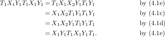 $$ \begin{align*} T_1X_1 Y_1T_1X_1 Y_1 &= T_1X_1 X_2Y_1T_1 Y_1 & & \text{by (4.1e)}\\ &= X_1X_2 T_1Y_1T_1 Y_1 & & \text{by (4.1c)} \\ &= X_1 X_2 Y_1 T_1Y_1T_1 & & \text{by (4.1d)} \\ &= X_1 Y_1T_1X_1 Y_1 T_1. & & \text{by (4.1e)} \end{align*} $$
The fact that $\mathfrak {a}$
is a morphism implies that
$\mathfrak {a}$
is a morphism implies that $\mathfrak {b}$
is a morphism since
$\mathfrak {b}$
is a morphism since
 $$ \begin{align*}\mathfrak{b}=\iota \mathfrak{a}\iota. \end{align*} $$
Remark that the quadratic relation (4.1b) was not used in the verification of the other relations. Therefore, $\mathfrak {a}$
,
$\mathfrak {a}$
, $\mathfrak {b}$
and
$\mathfrak {b}$
and $\iota $
are not only endomorphisms of
$\iota $
are not only endomorphisms of $\mathscr {H}^+$
but also endomorphisms of the underlying monoid.
$\mathscr {H}^+$
but also endomorphisms of the underlying monoid.
Proposition 4.6. The endomorphism $\mathfrak {a}$
and
$\mathfrak {a}$
and $\mathfrak {b}$
of
$\mathfrak {b}$
of $\mathscr {H}^+$
generate a free monoid.
$\mathscr {H}^+$
generate a free monoid.
Proof. The double affine Hecke algebra $\mathscr {H}_k$
has endomorphisms defined by the same formulas as
$\mathscr {H}_k$
has endomorphisms defined by the same formulas as $\mathfrak {a}$
,
$\mathfrak {a}$
, $\mathfrak {b}$
, with the obvious constraint on the label i. Indeed, with this definition,
$\mathfrak {b}$
, with the obvious constraint on the label i. Indeed, with this definition, $\mathfrak {a}$
and
$\mathfrak {a}$
and $\mathfrak {b}$
correspond, respectively, to
$\mathfrak {b}$
correspond, respectively, to $\rho _2$
and
$\rho _2$
and $\rho _1$
in [Reference Schiffmann and Vasserot25, §2.1] or to
$\rho _1$
in [Reference Schiffmann and Vasserot25, §2.1] or to $\mathfrak {a}$
and
$\mathfrak {a}$
and $\mathfrak {b}^{-1}$
in [Reference Ion and Sahi19, Chapter 6]. Furthermore, the corresponding
$\mathfrak {b}^{-1}$
in [Reference Ion and Sahi19, Chapter 6]. Furthermore, the corresponding $\mathfrak {a}$
,
$\mathfrak {a}$
, $\mathfrak {b}$
are in fact automorphisms of
$\mathfrak {b}$
are in fact automorphisms of $\mathscr {H}_k$
and generate a copy of the braid group on three strands (see, e.g., [Reference Ion and Sahi19, Theorem 6.4]). They stabilize the subalgebra
$\mathscr {H}_k$
and generate a copy of the braid group on three strands (see, e.g., [Reference Ion and Sahi19, Theorem 6.4]). They stabilize the subalgebra $\mathscr {H}^+_k$
, and the restrictions on
$\mathscr {H}^+_k$
, and the restrictions on $\mathfrak {a}$
,
$\mathfrak {a}$
, $\mathfrak {b}$
to
$\mathfrak {b}$
to $\mathscr {H}^+_k$
generate the free monoid on two generators. Since, as pointed out in Remark 4.4,
$\mathscr {H}^+_k$
generate the free monoid on two generators. Since, as pointed out in Remark 4.4, $\mathscr {H}^+_k$
is a quotient of the subalgebra
$\mathscr {H}^+_k$
is a quotient of the subalgebra $\mathscr {H}^+(k)\subseteq \mathscr {H}^+$
and
$\mathscr {H}^+(k)\subseteq \mathscr {H}^+$
and $\mathscr {H}^+(k)$
is stable under the action of
$\mathscr {H}^+(k)$
is stable under the action of $\mathfrak {a}$
and
$\mathfrak {a}$
and $\mathfrak {b}$
, we obtain that the endomorphisms
$\mathfrak {b}$
, we obtain that the endomorphisms $\mathfrak {a}$
,
$\mathfrak {a}$
, $\mathfrak {b}$
of
$\mathfrak {b}$
of $\mathscr {H}^+$
generate a free monoid.
$\mathscr {H}^+$
generate a free monoid.
Remark 4.7. We can regard the braid group on three strands $B_3$
as generated by
$B_3$
as generated by $\mathfrak {a}, \mathfrak {b}^{-1}$
satisfying the braid relation
$\mathfrak {a}, \mathfrak {b}^{-1}$
satisfying the braid relation
 $$ \begin{align*}\mathfrak{a}\mathfrak{b}^{-1}\mathfrak{a}=\mathfrak{b}^{-1}\mathfrak{a}\mathfrak{b}^{-1}. \end{align*} $$
There is a surjective group morphism $B_3\to \operatorname {\mathrm {SL}}(2,\mathbb Z)$
which maps
$B_3\to \operatorname {\mathrm {SL}}(2,\mathbb Z)$
which maps $\mathfrak {a}$
to
$\mathfrak {a}$
to $A= \begin {bmatrix}1&1\\ 0&1 \end {bmatrix}$
and
$A= \begin {bmatrix}1&1\\ 0&1 \end {bmatrix}$
and $\mathfrak {b}$
to
$\mathfrak {b}$
to $ B=\begin {bmatrix}1&0\\ 1&1 \end {bmatrix}$
. The image of the free monoid
$ B=\begin {bmatrix}1&0\\ 1&1 \end {bmatrix}$
. The image of the free monoid $B_3^+$
generated by
$B_3^+$
generated by $\mathfrak {a}$
and
$\mathfrak {a}$
and $\mathfrak {b}$
maps bijectively to the free monoid generated by A and B which consists of the set
$\mathfrak {b}$
maps bijectively to the free monoid generated by A and B which consists of the set $\operatorname {\mathrm {SL}}(2,\mathbb Z)^+$
of matrices with nonnegative integer entries.
$\operatorname {\mathrm {SL}}(2,\mathbb Z)^+$
of matrices with nonnegative integer entries.
Similar facts, pertaining to the algebra $\mathscr {H}^-$
, can be recorded with the help of the antimorphism
$\mathscr {H}^-$
, can be recorded with the help of the antimorphism $\mathfrak {e}$
.
$\mathfrak {e}$
.
4.4
It is important to remark that the algebras $\mathscr {H}_k^+$
,
$\mathscr {H}_k^+$
, $k\geq 2$
, do not form an inverse system in any natural way and therefore
$k\geq 2$
, do not form an inverse system in any natural way and therefore $\mathscr {H}^+$
cannot be directly thought of as an inverse limit of
$\mathscr {H}^+$
cannot be directly thought of as an inverse limit of $\mathscr {H}_k^+$
,
$\mathscr {H}_k^+$
, $k\geq 2$
. However, we will show that both
$k\geq 2$
. However, we will show that both $\mathscr {H}^{\pm }$
acquire natural representations that are constructed by considering inverse systems built from the standard representations of
$\mathscr {H}^{\pm }$
acquire natural representations that are constructed by considering inverse systems built from the standard representations of $\mathscr {H}_k^{\pm }$
,
$\mathscr {H}_k^{\pm }$
, $k\geq 2$
.
$k\geq 2$
.
5 The standard representation of the ${}^{-}$
stable limit DAHA
${}^{-}$
stable limit DAHA

5.1
The results in the remainder of this section are due to Knop [Reference Knop21]. We briefly recall here the emerging structure. We refer to §2.5 for the relevant notation. The map $\pi _k:\mathscr {P}^-_k\rightarrow \mathscr {P}^-_{k-1}$
is partially compatible with the actions of
$\pi _k:\mathscr {P}^-_k\rightarrow \mathscr {P}^-_{k-1}$
is partially compatible with the actions of $\mathscr {A}_k^-$
and
$\mathscr {A}_k^-$
and $\mathscr {A}_{k-1}^-$
. More precisely,
$\mathscr {A}_{k-1}^-$
. More precisely,
 $$ \begin{align} \begin{split} \pi_k T_i &= T_i \pi_k,\quad 1\leq i\leq k-2,\\ \pi_k \widetilde{\omega}_k &= 0, \\ \pi_k T_{k-1}\widetilde{\omega}_k & = \widetilde{\omega}_{k-1}\pi_k,\\ \pi_k X_i^{-1} &= X_{i}^{-1}\pi_k,\quad 1\leq i\leq k-1,\\ \pi_k X_k^{-1} &= 0. \end{split} \end{align} $$
We refer to [Reference Knop21, Theorem 9.1] for the details.
5.2
The compatibility with the actions of $\mathscr {H}_k^{-}$
and
$\mathscr {H}_k^{-}$
and $\mathscr {H}_{k-1}^{-}$
can also be investigated, but the verification is more delicate. More precisely, we have the following result [Reference Knop21, Proposition 9.11].
$\mathscr {H}_{k-1}^{-}$
can also be investigated, but the verification is more delicate. More precisely, we have the following result [Reference Knop21, Proposition 9.11].
Proposition 5.1. For any $1\leq i\leq k-1$
, we have
$1\leq i\leq k-1$
, we have
 $$ \begin{align} \pi_k Y_i= Y_{i}\pi_k. \end{align} $$
Furthermore, the operator $Y^{-1}_i$
stabilizes both
$Y^{-1}_i$
stabilizes both $\mathscr {P}_k^{-}$
and
$\mathscr {P}_k^{-}$
and $\mathscr {P}_{k-1}^-$
and
$\mathscr {P}_{k-1}^-$
and
 $$ \begin{align} \pi_k Y^{-1}_i= Y^{-1}_{i}\pi_k. \end{align} $$
5.3
For any $n\geq 1$
, the sequence of operators
$n\geq 1$
, the sequence of operators $(A_k)_{k\geq 1}$
defined by
$(A_k)_{k\geq 1}$
defined by
 $$ \begin{align*} A_k:=Y_n^{(k)}, \quad k\geq n, \end{align*} $$
induces the limit operator $\displaystyle \mathscr {Y}_n:\lim _{\substack {\longleftarrow \\ k\geq n}} \mathscr {P}_k^-\to \lim _{\substack {\longleftarrow \\ k\geq n}} \mathscr {P}_k^-$
. Since
$\displaystyle \mathscr {Y}_n:\lim _{\substack {\longleftarrow \\ k\geq n}} \mathscr {P}_k^-\to \lim _{\substack {\longleftarrow \\ k\geq n}} \mathscr {P}_k^-$
. Since $\displaystyle \lim _{\substack {\longleftarrow \\ k\geq n}} \mathscr {P}_k$
and
$\displaystyle \lim _{\substack {\longleftarrow \\ k\geq n}} \mathscr {P}_k$
and $\mathscr {P}^-_{\infty }$
are canonically isomorphic, we obtain an operator
$\mathscr {P}^-_{\infty }$
are canonically isomorphic, we obtain an operator $\displaystyle \mathscr {Y}_n:\mathscr {P}^-\to \mathscr {P}^-$
. Similarly, we obtain the limit operators
$\displaystyle \mathscr {Y}_n:\mathscr {P}^-\to \mathscr {P}^-$
. Similarly, we obtain the limit operators $\mathscr {T}_i, \mathscr {X}^{-1}_i$
, and
$\mathscr {T}_i, \mathscr {X}^{-1}_i$
, and $\mathscr {Y}^{-1}_i$
,
$\mathscr {Y}^{-1}_i$
, $i\geq 1$
. It is important to remark that the operators
$i\geq 1$
. It is important to remark that the operators $\mathscr {Y}^{-1}_i$
are invertible (with inverse
$\mathscr {Y}^{-1}_i$
are invertible (with inverse $\mathscr {Y}_i$
). The following result immediately follows.
$\mathscr {Y}_i$
). The following result immediately follows.
Theorem 5.2. The limit operators $\mathscr {T}_i, \mathscr {X}^{-1}_i$
, and
$\mathscr {T}_i, \mathscr {X}^{-1}_i$
, and $\mathscr {Y}^{-1}_i$
,
$\mathscr {Y}^{-1}_i$
, $i\geq 1$
, define an
$i\geq 1$
, define an $\mathscr {H}^{-}$
action on
$\mathscr {H}^{-}$
action on $\mathscr {P}^-_{\infty }$
.
$\mathscr {P}^-_{\infty }$
.
Proof. All relations are satisfied because they are satisfied by the corresponding operators acting on each $\mathscr {P}_k^{-}$
.
$\mathscr {P}_k^{-}$
.
5.4
As it was pointed out in [Reference Knop21, §10] the almost symmetric module $\mathscr {P}_{\mathrm {as}}^-$
, defined in §2.7, is a
$\mathscr {P}_{\mathrm {as}}^-$
, defined in §2.7, is a $\mathscr {H}^-$
-stable subspace of
$\mathscr {H}^-$
-stable subspace of $\mathscr {P}_{\infty }^-$
and is more canonical from a certain point of view. Specifically, each
$\mathscr {P}_{\infty }^-$
and is more canonical from a certain point of view. Specifically, each $\mathscr {P}_k^-$
is a parabolic module for the affine Hecke algebra
$\mathscr {P}_k^-$
is a parabolic module for the affine Hecke algebra $\mathscr {A}_k^-$
and has a standard basis (in the sense of Kazhdan-Lusztig theory) indexed by compositions with at most k parts. The sequences consisting of the standard basis elements indexed by the same composition (in all
$\mathscr {A}_k^-$
and has a standard basis (in the sense of Kazhdan-Lusztig theory) indexed by compositions with at most k parts. The sequences consisting of the standard basis elements indexed by the same composition (in all $\mathscr {P}_k^-$
,
$\mathscr {P}_k^-$
, $k\geq n$
, for some n) give elements of
$k\geq n$
, for some n) give elements of $\mathscr {P}_{\infty }^-$
(see [Reference Knop21, §9]) which are expected to play the role of a standard basis for the limit representation. However, these limits of standard basis elements do not span
$\mathscr {P}_{\infty }^-$
(see [Reference Knop21, §9]) which are expected to play the role of a standard basis for the limit representation. However, these limits of standard basis elements do not span $\mathscr {P}_{\infty }^-$
but rather the smaller space
$\mathscr {P}_{\infty }^-$
but rather the smaller space $\mathscr {P}_{\mathrm {as}}^-$
.
$\mathscr {P}_{\mathrm {as}}^-$
.
Theorem 5.3. The almost symmetric module $\mathscr {P}_{\mathrm {as}}^-$
is a
$\mathscr {P}_{\mathrm {as}}^-$
is a $\mathscr {H}^{-}$
-submodule of
$\mathscr {H}^{-}$
-submodule of $\mathscr {P}^-_{\infty }$
.
$\mathscr {P}^-_{\infty }$
.
We call this representation the standard representation of $\mathscr {H}^-$
. We expect this representation to be faithful.
$\mathscr {H}^-$
. We expect this representation to be faithful.
As explained in [Reference Knop21], a sequence on nonsymmetric Macdonald polynomials indexed by the same composition gives rise to an element of $\mathscr {P}_{\mathrm {as}}^-$
, and such elements are common eigenfunctions for the action the operators
$\mathscr {P}_{\mathrm {as}}^-$
, and such elements are common eigenfunctions for the action the operators $\mathscr {Y}^{-1}_i$
. The limit nonsymmetric Macdonald polynomials do not span
$\mathscr {Y}^{-1}_i$
. The limit nonsymmetric Macdonald polynomials do not span $\mathscr {P}_{\mathrm {as}}^-$
, and therefore the spectral theory of the operators
$\mathscr {P}_{\mathrm {as}}^-$
, and therefore the spectral theory of the operators $\mathscr {Y}^{-1}_i$
acting on
$\mathscr {Y}^{-1}_i$
acting on $\mathscr {P}_{\mathrm {as}}^-$
is not yet fully understood.
$\mathscr {P}_{\mathrm {as}}^-$
is not yet fully understood.
6 The standard representation of the
${}^{+}$
stable limit DAHA

6.1
Before delving into this section, which is the technical core of the article, it might be helpful to offer a summary of the difficulties that one encounters in the effort to understand the limiting behaviour of the Cherednik operators (the analysis of all the other generators of $\mathscr {H}_k^+$
is straightforward) in relationship to the inverse system
$\mathscr {H}_k^+$
is straightforward) in relationship to the inverse system $(\mathscr {P}_k^+)_{k\geq 2}$
, as well as provide a less technical description of the new elements that are employed to describe this limiting behaviour.
$(\mathscr {P}_k^+)_{k\geq 2}$
, as well as provide a less technical description of the new elements that are employed to describe this limiting behaviour.
It has been known to the specialists that the Cherednik operators $Y^{(k)}_i$
are not compatible with the inverse system
$Y^{(k)}_i$
are not compatible with the inverse system $(\mathscr {P}_k^+)_{k\geq 2}$
. Our first observation is that the family of operators
$(\mathscr {P}_k^+)_{k\geq 2}$
. Our first observation is that the family of operators $\textbf {t}^kY^{(k)}_i$
, for fixed i, are compatible with inverse system
$\textbf {t}^kY^{(k)}_i$
, for fixed i, are compatible with inverse system $(x_i\mathscr {P}_k^+)_{k\geq 2}$
, which does lead to a limit operator acting on
$(x_i\mathscr {P}_k^+)_{k\geq 2}$
, which does lead to a limit operator acting on $x_i\mathscr {P}_{\infty }^+$
. However, there is no common domain for all limit operators
$x_i\mathscr {P}_{\infty }^+$
. However, there is no common domain for all limit operators $Y_i$
,
$Y_i$
, $i\geq 1$
. To address this situation, we consider some modified operators acting on
$i\geq 1$
. To address this situation, we consider some modified operators acting on $\mathscr {P}_k^+$
, which we denote by
$\mathscr {P}_k^+$
, which we denote by $\widetilde {Y}_i^{(k)}$
. Like the Cherednik operators, these operators satisfy the relations
$\widetilde {Y}_i^{(k)}$
. Like the Cherednik operators, these operators satisfy the relations $\widetilde {Y}^{(k)}_{i+1}=\textbf {t}^{-1} T_i \widetilde {Y}^{(k)}_i T_i$
,
$\widetilde {Y}^{(k)}_{i+1}=\textbf {t}^{-1} T_i \widetilde {Y}^{(k)}_i T_i$
, $1\leq i\leq k-1$
,
$1\leq i\leq k-1$
, $T_j \widetilde {Y}^{(k)}_i=\widetilde {Y}^{(k)}_i T_j$
,
$T_j \widetilde {Y}^{(k)}_i=\widetilde {Y}^{(k)}_i T_j$
, $|i-j|>1$
, and are therefore fully determined by the operator
$|i-j|>1$
, and are therefore fully determined by the operator $\widetilde {Y}^{(k)}_{1}$
, which has the following additional properties
$\widetilde {Y}^{(k)}_{1}$
, which has the following additional properties
-
i)
$\widetilde {Y}_1^{(k)}=\textbf {t}^k Y_1^{(k)}$
on
$x_1\mathscr {P}_k^+$
; -
ii)
$\widetilde {Y}_1^{(k)}\cdot \mathscr {P}_k^+\subseteq x_1\mathscr {P}_k^+$
.


The first property implies that $\widetilde {Y}_i^{(k)}=\textbf {t}^k Y_i^{(k)}$
on
$\widetilde {Y}_i^{(k)}=\textbf {t}^k Y_i^{(k)}$
on $x_i\mathscr {P}_k^+$
for all
$x_i\mathscr {P}_k^+$
for all $1\leq i \leq k$
; the second property implies that
$1\leq i \leq k$
; the second property implies that $\widetilde {Y}_i^{(k)}\cdot \mathscr {P}_k^+\subseteq T_{i-1}\cdots T_1 x_1\mathscr {P}_k^+$
for all
$\widetilde {Y}_i^{(k)}\cdot \mathscr {P}_k^+\subseteq T_{i-1}\cdots T_1 x_1\mathscr {P}_k^+$
for all $1\leq i \leq k$
. The operator for
$1\leq i \leq k$
. The operator for $\widetilde {Y}_1^{(k)}$
is obtained by projecting the action of
$\widetilde {Y}_1^{(k)}$
is obtained by projecting the action of $Y_1^{(k)}$
onto the space
$Y_1^{(k)}$
onto the space $x_1\mathscr {P}_k^+$
.
$x_1\mathscr {P}_k^+$
.
The structural properties of the algebra generated by $\widetilde {Y}_i^{(k)}$
,
$\widetilde {Y}_i^{(k)}$
, $X_i$
,
$X_i$
, $1\leq k$
, and
$1\leq k$
, and $T_i$
,
$T_i$
, $1\leq i\leq k-1$
are used to define an algebraic structure
$1\leq i\leq k-1$
are used to define an algebraic structure $\widetilde {\mathscr {H}}_k^+$
called the deformed DAHA.
$\widetilde {\mathscr {H}}_k^+$
called the deformed DAHA. $\widetilde {\mathscr {H}}_k^+$
has a natural action
$\widetilde {\mathscr {H}}_k^+$
has a natural action $\mathscr {P}_k^+$
(the standard representation), which is related to the standard representation of
$\mathscr {P}_k^+$
(the standard representation), which is related to the standard representation of $\mathscr {H}_k^+$
on
$\mathscr {H}_k^+$
on $\mathscr {P}_k^+$
in the manner described above.
$\mathscr {P}_k^+$
in the manner described above.
The modified Cherednik operators $\widetilde {Y}_i^{(k)}$
, for fixed i, are not yet compatible with the inverse system
$\widetilde {Y}_i^{(k)}$
, for fixed i, are not yet compatible with the inverse system $(\mathscr {P}_k^+)_{k\geq 2}$
, but they are quite close to satisfying such a property. To be able to point out more precisely what happens, we first remark that they act consistently on constant sequences (i.e., sequences compatible with the canonical inclusions
$(\mathscr {P}_k^+)_{k\geq 2}$
, but they are quite close to satisfying such a property. To be able to point out more precisely what happens, we first remark that they act consistently on constant sequences (i.e., sequences compatible with the canonical inclusions $\iota _k: \mathscr {P}_{k-1}^+\to \mathscr {P}_k^+$
) in this inverse system (Lemma 6.10). This fact implies the existence of limit operators defined on
$\iota _k: \mathscr {P}_{k-1}^+\to \mathscr {P}_k^+$
) in this inverse system (Lemma 6.10). This fact implies the existence of limit operators defined on
 $$ \begin{align*} \displaystyle{\lim_{{\longrightarrow}}} \mathscr{P}_k^+=\mathbb Q(\textbf{t},\textbf{q})[x_1,x_2,\dots], \end{align*} $$
the ring of polynomials in infinitely many variables, but still not on $\mathscr {P}_{\infty }^+$
. Interestingly, the image of
$\mathscr {P}_{\infty }^+$
. Interestingly, the image of $\displaystyle {\lim _{{\longrightarrow }}} \mathscr {P}_k^+$
under the limit operators lies in
$\displaystyle {\lim _{{\longrightarrow }}} \mathscr {P}_k^+$
under the limit operators lies in $\mathscr {P}_{\mathrm {as}}^+$
(which is strictly smaller than
$\mathscr {P}_{\mathrm {as}}^+$
(which is strictly smaller than $\mathscr {P}_{\infty }^+$
), showing that the smallest space on which one can hope to acquire an action of an algebra of limit operators is
$\mathscr {P}_{\infty }^+$
), showing that the smallest space on which one can hope to acquire an action of an algebra of limit operators is $\mathscr {P}_{\mathrm {as}}^+$
.
$\mathscr {P}_{\mathrm {as}}^+$
.
In order to understand the failure of the diagram
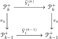
to be commutative, we can consider the difference $\pi _k \widetilde {Y}_{1}^{(k)} - \widetilde {Y}_{1}^{(k-1)} \pi _k: \mathscr {P}_k^+\to \mathscr {P}_{k-1}^+$
. On the subspace
$\pi _k \widetilde {Y}_{1}^{(k)} - \widetilde {Y}_{1}^{(k-1)} \pi _k: \mathscr {P}_k^+\to \mathscr {P}_{k-1}^+$
. On the subspace $x_k\mathscr {P}_k^+$
, this difference has no kernel and reduces to
$x_k\mathscr {P}_k^+$
, this difference has no kernel and reduces to $\pi _k \widetilde {Y}_{1}^{(k)} : x_k\mathscr {P}_k^+\to \mathscr {P}_{k-1}^+$
. Since for every monomial in
$\pi _k \widetilde {Y}_{1}^{(k)} : x_k\mathscr {P}_k^+\to \mathscr {P}_{k-1}^+$
. Since for every monomial in $m\in \mathbb Q(\textbf {t},\textbf {q})[x_1,x_2,\dots ]$
there exists a unique k such that
$m\in \mathbb Q(\textbf {t},\textbf {q})[x_1,x_2,\dots ]$
there exists a unique k such that $m\in x_k\mathscr {P}_k^+$
, we can use the action of
$m\in x_k\mathscr {P}_k^+$
, we can use the action of $\pi _k \widetilde {Y}_{1}^{(k)}$
on
$\pi _k \widetilde {Y}_{1}^{(k)}$
on $x_k\mathscr {P}_k^+$
to define an operator
$x_k\mathscr {P}_k^+$
to define an operator
 $$ \begin{align*} W_1: \mathbb Q(\textbf{t},\textbf{q})[x_1,x_2,\dots]\to \mathbb Q(\textbf{t},\textbf{q})[x_1,x_2,\dots] \end{align*} $$
such that $W_1=\pi _k \widetilde {Y}_{1}^{(k)}$
on
$W_1=\pi _k \widetilde {Y}_{1}^{(k)}$
on $x_k\mathscr {P}_k^+$
. By restricting
$x_k\mathscr {P}_k^+$
. By restricting $W_1$
to
$W_1$
to $\mathscr {P}_k^+$
, we obtain the operator
$\mathscr {P}_k^+$
, we obtain the operator $W_1^{(k)}: \mathscr {P}_k^+\to \mathscr {P}_k^+$
. We can regard the operator
$W_1^{(k)}: \mathscr {P}_k^+\to \mathscr {P}_k^+$
. We can regard the operator $W_1$
as collecting some obvious obstructions to the commutativity of the above diagram.
$W_1$
as collecting some obvious obstructions to the commutativity of the above diagram.
As it turns out, these are all the obstructions to the commutativity of the diagram: If $ \widetilde {Z}_{1}^{(k)}= \widetilde {Y}_{1}^{(k)} - W_1^{(k)}$
, then the corresponding diagram for the
$ \widetilde {Z}_{1}^{(k)}= \widetilde {Y}_{1}^{(k)} - W_1^{(k)}$
, then the corresponding diagram for the $ \widetilde {Z}_{1}^{(k)} $
operators is commutative, leading to an operator
$ \widetilde {Z}_{1}^{(k)} $
operators is commutative, leading to an operator
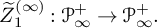 $$ \begin{align*} \widetilde{Z}_{1}^{(\infty)}: \mathscr{P}_{\infty}^+\to \mathscr{P}_{\infty}^+. \end{align*} $$
Furthermore, the action of $W_1$
(or
$W_1$
(or $W_1^{(k)}$
) on monomials can be explicitly computed; this is the action described in §6.8. Since this action is particularly simple, we were able to compute the action of the operators
$W_1^{(k)}$
) on monomials can be explicitly computed; this is the action described in §6.8. Since this action is particularly simple, we were able to compute the action of the operators $W_1^{(k)}$
on sequences in the inverse system
$W_1^{(k)}$
on sequences in the inverse system $(\mathscr {P}_k^+)_{k\geq 2}$
. This computation revealed that if the sequence in the inverse system has limit in
$(\mathscr {P}_k^+)_{k\geq 2}$
. This computation revealed that if the sequence in the inverse system has limit in $\mathscr {P}_{\mathrm {as}}^+$
, then one obtains by applying
$\mathscr {P}_{\mathrm {as}}^+$
, then one obtains by applying $W_1^{(k)}$
another sequence in
$W_1^{(k)}$
another sequence in $(\mathscr {P}_k^+)_{k\geq 2}$
which can be written as a finite linear expression of sequences compatible with the inverse system. The coefficients in these linear expressions are sequences in
$(\mathscr {P}_k^+)_{k\geq 2}$
which can be written as a finite linear expression of sequences compatible with the inverse system. The coefficients in these linear expressions are sequences in $\mathbb Q(\textbf {t},\textbf {q})$
that are convergent in the
$\mathbb Q(\textbf {t},\textbf {q})$
that are convergent in the $\textbf {t}$
-adic topology (i.e.,
$\textbf {t}$
-adic topology (i.e., $\textbf {t}$
is treated as a small positive real number). This led us to the concept of limit described in §6.9. We refer to the sequences that have limit in this sense as convergent sequences.
$\textbf {t}$
is treated as a small positive real number). This led us to the concept of limit described in §6.9. We refer to the sequences that have limit in this sense as convergent sequences.
Since both ${W}_i^{(k)}$
and
${W}_i^{(k)}$
and $\widetilde {Z}_i^{(k)}$
have limit in this sense, we obtain that the operators
$\widetilde {Z}_i^{(k)}$
have limit in this sense, we obtain that the operators $\widetilde {Y}_i^{(k)}$
have limit (denoted by
$\widetilde {Y}_i^{(k)}$
have limit (denoted by $\mathscr {Y}_i$
). Although, the co-domain for the limit operators
$\mathscr {Y}_i$
). Although, the co-domain for the limit operators ${W}_i^{(\infty )}$
and
${W}_i^{(\infty )}$
and $\widetilde {Z}_i^{(\infty )}$
is, in general,
$\widetilde {Z}_i^{(\infty )}$
is, in general, $\mathscr {P}_{\infty }^+$
, it turns out that
$\mathscr {P}_{\infty }^+$
, it turns out that $\mathscr {Y}_i: \mathscr {P}_{\mathrm {as}}^+\to \mathscr {P}_{\mathrm {as}}^+$
. Furthermore,
$\mathscr {Y}_i: \mathscr {P}_{\mathrm {as}}^+\to \mathscr {P}_{\mathrm {as}}^+$
. Furthermore, $\mathscr {Y}_i$
satisfies a continuity property: It sends convergent sequences to convergent sequences.
$\mathscr {Y}_i$
satisfies a continuity property: It sends convergent sequences to convergent sequences.
The analysis of the algebraic structure generated by the action of the limit operators $\mathscr {Y}_i$
makes use of the continuity property. Their most remarkable property of the limit operators is their commutativity. The commutativity holds, of course, for the finite rank Cherednik operators, but it does not hold for the modified Cherednik operators, and it was interesting to discover that the commutativity is restored in the limit. Furthermore, the action of
$\mathscr {Y}_i$
makes use of the continuity property. Their most remarkable property of the limit operators is their commutativity. The commutativity holds, of course, for the finite rank Cherednik operators, but it does not hold for the modified Cherednik operators, and it was interesting to discover that the commutativity is restored in the limit. Furthermore, the action of $\mathscr {Y}_i$
on
$\mathscr {Y}_i$
on $x_i\mathscr {P}_{\mathrm {as}}^+$
matches the action of the corresponding limit Cherednik operator
$x_i\mathscr {P}_{\mathrm {as}}^+$
matches the action of the corresponding limit Cherednik operator $Y_i$
. Ultimately, the action of the limit operators
$Y_i$
. Ultimately, the action of the limit operators $\mathscr {Y}_i$
,
$\mathscr {Y}_i$
, $\mathscr {X}_i$
, and
$\mathscr {X}_i$
, and $\mathscr {T}_i$
define an action of
$\mathscr {T}_i$
define an action of $\mathscr {H}^+$
on
$\mathscr {H}^+$
on $\mathscr {P}_{\mathrm {as}}^+$
.
$\mathscr {P}_{\mathrm {as}}^+$
.
6.2
The map $\pi _k:\mathscr {P}^+_k\rightarrow \mathscr {P}^+_{k-1}$
is also partially compatible with the actions of
$\pi _k:\mathscr {P}^+_k\rightarrow \mathscr {P}^+_{k-1}$
is also partially compatible with the actions of $\mathscr {A}_k^+$
and
$\mathscr {A}_k^+$
and $\mathscr {A}_{k-1}^+$
. More precisely,
$\mathscr {A}_{k-1}^+$
. More precisely,
 $$ \begin{align} \pi_k T_i &= T_i \pi_k,\quad 1\leq i\leq k-2,\nonumber\\ \pi_k T_{k-1}^{-1}\dots T_1^{-1}\widetilde{\omega}_k^{-1} &= 0\nonumber \\ \pi_k \widetilde{\omega}_k^{-1}T_{k-1} & = \widetilde{\omega}_{k-1}^{-1}\pi_k\\ \pi_k X_i &= X_{i}\pi_k,\quad 1\leq i\leq k-1,\nonumber \\ \pi_k X_i &= 0.\nonumber\end{align} $$
As before, these relations show that the operators $T_i$
and
$T_i$
and $X_i$
have limits (in the sense of §5.3), denoted by
$X_i$
have limits (in the sense of §5.3), denoted by $\mathscr {T}_i$
and
$\mathscr {T}_i$
and $\mathscr {X}_i$
, that act on
$\mathscr {X}_i$
, that act on $\mathscr {P}_{\infty }^+$
.
$\mathscr {P}_{\infty }^+$
.
6.3
On the other hand, for any $i\geq 1$
, the actions of the operators
$i\geq 1$
, the actions of the operators $Y^{(k)}_{i}$
and
$Y^{(k)}_{i}$
and $Y^{(k-1)}_{i}$
are no longer compatible with the map
$Y^{(k-1)}_{i}$
are no longer compatible with the map $\pi _k$
. One immediate obstruction is the fact that the eigenvalues of
$\pi _k$
. One immediate obstruction is the fact that the eigenvalues of $Y_{i}$
on
$Y_{i}$
on $\mathscr {P}_k^+$
and
$\mathscr {P}_k^+$
and $\mathscr {P}_{k-1}^+$
no longer match, as is was the case for their action on
$\mathscr {P}_{k-1}^+$
no longer match, as is was the case for their action on $\mathscr {P}_k^-$
and
$\mathscr {P}_k^-$
and $\mathscr {P}_{k-1}^-$
. The common spectrum of the action of
$\mathscr {P}_{k-1}^-$
. The common spectrum of the action of $Y_i$
,
$Y_i$
, $1\leq i\leq k$
, on
$1\leq i\leq k$
, on $\mathscr {P}_k^+$
is known from type
$\mathscr {P}_k^+$
is known from type $A_{k-1}$
Macdonald theory. The common eigenfunctions are nonsymmetric Macdonald polynomials; they are indexed by compositions
$A_{k-1}$
Macdonald theory. The common eigenfunctions are nonsymmetric Macdonald polynomials; they are indexed by compositions $\lambda =(\lambda _1,\dots ,\lambda _k)\in \mathbb Z_{\geq 0}^k$
. The eigenvalue of
$\lambda =(\lambda _1,\dots ,\lambda _k)\in \mathbb Z_{\geq 0}^k$
. The eigenvalue of $Y^{(k)}_i$
corresponding to the nonsymmetric Macdonald polynomial indexed by
$Y^{(k)}_i$
corresponding to the nonsymmetric Macdonald polynomial indexed by $\lambda $
is
$\lambda $
is
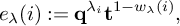 $$ \begin{align*} e_{\lambda}(i):=\textbf{q}^{\lambda_i}\textbf{t}^{1-w_{\lambda}(i)}, \end{align*} $$
where $w_{\lambda }(i)=|\{j=1,\dots ,i~|~\lambda _j\leq \lambda _i\}|+|\{j=1,\dots ,i~|~\lambda _j< \lambda _i\}|$
. For the composition
$w_{\lambda }(i)=|\{j=1,\dots ,i~|~\lambda _j\leq \lambda _i\}|+|\{j=1,\dots ,i~|~\lambda _j< \lambda _i\}|$
. For the composition $(\lambda ,0)\in \mathbb Z_{\geq 0}^{k+1}$
, we have
$(\lambda ,0)\in \mathbb Z_{\geq 0}^{k+1}$
, we have
 $$ \begin{align*} e_{(\lambda,0)}(i)=e_{\lambda}(i)\textbf{t}^{-1},\quad \text{if } \lambda_i>0, \quad \text{and}\quad e_{(\lambda,0)}(i)=e_{\lambda}(i),\quad \text{if } \lambda_i=0. \end{align*} $$
One way to partially correct this problem is to consider the normalized operators $\textbf {t}^{k}Y^{(k)}_i$
. Comparing the eigenvalues corresponding to
$\textbf {t}^{k}Y^{(k)}_i$
. Comparing the eigenvalues corresponding to $\lambda $
and
$\lambda $
and $(\lambda ,0)$
gives
$(\lambda ,0)$
gives
 $$ \begin{align*} \textbf{t}^{k+1}e_{(\lambda,0)}(i)=\textbf{t}^k e_{\lambda}(i),\quad \text{if } \lambda_i>0, \quad \text{and}\quad \textbf{t}^{k+1} e_{(\lambda,0)}(i)=\textbf{t}^k e_{\lambda}(i)\cdot \textbf{t},\quad \text{if } \lambda_i=0. \end{align*} $$
Example 6.1. The discrepancy between the eigenvalues is also reflected in the eigenfunctions. For example, the Macdonald polynomial corresponding to the compositions $(0,1,0)$
and
$(0,1,0)$
and $(0,1)$
are, respectively,
$(0,1)$
are, respectively,
 $$ \begin{align*} x_2+\frac{\textbf{q}(1-\textbf{t})}{\textbf{q}-\textbf{t}^2}x_1\quad\quad \text{and}\quad\quad x_2+\frac{\textbf{q}(1-\textbf{t})}{\textbf{q}-\textbf{t}}x_1. \end{align*} $$
This shows, in particular, that $\pi _3 Y_1^{(3)}\neq Y_1^{(2)}\pi _3$
.
$\pi _3 Y_1^{(3)}\neq Y_1^{(2)}\pi _3$
.
6.4
A crucial observation is that the actions of the operators $\textbf {t}^{k}Y^{(k)}_iX^{(k)}_i\in \mathscr {H}_k^{+}$
on
$\textbf {t}^{k}Y^{(k)}_iX^{(k)}_i\in \mathscr {H}_k^{+}$
on $\mathscr {P}_{k}^{+}$
are compatible with the inverse system.
$\mathscr {P}_{k}^{+}$
are compatible with the inverse system.
Proposition 6.2. For any $1\leq i\leq k-1$
, we have
$1\leq i\leq k-1$
, we have
 $$ \begin{align*} \pi_k\textbf{t}^{k}Y_i X_i=\textbf{t}^{k-1}Y_iX_i\pi_k. \end{align*} $$
Proof. First note that we have
 $$ \begin{align} \pi_k\omega^{-1}_k T_{k-1}= \omega^{-1}_{k-1}\pi_k, \end{align} $$
which can be verified by direct computation. Hence, by equation 6.1 we have
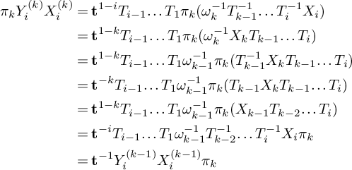 $$ \begin{align*} \pi_k Y_i^{(k)}X_i^{(k)}&= \textbf{t}^{1-i}T_{i-1} \dots T_{1}\pi_k(\omega^{-1}_k T_{k-1}^{-1}\dots T_{i}^{-1}X_i)\\ &=\textbf{t}^{1-k}T_{i-1} \dots T_{1}\pi_k(\omega^{-1}_k X_kT_{k-1}\dots T_{i})\\ &=\textbf{t}^{1-k}T_{i-1} \dots T_{1}\omega^{-1}_{k-1}\pi_k( T_{k-1}^{-1}X_kT_{k-1}\dots T_{i})\\ &=\textbf{t}^{-k}T_{i-1} \dots T_{1}\omega^{-1}_{k-1}\pi_k( T_{k-1}X_kT_{k-1}\dots T_{i})\\ &=\textbf{t}^{1-k}T_{i-1} \dots T_{1}\omega^{-1}_{k-1}\pi_k( X_{k-1}T_{k-2}\dots T_{i})\\ &=\textbf{t}^{-i}T_{i-1} \dots T_{1}\omega^{-1}_{k-1}T_{k-2}^{-1}\dots T_{i}^{-1}X_i\pi_k\\ &=\textbf{t}^{-1}Y_i^{(k-1)}X_i^{(k-1)}\pi_k \end{align*} $$
Therefore, we have $\pi _k\textbf {t}^{k}Y_i^{(k)}X^{(k)}_i=\textbf {t}^{k-1}Y_i^{(k-1)}X^{(k-1)}_i\pi _k$
.
$\pi _k\textbf {t}^{k}Y_i^{(k)}X^{(k)}_i=\textbf {t}^{k-1}Y_i^{(k-1)}X^{(k-1)}_i\pi _k$
.
In other words, one can obtain a limit operator corresponding to $Y_i$
, acting on the space
$Y_i$
, acting on the space $x_i\mathscr {P}_{\infty }^+\subset \mathscr {P}_{\infty }^+$
. However, this is not satisfactory because it does not produce a nontrivial common domain for all the limit operators
$x_i\mathscr {P}_{\infty }^+\subset \mathscr {P}_{\infty }^+$
. However, this is not satisfactory because it does not produce a nontrivial common domain for all the limit operators $Y_i$
,
$Y_i$
, $i\geq 1$
. In order to extend the action of the limit operator
$i\geq 1$
. In order to extend the action of the limit operator $Y_i$
to a larger domain, we introduce the deformed double affine Hecke algebras and the concept of limit detailed in §6.9.
$Y_i$
to a larger domain, we introduce the deformed double affine Hecke algebras and the concept of limit detailed in §6.9.
6.5 The deformed double affine Hecke algebras
Definition 6.3. The deformed DAHA $\widetilde {\mathscr {H}}_{k}^{+}$
,
$\widetilde {\mathscr {H}}_{k}^{+}$
, $k\geq 2$
, is the
$k\geq 2$
, is the $\mathbb {Q}(\textbf {t},\textbf {q})$
-algebra generated by the elements
$\mathbb {Q}(\textbf {t},\textbf {q})$
-algebra generated by the elements $T_1,\dots ,T_{k-1}$
,
$T_1,\dots ,T_{k-1}$
, $X_1,\dots ,X_k$
and
$X_1,\dots ,X_k$
and $\varpi _k$
satisfying equations (3.1a), (3.1b) and (3.1c) and the following relations:
$\varpi _k$
satisfying equations (3.1a), (3.1b) and (3.1c) and the following relations:
 $$ \begin{align} \begin{gathered} \varpi_kT_i=T_{i+1}\varpi_k, \quad 1\leq i\leq k-2,\\ \varpi_kX_i=X_{i+1}\varpi_k,\quad 1\leq i\leq k-1, \end{gathered} \end{align} $$
 $$ \begin{align} \begin{gathered} \gamma_k T_{k-1}=-\textbf{t} \gamma_k,\quad T_1\gamma_k =\gamma_k,\\ \gamma_k\varpi_k^{k-2}\gamma_k=\gamma_k\varpi_k^{k-1}\gamma_k=\gamma_k\varpi_k^{k}=0, \end{gathered} \end{align} $$
where
 $$ \begin{align*} \gamma_k=\varpi_k^2 T_{k-1}-T_{1}\varpi_k^2. \end{align*} $$
Remark 6.4. The quotient of $\widetilde {\mathscr {H}}_k^+$
by the ideal generated by
$\widetilde {\mathscr {H}}_k^+$
by the ideal generated by $\gamma _k$
is isomorphic to
$\gamma _k$
is isomorphic to $\mathscr {H}_k^+$
. As it is clear from the relations (6.4),
$\mathscr {H}_k^+$
. As it is clear from the relations (6.4), $\gamma _k$
is not central in
$\gamma _k$
is not central in $\widetilde {\mathscr {H}}_k^+$
.
$\widetilde {\mathscr {H}}_k^+$
.
Notation 6.5. Let $\widetilde {Y}_i$
,
$\widetilde {Y}_i$
, $1\leq i\leq k$
, be defined as follows
$1\leq i\leq k$
, be defined as follows
 $$ \begin{align*} \widetilde{Y}_1=\textbf{t}^{k}\varpi_kT_{k-1}^{-1}\dots T_1^{-1},\qquad \widetilde{Y}_{i+1}=\textbf{t}^{-1} T_i \widetilde{Y}_i T_i, \quad 1\leq i\leq k-1. \end{align*} $$
Therefore,
 $$ \begin{align*} \widetilde{Y}_i = \textbf{t}^{1-i+k}T_{i-1} \dots T_{1}\varpi_k T_{k-1}^{-1}\dots T_{i}^{-1}, \quad 1\leq i\leq k. \end{align*} $$
Remark 6.6. It is important to remark that the relation (3.4b) is also satisfied in $\widetilde {\mathscr {H}}_k$
. Indeed
$\widetilde {\mathscr {H}}_k$
. Indeed
 $$ \begin{align*} \widetilde{Y}_{1} T_1 X_1 &=\textbf{t}^{k}\varpi_kT_{k-1}^{-1}\ldots T_2^{-1}X_1 \\ &=\textbf{t}^{k}X_2\varpi_kT_{k-1}^{-1}\ldots T_2^{-1} \\ &=X_2 \widetilde{Y}_{1} T_1. \end{align*} $$
The relations
 $$ \begin{align*}T_j \widetilde{Y}_i=\widetilde{Y}_i T_j, \quad |i-j|>1 \end{align*} $$
are also satisfied. The verification is a simple consequence of the braid relations and equation (6.3).
Remark 6.7. On the other hand, the elements $\widetilde {Y}_i$
,
$\widetilde {Y}_i$
, $1\leq i\leq k$
, do not commute. In fact, we have
$1\leq i\leq k$
, do not commute. In fact, we have
 $$ \begin{align*} [\widetilde{Y}_1, \widetilde{Y}_2]=\textbf{t}^{2k-1}\gamma_k T_{k-1}^{-1}\dots T_1^{-1}T_{k-1}^{-1}\dots T_2^{-1}=\textbf{t}^{2k-1}\gamma_k T_{k-2}^{-1}\dots T_1^{-1}T_{k-1}^{-1}\dots T_1^{-1}. \end{align*} $$
Therefore, $\gamma _k$
can be seen as an obstruction to the commutativity of the elements
$\gamma _k$
can be seen as an obstruction to the commutativity of the elements $\widetilde {Y}_i$
.
$\widetilde {Y}_i$
.
Since the notation for the generators of $\widetilde {\mathscr {H}}_k^+$
and the elements
$\widetilde {\mathscr {H}}_k^+$
and the elements $\widetilde {Y}_i$
does not specify the integer k, we will use the notation in the fashion indicated in Convention 3.11.
$\widetilde {Y}_i$
does not specify the integer k, we will use the notation in the fashion indicated in Convention 3.11.
6.6
For any $1\leq i \leq k$
, let
$1\leq i \leq k$
, let $\operatorname {\mathrm {pr}}_i:\mathscr {P}_k^+ \to \mathscr {P}_k^+$
, be the
$\operatorname {\mathrm {pr}}_i:\mathscr {P}_k^+ \to \mathscr {P}_k^+$
, be the $\mathbb {Q}(\textbf {t},\textbf {q})$
-linear map which acts as identity on monomials divisible by
$\mathbb {Q}(\textbf {t},\textbf {q})$
-linear map which acts as identity on monomials divisible by $x_i$
and as the zero map on monomials not divisible by
$x_i$
and as the zero map on monomials not divisible by $x_i$
. In other words,
$x_i$
. In other words, $\operatorname {\mathrm {pr}}_i$
is the projection onto the subspace
$\operatorname {\mathrm {pr}}_i$
is the projection onto the subspace $x_i\mathscr {P}_k^+$
.
$x_i\mathscr {P}_k^+$
.
We define the following action of $\widetilde {\mathscr {H}}_{k}^{+}$
on
$\widetilde {\mathscr {H}}_{k}^{+}$
on $\mathscr {P}_{k}^{+}$
. The action is related to the action of
$\mathscr {P}_{k}^{+}$
. The action is related to the action of $\mathscr {H}_k$
on
$\mathscr {H}_k$
on $\mathscr {P}_k^+$
.
$\mathscr {P}_k^+$
.
Theorem 6.8. The following formulas define an action of $\widetilde {\mathscr {H}}_{k}^{+}$
on
$\widetilde {\mathscr {H}}_{k}^{+}$
on $\mathscr {P}_k^+$
:
$\mathscr {P}_k^+$
:
 $$ \begin{align} \begin{split} T_i f(x_1,\dots,x_k) &= s_i f(x_1,\dots,x_k) +(1-\textbf{t})x_i\frac{1-s_i}{x_i-x_{i+1}}f(x_1,\dots,x_k), \\ X_i f(x_1,\dots,x_k) &=x_i f(x_1,\dots,x_k),\\ \varpi_k f(x_1,\dots,x_k) &=\operatorname{\mathrm{pr}}_1f(x_2,\dots,x_k, \textbf{q} x_1). \end{split} \end{align} $$
Note that the action of $ \varpi _k $
coincides with the action of
$ \varpi _k $
coincides with the action of $\operatorname {\mathrm {pr}}_1\omega _k^{-1}$
.
$\operatorname {\mathrm {pr}}_1\omega _k^{-1}$
.
Proof. We only need to check the relations (6.3) and (6.4). From equation (3.3c), we have
 $$ \begin{align*} \varpi_kT_i f&=\operatorname{\mathrm{pr}}_1\omega_k^{-1}T_i f\\ &=\operatorname{\mathrm{pr}}_1(T_{i+1}\omega_k^{-1} f)\\ &=T_{i+1}\operatorname{\mathrm{pr}}_1\omega_k^{-1} f\\ &=T_{i+1}\varpi_k f \end{align*} $$
for $f\in \mathscr {P}_{k}^{+}$
and
$f\in \mathscr {P}_{k}^{+}$
and $1\leq i\leq k-2$
. Similarly, from equation (3.3d), we have
$1\leq i\leq k-2$
. Similarly, from equation (3.3d), we have
 $$ \begin{align*} \varpi_k X_i f=X_{i+1}\varpi_k f \end{align*} $$
for $f\in \mathscr {P}_{k}^{+}$
and
$f\in \mathscr {P}_{k}^{+}$
and $1\leq i\leq k-1$
.
$1\leq i\leq k-1$
.
By linearity it suffices to verify the relation (6.4) on monomials. A straightforward computation leads to the following explicit expression of the action of $\gamma _k$
 $$ \begin{align} \gamma_k(x_1^{t_1}\dots x_{k-1}^{t_{k-1}}x_{k}^{t_{k}}) = \begin{cases} 0, & \textrm{ if } t_{k-1}\neq 0,t_k\neq 0\\\\ (1-\textbf{t})\textbf{q}^{t_{k-1}}(x_1^{t_{k-1}-1}x_2+x_1^{t_{k-1}-2}x_2^2+\dots \\+x_1 x_2^{t_{k-1}-1})(x_3^{t_1}x_4^{t_2}\dots x_k^{t_{k-2}}), & \textrm{ if } t_{k-1}\neq 0,t_k= 0\\\\ (\textbf{t}-1)\textbf{q}^{t_{k}}(x_1^{t_{k}-1}x_2+x_1^{t_{k}-2}x_2^2+\dots\\+x_1 x_2^{t_{k}-1})(x_3^{t_1}x_4^{t_2}\dots x_k^{t_{k-2}}), &\textrm{ if } t_{k-1}= 0,t_k\neq 0. \end{cases} \end{align} $$
Note that the expression immediately implies that the actions of $\gamma _k T_{k-1}$
and
$\gamma _k T_{k-1}$
and $-\textbf {t} \gamma _k$
coincide and similarly for the actions of
$-\textbf {t} \gamma _k$
coincide and similarly for the actions of $T_1\gamma _k$
and
$T_1\gamma _k$
and $\gamma _k$
. The remaining relations can also be directly verified.
$\gamma _k$
. The remaining relations can also be directly verified.
Remark 6.9. The action of $\widetilde {Y}_i X_i$
coincides with the action of
$\widetilde {Y}_i X_i$
coincides with the action of $\textbf {t}^{k}Y_i X_i\in \mathscr {H}_k^+$
on
$\textbf {t}^{k}Y_i X_i\in \mathscr {H}_k^+$
on $\mathscr {P}_k^+$
. Equivalently, the action of
$\mathscr {P}_k^+$
. Equivalently, the action of $\textbf {t}^{-k}\widetilde {Y}_i$
and the action of
$\textbf {t}^{-k}\widetilde {Y}_i$
and the action of $Y_i\in \mathscr {H}_k^+$
coincide on
$Y_i\in \mathscr {H}_k^+$
coincide on $x_i\mathscr {P}_k^+$
. Therefore,
$x_i\mathscr {P}_k^+$
. Therefore, $\widetilde {Y}_i$
can be regarded as a modification of the Cherednik operator
$\widetilde {Y}_i$
can be regarded as a modification of the Cherednik operator $Y_i$
.
$Y_i$
.
6.7
We are now ready to explore the compatibility between the action of the operators $\widetilde {Y}_i^{(k)}$
and the map
$\widetilde {Y}_i^{(k)}$
and the map $\pi _k: \mathscr {P}_k^+\to \mathscr {P}_{k-1}^+$
.
$\pi _k: \mathscr {P}_k^+\to \mathscr {P}_{k-1}^+$
.
Lemma 6.10. The following diagram is commutative:
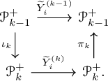
Equivalently, we have
 $$ \begin{align*} \pi_{k}\widetilde{Y}_i^{(k)} f=\widetilde{Y}_i^{(k-1)} f \end{align*} $$
for all $f\in \mathscr {P}_{k-1}^{+}$
.
$f\in \mathscr {P}_{k-1}^{+}$
.
Proof. Note that $\operatorname {\mathrm {pr}}_1\omega ^{-1}_{k}=\omega ^{-1}_{k}\operatorname {\mathrm {pr}}_k$
. For any
$\operatorname {\mathrm {pr}}_1\omega ^{-1}_{k}=\omega ^{-1}_{k}\operatorname {\mathrm {pr}}_k$
. For any $f\in \mathscr {P}_{k-1}^{+}$
, we have
$f\in \mathscr {P}_{k-1}^{+}$
, we have
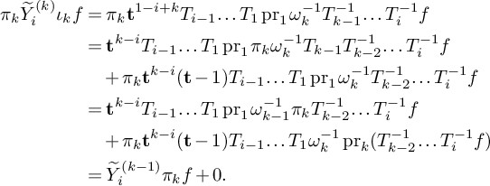 $$ \begin{align*} \pi_{k}\widetilde{Y}_i^{(k)}\iota_k f&=\pi_{k}\textbf{t}^{1-i+k}T_{i-1} \dots T_{1} \operatorname{\mathrm{pr}}_1\omega^{-1}_{k}T_{k-1}^{-1}\dots T_i^{-1}f\\ &=\textbf{t}^{k-i}T_{i-1} \dots T_{1}\operatorname{\mathrm{pr}}_1\pi_{k}\omega^{-1}_{k}T_{k-1}T_{k-2}^{-1}\dots T_i^{-1}f\\&\quad+\pi_{k}\textbf{t}^{k-i}(\textbf{t}-1)T_{i-1} \dots T_{1}\operatorname{\mathrm{pr}}_1\omega^{-1}_{k}T_{k-2}^{-1}\dots T_i^{-1}f\\ &=\textbf{t}^{k-i}T_{i-1} \dots T_{1}\operatorname{\mathrm{pr}}_1\omega^{-1}_{k-1}\pi_{k}T_{k-2}^{-1}\dots T_i^{-1}f\\&\quad+\pi_{k}\textbf{t}^{k-i}(\textbf{t}-1)T_{i-1} \dots T_{1}\omega^{-1}_{k}\operatorname{\mathrm{pr}}_k(T_{k-2}^{-1}\dots T_i^{-1}f)\\ &=\widetilde{Y}_i^{(k-1)}\pi_{k}f+0. \end{align*} $$
For the third equality, we used equation (6.2).
As an immediate consequence, we obtain the following.
Proposition 6.11. For any $i\geq 1$
, the sequence of operators
$i\geq 1$
, the sequence of operators $(\widetilde {Y}_i^{(k)})_{k\geq 2}$
induces a map
$(\widetilde {Y}_i^{(k)})_{k\geq 2}$
induces a map
 $$ \begin{align*} \widetilde{Y}_i^{(\infty)}: \lim_{{\longrightarrow}} \mathscr{P}_k^+\to \mathscr{P}_{\infty}^{+} \end{align*} $$
such that $\Pi _k \widetilde {Y}_i^{(\infty )} I_k=\widetilde {Y}_i^{(k)}$
for all
$\Pi _k \widetilde {Y}_i^{(\infty )} I_k=\widetilde {Y}_i^{(k)}$
for all $k\geq i$
,
$k\geq i$
, $k\geq 2$
.
$k\geq 2$
.
Proof. Fix $n\geq i$
, and denote by
$n\geq i$
, and denote by $\iota _{n,k}: \mathscr {P}_n^+\to \mathscr {P}_k^+$
,
$\iota _{n,k}: \mathscr {P}_n^+\to \mathscr {P}_k^+$
, $n\leq k$
, the canonical inclusion. By Lemma 6.10, the sequence of maps
$n\leq k$
, the canonical inclusion. By Lemma 6.10, the sequence of maps $\widetilde {Y}_i^{(k)} \iota _{n,k}: \mathscr {P}_n^+\to \mathscr {P}_k^+$
,
$\widetilde {Y}_i^{(k)} \iota _{n,k}: \mathscr {P}_n^+\to \mathscr {P}_k^+$
, $k\geq n,i$
is compatible with the structure maps
$k\geq n,i$
is compatible with the structure maps $\pi _k$
. Therefore, they induce a morphism
$\pi _k$
. Therefore, they induce a morphism
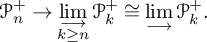 $$ \begin{align*} \mathscr{P}_n^+\to \lim_{\substack{\longrightarrow \\ k\geq n}} \mathscr{P}_k^+\cong \displaystyle \lim_{{\longrightarrow }} \mathscr{P}_k^+. \end{align*} $$
Furthermore, Lemma 6.10 implies that these maps are compatible with the structure maps $\iota _n$
and therefore induce the desired morphism.
$\iota _n$
and therefore induce the desired morphism.
Example 6.12. To illustrate the construction of the limit operator $\widetilde {Y}_1^{(\infty )}: \displaystyle {\lim _{{\longrightarrow }}} \mathscr {P}_k^+\to \mathscr {P}_{\infty }^{+}$
, let us compute its action on the element
$\widetilde {Y}_1^{(\infty )}: \displaystyle {\lim _{{\longrightarrow }}} \mathscr {P}_k^+\to \mathscr {P}_{\infty }^{+}$
, let us compute its action on the element $x_2^2\in \displaystyle {\lim _{{\longrightarrow }}} \mathscr {P}_k^+$
. A direct computation gives
$x_2^2\in \displaystyle {\lim _{{\longrightarrow }}} \mathscr {P}_k^+$
. A direct computation gives
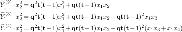 $$ \begin{align*} \widetilde{Y}_1^{(2)}\cdot x_2^2&=\textbf{q}^2 \textbf{t}(\textbf{t}-1)x_1^2+\textbf{q}\textbf{t}(\textbf{t}-1)x_1 x_2\\ \widetilde{Y}_1^{(3)}\cdot x_2^2&=\textbf{q}^2 \textbf{t}(\textbf{t}-1)x_1^2+\textbf{q}\textbf{t}(\textbf{t}-1)x_1 x_2-\textbf{q}\textbf{t}(\textbf{t}-1)^2 x_1x_3\\ \widetilde{Y}_1^{(4)}\cdot x_2^2&=\textbf{q}^2 \textbf{t}(\textbf{t}-1)x_1^2+\textbf{q}\textbf{t}(\textbf{t}-1)x_1 x_2-\textbf{q}\textbf{t}(\textbf{t}-1)^2 (x_1x_3+x_1x_4) \end{align*} $$
and, more generally, for $k\geq 4$
,
$k\geq 4$
,
 $$ \begin{align*} \widetilde{Y}_1^{(k)}\cdot x_2^2=\textbf{q}^2 \textbf{t}(\textbf{t}-1)x_1^2+\textbf{q}\textbf{t}(\textbf{t}-1)x_1 x_2-\textbf{q}\textbf{t}(\textbf{t}-1)^2 (x_1x_3+\cdots x_1x_k). \end{align*} $$
Therefore, the limit operator acts as
 $$ \begin{align*} \widetilde{Y}_1^{(\infty)}\cdot x_2^2=\textbf{q}^2 \textbf{t}(\textbf{t}-1)x_1^2+\textbf{q}\textbf{t}(\textbf{t}-1)x_1 x_2-\textbf{q}\textbf{t}(\textbf{t}-1)^2 x_1 e_1[\mathbf{X}_2]. \end{align*} $$
On the other hand, the action same operator on a nonconstant sequence (e.g., one that converges to a nontrivial almost symmetric function) shows a slightly different behaviour.
Example 6.13. Let $F[\mathbf {X}]=x_2^2+x_3^2+\cdots =p_2[\mathbf {X}_1]$
, which is the inverse limit of the sequence
$F[\mathbf {X}]=x_2^2+x_3^2+\cdots =p_2[\mathbf {X}_1]$
, which is the inverse limit of the sequence
 $$ \begin{align*} F_{k}=\Pi_k F[\mathbf{X}]=x_2^2+\cdots+x_k^2,~ k\geq 2. \end{align*} $$
We have
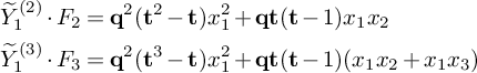 $$ \begin{align*} \widetilde{Y}_1^{(2)}\cdot F_{2}&=\textbf{q}^2(\textbf{t}^2-\textbf{t})x_1^2+\textbf{q}\textbf{t}(\textbf{t}-1)x_1 x_2\\ \widetilde{Y}_1^{(3)}\cdot F_{3}&=\textbf{q}^2(\textbf{t}^3-\textbf{t})x_1^2+\textbf{q}\textbf{t}(\textbf{t}-1)(x_1 x_2+x_1 x_3) \end{align*} $$
and, more generally, for $k\geq 2$
,
$k\geq 2$
,
 $$ \begin{align*} \widetilde{Y}_1^{(k)}\cdot F_{k}=\textbf{q}^2(\textbf{t}^k-\textbf{t})x_1^2+\textbf{q}\textbf{t}(\textbf{t}-1)(x_1 x_2+x_1 x_3+\cdots+x_1x_k). \end{align*} $$
As it can be clearly seen, the sequence $ \widetilde {Y}_1^{(k)}F_{k}$
fails to have an inverse limit because of the contribution of the term
$ \widetilde {Y}_1^{(k)}F_{k}$
fails to have an inverse limit because of the contribution of the term $\textbf {q}^2(\textbf {t}^k-\textbf {t})x_1^2$
.
$\textbf {q}^2(\textbf {t}^k-\textbf {t})x_1^2$
.
As we will see next, the general behaviour of the action of fixed operator on a sequence with inverse limit is no more complicated than the one exhibited in Example 6.13. The operators $W_i^{(k)}$
introduced in the next section formalize this observation.
$W_i^{(k)}$
introduced in the next section formalize this observation.
6.8
We define the $\mathbb {Q}(\textbf {t},\textbf {q})$
-linear operators
$\mathbb {Q}(\textbf {t},\textbf {q})$
-linear operators $\displaystyle W^{(k)}_i: \mathscr {P}_k^+\to \mathscr {P}_{k}^{+}$
,
$\displaystyle W^{(k)}_i: \mathscr {P}_k^+\to \mathscr {P}_{k}^{+}$
, $i\geq 1$
, as follows. Let
$i\geq 1$
, as follows. Let $s\geq 0$
, and let
$s\geq 0$
, and let $i_1<i_2<\dots <i_s\leq k$
and
$i_1<i_2<\dots <i_s\leq k$
and $t_1, \dots , t_s$
be positive integers. We set
$t_1, \dots , t_s$
be positive integers. We set
 $$ \begin{align} W^{(k)}_1(x_{i_1}^{t_{1}}\dots x_{i_s}^{t_{s}})=\begin{cases} 0, & \text{ if } 1=i_1 \text{ or }s=0,\\\\ \ \textbf{t}^{i_s}(1-\textbf{t}^{-1})\textbf{q}^{t_{s}}x_{1}^{t_{s}}x_{i_1}^{t_{1}}\dots x_{i_{s-1}}^{t_{s-1}}, & \text{ if } i_1>1. \end{cases} \end{align} $$
Define
 $$ \begin{align*} W^{(k)}_{i+1}=\textbf{t}^{-1} T_i W^{(k)}_i T_i,\quad 1\leq i\leq k-1. \end{align*} $$
For $1\leq i\leq k$
, we also denote
$1\leq i\leq k$
, we also denote
 $$ \begin{align*} \widetilde{Z}_{i}^{(k)}=\widetilde{Y}_{i}^{(k)}-W_{i}^{(k)}. \end{align*} $$
Lemma 6.14. The following diagram is commutative:
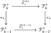
Proof. It is enough to prove the statement for $i=1$
. For any monomial
$i=1$
. For any monomial $f\in \mathscr {P}_{k-1}^{+}$
, we have
$f\in \mathscr {P}_{k-1}^{+}$
, we have
 $$ \begin{align*} \pi_k W_1^{(k)} f =W_1^{(k-1)}\pi_k f \end{align*} $$
and the commutativity of the diagram follows from Lemma 6.10.
Let $f\in x_k \mathscr {P}_{k}^{+}$
be a monomial and
$f\in x_k \mathscr {P}_{k}^{+}$
be a monomial and $g\in \mathscr {P}_{k}^{+}$
. A direct check shows that
$g\in \mathscr {P}_{k}^{+}$
. A direct check shows that
 $$ \begin{align*} \pi_k\omega^{-1}_{k}\operatorname{\mathrm{pr}}_kT_{k-1}^{-1}\operatorname{\mathrm{pr}}_k g \neq 0 \end{align*} $$
only if g is not divisible by $x_{k-1}$
. On the other hand,
$x_{k-1}$
. On the other hand,
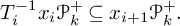 $$ \begin{align*} T_i^{-1} x_i\mathscr{P}_k^+ \subseteq x_{i+1}\mathscr{P}_k^+. \end{align*} $$
Now,
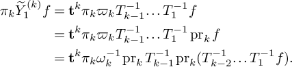 $$ \begin{align*} \pi_k \widetilde{Y}_{1}^{(k)}f&= \textbf{t}^k \pi_k\varpi_k T_{k-1}^{-1}\dots T_{1}^{-1} f\\ &=\textbf{t}^k \pi_k\varpi_k T_{k-1}^{-1}\dots T_{1}^{-1}\operatorname{\mathrm{pr}}_k f\\ &=\textbf{t}^k \pi_k\omega^{-1}_{k}\operatorname{\mathrm{pr}}_kT_{k-1}^{-1}\operatorname{\mathrm{pr}}_k (T_{k-2}^{-1}\dots T_{1}^{-1} f). \end{align*} $$
Based on the previous remarks, $\pi _k \widetilde {Y}_{1}^{(k)}f\neq 0$
unless f is not divisible by
$\pi _k \widetilde {Y}_{1}^{(k)}f\neq 0$
unless f is not divisible by $x_1$
. Furthermore, the only monomial from
$x_1$
. Furthermore, the only monomial from $T_1^{-1}f$
that survives is
$T_1^{-1}f$
that survives is $s_1 f$
. Applying this repeatedly, we obtain
$s_1 f$
. Applying this repeatedly, we obtain
 $$ \begin{align*} \pi_k \widetilde{Y}_{1}^{(k)}f=\textbf{t}^k \pi_k\omega^{-1}_{k}\operatorname{\mathrm{pr}}_kT_{k-1}^{-1}\operatorname{\mathrm{pr}}_k (s_{k-2}\dots s_1 f)=W_{1}^{(k)}f. \end{align*} $$
Therefore, $\pi _k\widetilde {Z}_{i}^{(k)} f=0=\widetilde {Z}_{i}^{(k-1)} \pi _k f$
, as expected.
$\pi _k\widetilde {Z}_{i}^{(k)} f=0=\widetilde {Z}_{i}^{(k-1)} \pi _k f$
, as expected.
As a consequence, we obtain the following.
Proposition 6.15. For any $i\geq 1$
, the sequence of operators
$i\geq 1$
, the sequence of operators $(\widetilde {Z}_i^{(k)})_{k\geq 2}$
induces a map
$(\widetilde {Z}_i^{(k)})_{k\geq 2}$
induces a map
 $$ \begin{align*} \widetilde{Z}_i^{(\infty)}: \mathscr{P}_{\infty}^+\to \mathscr{P}_{\infty}^{+} \end{align*} $$
such that $\Pi _k \widetilde {Z}_i^{(\infty )}=\widetilde {Z}_i^{(k)}$
for all
$\Pi _k \widetilde {Z}_i^{(\infty )}=\widetilde {Z}_i^{(k)}$
for all $k\geq i$
,
$k\geq i$
, $k\geq 2$
.
$k\geq 2$
.
Example 6.16. In continuation of Example 6.12, we illustrate the actions of the operators $W_1^{(k)}$
and
$W_1^{(k)}$
and $\widetilde {Z}_1^{(k)}$
on the constant sequence
$\widetilde {Z}_1^{(k)}$
on the constant sequence $x_2^2$
. We have
$x_2^2$
. We have
 $$ \begin{align*} W_1^{(k)}\cdot x_2^2=\textbf{q}^2 \textbf{t}(\textbf{t}-1)x_1^2 \quad \text{ and }\quad \widetilde{Z}_1^{(k)}\cdot x_2^2=\textbf{q}\textbf{t}(\textbf{t}-1)x_1 x_2-\textbf{q}\textbf{t}(\textbf{t}-1)^2 (x_1x_3+\cdots +x_1x_k),~ k\geq 3. \end{align*} $$
Clearly, both sequences have inverse limit, in particular,
 $$ \begin{align*} \widetilde{Z}_1^{(\infty)}\cdot x_2^2=\textbf{q}\textbf{t}(\textbf{t}-1)x_1 x_2-\textbf{q}\textbf{t}(\textbf{t}-1)^2 x_1 e_1[\mathbf{X}_2]. \end{align*} $$
Example 6.17. In continuation of Example 6.13, we illustrate the actions of the operators $W_1^{(k)}$
and
$W_1^{(k)}$
and $Z_1^{(k)}$
on the sequence
$Z_1^{(k)}$
on the sequence $F_k=x^2_2+\cdots +x^2_k$
. We have
$F_k=x^2_2+\cdots +x^2_k$
. We have
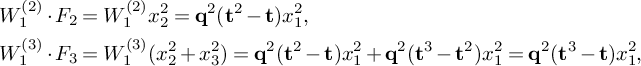 $$ \begin{align*} W_1^{(2)}\cdot F_{2}&=W_1^{(2)}x_2^2=\textbf{q}^2(\textbf{t}^2-\textbf{t})x_1^2,\\ W_1^{(3)}\cdot F_{3}&=W_1^{(3)}(x_2^2+x_3^2)=\textbf{q}^2(\textbf{t}^2-\textbf{t})x_1^2+\textbf{q}^2(\textbf{t}^3-\textbf{t}^2)x_1^2= \textbf{q}^2(\textbf{t}^3-\textbf{t})x_1^2, \end{align*} $$
and, more generally, for $k\geq 2$
,
$k\geq 2$
,
 $$ \begin{align*} W_1^{(k)}\cdot F_{k}=\textbf{q}^2(\textbf{t}^k-\textbf{t})x_1^2. \end{align*} $$
Furthermore,
 $$ \begin{align*} \widetilde{Z}_1^{(k)} \cdot F_{k}=\widetilde{Y}_1^{(k)}\cdot F_{k}-W_1^{(k)}\cdot F_{k}=\textbf{q}\textbf{t}(\textbf{t}-1)(x_1 x_2+x_1 x_3+ \ldots + x_1x_k), \end{align*} $$
which can be seen to have inverse limit. Therefore,
 $$ \begin{align*} \widetilde{Z}_1^{(\infty)}\cdot F[\mathbf{X}]=\textbf{q}\textbf{t}(\textbf{t}-1)x_1 e_1[\mathbf{X}_1]. \end{align*} $$
6.9
Proposition 6.15 motivates the concept of limit we define as follows; We emphasize that this concept of limit depends intrinsically on the structure of the subspace $\mathscr {P}_{\mathrm {as}}^+\subset \mathscr {P}^+_{\infty }$
.
$\mathscr {P}_{\mathrm {as}}^+\subset \mathscr {P}^+_{\infty }$
.
Let $R(\textbf {t},\textbf {q})=A(\textbf {t},\textbf {q})/B(\textbf {t},\textbf {q})\in \mathbb {Q}(\textbf {t},\textbf {q})$
, with
$R(\textbf {t},\textbf {q})=A(\textbf {t},\textbf {q})/B(\textbf {t},\textbf {q})\in \mathbb {Q}(\textbf {t},\textbf {q})$
, with $A(\textbf {t},\textbf {q}),~B(\textbf {t},\textbf {q})\in \mathbb {Q}[\textbf {t},\textbf {q}]$
. The order of vanishing at
$A(\textbf {t},\textbf {q}),~B(\textbf {t},\textbf {q})\in \mathbb {Q}[\textbf {t},\textbf {q}]$
. The order of vanishing at $\textbf {t}=0$
for
$\textbf {t}=0$
for $R(\textbf {t},\textbf {q})$
, denoted by
$R(\textbf {t},\textbf {q})$
, denoted by
 $$ \begin{align*} \operatorname{\mathrm{ord}} R(\textbf{t},\textbf{q}), \end{align*} $$
is the difference between the order of vanishing at $\textbf {t}=0$
for
$\textbf {t}=0$
for $A(\textbf {t},\textbf {q})$
and
$A(\textbf {t},\textbf {q})$
and $B(\textbf {t},\textbf {q})$
.
$B(\textbf {t},\textbf {q})$
.
We say that the sequence $(a_n)_{n\geq 1}\subset \mathbb {Q}(\textbf {t},\textbf {q})$
converges to
$(a_n)_{n\geq 1}\subset \mathbb {Q}(\textbf {t},\textbf {q})$
converges to $0$
if the sequence
$0$
if the sequence $(\operatorname {\mathrm {ord}} a_n)_{n\geq 1}\subset \mathbb Z$
converges to
$(\operatorname {\mathrm {ord}} a_n)_{n\geq 1}\subset \mathbb Z$
converges to $+\infty $
. We say that the sequence
$+\infty $
. We say that the sequence $(a_n)_{n\geq 1}\subset \mathbb {Q}(\textbf {t},\textbf {q})$
converges to a if
$(a_n)_{n\geq 1}\subset \mathbb {Q}(\textbf {t},\textbf {q})$
converges to a if $(a_n-a)_{n\geq 1}$
converges to
$(a_n-a)_{n\geq 1}$
converges to $0$
. We write,
$0$
. We write,
 $$ \begin{align*} \lim_{n\to \infty} a_n=a. \end{align*} $$
Definition 6.18. Let $(f_k)_{k\geq 1}$
be a sequence with
$(f_k)_{k\geq 1}$
be a sequence with $f_k\in \mathscr {P}^+_k$
. We say that the sequence is convergent if there exists
$f_k\in \mathscr {P}^+_k$
. We say that the sequence is convergent if there exists $N\geq 1$
and sequences
$N\geq 1$
and sequences $(h_k)_{k\geq 1}$
,
$(h_k)_{k\geq 1}$
, $(g_{i,k})_{k\geq 1}$
,
$(g_{i,k})_{k\geq 1}$
, $i\leq N$
,
$i\leq N$
, $h_k, ~g_{i, k}\in \mathscr {P}^+_k$
and
$h_k, ~g_{i, k}\in \mathscr {P}^+_k$
and $(a_{i, k})_{k\leq 1}$
,
$(a_{i, k})_{k\leq 1}$
, $i\leq N$
,
$i\leq N$
, $a_{i, k}\in \mathbb {Q}(\textbf {t},\textbf {q})$
such that
$a_{i, k}\in \mathbb {Q}(\textbf {t},\textbf {q})$
such that
-
a) For any
$k\geq 1$
, we have
$f_k=h_k+\sum _{i=1}^N a_{i, k} g_{i, k}$
; -
b) For any
$i\leq N$
,
$k\geq 2$
,
$\pi _k(g_{i, k})=g_{i, k-1}$
and
$\pi _k(h_{k})=h_{k-1}$
. We denote by the sequence
$$ \begin{align*} \displaystyle g_i=\lim_{k\to \infty} g_{i,k}\quad \text{and}\quad \displaystyle h=\lim_{k\to \infty} h_{k} \end{align*} $$
$(g_{i,k})_{k\geq 1}$
and, respectively,
$(h_{k})_{k\geq 1}$
as elements of
$\mathscr {P}_{\infty }^+$
. We require that
$g_i\in \mathscr {P}_{\mathrm {as}}^+$
.
-
c) For any
$i\leq N$
, the sequence
$(a_{i, k})_{k\geq 1}$
is convergent. We denote
$\displaystyle a_i=\lim _{k\to \infty }(a_{i, k})$
.


If the sequence $(f_k)_{k\geq 1}$
is convergent, we define its limit as
$(f_k)_{k\geq 1}$
is convergent, we define its limit as
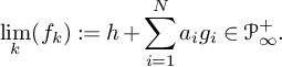 $$ \begin{align*} \lim_k(f_k):=h+ \sum_{i=1}^N a_i g_i\in\mathscr{P}_{\infty}^+. \end{align*} $$
Example 6.19. The sequence
 $$ \begin{align*} f_k=(1+\textbf{t}+\ldots +\textbf{t}^k)e_i[\overline{\mathbf{X}}_{k}], \end{align*} $$
has the limit
 $$ \begin{align*} \lim_k f_k=\frac{1}{1-\textbf{t}}e_i[\mathbf{X}]. \end{align*} $$
The sequence
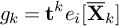 $$ \begin{align*} g_k=\textbf{t}^k e_i[\overline{\mathbf{X}}_{k}] \end{align*} $$
has limit $0$
.
$0$
.
We show that the limit of a sequence does not depend on the choice of the auxiliary sequences in Definition 6.18.
Proposition 6.20. The concept of limit is well-defined.
Proof. It suffices to show that the limit of the constant sequence $0$
is zero, regardless of the auxiliary sequences in Definition 6.18. Consider sequences
$0$
is zero, regardless of the auxiliary sequences in Definition 6.18. Consider sequences $(c_{i,k})_{k\geq 1}$
and
$(c_{i,k})_{k\geq 1}$
and $(q_{i,k})_{k\geq 1}$
such that
$(q_{i,k})_{k\geq 1}$
such that
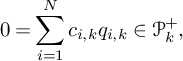 $$ \begin{align*} 0=\sum_{i=1}^{N}c_{i,k}q_{i,k}\in \mathscr{P}_{k}^{+}, \end{align*} $$
and
 $$ \begin{align*} \lim_{k\rightarrow\infty}c_{i,k}=c_i\in \mathbb{Q}(\textbf{t},\textbf{q}),\ \lim_{k\rightarrow\infty}q_{i,k}=q_i\in\mathscr{P}_{\mathrm{as}}^{+}. \end{align*} $$
We need to show that $\sum _{i=1}^N c_iq_i=0$
.
$\sum _{i=1}^N c_iq_i=0$
.
Without loss of generality, we assume that $q_1,\ldots ,q_N$
are
$q_1,\ldots ,q_N$
are $\mathbb {Q}$
-linearly independent. Indeed, any linear relation between
$\mathbb {Q}$
-linearly independent. Indeed, any linear relation between $q_1,\ldots ,q_N$
must also hold for
$q_1,\ldots ,q_N$
must also hold for $q_{1,k},\ldots ,q_{N,k}$
for all k. We can therefore substitute one of them, say
$q_{1,k},\ldots ,q_{N,k}$
for all k. We can therefore substitute one of them, say $q_{1,k}$
, with the same
$q_{1,k}$
, with the same $\mathbb {Q}$
-linear combination of
$\mathbb {Q}$
-linear combination of $q_{2,k},\ldots ,q_{N,k}$
for all k. It is clear that the conclusion does not change after such a substitution.
$q_{2,k},\ldots ,q_{N,k}$
for all k. It is clear that the conclusion does not change after such a substitution.
Recall that each $q_i\in \mathscr {P}_{\mathrm {as}}^{+}$
. We can find
$q_i\in \mathscr {P}_{\mathrm {as}}^{+}$
. We can find $n\geq 1$
such that
$n\geq 1$
such that $q_i\in \mathscr {P}(n)$
for all
$q_i\in \mathscr {P}(n)$
for all $1\leq i\leq N$
. For the same reason as before, without loss of generality, we can assume that
$1\leq i\leq N$
. For the same reason as before, without loss of generality, we can assume that
 $$ \begin{align*} q_i= f_i(x_1,\ldots ,x_n)e_{\alpha_i}[\mathbf{X}_{n}], \end{align*} $$
where
 $$ \begin{align*} \alpha_i=(\alpha_{i,1}\geq\dots \geq\alpha_{i,s_i}), \quad 1\leq i\leq N \end{align*} $$
are distinct partitions. Let
 $$ \begin{align*} M=\max_{1\leq i\leq N}\alpha_{i,1}. \end{align*} $$
For any $k>M+n$
, we claim that
$k>M+n$
, we claim that $q_{1,k},\ldots ,q_{N,k}$
are also
$q_{1,k},\ldots ,q_{N,k}$
are also $\mathbb {Q}$
-linear independent. Indeed, if we have a linear relation
$\mathbb {Q}$
-linear independent. Indeed, if we have a linear relation
 $$ \begin{align*} \sum_{i=1}^{N}a_i f_i(x_1,\ldots ,x_n)e_{\alpha_i}[x_{n+1},\ldots ,x_{k}]=0 \end{align*} $$
for some $a_i\in \mathbb {Q}$
, then, for any evaluation at
$a_i\in \mathbb {Q}$
, then, for any evaluation at $x_1=b_1,\ldots ,x_n=b_n,$
we have
$x_1=b_1,\ldots ,x_n=b_n,$
we have
 $$ \begin{align*} \sum_{i=1}^{N}a_i f_i(b_1,\ldots ,b_n)e_{\alpha_i}[x_{n+1},\ldots ,x_{k}]=0. \end{align*} $$
Note that, because $k-n>M$
and the partitions
$k-n>M$
and the partitions $\alpha _i$
are distinct, the symmetric functions
$\alpha _i$
are distinct, the symmetric functions $e_{\alpha _i}[\mathbf {X}_{n}]$
are linearly independent. Therefore, for all
$e_{\alpha _i}[\mathbf {X}_{n}]$
are linearly independent. Therefore, for all $1\leq i\leq N$
,
$1\leq i\leq N$
,
 $$ \begin{align*} a_i f_i(b_1,\ldots ,b_n)=0. \end{align*} $$
Since $f_i$
are polynomials in finitely many variables, we obtain, for all
$f_i$
are polynomials in finitely many variables, we obtain, for all $1\leq i\leq N$
,
$1\leq i\leq N$
,
 $$ \begin{align*} a_i f_i(x_1,\ldots ,x_n)=0, \end{align*} $$
which is a contradiction. Therefore, for k large enough, we have that $q_{1,k},\ldots ,q_{N,k}$
are
$q_{1,k},\ldots ,q_{N,k}$
are $\mathbb {Q}$
-linear independent.
$\mathbb {Q}$
-linear independent.
We can now prove that for k large enough, all $c_{i,k}$
will necessarily be
$c_{i,k}$
will necessarily be $0$
. Indeed, from the hypothesis we have
$0$
. Indeed, from the hypothesis we have
 $$ \begin{align*} 0=\sum_{i=1}^{N}c_{i,k}q_{i,k}. \end{align*} $$
By multiplying both sides the common denominator of $c_{i,k}$
we may assume all
$c_{i,k}$
we may assume all $c_{i,k}$
are polynomials in two variables
$c_{i,k}$
are polynomials in two variables $\textbf {t},\textbf {q}$
. Again, for any evaluation
$\textbf {t},\textbf {q}$
. Again, for any evaluation $\textbf {q}=a,\textbf {t}=b$
, we have
$\textbf {q}=a,\textbf {t}=b$
, we have
 $$ \begin{align*} 0=\sum_{i=1}^{N}c_{i,k}(a,b)q_{i,k}. \end{align*} $$
But we already now $q_{1,k},\ldots ,q_{N,k}$
are
$q_{1,k},\ldots ,q_{N,k}$
are $\mathbb {Q}$
-linear independent for k large enough. Hence, it forces
$\mathbb {Q}$
-linear independent for k large enough. Hence, it forces $c_{i,k}(a,b)=0$
for all i. Again, this implies that
$c_{i,k}(a,b)=0$
for all i. Again, this implies that $c_{i,k}(\textbf {t},\textbf {q})=0$
,
$c_{i,k}(\textbf {t},\textbf {q})=0$
, $1\leq i\leq N$
.
$1\leq i\leq N$
.
6.10
For later use, we record the following result. To set the notation, assume that $A_k:\mathscr {P}_k^+\to \mathscr {P}_k^+$
,
$A_k:\mathscr {P}_k^+\to \mathscr {P}_k^+$
, $k\geq 1$
, is a sequence of operators with the following property: For any
$k\geq 1$
, is a sequence of operators with the following property: For any $f\in \mathscr {P}_{\mathrm {as}}^+$
, the sequence
$f\in \mathscr {P}_{\mathrm {as}}^+$
, the sequence $(A_k \Pi _k f)_{k\geq 1}$
converges to an element of
$(A_k \Pi _k f)_{k\geq 1}$
converges to an element of $\mathscr {P}_{\mathrm {as}}^+$
. Let
$\mathscr {P}_{\mathrm {as}}^+$
. Let ${A}$
be the operator
${A}$
be the operator
 $$ \begin{align*} A: \mathscr{P}_{\mathrm{as}}^+\to \mathscr{P}_{\mathrm{as}}^+,\quad f\mapsto \lim_k {A}_k \Pi_k f. \end{align*} $$
We refer to A as the limit operator of the sequence $(A_k)_{k\geq 1}$
.
$(A_k)_{k\geq 1}$
.
Proposition 6.21. Let $(f_k)_{k\geq 1}$
,
$(f_k)_{k\geq 1}$
, $f_k\in \mathscr {P}_k^+$
be a convergent sequence such that
$f_k\in \mathscr {P}_k^+$
be a convergent sequence such that $f=\lim _{k} f_k\in \mathscr {P}_{\mathrm {as}}^+$
. Then, with the notation above, we have
$f=\lim _{k} f_k\in \mathscr {P}_{\mathrm {as}}^+$
. Then, with the notation above, we have
 $$ \begin{align*} A f=\lim_{k}A_{k} f_k. \end{align*} $$
Proof. By replacing $f_k$
with
$f_k$
with $f_k-\Pi _k$
, it is enough to prove the statement for the case
$f_k-\Pi _k$
, it is enough to prove the statement for the case $f=0$
. Assume that
$f=0$
. Assume that $f=0$
. In this case, there exist sequences
$f=0$
. In this case, there exist sequences $(c_{i,k})_{k\geq 1}$
and
$(c_{i,k})_{k\geq 1}$
and $(q_{i,k})_{k\geq 1}$
as in Definition 6.18 such that
$(q_{i,k})_{k\geq 1}$
as in Definition 6.18 such that
 $$ \begin{align*} f_k=\sum_{i=1}^{N}c_{i,k}q_{i,k}\in \mathscr{P}_{k}^{+}, \end{align*} $$
with
 $$ \begin{align*} \lim_{k\rightarrow\infty}c_{i,k}=c_i\in \mathbb{Q}(\textbf{t},\textbf{q}),\ \lim_{k\rightarrow\infty}q_{i,k}=q_i\in\mathscr{P}_{\mathrm{as}}^{+}. \end{align*} $$
For each i such that $c_i\neq 0$
, we may replace
$c_i\neq 0$
, we may replace $c_{i,k}$
with
$c_{i,k}$
with $c_{i,k}/c_i$
and
$c_{i,k}/c_i$
and $q_{i,k}$
with
$q_{i,k}$
with $c_i q_{i,k}$
. This allows us to assume that
$c_i q_{i,k}$
. This allows us to assume that $c_i\in \{0,1\}$
. Without loss of generality, we assume that
$c_i\in \{0,1\}$
. Without loss of generality, we assume that $q_1,\ldots ,q_N$
are
$q_1,\ldots ,q_N$
are $\mathbb {Q}$
-linearly independent. Indeed, any linear relation between
$\mathbb {Q}$
-linearly independent. Indeed, any linear relation between $q_1,\ldots ,q_N$
must also hold for
$q_1,\ldots ,q_N$
must also hold for $q_{1,k},\ldots ,q_{N,k}$
, for all k. We can therefore substitute one of them, say
$q_{1,k},\ldots ,q_{N,k}$
, for all k. We can therefore substitute one of them, say $q_{1,k}$
, with the same
$q_{1,k}$
, with the same $\mathbb {Q}$
-linear combination of
$\mathbb {Q}$
-linear combination of $q_{2,k},\ldots ,q_{N,k}$
for all k. It is clear that the conclusion does not change after such a substitution. It is now clear that for all i we have
$q_{2,k},\ldots ,q_{N,k}$
for all k. It is clear that the conclusion does not change after such a substitution. It is now clear that for all i we have $c_i=0$
.
$c_i=0$
.
For any $k\geq 1$
,
$k\geq 1$
,
 $$ \begin{align*} A_k f_k=\sum_{i=1}^N c_{i,k} A_k q_{i,k}=\sum_{i=1}^N c_{i,k} A_k \Pi_k q_i. \end{align*} $$
Since $\displaystyle \lim _{k\rightarrow \infty }A_k \Pi _k q_i=A q_i\in \mathscr {P}_{\mathrm {as}}^{+}$
, we have, by Definition 6.18,
$\displaystyle \lim _{k\rightarrow \infty }A_k \Pi _k q_i=A q_i\in \mathscr {P}_{\mathrm {as}}^{+}$
, we have, by Definition 6.18,
 $$ \begin{align*} \lim_k A_k f_k=\sum_{i=1}^N c_{i,k} A q_i=0. \end{align*} $$
This is precisely our claim.
This result can be interpreted as a property of continuity for the operator A. Let $(B_k)_{k\geq 1}$
be another sequence of operators with the same property as
$(B_k)_{k\geq 1}$
be another sequence of operators with the same property as $(A_k)_{k\geq 1}$
and denote by
$(A_k)_{k\geq 1}$
and denote by $B: \mathscr {P}_{\mathrm {as}}^+\to \mathscr {P}_{\mathrm {as}}^+$
the corresponding limit operator.
$B: \mathscr {P}_{\mathrm {as}}^+\to \mathscr {P}_{\mathrm {as}}^+$
the corresponding limit operator.
Corollary 6.22. With the notation above, the operator $AB$
is the limit of the sequence
$AB$
is the limit of the sequence $(A_kB_k)_{k\geq 1}$
.
$(A_kB_k)_{k\geq 1}$
.
Proof. Let $f\in \mathscr {P}_{\mathrm {as}}^+$
. Since
$f\in \mathscr {P}_{\mathrm {as}}^+$
. Since $\displaystyle \lim _k B_k\Pi _kf=B f\in \mathscr {P}_{\mathrm {as}}^+$
, we can apply Proposition 6.21 to obtain
$\displaystyle \lim _k B_k\Pi _kf=B f\in \mathscr {P}_{\mathrm {as}}^+$
, we can apply Proposition 6.21 to obtain
 $$ \begin{align*} \lim_k A_k B_k \Pi_k f=A B f \in \mathscr{P}_{\mathrm{as}}^+, \end{align*} $$
which proves our claim.
6.11
Let us examine the following situation.
Lemma 6.23. Let $f\in \mathscr {P}_{\mathrm {as}}^+$
and
$f\in \mathscr {P}_{\mathrm {as}}^+$
and $i\geq 1$
. The sequence
$i\geq 1$
. The sequence $W_i^{(k)} \Pi _k f$
converges. We define
$W_i^{(k)} \Pi _k f$
converges. We define
 $$ \begin{align*} W^{(\infty)}_i: \mathscr{P}_{\mathrm{as}}^+\to \mathscr{P}_{\infty}^+,\quad W^{(\infty)}_i f=\lim_{k} W_i^{(k)}\Pi_k f\in \mathscr{P}_{\infty}^{+}. \end{align*} $$
Proof. It is enough to prove our claim for $W_1$
and
$W_1$
and $f=g(x_1,\dots ,x_n)m_{\alpha }[\mathbf {X}_n]$
for some
$f=g(x_1,\dots ,x_n)m_{\alpha }[\mathbf {X}_n]$
for some $n\geq 1$
, where g is a monomial and
$n\geq 1$
, where g is a monomial and $m_{\alpha }$
is the monomial symmetric function in the indicated alphabet. If
$m_{\alpha }$
is the monomial symmetric function in the indicated alphabet. If $x_1$
divides g, then
$x_1$
divides g, then $W_1f=0$
. We assume that
$W_1f=0$
. We assume that $x_1$
does not divide g.
$x_1$
does not divide g.
We denote by $\ell (\alpha )$
the length of the partition
$\ell (\alpha )$
the length of the partition $\alpha $
. Of course, for any
$\alpha $
. Of course, for any $k\geq n+\ell (\alpha )$
, we have
$k\geq n+\ell (\alpha )$
, we have
 $$ \begin{align*} \Pi_k m_{\alpha}[\mathbf{X}_n]=m_{\alpha}[x_{n+1},\dots ,x_k]. \end{align*} $$
If $k\geq n+\ell (\alpha )$
, denote by
$k\geq n+\ell (\alpha )$
, denote by $a_1,\dots , a_s$
the distinct parts of
$a_1,\dots , a_s$
the distinct parts of $\alpha $
. Let
$\alpha $
. Let $\beta _i$
,
$\beta _i$
, $1\leq i\leq s$
the partition obtained by eliminating one part of size
$1\leq i\leq s$
the partition obtained by eliminating one part of size $a_i$
from
$a_i$
from $\alpha $
. Then,
$\alpha $
. Then,
 $$ \begin{align*} m_{\alpha}[x_{n+1},\dots,x_k]=\sum_{i=1}^s \sum_{j=n+\ell(\alpha)}^k m_{\beta_i}[x_{n+1},\dots, x_{j-1}] x_j^{a_i}. \end{align*} $$
Therefore, we have
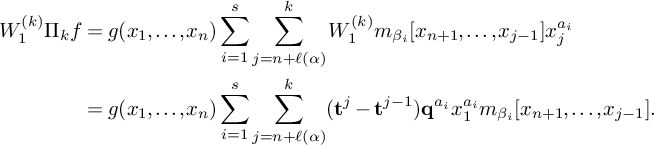 $$ \begin{align*} W_{1}^{(k)}\Pi_k f &=g(x_1,\dots,x_n) \sum_{i=1}^s \sum_{j=n+\ell(\alpha)}^k W_1^{(k)} m_{\beta_i}[x_{n+1},\dots, x_{j-1}] x_j^{a_i}\\ &=g(x_1,\dots,x_n) \sum_{i=1}^s \sum_{j=n+\ell(\alpha)}^k (\textbf{t}^j-\textbf{t}^{j-1})\textbf{q}^{a_i} x_1^{a_i} m_{\beta_i}[x_{n+1},\dots, x_{j-1}]. \end{align*} $$
For a monomial $m=x_{i_1}^{\eta _1}\cdots x_{i_M}^{\eta _M}$
,
$m=x_{i_1}^{\eta _1}\cdots x_{i_M}^{\eta _M}$
, $n<i_1<\dots <i_M$
,
$n<i_1<\dots <i_M$
, $\eta _1,\dots ,\eta _M\geq 1$
, we denote
$\eta _1,\dots ,\eta _M\geq 1$
, we denote $\ell (m)=i_M$
and we write
$\ell (m)=i_M$
and we write $m\in [\beta ]$
if
$m\in [\beta ]$
if $(\eta _1,\dots , \eta _M)$
is a permutation of
$(\eta _1,\dots , \eta _M)$
is a permutation of $\beta $
and we write
$\beta $
and we write $m\in [\beta ]_k$
if
$m\in [\beta ]_k$
if $m\in [\beta ]$
and
$m\in [\beta ]$
and $\ell (m)\leq k$
. With this notation, we have
$\ell (m)\leq k$
. With this notation, we have
 $$ \begin{align*} W_{1}^{(k)}\Pi_k f &=g(x_1,\dots,x_n) \sum_{i=1}^s \sum_{m\in [\beta_i]_k} (\textbf{t}^k-\textbf{t}^{\ell(m)})\textbf{q}^{a_i} x_1^{a_i} m\\ &= g(x_1,\dots,x_n)\left(\sum_{i=1}^s \textbf{t}^k \textbf{q}^{a_i} x_1^{a_i} m_{\beta_i}[x_{n+1},\dots,x_k] -\sum_{i=1}^s \textbf{q}^{a_i} x_1^{a_i} \sum_{m\in [\beta_i]_k} \textbf{t}^{\ell(m)} m \right) \end{align*} $$
According to Definition 6.18,
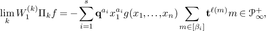 $$ \begin{align*} \lim_k W_{1}^{(k)}\Pi_k f = - \sum_{i=1}^s \textbf{q}^{a_i} x_1^{a_i} g(x_1,\dots,x_n) \sum_{m\in [\beta_i]} \textbf{t}^{\ell(m)} m \in \mathscr{P}_{\infty}^+, \end{align*} $$
which proves our claim.
Example 6.24. The sequence $W_1^{(k)}(x_2^2+\cdots +x_k^2)$
from Example 6.17 has limit
$W_1^{(k)}(x_2^2+\cdots +x_k^2)$
from Example 6.17 has limit $-\textbf {q}^2\textbf {t} x_1^2$
.
$-\textbf {q}^2\textbf {t} x_1^2$
.
6.12
We can now prove the following.
Proposition 6.25. Let $f\in \mathscr {P}_{\mathrm {as}}^+$
and
$f\in \mathscr {P}_{\mathrm {as}}^+$
and $i\geq 1$
. The sequence
$i\geq 1$
. The sequence $\widetilde {Y}_i^{(k)} \Pi _k f$
converges. We define
$\widetilde {Y}_i^{(k)} \Pi _k f$
converges. We define
 $$ \begin{align*} \mathscr{Y}_i: \mathscr{P}_{\mathrm{as}}^+\to \mathscr{P}_{\infty}^+,\quad \mathscr{Y}_i f=\lim_{k} \widetilde{Y}_i^{(k)}\Pi_k f\in \mathscr{P}_{\infty}^{+}. \end{align*} $$
Proof. Straightforward from Proposition 6.15 and Lemma 6.23. More precisely, $\mathscr {Y}_i=\widetilde {Z}^{(\infty )}_i+W^{(\infty )}_i$
.
$\mathscr {Y}_i=\widetilde {Z}^{(\infty )}_i+W^{(\infty )}_i$
.
Example 6.26. In continuation of Examples 6.13 and 6.17, we have
 $$ \begin{align*} \mathscr{Y}_1 \cdot p_2[\mathbf{X}_1]=-\textbf{q}^2 \textbf{t} x_1^2+\textbf{q}\textbf{t}(\textbf{t}-1)x_1 e_1[\mathbf{X}_1]. \end{align*} $$
As it can be seen, $p_2[\mathbf {X}_1]$
and
$p_2[\mathbf {X}_1]$
and $\mathscr {Y}_1 \cdot p_2[\mathbf {X}_1]$
are elements of
$\mathscr {Y}_1 \cdot p_2[\mathbf {X}_1]$
are elements of $\mathscr {P}(1)^+$
.
$\mathscr {P}(1)^+$
.
Also, from Examples 6.12 and 6.16 we have
 $$ \begin{align*} \mathscr{Y}_1 \cdot x_2^2=\textbf{q}^2 \textbf{t}(\textbf{t}-1)x_1^2+\textbf{q}\textbf{t}(\textbf{t}-1)x_1 x_2-\textbf{q}\textbf{t}(\textbf{t}-1)^2 x_1 e_1[\mathbf{X}_2]. \end{align*} $$
In this case, $x_2^2$
and
$x_2^2$
and $\mathscr {Y}_1 x_2^2$
are elements of
$\mathscr {Y}_1 x_2^2$
are elements of $\mathscr {P}(2)^+$
.
$\mathscr {P}(2)^+$
.
It turns out that the image of $\mathscr {Y}_i$
is contained in
$\mathscr {Y}_i$
is contained in $\mathscr {P}_{\mathrm {as}}^+$
. We will use the following result.
$\mathscr {P}_{\mathrm {as}}^+$
. We will use the following result.
Lemma 6.27. Let $f\in \mathbb {Q}(\textbf {t},\textbf {q})[x_{k+1},x_{k+2},\dots ]$
be a polynomial satisfying
$f\in \mathbb {Q}(\textbf {t},\textbf {q})[x_{k+1},x_{k+2},\dots ]$
be a polynomial satisfying
 $$ \begin{align*} T_i f=f,\quad \textrm{ for }k+1\leq i\leq k+m. \end{align*} $$
Let $g=T_{k+m}^{-1}\dots T_{k+1}^{-1}T_k^{-1}(x_{k}^{s}f)$
for some
$g=T_{k+m}^{-1}\dots T_{k+1}^{-1}T_k^{-1}(x_{k}^{s}f)$
for some $s\geq 0$
. Then,
$s\geq 0$
. Then,
 $$ \begin{align*} T_i g=g \quad \textrm{ for }k\leq i\leq k+m-1. \end{align*} $$
Proof. The claim is a consequence of the braid relations for the elements $T_i$
.
$T_i$
.
Lemma 6.28. $\mathscr {P}(k)^{+}$
is stable under the action of
$\mathscr {P}(k)^{+}$
is stable under the action of $\mathscr {Y}_1$
. Therefore, we have
$\mathscr {Y}_1$
. Therefore, we have
 $$ \begin{align*} \mathscr{Y}_i:\mathscr{P}_{\mathrm{as}}^{+}\rightarrow \mathscr{P}_{\mathrm{as}}^{+}. \end{align*} $$
Proof. Let $f\in \mathscr {P}(k)^{+}$
(recall the definition of
$f\in \mathscr {P}(k)^{+}$
(recall the definition of $\mathscr {P}(k)^{+}$
in §2.6). For any
$\mathscr {P}(k)^{+}$
in §2.6). For any $m>k+1$
, we have
$m>k+1$
, we have
 $$ \begin{align*} \widetilde{Y}_1^{(m)} \Pi_m f=\textbf{t}^{m} \varpi_m T_{m-1}^{-1}\dots T_{1}^{-1}\Pi_m f. \end{align*} $$
Since $f\in \mathscr {P}(k)^{+}$
,
$f\in \mathscr {P}(k)^{+}$
, $\Pi _m f$
is fixed under the action of
$\Pi _m f$
is fixed under the action of $T_{k+1},\dots ,T_{m-1}$
. Now, we have
$T_{k+1},\dots ,T_{m-1}$
. Now, we have
 $$ \begin{align*} \varpi_m T_{m-1}^{-1}\dots T_{1}^{-1}\Pi_m f=\varpi_m T_{m-1}^{-1}\dots T_{k+1}^{-1}T_{k}^{-1}(T_{k-1}^{-1}\dots T_{1}^{-1}\Pi_m f),\end{align*} $$
and we may write
 $$ \begin{align*} T_{k-1}^{-1}\dots T_{1}^{-1}\Pi_m f=\sum_{j} c_j[x_1,\dots ,x_{k-1}]x_{k}^{s_j}f_j \end{align*} $$
as a finite sum, where each $f_j$
is a polynomial in
$f_j$
is a polynomial in $\mathbb {Q}(\textbf {t},\textbf {q})[x_{k+1},x_{k+2},\dots ]$
satisfying
$\mathbb {Q}(\textbf {t},\textbf {q})[x_{k+1},x_{k+2},\dots ]$
satisfying
 $$ \begin{align*} T_i f_j=f_j,\quad \textrm{ for }i=k+1,k+2,\dots ,m-1. \end{align*} $$
Applying Lemma 6.27 for $T_{k-1}^{-1}\dots T_{1}^{-1}\Pi _m f$
, we obtain that
$T_{k-1}^{-1}\dots T_{1}^{-1}\Pi _m f$
, we obtain that $ T_{m-1}^{-1}\dots T_{1}^{-1}\Pi _m f$
is fixed under the action of the elements
$ T_{m-1}^{-1}\dots T_{1}^{-1}\Pi _m f$
is fixed under the action of the elements $T_{k},\dots ,T_{m-2}$
. The relation (6.3) implies that
$T_{k},\dots ,T_{m-2}$
. The relation (6.3) implies that $\varpi _m T_{m-1}^{-1}\dots T_{1}^{-1}\Pi _m f$
is fixed under the action of
$\varpi _m T_{m-1}^{-1}\dots T_{1}^{-1}\Pi _m f$
is fixed under the action of $T_{k+1},\dots ,T_{m-1}$
. Therefore,
$T_{k+1},\dots ,T_{m-1}$
. Therefore, $\widetilde {Y}_1^{(m)} \Pi _m f$
is symmetric in
$\widetilde {Y}_1^{(m)} \Pi _m f$
is symmetric in $x_{k+1},\dots , x_m$
for all
$x_{k+1},\dots , x_m$
for all $m>k+1$
. In conclusion, the limit
$m>k+1$
. In conclusion, the limit
 $$ \begin{align*} \displaystyle \lim_{m} \widetilde{Y}_i^{(m)}\Pi_m f\in \mathscr{P}(k)^+, \end{align*} $$
proving our claim.
We can now state the following.
Proposition 6.29. The space $\mathscr {P}_{\mathrm {as}}^+$
carries an action of the limit operators
$\mathscr {P}_{\mathrm {as}}^+$
carries an action of the limit operators $\mathscr {T}_i, \mathscr {X}_i, \mathscr {Y}_i$
,
$\mathscr {T}_i, \mathscr {X}_i, \mathscr {Y}_i$
, $i\geq 1$
.
$i\geq 1$
.
As we will show in Theorem 6.34, these operators define an action of $\mathscr {H}^+$
on
$\mathscr {H}^+$
on $\mathscr {P}_{\mathrm {as}}^+$
.
$\mathscr {P}_{\mathrm {as}}^+$
.
Remark 6.30. Following up on Remark 6.9, it is important to note that on $x_i\mathscr {P}_{\mathrm {as}}^+$
the action of
$x_i\mathscr {P}_{\mathrm {as}}^+$
the action of $\mathscr {Y}_i$
is the stable limit of the action of the sequence of Cherednik operators
$\mathscr {Y}_i$
is the stable limit of the action of the sequence of Cherednik operators $Y^{(k)}_i\in \mathscr {H}_k$
.
$Y^{(k)}_i\in \mathscr {H}_k$
.
6.13
In fact, we can obtain a more precise description of the action of $\mathscr {Y}_1$
on
$\mathscr {Y}_1$
on $\mathscr {P}(k)^+$
. First, let us record the following technical result. We use the notation in §2.3.
$\mathscr {P}(k)^+$
. First, let us record the following technical result. We use the notation in §2.3.
Lemma 6.31. Let $x_1^{n}\in \mathscr {P}^+_{m+1}$
. Then,
$x_1^{n}\in \mathscr {P}^+_{m+1}$
. Then,
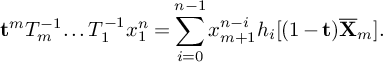 $$ \begin{align*} \textbf{t}^{m}T_{m}^{-1}\ldots T_{1}^{-1}x_1^{n}=\sum_{i=0}^{n-1}x_{m+1}^{n-i}h_i[(1-\textbf{t})\overline{\mathbf{X}}_{m}]. \end{align*} $$
Proof. We will prove the result by induction on m. By direct computation, we obtain
 $$ \begin{align*} T_{1}^{-1}x_1^{n}&=\textbf{t}^{-1}x_2^{n}+(\textbf{t}^{-1}-1)(x_2^{n-1}x_1+x_2^{n-2}x_1^2+\ldots +x_2x_1^{n-1})\\ &=\textbf{t}^{-1}\sum_{i=0}^{n-1}x_{2}^{n-i}h_i[(1-\textbf{t})x_1]. \end{align*} $$
Assume that our claim holds for $m-1$
. Then, we have
$m-1$
. Then, we have
 $$ \begin{align*} \textbf{t}^{m}T_{m}^{-1}\ldots T_{1}^{-1}x_1^{n}&=\textbf{t} T_{m}^{-1}\sum_{i=0}^{n-1}x_{m}^{n-i}h_i[(1-\textbf{t})\overline{\mathbf{X}}_{m-1}]\\ &=\sum_{i=0}^{n-1}\sum_{j=0}^{n-i-1}x_{m+1}^{n-i-j}h_j[(1-\textbf{t})x_m] h_i[(1-\textbf{t})\overline{\mathbf{X}}_{m-1}]\\ &=\sum_{l=0}^{n-1} x_{m+1}^{n-l}\sum_{\substack{i+j=l\\i, j\geq 0}}h_j[(1-\textbf{t})x_m] h_i[(1-\textbf{t})\overline{\mathbf{X}}_{m-1}]\\ &=\sum_{l=0}^{n-1} x_{m+1}^{n-l}h_l[(1-\textbf{t})\overline{\mathbf{X}}_{m}], \end{align*} $$
as expected.
Recall that for all k, the multiplication map $ \mathscr {P}_k^{+}\otimes \operatorname {\mathrm {Sym}}[\mathbf {X}_k] \cong \mathscr {P}(k)^+$
is an algebra isomorphism.
$ \mathscr {P}_k^{+}\otimes \operatorname {\mathrm {Sym}}[\mathbf {X}_k] \cong \mathscr {P}(k)^+$
is an algebra isomorphism.
Proposition 6.32. Let $n\geq 0$
,
$n\geq 0$
, $f(x_1,\dots ,x_{k-1})\in \mathscr {P}_{k-1}^{+}$
, and
$f(x_1,\dots ,x_{k-1})\in \mathscr {P}_{k-1}^{+}$
, and $G[\mathbf {X}_{k-1}]\in \operatorname {\mathrm {Sym}}[\mathbf {X}_{k-1}]$
. We regard
$G[\mathbf {X}_{k-1}]\in \operatorname {\mathrm {Sym}}[\mathbf {X}_{k-1}]$
. We regard
 $$ \begin{align*} F=f(x_1,\dots,x_{k-1})x_k^n G[\mathbf{X}_{k-1}] \end{align*} $$
as an element of $\mathscr {P}(k)^+$
. Then,
$\mathscr {P}(k)^+$
. Then,
 $$ \begin{align*} \mathscr{Y}_1\mathscr{T}_1\cdots \mathscr{T}_{k-1} F = \frac{\textbf{t}^k}{1-\textbf{t}} f(x_2,\dots,x_{k})G[\mathbf{X}_{k}+\textbf{q} x_1](h_n[(1-\textbf{t} )(\mathbf{X}_k+\textbf{q} x_1)]-h_n[(1-\textbf{t} )\mathbf{X}_k]). \end{align*} $$
Proof. For any $m>k+1$
, we have
$m>k+1$
, we have
 $$ \begin{align*} \widetilde{Y}_1^{(m)} T_1\cdots T_{k-1} \Pi_m F&=\textbf{t}^{m} \varpi_m T_{m-1}^{-1}\dots T_{k}^{-1} f(x_1,\dots,x_{k-1})x_k^n G[\overline{\mathbf{X}}_{[k,m]}]\\ &=\textbf{t}^{k} \varpi_m f(x_1,\dots,x_{k-1})G[\overline{\mathbf{X}}_{[k,m]}] \textbf{t}^{m-k} T_{m-1}^{-1}\dots T_{k}^{-1} x_k^n\\ &=\textbf{t}^{k} \varpi_m f(x_1,\dots,x_{k-1})G[\overline{\mathbf{X}}_{[k,m]}] \sum_{i=0}^{n-1}x_{m}^{n-i}h_i[(1-\textbf{t})\overline{\mathbf{X}}_{[k,m-1]}]\\ &=\textbf{t}^{k} f(x_2,\dots,x_{k})G[\overline{\mathbf{X}}_{[k+1,m]}+\textbf{q} x_1] \sum_{i=0}^{n-1}(\textbf{q} x_{1})^{n-i}h_i[(1-\textbf{t})\overline{\mathbf{X}}_{[k+1,m]}]. \end{align*} $$
Therefore, $\displaystyle \lim _{m}\widetilde {Y}_i^{(m)}T_1\cdots T_{k-1} \Pi _m F$
, equals
$\displaystyle \lim _{m}\widetilde {Y}_i^{(m)}T_1\cdots T_{k-1} \Pi _m F$
, equals
 $$ \begin{align*} \textbf{t}^{k} f(x_2,\dots,x_{k})& G[\mathbf{X}_{k}+\textbf{q} x_1] \sum_{i=0}^{n-1}(\textbf{q} x_{1})^{n-i}h_i[(1-\textbf{t}){\mathbf{X}}_{k}]\\ &=\frac{\textbf{t}^{k}}{1-\textbf{t}} f(x_2,\dots,x_{k})G[{\mathbf{X}}_{k}+\textbf{q} x_1](h_n[(1-\textbf{t} )(\mathbf{X}_k+\textbf{q} x_1)]-h_n[(1-\textbf{t} )\mathbf{X}_k]), \end{align*} $$
proving our claim.
6.14
We establish the following result in preparation for the proof of Theorem 6.34.
Lemma 6.33. Let $f\in \mathscr {P}_{\mathrm {as}}^+$
. Then,
$f\in \mathscr {P}_{\mathrm {as}}^+$
. Then,
 $$ \begin{align*} \lim_{k} [\widetilde{Y}_{i}^{(k)},\widetilde{Y}_{j}^{(k)}]\Pi_k f=0. \end{align*} $$
Proof. First note that we can apply the following two relations recursively:
 $$ \begin{align*} [\widetilde{Y}_{i}^{(k)},\widetilde{Y}_{j}^{(k)}]=\textbf{t}^{-1}T_{j-1}[\widetilde{Y}_{i}^{(k)},\widetilde{Y}_{j-1}^{(k)}]T_{j-1},\quad \textrm{for } i>j, \end{align*} $$
 $$ \begin{align*} [\widetilde{Y}_{1}^{(k)},\widetilde{Y}_{i}^{(k)}]=\textbf{t}^{-1}T_{i-1}[\widetilde{Y}_{1}^{(k)},\widetilde{Y}_{i-1}^{(k)}]T_{i-1},\quad \textrm{for } i>2. \end{align*} $$
Hence, it suffices to prove the result for $[\widetilde {Y}_{1}^{(k)},\widetilde {Y}_{2}^{(k)}]$
.
$[\widetilde {Y}_{1}^{(k)},\widetilde {Y}_{2}^{(k)}]$
.
By Remark 6.7, we have
 $$ \begin{align*} [\widetilde{Y}_{1}^{(k)},\widetilde{Y}_{2}^{(k)}]=\textbf{t}^{2k-1}\gamma_k T_{k-1}^{-1}\ldots T_1^{-1}T_{k-1}^{-1}\ldots T_2^{-1}=\textbf{t}^{2k-1}\gamma_k T_{k-2}^{-1}\ldots T_1^{-1}T_{k-1}^{-1}\ldots T_1^{-1}. \end{align*} $$
Let $f(x_1,\ldots ,x_m)F[\mathbf {X}]\in \mathscr {P}(k)^{+}$
, where
$f(x_1,\ldots ,x_m)F[\mathbf {X}]\in \mathscr {P}(k)^{+}$
, where $F[\mathbf {X}]$
is fully symmetric and nonzero. Then for
$F[\mathbf {X}]$
is fully symmetric and nonzero. Then for $k>m$
, we have
$k>m$
, we have
 $$ \begin{align*} \gamma_k T_{k-1}^{-1}\ldots T_1^{-1}T_{k-1}^{-1}\ldots T_2^{-1}\Pi_k f(x_1,\ldots ,x_m)F[\mathbf{X}] &= \gamma_k T_{k-1}^{-1}\ldots T_1^{-1}T_{k-1}^{-1}\ldots T_2^{-1} f(x_1,\ldots ,x_m)F[\overline{\mathbf{X}}_{k}]\\ &=\gamma_k F[\overline{\mathbf{X}}_{k}](T_{k-1}^{-1}\ldots T_1^{-1}T_{k-1}^{-1}\ldots T_2^{-1} f(x_1,\ldots ,x_m))\\ &=0. \end{align*} $$
For the last equality we used equation (6.6). Therefore, in this case,
 $$ \begin{align*} \lim_{k\rightarrow\infty} [\widetilde{Y}_{i}^{(k)},\widetilde{Y}_{j}^{(k)}]\Pi_k f(x_1,\ldots ,x_m)F[\mathbf{X}]=0. \end{align*} $$
It remains to compute the limit for $f(x_1,\ldots ,x_m)\in \mathscr {P}_m^+$
. Let
$f(x_1,\ldots ,x_m)\in \mathscr {P}_m^+$
. Let $k>m+1$
. Without loss of generality, we may assume that
$k>m+1$
. Without loss of generality, we may assume that
 $$ \begin{align*} T_{m-2}^{-1}\ldots T_1^{-1}T_{m-1}^{-1}\ldots T_1^{-1} f(x_1,\ldots ,x_m) \end{align*} $$
is a monomial of the form $x_m^{n}x_{m-1}^{n^{\prime }}g(x_1,\ldots ,x_{m-2})$
. If
$x_m^{n}x_{m-1}^{n^{\prime }}g(x_1,\ldots ,x_{m-2})$
. If $n>0$
, we have
$n>0$
, we have
 $$ \begin{align*} [\widetilde{Y}_{1}^{(k)},\widetilde{Y}_{2}^{(k)}] f(x_1,\ldots ,x_m) &= \gamma_k T_{k-2}^{-1}\ldots T_1^{-1}T_{k-1}^{-1}\ldots T_1^{-1} f(x_1,\ldots ,x_m)\\ &=\gamma_k T_{k-2}^{-1}\ldots T_{m-1}^{-1}T_{k-1}^{-1}\ldots T_{m}^{-1}(T_{m-2}^{-1}\ldots T_1^{-1}T_{m-1}^{-1}\ldots T_1^{-1} f(x_1,\ldots ,x_m))\\ &=\gamma_k T_{k-2}^{-1}\ldots T_{m-1}^{-1}T_{k-1}^{-1}\ldots T_{m}^{-1}x_m^{n}x_{m-1}^{n^{\prime}}g(x_1,\ldots ,x_{m-2})\\ &= g(x_1,\ldots ,x_{m-2}) \gamma_k T_{k-2}^{-1}\ldots T_{m-1}^{-1} x_{m-1}^{n^{\prime}} T_{k-1}^{-1}\ldots T_{m}^{-1}x_m^{n}. \end{align*} $$
If $n=n^{\prime }=0$
, then
$n=n^{\prime }=0$
, then $[\widetilde {Y}_{1}^{(k)},\widetilde {Y}_{2}^{(k)}]f(x_1,\ldots ,x_m)=0$
by equation (6.6). If
$[\widetilde {Y}_{1}^{(k)},\widetilde {Y}_{2}^{(k)}]f(x_1,\ldots ,x_m)=0$
by equation (6.6). If $n=0$
and
$n=0$
and $n^{\prime }>0$
, then by Lemma 6.31
$n^{\prime }>0$
, then by Lemma 6.31
 $$ \begin{align*} \gamma_k T_{k-2}^{-1}\ldots T_{m-1}^{-1}x_{m-1}^{n^{\prime}} &= \textbf{t}^{m-k}\gamma_k \sum_{i=0}^{n^{\prime} -1} x_{k-1}^{n^{\prime} -i} h_i[(1-\textbf{t})\overline{\mathbf{X}}_{[m-1,k-2]}]\\ &= \textbf{t}^{m-k} \sum_{i=0}^{n^{\prime} -1} h_i[(1-\textbf{t})\overline{\mathbf{X}}_{{[m+1,k]}}]\gamma_k x_{k-1}^{n^{\prime} -i} \\ &=\textbf{t}^{m-k}(1-\textbf{t}) \sum_{i=0}^{n^{\prime} -1} {\textbf{q}^{n^{\prime}-i}}h_i[(1-\textbf{t})\overline{\mathbf{X}}_{{[m+1,k]}}](x_1^{n^{\prime}-i-1}x_2+\cdots+x_1x_2^{n^{\prime}-i-1}). \end{align*} $$
Therefore, $\displaystyle \lim _{k} [\widetilde {Y}_{1}^{(k)},\widetilde {Y}_{2}^{(k)}]f(x_1,\ldots ,x_m)=0$
.
$\displaystyle \lim _{k} [\widetilde {Y}_{1}^{(k)},\widetilde {Y}_{2}^{(k)}]f(x_1,\ldots ,x_m)=0$
.
If $n^{\prime }=0$
and
$n^{\prime }=0$
and $n>0$
, then by Lemma 6.31
$n>0$
, then by Lemma 6.31
 $$ \begin{align*} \gamma_k T_{k-2}^{-1}\ldots T_{m-1}^{-1}T_{k-1}^{-1}\ldots T_{m}^{-1}x_{m}^{n} &= \textbf{t}^{m-k}\gamma_k T_{k-2}^{-1}\ldots T_{m-1}^{-1} \sum_{i=0}^{n -1} x_k^{n -i} h_i[(1-\textbf{t})\overline{\mathbf{X}}_{[m,k-1]}]. \end{align*} $$
By writing
 $$ \begin{align*} h_i[(1-\textbf{t})\overline{\mathbf{X}}_{[m,k-1]}]=\sum_{j=0}^i h_{i-j}[(1-\textbf{t})\overline{\mathbf{X}}_{[m-1,k-1]}]h_j[(\textbf{t}-1)x_{m-1}], \end{align*} $$
and using again Lemma 6.31 for $T_{k-2}^{-1}\ldots T_{m-1}^{-1} x_{m-1}^j$
as well as equation (6.6), we write
$T_{k-2}^{-1}\ldots T_{m-1}^{-1} x_{m-1}^j$
as well as equation (6.6), we write $\gamma _k T_{k-2}^{-1}\ldots T_{m-1}^{-1}T_{k-1}^{-1}\ldots T_{m}^{-1}x_{m}^{n}$
as
$\gamma _k T_{k-2}^{-1}\ldots T_{m-1}^{-1}T_{k-1}^{-1}\ldots T_{m}^{-1}x_{m}^{n}$
as
 $$ \begin{align*} \textbf{t}^{m-k} \sum_{i=0}^{n -1} \gamma_k x_k^{n -i} &h_{i}[(1-\textbf{t})\overline{\mathbf{X}}_{[m-1,k-1]}]\\ &= \textbf{t}^{m-k}(\textbf{t} -1) \sum_{i=0}^{n -1} {\textbf{q}^{n-i}} h_i[(1-\textbf{t})\overline{\mathbf{X}}_{{[m+1,k]}}](x_1^{n-i-1}x_2+\cdots+x_1x_2^{n-i-1}). \end{align*} $$
Therefore, $\displaystyle \lim _{k} [\widetilde {Y}_{1}^{(k)},\widetilde {Y}_{2}^{(k)}]f(x_1,\ldots ,x_m)=0$
.
$\displaystyle \lim _{k} [\widetilde {Y}_{1}^{(k)},\widetilde {Y}_{2}^{(k)}]f(x_1,\ldots ,x_m)=0$
.
For the last case, $n,n^{\prime }>0$
, proceeding as in the previous case we obtain that
$n,n^{\prime }>0$
, proceeding as in the previous case we obtain that
 $$ \begin{align*} \gamma_k T_{k-2}^{-1}\ldots T_{m-1}^{-1} x_{m-1}^{n^{\prime}} T_{k-1}^{-1}\ldots T_{m}^{-1}x_{m}^{n} \end{align*} $$
equals
 $$ \begin{align*} \textbf{t}^{m-k}\gamma_k T_{k-2}^{-1}\ldots T_{m-1}^{-1}x_{m-1}^{n^{\prime}} \sum_{i=0}^{n -1} x_k^{n -i} \sum_{j=0}^i h_{i-j}[(1-\textbf{t})\overline{\mathbf{X}}_{[m-1,k-1]}]h_j[(\textbf{t}-1)x_{m-1}]. \end{align*} $$
Lemma 6.31 for $T_{k-2}^{-1}\ldots T_{m-1}^{-1} x_{m-1}^j$
and equation (6.6) imply that
$T_{k-2}^{-1}\ldots T_{m-1}^{-1} x_{m-1}^j$
and equation (6.6) imply that $[\widetilde {Y}_{1}^{(k)},\widetilde {Y}_{2}^{(k)}] f(x_1,\ldots ,x_m)=0$
.
$[\widetilde {Y}_{1}^{(k)},\widetilde {Y}_{2}^{(k)}] f(x_1,\ldots ,x_m)=0$
.
6.15
We are now ready to prove our main result.
Theorem 6.34. The operators $\mathscr {T}_i$
,
$\mathscr {T}_i$
, $\mathscr {X}_i$
and
$\mathscr {X}_i$
and $\mathscr {Y}_i$
,
$\mathscr {Y}_i$
, $i\geq 1$
define a
$i\geq 1$
define a $\mathscr {H}^+$
-module structure on
$\mathscr {H}^+$
-module structure on $\mathscr {P}_{\mathrm {as}}^+$
.
$\mathscr {P}_{\mathrm {as}}^+$
.
Proof. The relations that hold in the algebra $\widetilde {\mathscr {H}}_k$
also hold for the corresponding limit operators by the repeated application of Corollary 6.22. Recall that by Remark 6.6 the relation (4.1e) and the first two relations in equation (4.1d) also hold inside the algebras
$\widetilde {\mathscr {H}}_k$
also hold for the corresponding limit operators by the repeated application of Corollary 6.22. Recall that by Remark 6.6 the relation (4.1e) and the first two relations in equation (4.1d) also hold inside the algebras $\widetilde {\mathscr {H}}_k$
. The only relations that do not transfer directly from those in
$\widetilde {\mathscr {H}}_k$
. The only relations that do not transfer directly from those in $\widetilde {\mathscr {H}}_k$
are the commutation relations between
$\widetilde {\mathscr {H}}_k$
are the commutation relations between $\mathscr {Y}_i$
and
$\mathscr {Y}_i$
and $\mathscr {Y}_j$
. However, we do have
$\mathscr {Y}_j$
. However, we do have
 $$ \begin{align*} [\widetilde{Y}^{(k)}_{i},\widetilde{Y}^{(k)}_{j}]=\textbf{t}^{-1}T_{j-1}[\widetilde{Y}^{(k)}_{i},\widetilde{Y}^{(k)}_{j-1}]T_{j-1}, \quad i>j,\\ [\widetilde{Y}^{(k)}_{1},\widetilde{Y}^{(k)}_{i}]=\textbf{t}^{-1}T_{i-1}[\widetilde{Y}^{(k)}_{1},\widetilde{Y}^{(k)}_{i-1}]T_{i-1}, \quad i>2. \end{align*} $$
These, by application of Corollary 6.22, imply the same relations for the limit operators
 $$ \begin{align*} [\mathscr{Y}_{i},\mathscr{Y}_{j}]&=\textbf{t}^{-1}\mathscr{T}_{j-1}[\mathscr{Y}_{i},\mathscr{Y}_{j-1}]\mathscr{T}_{j-1}, \quad i>j,\\ [\mathscr{Y}_{1},\mathscr{Y}_{i}]&=\textbf{t}^{-1}\mathscr{T}_{i-1}[\mathscr{Y}_{1},\mathscr{Y}_{i-1}]\mathscr{T}_{i-1}, \quad i>2. \end{align*} $$
Therefore, for any $i,j$
, the commutativity of
$i,j$
, the commutativity of $\mathscr {Y}_i$
and
$\mathscr {Y}_i$
and $\mathscr {Y}_j$
would follow from the commutativity of
$\mathscr {Y}_j$
would follow from the commutativity of $\mathscr {Y}_1$
and
$\mathscr {Y}_1$
and $\mathscr {Y}_2$
. Fix
$\mathscr {Y}_2$
. Fix $f\in \mathscr {P}_{\mathrm {as}}^+$
. Then, by Proposition 6.21 and Corollary 6.22,
$f\in \mathscr {P}_{\mathrm {as}}^+$
. Then, by Proposition 6.21 and Corollary 6.22,
 $$ \begin{align*} [\mathscr{Y}_1,\mathscr{Y}_2]f=\lim_k [\widetilde{Y}^{(k)}_{1},\widetilde{Y}^{(k)}_{2}]\Pi_k f, \end{align*} $$
which is $0$
by Lemma 6.33.
$0$
by Lemma 6.33.
We call this representation the standard representation of $\mathscr {H}^+$
. As with the standard representation of
$\mathscr {H}^+$
. As with the standard representation of $\mathscr {H}^-$
, we expect this representation to be faithful.
$\mathscr {H}^-$
, we expect this representation to be faithful.
7 The double Dyck path algebra
7.1
The main result of this section is an explicit connection between the standard representation of $\mathscr {H}^+$
and the double Dyck path algebra and its standard representation. The double Dyck path algebra, denoted in the literature by
$\mathscr {H}^+$
and the double Dyck path algebra and its standard representation. The double Dyck path algebra, denoted in the literature by $\mathbb {A}_{\textbf {q},\textbf {t}}$
is an algebraic structure discovered by Carlsson and Mellit. It plays a critical role in the proof [Reference Carlsson and Mellit6] of the compositional shuffle conjecture [Reference Haglund, Haiman, Loehr, Remmel and Ulyanov14, Reference Haglund, Morse and Zabrocki15] and the proof [Reference Mellit24] of the more general compositional
$\mathbb {A}_{\textbf {q},\textbf {t}}$
is an algebraic structure discovered by Carlsson and Mellit. It plays a critical role in the proof [Reference Carlsson and Mellit6] of the compositional shuffle conjecture [Reference Haglund, Haiman, Loehr, Remmel and Ulyanov14, Reference Haglund, Morse and Zabrocki15] and the proof [Reference Mellit24] of the more general compositional $(km,kn)$
-shuffle conjecture [Reference Gorsky and Neguţ12, Reference Bergeron, Garsia, Sergel Leven and Xin2].
$(km,kn)$
-shuffle conjecture [Reference Gorsky and Neguţ12, Reference Bergeron, Garsia, Sergel Leven and Xin2].
To facilitate the comparison, we will switch the role of the parameters $\textbf {q}$
and
$\textbf {q}$
and $\textbf {t}$
in the original definition of the double Dyck path algebra. Therefore, the definitions below correspond to
$\textbf {t}$
in the original definition of the double Dyck path algebra. Therefore, the definitions below correspond to $\mathbb {A}_{\textbf {t},\textbf {q}}$
. We will first define two quivers
$\mathbb {A}_{\textbf {t},\textbf {q}}$
. We will first define two quivers $\dot {\textbf {Q}}$
and
$\dot {\textbf {Q}}$
and $\ddot {\textbf {Q}}$
and introduce some conventions.
$\ddot {\textbf {Q}}$
and introduce some conventions.
The quiver $\dot {\textbf {Q}}$
is defined to be the quiver with vertex set
$\dot {\textbf {Q}}$
is defined to be the quiver with vertex set $\mathbb {Z}_{\geq 0}$
, and, for all
$\mathbb {Z}_{\geq 0}$
, and, for all $k\in \mathbb {Z}_{\geq 0}$
, arrows
$k\in \mathbb {Z}_{\geq 0}$
, arrows $d_{+}$
from k to
$d_{+}$
from k to $k+1$
, arrows
$k+1$
, arrows $d_{-}$
from
$d_{-}$
from $k+1$
to k and for
$k+1$
to k and for $k\geq 2$
loops
$k\geq 2$
loops $T_1,\ldots ,T_{k-1}$
from k to k. Note that, to keep the notation as simple as possible, the same label is used to denote many arrows. To eliminate the possible confusion, we adopt the following convention.
$T_1,\ldots ,T_{k-1}$
from k to k. Note that, to keep the notation as simple as possible, the same label is used to denote many arrows. To eliminate the possible confusion, we adopt the following convention.
Convention 7.1. In all expressions involving paths in $\dot {\textbf {Q}}$
, unless specified otherwise, we assume that all the expressions involve nonzero paths (that is, the constituent arrows concatenate correctly to produce a nonzero path) that start at the node k (fixed, but arbitrary).
$\dot {\textbf {Q}}$
, unless specified otherwise, we assume that all the expressions involve nonzero paths (that is, the constituent arrows concatenate correctly to produce a nonzero path) that start at the node k (fixed, but arbitrary).
Then quiver $\ddot {\textbf {Q}}$
is the quiver with vertex set
$\ddot {\textbf {Q}}$
is the quiver with vertex set $\mathbb {Z}_{\geq 0}$
, and, for all
$\mathbb {Z}_{\geq 0}$
, and, for all $k\in \mathbb {Z}_{\geq 0}$
, arrows
$k\in \mathbb {Z}_{\geq 0}$
, arrows $d_{+}$
and
$d_{+}$
and $d_{+}^{*}$
from k to
$d_{+}^{*}$
from k to $k+1$
, arrows
$k+1$
, arrows $d_{-}$
from
$d_{-}$
from $k+1$
to k and loops
$k+1$
to k and loops $T_1,\ldots ,T_{k-1}$
from k to k. We will adopt the same labelling convention for paths in
$T_1,\ldots ,T_{k-1}$
from k to k. We will adopt the same labelling convention for paths in $\ddot {\textbf {Q}}$
.
$\ddot {\textbf {Q}}$
.
Definition 7.2. The Dyck path algebra $\mathbb {A}_{\textbf {t}}$
is defined as the quiver path algebra of
$\mathbb {A}_{\textbf {t}}$
is defined as the quiver path algebra of $\dot {\textbf {Q}}$
modulo the following relations:
$\dot {\textbf {Q}}$
modulo the following relations:
 $$ \begin{align} \begin{gathered} T_{i}T_{j}=T_{j}T_{i}, \quad |i-j|>1,\\ T_{i}T_{i+1}T_{i}=T_{i+1}T_{i}T_{i+1}, \quad 1\leq i\leq k-2, \end{gathered} \end{align} $$
 $$ \begin{align} (T_{i}-1)(T_{i}+\textbf{t})=0, \quad 1\leq i\leq k-1, \end{align} $$
 $$ \begin{align} d_-^2T_{k-1}=d_-^2,\quad T_id_-=d_-T_i, \quad 1\leq i\leq k-2. \end{align} $$
 $$ \begin{align} T_1 d_{+}^2 = d_{+}^2,\quad d_{+}T_i = T_{i+1}d_{+}, \quad 1\leq i\leq k-1, \end{align} $$
 $$ \begin{align} \begin{gathered} d_{-}[d_{+},d_{-}]T_{k-1} = \textbf{t}[d_{+},d_{-}]d_{-}, \quad (k\geq 2)\\ T_{1}[d_{+},d_{-}]d_{+} = \textbf{t} d_{+}[d_{+},d_{-}],\quad (k\geq 1). \end{gathered} \end{align} $$
Definition 7.3. The double Dyck path algebra $\mathbb {A}_{\textbf {t},\textbf {q}}$
is defined as the quiver path algebra of
$\mathbb {A}_{\textbf {t},\textbf {q}}$
is defined as the quiver path algebra of $\ddot {\textbf {Q}}$
modulo the relations (7.1a), (7.1b), (7.1d) and (7.1e) and the following additional relations:
$\ddot {\textbf {Q}}$
modulo the relations (7.1a), (7.1b), (7.1d) and (7.1e) and the following additional relations:
 $$ \begin{align} \begin{gathered} T_1 (d_{+}^{*})^2 = (d_{+}^{*})^2,\quad d_{+}^{*}T_i = T_{i+1}d_{+}^{*},\quad 1\leq i\leq k-1, \end{gathered} \end{align} $$
 $$ \begin{align} \begin{gathered} \textbf{t} d_{-}[d_{+}^{*},d_{-}] = [d_{+}^{*},d_{-}]d_{-}T_{k-1},\quad (k\geq 2)\\ \textbf{t}[d_{+}^{*},d_{-}]d_{+}^{*} = T_{1}d_{+}^{*}[d_{+}^{*},d_{-}]\quad (k\geq 1), \end{gathered} \end{align} $$
 $$ \begin{align} d_{+}z_{i}=z_{i+1}d_{+},\quad d_{+}^{*}y_{i}=y_{i+1}d_{+}^{*},\quad 1\leq i\leq k-1, \end{align} $$
 $$ \begin{align} z_1 d_{+}=-\textbf{q}\textbf{t}^{k+1}y_1d_{+}^{*}. \end{align} $$
The notation $y_i$
and
$y_i$
and $z_i$
refers to the following operators corresponding to loops at k,
$z_i$
refers to the following operators corresponding to loops at k, $1\leq i \leq k$
:
$1\leq i \leq k$
:
 $$ \begin{align*} \begin{gathered} y_1=\frac{1}{\textbf{t}^{k-1}(\textbf{t}-1)}[d_{+},d_{-}]T_{k-1}\cdots T_1,\\[2pt] y_{i+1}=\textbf{t} T_{i}^{-1}y_i T_{i}^{-1},\quad 1\leq i \leq k-1,\\[2pt] z_1=\frac{\textbf{t}^k}{1-\textbf{t}}[d_{+}^{*},d_{-}]T_{k-1}^{-1}\cdots T_1^{-1},\\[2pt] z_{i+1}=\textbf{t}^{-1}T_i z_i T_i,\quad 1\leq i \leq k-1. \end{gathered} \end{align*} $$
Remark 7.4. There exists an $\mathbb Q$
-algebra involution of
$\mathbb Q$
-algebra involution of $\mathbb {A}_{\textbf {t},\textbf {q}}$
defined by
$\mathbb {A}_{\textbf {t},\textbf {q}}$
defined by
 $$ \begin{align*}T_i^{-1}\mapsto T_{i},\ d_{-}\mapsto d_{-},\ d_{+}^{*}\mapsto d_{+},\ \ d_{+}\mapsto d_{+}^{*}\end{align*} $$
and inverts the parameters $\textbf {t}$
and
$\textbf {t}$
and $\textbf {q}$
. We regard
$\textbf {q}$
. We regard $\mathbb {A}_{\textbf {t}}$
as a subalgebra of
$\mathbb {A}_{\textbf {t}}$
as a subalgebra of $\mathbb {A}_{\textbf {t},\textbf {q}}$
and denote its image under the involution by
$\mathbb {A}_{\textbf {t},\textbf {q}}$
and denote its image under the involution by $\mathbb {A}_{\textbf {t}^{-1}}$
.
$\mathbb {A}_{\textbf {t}^{-1}}$
.
7.2
For the following result, we refer to [Reference Carlsson and Mellit6, Lemma 5.5] (see also [Reference Mellit24, Proposition 3.1]).
Proposition 7.5. The loops $y_i$
’s and
$y_i$
’s and $z_i$
’s satisfy the following relations:
$z_i$
’s satisfy the following relations:
 $$ \begin{align} \begin{split} y_i T_j &= T_j y_i,\quad i\neq j,j+1 \\ y_{i+1} &=\textbf{t} T_{i}^{-1}y_i T_{i}^{-1},\quad 1\leq i \leq k-1,\\ y_i y_j &= y_j y_i, \quad 1\leq i,j\leq k, \end{split} \end{align} $$
 $$ \begin{align} \begin{split} y_i d_{-} &= d_{-} y_i,\quad 1\leq i\leq k-1 \\ d_{+} y_i &= T_1\ldots T_i y_i T_{i}^{-1}\ldots T_1^{-1}d_{+}, \quad 1\leq i\leq k, \end{split} \end{align} $$
 $$ \begin{align} \begin{split} z_i T_j &= T_j z_i,\quad i\neq j,j+1 \\ z_{i+1} &= \textbf{t}^{-1}T_i z_i T_i,\quad 1\leq i \leq k-1,\\ z_i z_j &= z_j z_i, \quad 1\leq i,j\leq k, \end{split} \end{align} $$
 $$ \begin{align} \begin{split} z_i d_{-} &= d_{-} z_i,\quad 1\leq i\leq k-1 \\ d_{+}^{*} z_i &= T_{1}^{-1}\ldots T_i^{-1} z_i T_i\ldots T_1 d_{+}^{*}, \quad 1\leq i\leq k. \end{split} \end{align} $$
Remark 7.6. Note that the relations (7.3a) match the generating relations for the algebra $\mathscr {A}_k^{+}$
. Similarly,
$\mathscr {A}_k^{+}$
. Similarly, $T_1^{-1},\ldots ,T_{k-1}^{-1}$
and
$T_1^{-1},\ldots ,T_{k-1}^{-1}$
and $z_1,\ldots ,z_k$
generate a copy of
$z_1,\ldots ,z_k$
generate a copy of $\mathscr {A}_k^{+}$
with parameter
$\mathscr {A}_k^{+}$
with parameter $\textbf {t}^{-1}$
.
$\textbf {t}^{-1}$
.
7.3
The algebra $\mathbb {A}_{\textbf {t},\textbf {q}}$
comes with a canonical quiver representation. The representation emerged first from the analysis of certain operators acting on generating functions of Dyck paths. The algebra itself is an abstract formalization of the properties of the relevant operators. We will use the representation defined in [Reference Mellit24, Proposition 3.2, Proposition 3.3]. The relationship between this action and the original action defined in [Reference Carlsson and Mellit6] is explained in [Reference Mellit24, §3.3].
$\mathbb {A}_{\textbf {t},\textbf {q}}$
comes with a canonical quiver representation. The representation emerged first from the analysis of certain operators acting on generating functions of Dyck paths. The algebra itself is an abstract formalization of the properties of the relevant operators. We will use the representation defined in [Reference Mellit24, Proposition 3.2, Proposition 3.3]. The relationship between this action and the original action defined in [Reference Carlsson and Mellit6] is explained in [Reference Mellit24, §3.3].
Let $V_k=\mathbb {Q}(\textbf {t},\textbf {q})[y_1,\ldots ,y_k]\otimes \textrm {Sym}[\mathbf {X}]$
, and denote
$V_k=\mathbb {Q}(\textbf {t},\textbf {q})[y_1,\ldots ,y_k]\otimes \textrm {Sym}[\mathbf {X}]$
, and denote $V_{\bullet }=(V_k)_{k\geq 0}$
. It is important to note that
$V_{\bullet }=(V_k)_{k\geq 0}$
. It is important to note that $V_{\bullet }$
is naturally equipped with a
$V_{\bullet }$
is naturally equipped with a $\lambda $
-ring structure. The symmetric group
$\lambda $
-ring structure. The symmetric group $S_k$
acts on
$S_k$
acts on $V_k$
by permuting the variables
$V_k$
by permuting the variables $y_i$
. We denote by
$y_i$
. We denote by $\zeta _k$
the algebra morphism that acts trivially
$\zeta _k$
the algebra morphism that acts trivially $\operatorname {\mathrm {Sym}}[\mathbf {X}]$
and acts on
$\operatorname {\mathrm {Sym}}[\mathbf {X}]$
and acts on $\mathbb {Q}(\textbf {t},\textbf {q})[y_1,\ldots ,y_k]$
as
$\mathbb {Q}(\textbf {t},\textbf {q})[y_1,\ldots ,y_k]$
as
 $$ \begin{align*}\zeta_k f(y_1,\dots,y_{k-1},y_k)=f(y_2,\dots,y_k,\textbf{q} y_1). \end{align*} $$
Finally, we denote by $\mathfrak {c}_{y_i} F$
the constant term of F with respect to
$\mathfrak {c}_{y_i} F$
the constant term of F with respect to $y_i$
.
$y_i$
.
Theorem 7.7. The following operators define a quiver representation of $\mathbb {A}_{\textbf {t},\textbf {q}}$
on
$\mathbb {A}_{\textbf {t},\textbf {q}}$
on $V_{\bullet }$
:
$V_{\bullet }$
:
 $$ \begin{align} \begin{split} T_i F &= s_i F+(1-\textbf{t})y_i\frac{F-s_i F}{y_i-y_{i+1}}, \\ d_{-}F &= \mathfrak{c}_{y_k}(F[\mathbf{X}-(\textbf{t}-1)y_k]\text{Exp}[-y_k^{-1}\mathbf{X}]), \\ d_{+}F &= -T_1\ldots T_{k}(y_{k+1}F[\mathbf{X}+(\textbf{t}-1)y_{k+1}],\\ d_{+}^{*}F &= \zeta_k F[\mathbf{X}+(\textbf{t}-1)y_{k+1}]. \end{split} \end{align} $$
The formulas above represent the actions of the arrows originating at node k.
We call this representation the standard representation of the double Dyck path algebra $\mathbb {A}_{\textbf {t},\textbf {q}}$
.
$\mathbb {A}_{\textbf {t},\textbf {q}}$
.
An important result is the computation of the action of the loops $y_i$
in the standard representation. We refer to [Reference Carlsson and Mellit6, Lemma 5.4, Lemma 5.5] (see also [Reference Mellit24, Proposition 3.2]).
$y_i$
in the standard representation. We refer to [Reference Carlsson and Mellit6, Lemma 5.4, Lemma 5.5] (see also [Reference Mellit24, Proposition 3.2]).
Proposition 7.8. The loops $y_i$
,
$y_i$
, $1\leq i\leq k$
, act on
$1\leq i\leq k$
, act on $V_k$
as multiplication by
$V_k$
as multiplication by $y_i$
.
$y_i$
.
The action of the $z_i$
operators is more complicated. We record below some examples that show in particular that the action of
$z_i$
operators is more complicated. We record below some examples that show in particular that the action of $z_1$
is not compatible with the canonical inclusion
$z_1$
is not compatible with the canonical inclusion $V_k\subset V_{k+1}$
.
$V_k\subset V_{k+1}$
.
Example 7.9. Let $y_2^2\in V_2$
. We have,
$y_2^2\in V_2$
. We have,
 $$ \begin{align*}z_1 \cdot y_2^2 =\textbf{q}^2 \textbf{t}(\textbf{t}-1)y_1^2+\textbf{q}\textbf{t}(\textbf{t}-1)y_1 y_2-\textbf{q}\textbf{t}(\textbf{t}-1)y_1 e_1[\mathbf{X}].\end{align*} $$
Let $y_2^2\in V_3$
. We have,
$y_2^2\in V_3$
. We have,
 $$ \begin{align*}z_1 \cdot y_2^2 =\textbf{q}^2 \textbf{t}(\textbf{t}-1)y_1^2+\textbf{q}\textbf{t}(\textbf{t}-1)y_1 y_2-\textbf{q}\textbf{t}(\textbf{t}-1)^2 y_1y_3-\textbf{q}\textbf{t}(\textbf{t}-1)y_1 e_1[\mathbf{X}].\end{align*} $$
More generally, for $y_2^2\in V_k$
,
$y_2^2\in V_k$
, $k\geq 3$
, we have,
$k\geq 3$
, we have,
 $$ \begin{align*}z_1 \cdot y_2^2 =\textbf{q}^2 \textbf{t}(\textbf{t}-1)y_1^2+\textbf{q}\textbf{t}(\textbf{t}-1)y_1 y_2-\textbf{q}\textbf{t}(\textbf{t}-1)^2 (y_1y_3+\cdots+y_1y_k)-\textbf{q}\textbf{t}(\textbf{t}-1)y_1 e_1[\mathbf{X}].\end{align*} $$
Example 7.10. Let $p_2[\mathbf {X}]\in V_1$
. We have,
$p_2[\mathbf {X}]\in V_1$
. We have,
 $$ \begin{align*}z_1 \cdot p_2[\mathbf{X}]=\textbf{q}^2 \textbf{t}(1-\textbf{t}^2) y_1^2-\textbf{q}\textbf{t}(1-\textbf{t}^2)y_1 e_1[\mathbf{X}]. \end{align*} $$
Let $p_2[\mathbf {X}]\in V_2$
. We have,
$p_2[\mathbf {X}]\in V_2$
. We have,
 $$ \begin{align*}z_1 \cdot p_2[\mathbf{X}]= \textbf{q}^2 \textbf{t}^2(1-\textbf{t}^2)y_1^2 - \textbf{q}\textbf{t}^2(1-\textbf{t}^2)y_1 e_1[\mathbf{X}]. \end{align*} $$
7.4
We will use the standard representation of $\mathscr {H}^+$
to construct a quiver representation of
$\mathscr {H}^+$
to construct a quiver representation of $\mathbb {A}_{\textbf {t},\textbf {q}}$
. Let
$\mathbb {A}_{\textbf {t},\textbf {q}}$
. Let
 $$ \begin{align*} \mathscr{P}_{\bullet}=(\mathscr{P}(k)^+)_{k\geq 0}. \end{align*} $$
For $k\geq 0$
, recall that we denote by
$k\geq 0$
, recall that we denote by $\mathscr {H}^+(k)$
the subalgebra of
$\mathscr {H}^+(k)$
the subalgebra of $\mathscr {H}^+$
generated by
$\mathscr {H}^+$
generated by $T_i$
,
$T_i$
, $1\leq i\leq k-1$
, and
$1\leq i\leq k-1$
, and $X_i$
, and
$X_i$
, and $Y_i$
,
$Y_i$
, $1\leq i\leq k$
. From Lemma 6.28, we know that each
$1\leq i\leq k$
. From Lemma 6.28, we know that each $\mathscr {P}(k)^+$
is stable under the action of
$\mathscr {P}(k)^+$
is stable under the action of $\mathscr {H}^+(k)$
through the standard representation of
$\mathscr {H}^+(k)$
through the standard representation of $\mathscr {H}^+$
. Recall that, for all k, the multiplication map
$\mathscr {H}^+$
. Recall that, for all k, the multiplication map $ \mathscr {P}_k^{+}\otimes \operatorname {\mathrm {Sym}}[\mathbf {X}_k] \cong \mathscr {P}(k)^+$
is an algebra isomorphism.
$ \mathscr {P}_k^{+}\otimes \operatorname {\mathrm {Sym}}[\mathbf {X}_k] \cong \mathscr {P}(k)^+$
is an algebra isomorphism.
The elements
 $$ \begin{align*} \widetilde{\omega}_k^{-1}, \omega^{-1}_{k}\in \mathscr{H}_k^+ \end{align*} $$
act on $\mathscr {P}_k^+$
via the standard representation of
$\mathscr {P}_k^+$
via the standard representation of $\mathscr {H}_k^+$
(see Proposition 3.9). We extend their action to
$\mathscr {H}_k^+$
(see Proposition 3.9). We extend their action to $\mathscr {P}(k)^+$
as
$\mathscr {P}(k)^+$
as $\operatorname {\mathrm {Sym}}[\mathbf {X}_k]$
-linear maps. Let
$\operatorname {\mathrm {Sym}}[\mathbf {X}_k]$
-linear maps. Let
 $$ \begin{align*} \iota(k):\mathscr{P}(k)^+\to\mathscr{P}(k+1)^+ \end{align*} $$
be the canonical inclusion map. Denote
 $$ \begin{align*} \partial_k=-\widetilde{\omega}^{-1}_{k+1}\iota(k): \mathscr{P}(k)^+\to\mathscr{P}(k+1)^+ \quad \text{and}\quad \partial_k^{*}=\omega^{-1}_{k+1}\iota(k): \mathscr{P}(k)^+\to\mathscr{P}(k+1)^+. \end{align*} $$
7.5
Recall that the Hall–Littlewood symmetric functions $P_{\lambda }(\mathbf {X},\textbf {t})$
are a distinguished basis of the ring of symmetric functions
$P_{\lambda }(\mathbf {X},\textbf {t})$
are a distinguished basis of the ring of symmetric functions $\operatorname {\mathrm {Sym}}[\mathbf {X}]$
, indexed by partitions
$\operatorname {\mathrm {Sym}}[\mathbf {X}]$
, indexed by partitions $\lambda $
. There is a remarkable family of linear operators
$\lambda $
. There is a remarkable family of linear operators $\mathscr {B}_n$
,
$\mathscr {B}_n$
, $n\geq 0$
, and
$n\geq 0$
, and $\mathscr {B}_{\infty }$
on
$\mathscr {B}_{\infty }$
on $\operatorname {\mathrm {Sym}}[\mathbf {X}]$
, defined as follows.
$\operatorname {\mathrm {Sym}}[\mathbf {X}]$
, defined as follows. $\mathscr {B}_{\infty }$
is the operator of left multiplication by the elementary symmetric function
$\mathscr {B}_{\infty }$
is the operator of left multiplication by the elementary symmetric function $e_1[\mathbf {X}]=\mathbf {X}$
and
$e_1[\mathbf {X}]=\mathbf {X}$
and $\mathscr {B}_0$
is the operator defined by
$\mathscr {B}_0$
is the operator defined by
 $$ \begin{align*} \mathscr{B}_0 P_{\mu}(\mathbf{X},\textbf{t}^{-1})=\textbf{t}^{\ell(\mu)}P_{\mu}(\mathbf{X},\textbf{t}^{-1}). \end{align*} $$
For $n\geq 0$
, let
$n\geq 0$
, let $\mathscr {B}_{n+1}:=[\mathscr {B}_{\infty },\mathscr {B}_n]$
.
$\mathscr {B}_{n+1}:=[\mathscr {B}_{\infty },\mathscr {B}_n]$
.
The operator
 $$ \begin{align*} \partial^{-}_k:\mathscr{P}(k)^+\to\mathscr{P}(k-1)^+ \end{align*} $$
is defined to be the $\mathscr {P}_{k-1}^+$
-linear map which on elements of the form
$\mathscr {P}_{k-1}^+$
-linear map which on elements of the form $x_k^nF[\mathbf {X}_{k}]$
acts as
$x_k^nF[\mathbf {X}_{k}]$
acts as
 $$ \begin{align*} \partial^{-}_k (x_k^nF[\mathbf{X}_{k}])= \mathscr{B}_n F[\mathbf{X}_{k-1}]. \end{align*} $$
7.6
The operators $\mathscr {B}_n$
,
$\mathscr {B}_n$
, $n\geq 0$
, are creation operators for the Hall–Littlewood symmetric functions. They are (modulo a change of variable) the vertex operators in [Reference Jing20] (see also [Reference Macdonald23, §III.5, Exp. 8]). They are particular cases of more general operators (as in [Reference Garsia, Haiman and Tesler11, 3]) depending on both parameters
$n\geq 0$
, are creation operators for the Hall–Littlewood symmetric functions. They are (modulo a change of variable) the vertex operators in [Reference Jing20] (see also [Reference Macdonald23, §III.5, Exp. 8]). They are particular cases of more general operators (as in [Reference Garsia, Haiman and Tesler11, 3]) depending on both parameters $\textbf {q}, \textbf {t}$
, which can be described more explicitly using plethystic substitution. In our case,
$\textbf {q}, \textbf {t}$
, which can be described more explicitly using plethystic substitution. In our case,
 $$ \begin{align*} \mathscr{B}_n F[\mathbf{X}]=(F[\mathbf{X}-z^{-1}]\textrm{Exp}[-(\textbf{t}-1)z\mathbf{X}])_{\bigg|{z^r}}, \end{align*} $$
where ${}_{\bigg |{z^r}}$
denotes the coefficient of
${}_{\bigg |{z^r}}$
denotes the coefficient of $z^r$
in the indicated expression. The expression for
$z^r$
in the indicated expression. The expression for $\mathscr {B}_0$
implies the specified formula for
$\mathscr {B}_0$
implies the specified formula for $\mathscr {B}_n$
,
$\mathscr {B}_n$
, $n\geq 1$
(see, e.g., [Reference Garsia, Haiman and Tesler11, Proposition 1.4]).
$n\geq 1$
(see, e.g., [Reference Garsia, Haiman and Tesler11, Proposition 1.4]). $\mathscr {B}_0$
is the
$\mathscr {B}_0$
is the $\textbf {q}=0$
specialization of the operator
$\textbf {q}=0$
specialization of the operator $\Delta ^{\prime }$
in [Reference Haiman16, (2.10)]. The fact that the Hall–Littlewood symmetric functions are eigenfunctions of this operator is proved in [Reference Haiman16, Corrolary 2.3]. This leads to the following compact expression for
$\Delta ^{\prime }$
in [Reference Haiman16, (2.10)]. The fact that the Hall–Littlewood symmetric functions are eigenfunctions of this operator is proved in [Reference Haiman16, Corrolary 2.3]. This leads to the following compact expression for $\partial _k^-$
. Let
$\partial _k^-$
. Let $f(x_1,\dots ,x_k)\in \mathscr {P}_k^+$
and
$f(x_1,\dots ,x_k)\in \mathscr {P}_k^+$
and $F[\mathbf {X}_{k}]\in \operatorname {\mathrm {Sym}}[\mathbf {X}_{k}]$
. Then,
$F[\mathbf {X}_{k}]\in \operatorname {\mathrm {Sym}}[\mathbf {X}_{k}]$
. Then,
 $$ \begin{align} \partial^{-}_k f(x_1,\ldots ,x_k)F[\mathbf{X}_{k}]=\tau_k \mathfrak{c}_{x_k}(f(x_1,\ldots ,x_k)F[\mathbf{X}_{k}-x_k]\textrm{Exp}[-(\textbf{t}-1)x_k^{-1}\mathbf{X}_{k}]), \end{align} $$
where $\tau _k$
denotes the alphabet shift
$\tau _k$
denotes the alphabet shift $\mathbf {X}_{k}\mapsto \mathbf {X}_{k-1}$
(or
$\mathbf {X}_{k}\mapsto \mathbf {X}_{k-1}$
(or $x_{i+1}\mapsto x_i\ \textrm { for all } i\geq k$
). This description makes it clear that if
$x_{i+1}\mapsto x_i\ \textrm { for all } i\geq k$
). This description makes it clear that if $F[\mathbf {X}_{k-1}]\in \operatorname {\mathrm {Sym}}[\mathbf {X}_{k-1}]$
, then
$F[\mathbf {X}_{k-1}]\in \operatorname {\mathrm {Sym}}[\mathbf {X}_{k-1}]$
, then
 $$ \begin{align} \partial^{-}_k F[\mathbf{X}_{k-1}]= F[\mathbf{X}_{k-1}]. \end{align} $$
By writing any $F[\mathbf {X}_{k}]\in \operatorname {\mathrm {Sym}}[\mathbf {X}_{k}]$
as
$F[\mathbf {X}_{k}]\in \operatorname {\mathrm {Sym}}[\mathbf {X}_{k}]$
as $F[\mathbf {X}_{k-1}-x_k]$
, we see that the elements of
$F[\mathbf {X}_{k-1}-x_k]$
, we see that the elements of $\mathscr {P}(k)^+$
can be written as finite sums of the form
$\mathscr {P}(k)^+$
can be written as finite sums of the form
 $$ \begin{align} \sum f_i(x_1,\dots,x_{k-1})x_k^i G_i[\mathbf{X}_{k-1}]. \end{align} $$
By equation (7.5), on such an expression, $\partial _k^-$
acts as
$\partial _k^-$
acts as
 $$ \begin{align} \partial_k^- \sum_i f_i(x_1,\dots,x_{k-1})x_k^i G_i[\mathbf{X}_{k-1}] = \sum_i f_i(x_1,\dots,x_{k-1}) G_i[\mathbf{X}_{k-1}] \partial_k^- x_k^i. \end{align} $$
7.7
To facilitate the comparison between the operators $\mathscr {X}_i$
,
$\mathscr {X}_i$
, $\mathscr {Y}_i$
and
$\mathscr {Y}_i$
and $[\partial ,\partial ^-]$
,
$[\partial ,\partial ^-]$
, $[\partial ^*, \partial ^-]$
, we record the following formulas.
$[\partial ^*, \partial ^-]$
, we record the following formulas.
Lemma 7.11. For any $k\geq 1$
we have
$k\geq 1$
we have
 $$ \begin{align} \partial_{k-1}\partial_k^- - \partial_{k+1}^-\partial_k =(\textbf{t}-1)\widetilde{\omega}^{-1}_{k}. \end{align} $$
Proof. The proof of this equality is identical to the one in the proof of [Reference Carlsson and Mellit6, Lemma 5.4]; we include a brief explanation for the reader’s convenience. Using the relations (7.1c), we have
 $$ \begin{align*} \partial_{k-1}\partial_k^- - \partial_{k+1}^-\partial_k &= - \mathscr{T}_1\cdots \mathscr{T}_{k-1} \mathscr{X}_{k} \partial_k^- + \mathscr{T}_1 \mathscr{T}_2\cdots \mathscr{T}_{k-1} \partial_{k+1}^-\mathscr{T}_{k} \mathscr{X}_{k+1}\\ &= \mathscr{T}_1\cdots \mathscr{T}_{k-1} \mathscr{X}_{k} (-\partial_k^- + \partial_{k+1}^- \mathscr{T}_k^{-1}). \end{align*} $$
The operator $-\partial _k^- + \partial _{k+1}^- \textbf {t} \mathscr {T}_k^{-1}$
acts on
$-\partial _k^- + \partial _{k+1}^- \textbf {t} \mathscr {T}_k^{-1}$
acts on $\mathscr {P}(k)^+$
as scaling by
$\mathscr {P}(k)^+$
as scaling by $(\textbf {t}-1)$
. By equation (7.8), this only needs to be verified for the action on
$(\textbf {t}-1)$
. By equation (7.8), this only needs to be verified for the action on $x_k^n$
,
$x_k^n$
, $n\geq 0$
. We have
$n\geq 0$
. We have
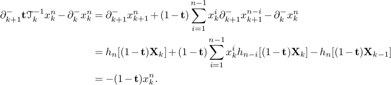 $$ \begin{align*} \partial_{k+1}^- \textbf{t} \mathscr{T}_k^{-1}x_k^{n}- \partial_k^-x_k^n &= \partial_{k+1}^- x_{k+1}^n+(1-\textbf{t})\sum_{i=1}^{n-1}x_k^i \partial_{k+1}^- x_{k+1}^{n-i} - \partial_k^-x_k^n\\ &= h_n[(1-\textbf{t})\mathbf{X}_k]+(1-\textbf{t})\sum_{i=1}^{n-1}x_k^i h_{n-i}[(1-\textbf{t})\mathbf{X}_k] - h_n[(1-\textbf{t})\mathbf{X}_{k-1}]\\ &=-(1-\textbf{t})x_k^n. \end{align*} $$
This proves our claim.
Lemma 7.12. Let $k\geq 1$
,
$k\geq 1$
, $n\geq 0$
,
$n\geq 0$
, $f(x_1,\dots ,x_{k-1})\in \mathscr {P}_{k-1}^{+}$
, and
$f(x_1,\dots ,x_{k-1})\in \mathscr {P}_{k-1}^{+}$
, and $G[\mathbf {X}_{k-1}]\in \operatorname {\mathrm {Sym}}[\mathbf {X}_{k-1}]$
. We regard
$G[\mathbf {X}_{k-1}]\in \operatorname {\mathrm {Sym}}[\mathbf {X}_{k-1}]$
. We regard
 $$ \begin{align*} F=f(x_1,\dots,x_{k-1})x_k^n G[\mathbf{X}_{k-1}] \end{align*} $$
as an element of $\mathscr {P}(k)^+$
. Then,
$\mathscr {P}(k)^+$
. Then,
 $$ \begin{align} (\partial^*_{k-1}\partial_k^- - \partial_{k+1}^-\partial^*_k) F =f(x_2,\dots,x_{k})G[\mathbf{X}_{k}+\textbf{q} x_1](h_n[(1-\textbf{t} )(\mathbf{X}_k+\textbf{q} x_1)]-h_n[(1-\textbf{t} )\mathbf{X}_k]). \end{align} $$
Proof. Straightforward from equation (7.6) and the definition of $\partial ^*$
,
$\partial ^*$
, $\partial ^-$
.
$\partial ^-$
.
7.8
We are now ready to describe the $\mathbb {A}_{\textbf {t},\textbf {q}}$
-module structure on
$\mathbb {A}_{\textbf {t},\textbf {q}}$
-module structure on $\mathscr {P}_{\bullet }$
.
$\mathscr {P}_{\bullet }$
.
Theorem 7.13. The map that sends $T_i$
,
$T_i$
, $d_+$
,
$d_+$
, $d_+^{*}$
and
$d_+^{*}$
and $d^-$
to
$d^-$
to $\mathscr {T}_i$
,
$\mathscr {T}_i$
, $\partial $
,
$\partial $
, $\partial ^*$
and
$\partial ^*$
and $\partial ^-$
, respectively, defines a
$\partial ^-$
, respectively, defines a $\mathbb {A}_{\textbf {t},\textbf {q}}$
-module structure on
$\mathbb {A}_{\textbf {t},\textbf {q}}$
-module structure on $\mathscr {P}_{\bullet }$
. Under this action, the operators
$\mathscr {P}_{\bullet }$
. Under this action, the operators $y_i$
,
$y_i$
, $z_i$
act as
$z_i$
act as $\mathscr {X}_i$
,
$\mathscr {X}_i$
, $\mathscr {Y}_i$
.
$\mathscr {Y}_i$
.
It is important to note that, while the operators corresponding to arrows connecting different nodes are local (i.e., dependent on k), the operators $\mathscr {T}_i$
,
$\mathscr {T}_i$
, $\mathscr {X}_i$
,
$\mathscr {X}_i$
, $\mathscr {Y}_i$
that correspond to loops are global (i.e., independent of k as they are restrictions of operators on
$\mathscr {Y}_i$
that correspond to loops are global (i.e., independent of k as they are restrictions of operators on $\mathscr {P}_{\mathrm {as}}^+$
).
$\mathscr {P}_{\mathrm {as}}^+$
).
Proof. The fact that the operator
 $$ \begin{align*} y_1=\frac{1}{\textbf{t}^{k-1}(\textbf{t}-1)}[d_{+},d_{-}]T_{k-1}\dots T_1 \end{align*} $$
acts on $\mathscr {P}(k)^+$
as
$\mathscr {P}(k)^+$
as $\mathscr {X}_1$
follows from equation (7.9) and the first expression for
$\mathscr {X}_1$
follows from equation (7.9) and the first expression for $\widetilde {\omega }^{-1}_k$
in Remark 3.3. Therefore, for all
$\widetilde {\omega }^{-1}_k$
in Remark 3.3. Therefore, for all $i\geq 1$
, the operator
$i\geq 1$
, the operator $y_i$
acts as
$y_i$
acts as $\mathscr {X}_i$
.
$\mathscr {X}_i$
.
Furthermore, from equations (7.7) and (7.10) and Proposition 6.32, we obtain that
 $$ \begin{align*}z_1T_{1}\cdots T_{k-1}=\frac{\textbf{t}^k}{1-\textbf{t}}[d_{+}^{*},d_{-}] \end{align*} $$
acts on $\mathscr {P}(k)^+$
as
$\mathscr {P}(k)^+$
as $\mathscr {Y}_1 \mathscr {T}_{1}\cdots \mathscr {T}_{k-1}$
. Therefore,
$\mathscr {Y}_1 \mathscr {T}_{1}\cdots \mathscr {T}_{k-1}$
. Therefore, $z_1$
acts on
$z_1$
acts on $\mathscr {P}(k)^+$
as
$\mathscr {P}(k)^+$
as $\mathscr {Y}_1$
and, for all
$\mathscr {Y}_1$
and, for all $i\geq 1$
, the operator
$i\geq 1$
, the operator $z_i$
acts as
$z_i$
acts as $\mathscr {Y}_i$
.
$\mathscr {Y}_i$
.
The verification of many of the relations in Definition 7.3 is virtually identical to the corresponding verification in [Reference Carlsson and Mellit6]. We briefly indicate the main details.
The fact that equations (7.1a) and (7.1b) hold is clear (also part of Theorem 6.34). For the first relation in equation (7.1c), see the proof of the corresponding relation in [Reference Carlsson and Mellit6, Lemma 5.3]; the second set of relations in equation (7.1c) is clear from the definition of the maps involved. For equation (7.1d), recall the expressions for $\widetilde {\omega }^{-1}_k$
in Remark 3.3. With this in mind, the first relation in equation (7.1d) follows from the equality
$\widetilde {\omega }^{-1}_k$
in Remark 3.3. With this in mind, the first relation in equation (7.1d) follows from the equality
 $$ \begin{align} T_1\cdots T_{k+1} T_1\cdots T_k= T_2\cdots T_{k+1} T_1\cdots T_{k+1}, \end{align} $$
which is a consequence of the braid relations. Indeed,
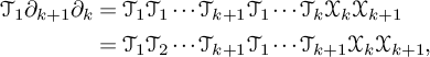 $$ \begin{align*} \mathscr{T}_1\partial_{k+1}\partial_k&=\mathscr{T}_1 \mathscr{T}_1\cdots \mathscr{T}_{k+1} \mathscr{T}_1\cdots \mathscr{T}_k \mathscr{X}_k \mathscr{X}_{k+1}\\ &=\mathscr{T}_1 \mathscr{T}_2\cdots \mathscr{T}_{k+1} \mathscr{T}_1\cdots \mathscr{T}_{k+1} \mathscr{X}_k \mathscr{X}_{k+1}, \end{align*} $$
which on $\mathscr {P}(k)^+$
acts as
$\mathscr {P}(k)^+$
acts as $\mathscr {T}_1 \mathscr {T}_2\cdots \mathscr {T}_{k+1} \mathscr {T}_1\cdots \mathscr {T}_{k} \mathscr {X}_k \mathscr {X}_{k+1}=\partial _{k+1}\partial _k$
. The second set of relations in equation (7.1d) is again a straight consequence of the braid relations.
$\mathscr {T}_1 \mathscr {T}_2\cdots \mathscr {T}_{k+1} \mathscr {T}_1\cdots \mathscr {T}_{k} \mathscr {X}_k \mathscr {X}_{k+1}=\partial _{k+1}\partial _k$
. The second set of relations in equation (7.1d) is again a straight consequence of the braid relations.
For the relations (7.1e), remark that equations (7.9) and (7.1c) and the fact that $\partial ^-_k$
commutes with
$\partial ^-_k$
commutes with $\mathscr {X}_1$
implies the first relation in equaiton (7.1e). The second relation in equaiton (7.1e) follows from equations (7.9) and (7.11).
$\mathscr {X}_1$
implies the first relation in equaiton (7.1e). The second relation in equaiton (7.1e) follows from equations (7.9) and (7.11).
The first relation in equation (7.2a) is a consequence of the fact that an element in the image of $\partial _{k+1}^*\partial _{k}^{*}$
is symmetric in
$\partial _{k+1}^*\partial _{k}^{*}$
is symmetric in $x_1, x_2$
. The second relation in equation (7.2a) is essentially equation (3.3c).
$x_1, x_2$
. The second relation in equation (7.2a) is essentially equation (3.3c).
The first relation in equation (7.2b) can be seen (with the help of equation (7.1c)) to be equivalent to
 $$ \begin{align} \mathscr{Y}_1 \partial_k^-=\partial_k^- \mathscr{Y}_1. \end{align} $$
The commutativity relation is not immediately clear from the definition of the operators involved. We proceed as in the proof of [Reference Carlsson and Mellit6, Proposition 6.3]. More precisely,
 $$ \begin{align*} (\textbf{t}+1)(\partial^- [\partial^*,\partial^-]\mathscr{T}_{k-1}-\textbf{t} [\partial^*,\partial^-] \partial^-)&=(\textbf{t}+1)\partial^-\partial^*\partial^-(\mathscr{T}_{k-1}+\textbf{t}) - \textbf{t} \partial^* (\partial^-)^2(\mathscr{T}_{k-1}+\textbf{t} -\mathscr{T}_{k-1}+1)\\ &\quad +(\partial^-)^2 \partial^* (\mathscr{T}_{k-1}+\textbf{t} -\mathscr{T}_{k-1}+1)\\ &= ((\textbf{t}+1)\partial^-\partial^*\partial^- - \textbf{t} \partial^* (\partial^-)^2 +(\partial^-)^2 \partial^*)(\mathscr{T}_{k-1}+\textbf{t})\\ &= (\partial^- [\partial^*,\partial^-]-\textbf{t} [\partial^*,\partial^-] \partial^-)(\mathscr{T}_{k-1}+\textbf{t}). \end{align*} $$
For the second equality, we used the relations (7.1c) and (7.2a). The image of $\mathscr {T}_{k-1}+\textbf {t}$
lies on the kernel of
$\mathscr {T}_{k-1}+\textbf {t}$
lies on the kernel of $\mathscr {T}_{k-1}-1$
. Therefore, it is enough to check that
$\mathscr {T}_{k-1}-1$
. Therefore, it is enough to check that
 $$ \begin{align*}\partial^- [\partial^*,\partial^-]=\textbf{t} [\partial^*,\partial^-] \partial^- \end{align*} $$
on $\mathscr {P}(k-1)^+\subset \mathscr {P}(k)^+$
. By equaiton (7.8),
$\mathscr {P}(k-1)^+\subset \mathscr {P}(k)^+$
. By equaiton (7.8), $\partial ^-$
acts as an identity on
$\partial ^-$
acts as an identity on $\mathscr {P}(k-1)^+\subset \mathscr {P}(k)^+$
. After examining the action of both sides of the relation on elements in
$\mathscr {P}(k-1)^+\subset \mathscr {P}(k)^+$
. After examining the action of both sides of the relation on elements in $\mathscr {P}(k-1)^+\subset \mathscr {P}(k)^+$
of the form equation (7.7), we see that it is enough to establish the equality for the action on the elements
$\mathscr {P}(k-1)^+\subset \mathscr {P}(k)^+$
of the form equation (7.7), we see that it is enough to establish the equality for the action on the elements $x_{k-1}^n x_k^m+ x_{k-1}^mx_k^n$
,
$x_{k-1}^n x_k^m+ x_{k-1}^mx_k^n$
, $n,m\geq 0$
. The rest of the argument in [Reference Carlsson and Mellit6, Proposition 6.3] applies to conclude the verification of the first relation in equation (7.2b).
$n,m\geq 0$
. The rest of the argument in [Reference Carlsson and Mellit6, Proposition 6.3] applies to conclude the verification of the first relation in equation (7.2b).
For the second relation in equation (7.2b), we proceed as follows. By examining the action of both sides of the relation on elements of the form equation (7.7), we see that it is enough to establish the equality for the action on the elements $x_k^n$
,
$x_k^n$
, $n\geq 0$
. By direct computation,
$n\geq 0$
. By direct computation,
 $$ \begin{align*}[\partial^*,\partial^-]\partial^* x_k^n=h_n[(1-\textbf{t})\mathbf{X}_{k+1}+(1-\textbf{t})\textbf{q} x_1]-h_n[(1-\textbf{t})\mathbf{X}_{k+1}] \end{align*} $$
and
 $$ \begin{align*}\mathscr{T}_1\partial^*[\partial^*,\partial^-]x_k^n=h_n[(1-\textbf{t})\mathbf{X}_{k+1}+(1-\textbf{t})\textbf{q} x_1+(1-\textbf{t})\textbf{q} x_2]-\mathscr{T}_1 h_n[(1-\textbf{t})\mathbf{X}_{k+1}+(1-\textbf{t})\textbf{q} x_1] \end{align*} $$
from which the claimed equality can be readily verified.
The second relation in equation (7.2c) is precisely equation (3.3d). For the first relation in equation (7.2c), it is enough to verify the case $i=1$
, that is,
$i=1$
, that is,
 $$ \begin{align*}\widetilde{\omega}^{-1}_{k+1} \mathscr{Y}_1=\mathscr{Y}_2 \widetilde{\omega}^{-1}_{k+1}. \end{align*} $$
Using the first expression for $\widetilde {\omega }^{-1}_{k+1}$
in Remark 3.3, this reduces to equation (4.1e).
$\widetilde {\omega }^{-1}_{k+1}$
in Remark 3.3, this reduces to equation (4.1e).
The relation (7.2d) is proved as follows
 $$ \begin{align*} \textbf{q} \textbf{t}^{k+1} \mathscr{X}_1 \omega^{-1}_{k+1}&= \textbf{t}^{k+1} \omega^{-1}_{k+1} \mathscr{X}_{k+1}\\ &= \textbf{t}^{k+1} \varpi_{k+1} \mathscr{X}_{k+1}\\ &= \mathscr{Y}_1 \mathscr{T}_1\cdots \mathscr{T}_k \mathscr{X}_{k+1}\\ &= \mathscr{Y}_1 \widetilde{\omega}^{-1}_{k+1}. \end{align*} $$
Therefore,
 $$ \begin{align*}\mathscr{Y}_1 \partial_k=-\textbf{q} \textbf{t}^{k+1} \mathscr{X}_1 \partial^*_{k+1}, \end{align*} $$
as desired.
7.9
We conclude with the comparison of the representations of $\mathbb {A}_{\textbf {t},\textbf {q}}$
in Theorem 7.7 and Theorem 7.13. Let us first define
$\mathbb {A}_{\textbf {t},\textbf {q}}$
in Theorem 7.7 and Theorem 7.13. Let us first define
 $$ \begin{align*} \Phi_{\bullet}=(\Phi_k)_{k \geq 0}: \mathscr{P}_{\bullet} \to V_{\bullet} \end{align*} $$
as follows:
 $$ \begin{align*} \Phi_k:\mathscr{P}(k)^+\cong \mathscr{P}_k^+\otimes \operatorname{\mathrm{Sym}}[\mathbf{X}_k] \to V_k;\quad x_i\mapsto y_i,\quad 1\leq i\leq k;\quad \mathbf{X}_k\mapsto \frac{\mathbf{X}}{\textbf{t}-1}. \end{align*} $$
We note that each $\Phi _k$
is an
$\Phi _k$
is an $\mathbb Q(\textbf {t},\textbf {q})$
-algebra isomorphism.
$\mathbb Q(\textbf {t},\textbf {q})$
-algebra isomorphism.
Theorem 7.14. $\Phi _{\bullet }$
is an isomorphism of
$\Phi _{\bullet }$
is an isomorphism of $\mathbb {A}_{\textbf {t},\textbf {q}}$
-representations.
$\mathbb {A}_{\textbf {t},\textbf {q}}$
-representations.
Proof. We clearly have $\Phi _k T_i=T_i \Phi _k$
for all
$\Phi _k T_i=T_i \Phi _k$
for all $1\leq i\leq k-1$
. We will check that the action of
$1\leq i\leq k-1$
. We will check that the action of $d_+$
satisfies the following equality:
$d_+$
satisfies the following equality:
 $$ \begin{align*} d_{+,k}\Phi_k=\Phi_{k+1}d_{+,k}. \end{align*} $$
Therefore, we only need to prove the correspondence for $d_{+}, d_{+}^{*}, d_{-}$
.
$d_{+}, d_{+}^{*}, d_{-}$
.
Let $F=x_1^{t_1}\ldots x_k^{t_k} f[\mathbf {X}_k] \in \mathscr {P}(k)^+$
. We have,
$F=x_1^{t_1}\ldots x_k^{t_k} f[\mathbf {X}_k] \in \mathscr {P}(k)^+$
. We have,
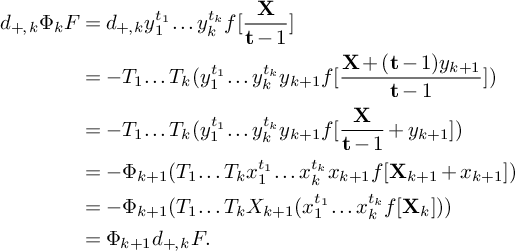 $$ \begin{align*} d_{+,k}\Phi_k F &= d_{+,k}y_1^{t_1}\ldots y_k^{t_k} f[\frac{\mathbf{X}}{\textbf{t}-1}]\\ &=-T_1\ldots T_{k}(y_1^{t_1}\ldots y_k^{t_k}y_{k+1}f[\frac{\mathbf{X}+(\textbf{t}-1)y_{k+1}}{\textbf{t}-1}])\\ &=-T_1\ldots T_{k}(y_1^{t_1}\ldots y_k^{t_k}y_{k+1}f[\frac{\mathbf{X}}{\textbf{t}-1}+y_{k+1}])\\ &=-\Phi_{k+1}(T_1\ldots T_{k}x_1^{t_1}\ldots x_k^{t_k}x_{k+1}f[\mathbf{\mathbf{X}}_{k+1}+x_{k+1}])\\ &=-\Phi_{k+1}(T_1\ldots T_{k}X_{k+1}(x_1^{t_1}\ldots x_k^{t_k}f[\mathbf{\mathbf{X}}_{k}]))\\ &=\Phi_{k+1} d_{+,k} F. \end{align*} $$
Similar computations show that $d^*_{+,k}\Phi _k=\Phi _{k+1}d^*_{+,k}$
and
$d^*_{+,k}\Phi _k=\Phi _{k+1}d^*_{+,k}$
and $d_{-,k}\Phi _k=\Phi _{k-1}d_{-,k}$
.
$d_{-,k}\Phi _k=\Phi _{k-1}d_{-,k}$
.
The following examples illustrate how the actions of $\mathscr {Y}_1$
and
$\mathscr {Y}_1$
and $z_1$
correspond through the isomorphism
$z_1$
correspond through the isomorphism $\Phi _{\bullet }$
.
$\Phi _{\bullet }$
.
Example 7.15. By definition, $\Phi _k(x_2^2)=y_2^2$
for any
$\Phi _k(x_2^2)=y_2^2$
for any $k\geq 2$
. From Example 6.26 and Example 7.9, we have
$k\geq 2$
. From Example 6.26 and Example 7.9, we have
 $$ \begin{align*} \mathscr{Y}_1 \cdot x_2^2&=\textbf{q}^2 \textbf{t}(\textbf{t}-1)x_1^2+\textbf{q}\textbf{t}(\textbf{t}-1)x_1 x_2-\textbf{q}\textbf{t}(\textbf{t}-1)^2 x_1 e_1[\mathbf{X}_2],\\ z_1\cdot y_2^2 &=\textbf{q}^2 \textbf{t}(\textbf{t}-1)y_1^2+\textbf{q}\textbf{t}(\textbf{t}-1)y_1 y_2-\textbf{q}\textbf{t}(\textbf{t}-1)^2 (y_1y_3+\cdots+y_1y_k)-\textbf{q}\textbf{t}(\textbf{t}-1)y_1 e_1[\mathbf{X}]. \end{align*} $$
Now, from the definition of $\Phi _k$
,
$\Phi _k$
, $k\geq 2$
, we can see that
$k\geq 2$
, we can see that
 $$ \begin{align*}\Phi_k(\mathscr{Y}_1 \cdot x_2^2)=z_1\cdot y_2^2. \end{align*} $$
It is important to remark that, while the action of $\mathscr {Y}_1$
on
$\mathscr {Y}_1$
on $x_2^2\in \mathscr {P}(k)^+$
is independent of k, the action of
$x_2^2\in \mathscr {P}(k)^+$
is independent of k, the action of $z_1$
on
$z_1$
on $y_2^2\in V_k$
depends on k.
$y_2^2\in V_k$
depends on k.
Example 7.16. By definition, $\Phi _1(p_2[\mathbf {X}_1])=p_2[\mathbf {X}]/(\textbf {t}^2-1)$
. From Example 6.26 and Example 7.10 for
$\Phi _1(p_2[\mathbf {X}_1])=p_2[\mathbf {X}]/(\textbf {t}^2-1)$
. From Example 6.26 and Example 7.10 for $k=1$
, we have
$k=1$
, we have
 $$ \begin{align*} \mathscr{Y}_1 \cdot p_2[\mathbf{X}_1]&=-\textbf{q}^2 \textbf{t} x_1^2+\textbf{q}\textbf{t}(\textbf{t}-1)x_1 e_1[\mathbf{X}_1],\\ z_1 \cdot p_2[\mathbf{X}]/(\textbf{t}^2-1)&=-\textbf{q}^2 \textbf{t} y_1^2+\textbf{q}\textbf{t} y_1 e_1[\mathbf{X}]. \end{align*} $$
Again, we can see that
 $$ \begin{align*}\Phi_1(\mathscr{Y}_1 \cdot p_2[\mathbf{X}_1])=z_1\cdot p_2[\mathbf{X}]/(\textbf{t}^2-1). \end{align*} $$
For $k=2$
, we have
$k=2$
, we have $\Phi _2(p_2[\mathbf {X}_1])=y_2^2+p_2[\mathbf {X}]/(\textbf {t}^2-1)$
, and from Examples 7.9 and 7.10, we have
$\Phi _2(p_2[\mathbf {X}_1])=y_2^2+p_2[\mathbf {X}]/(\textbf {t}^2-1)$
, and from Examples 7.9 and 7.10, we have
 $$ \begin{align*} \mathscr{Y}_1 \cdot p_2[\mathbf{X}_1]&=-\textbf{q}^2 \textbf{t} x_1^2+\textbf{q}\textbf{t}(\textbf{t}-1)x_1 e_1[\mathbf{X}_1],\\ z_1 \cdot (y_2^2+p_2[\mathbf{X}]/(\textbf{t}^2-1))&=(\textbf{q}^2 \textbf{t}(\textbf{t}-1)y_1^2+\textbf{q}\textbf{t}(\textbf{t}-1)y_1 y_2-\textbf{q}\textbf{t}(\textbf{t}-1)y_1 e_1[\mathbf{X}])\\ &\quad +(-\textbf{q}^2 \textbf{t}^2y_1^2 + \textbf{q}\textbf{t}^2y_1 e_1[\mathbf{X}]) \end{align*} $$
From the definition of $\Phi _2$
, we can see that
$\Phi _2$
, we can see that
 $$ \begin{align*}\Phi_2(\mathscr{Y}_1 \cdot p_2[\mathbf{X}_1])=z_1\cdot (y_2^2+p_2[\mathbf{X}]/(\textbf{t}^2-1)). \end{align*} $$
Again, the action of $\mathscr {Y}_1$
on
$\mathscr {Y}_1$
on $p_2[\mathbf {X}_1]\in \mathscr {P}(k)^+$
is independent of k, while the action of
$p_2[\mathbf {X}_1]\in \mathscr {P}(k)^+$
is independent of k, while the action of $z_1$
on
$z_1$
on $y_2^2+p_2{\mathbf {X}}/(\textbf {t}^2-1)\in V_k$
depends on k.
$y_2^2+p_2{\mathbf {X}}/(\textbf {t}^2-1)\in V_k$
depends on k.
We emphasize that above result is different from the comments in [Reference Carlsson and Mellit6, pg. 694] that suggest a possible algebra isomorphism between $e_k\mathbb {A}_{\textbf {t},\textbf {q}} e_k$
(the subalgebra of
$e_k\mathbb {A}_{\textbf {t},\textbf {q}} e_k$
(the subalgebra of $\mathbb {A}_{\textbf {t},\textbf {q}}$
generated by loops based at node k) and a ‘partially symmetrized’ version of the stable limit spherical DAHA, still to be defined for
$\mathbb {A}_{\textbf {t},\textbf {q}}$
generated by loops based at node k) and a ‘partially symmetrized’ version of the stable limit spherical DAHA, still to be defined for $k>0$
. In particular,
$k>0$
. In particular, $\mathscr {H}^+$
does not contain a copy of the stable limit spherical DAHA which, according to the expectation in [Reference Carlsson and Mellit6], would be isomorphic to
$\mathscr {H}^+$
does not contain a copy of the stable limit spherical DAHA which, according to the expectation in [Reference Carlsson and Mellit6], would be isomorphic to $e_0\mathbb {A}_{\textbf {t},\textbf {q}} e_0$
.
$e_0\mathbb {A}_{\textbf {t},\textbf {q}} e_0$
.
Acknowledgements
The work of BI was partially supported by the Simons Foundation grant 420882.
Competing Interests
None.


 Open access