


1. Introduction
Gardner Murphy, an influential social and personality psychologist, defined learning as something that covers every modification in the behavior to meet the requirements of the environment (Proshansky & Murphy, Reference Proshansky and Murphy1942). Humans and animals rely heavily on the process of trial-and-error to acquire new skills. Experiences like learning how to walk, riding a bicycle, teaching a dog new tricks are all motivated by performing actions that garner positive rewards (e.g., moving forward, not falling, happiness, and getting treats). Such interactions become a significant source of knowledge about new things and uncertain environments. Reinforcement Learning (RL) is a paradigm of Machine Learning (ML) that teaches an agent, a learner, to make sequential decisions in a potentially complex, uncertain environment with the fundamental goal to maximize its overall reward.
Exponential growth in computational power, custom-developed Application Specific Integrated Circuit (ASIC) (Barr, Reference Barr2007), Tensor Processing Units (TPUs)Footnote 1 combined with the availability of enormous training datasets has accelerated training workloads and led to an unprecedented surge of interest in the topic of Deep Reinforcement Learning (DRL), especially in domains like telecommunications (Nikou et al., to appear; Luong et al., Reference Luong2019; Yajnanarayana et al., Reference Yajnanarayana, Ryden and Hevizi2020), networking (Kavalerov et al., Reference Kavalerov, Likhacheva and Shilova2017; Luong et al., Reference Luong2019), game-playing agents (Bellemare et al., Reference Bellemare, Naddaf, Veness and Bowling2013; Mnih et al., Reference Mnih and Kavukcuoglu2015; Silver et al., Reference Silver and Huang2016; Brockman et al., Reference Brockman, Cheung, Pettersson, Schneider, Schulman, Tang and Zaremba2016), robotic manipulations (Abbeel et al., Reference Abbeel, Coates, Quigley and Ng2006; Kalashnikov et al., Reference Kalashnikov2018), and recommender systems (Zheng et al., Reference Zheng, Zhang, Zheng, Xiang, Yuan, Xie and Li2018; Munemasa et al., Reference Munemasa2018).
1.1. Problem
Deep Q-Network (DQN) (Mnih et al., Reference Mnih and Kavukcuoglu2015) uses Neural Networks (NNs) as function approximators to estimate the Q-function, it does so by making enhancements to the original Q-learning algorithm by employing an experience replay buffer and a separate target network that is updated less frequently. Actor-critic algorithms like Asynchronous Advantage Actor Critic (A3C) utilize Monte Carlo samples to estimate the gradients and then learn the parameters of the policy using gradient descent. Revised variants of these algorithms have been published over the past few years, which have improved performance on several complex problems and industry standard benchmarks (Lillicrap et al., Reference Lillicrap2015; van Hasselt et al., Reference van Hasselt, Guez and Silver2016; Wang et al., Reference Wang, Schaul, Hessel, Hasselt, Lanctot and Freitas2016; Silver et al., Reference Silver and Hubert2017). However, all of these approaches entail expensive computations, such as calculating gradients and backpropagation, to train neural networks. Training such models take several hours, even multiple days (Mnih et al., Reference Mnih, Badia, Balcan and Weinberger2016; Mania et al., Reference Mania, Guy and Recht2018), to obtain satisfactory results, mainly when applied to problems that have a very large state space. Some other drawbacks of these algorithms include the sensitivity to the different hyperparameters, poor sample efficiency (Yu, Reference Yu2018), and limited parallelizability.
Recent publications, notably from OpenAI (Salimans et al., Reference Salimans2017) and UberAI (Conti et al., Reference Conti, Madhavan, Such, Lehman, Stanley and Clune2018), exhibited the use of Evolutionary Computation (EC) to train deep neural networks for RL problems. The combined use of EC and RL offers several advantages. These gradient-free methods are more robust to the issues of dense and sparse rewards and are also more tolerant to longer time horizons. The inherent design of such algorithms makes them well suited for distributed training which has shown significant speedup of overall training time (Salimans et al., Reference Salimans2017; Conti et al., Reference Conti, Madhavan, Such, Lehman, Stanley and Clune2018).
1.2. Research question
The research questions we are looking to address in the current work are:
-
1. How effective are gradient-free evolutionary-driven methods, such as variants of Genetic Algorithms (GAs), in training deep neural networks for RL problems with a large state space? How do they compare to gradient-based algorithms in terms of performance and training time?
-
2. To what extent can evolution-based RL algorithms be scaled? Are the gains worth the extra number of workers?
-
3. How effective are evolution-based methods when applied to RL problems in different domains like the optimization of Remote Electrical Tilt (RET) in telecommunications?
1.3. Contribution
In this work, a novel species-based GA that trains a deep neural network for RL specific problems is proposed. The algorithm which is model-free, gradient-free only utilizes simple genetic operators like mutation, selection, recombination, and crossover for training. A memory efficient encoding of the neural network is presented which simplifies the application of genetic operators and also reduces bandwidth requirement making this approach highly scalable.
1.4. Purpose
The key benefits of using EC-based techniques for training neural networks are the simplicity of implementation, a faster rate of convergence due to distributed training, and the reduced number of hyperparameters. Population-based methods, if implemented efficiently, are massively scalable due to their inherent design and can achieve a significant parallel speedup. The reduced training time makes them well suited for RL problems that require frequent retraining and for those that require multiple policies. Since the method is gradient-free, it does not suffer from known issues of exploding, vanishing gradients and is particularly well suited for non-differentiable domains (Cho et al., Reference Cho2014; Xu et al., Reference Xu2016; Liu et al., Reference Liu2018). Some additional advantages of these black-box optimization techniques include: the improved exploration (Conti et al., Reference Conti, Madhavan, Such, Lehman, Stanley and Clune2018) due to their stochastic nature and the invariance to the scale of rewards (sparse/dense) which is something that has to be addressed explicitly in current state-of-the-art methods.
Our work can also be combined with existing Markov Decision Process (MDP)-based methods to develop a hybrid approach. The use of EC-based training for neural networks can also be extended to supervised learning tasks. Lastly, neuroevolution and its application to RL is thought to be one step toward artificial general intelligence, which is a topic of significant interest to researchers all over the world.
1.5. Ethics and sustainability
A recent research study (Strubell et al., Reference Strubell, Ganesh and Mccallum2019) highlighted that training a deep learning model can generate over 600 000 pounds of $CO_2$
emissions. In comparison, an average Swedish person generates around 22 000 poundsFootnote 2 of
$CO_2$
emissions. In comparison, an average Swedish person generates around 22 000 poundsFootnote 2 of $CO_2$
emissions(as of 2020) per year. These numbers, when compared, are pretty concerning. Deep learning models for RL rely on specialized hardware like Graphics Processing Units (GPUs) and TPUs which are not only expensive but also consume significant amount of power (Jouppi et al., Reference Jouppi2017). The long training times (Mnih et al., Reference Mnih and Kavukcuoglu2015; Mnih et al., Reference Mnih, Badia, Balcan and Weinberger2016; van Hasselt et al., Reference van Hasselt, Guez and Silver2016) makes the matter much worse. GPUs require an efficient cooling system and maintenance, or else it can thermal throttle, which adversely effects its efficiency and life.
$CO_2$
emissions(as of 2020) per year. These numbers, when compared, are pretty concerning. Deep learning models for RL rely on specialized hardware like Graphics Processing Units (GPUs) and TPUs which are not only expensive but also consume significant amount of power (Jouppi et al., Reference Jouppi2017). The long training times (Mnih et al., Reference Mnih and Kavukcuoglu2015; Mnih et al., Reference Mnih, Badia, Balcan and Weinberger2016; van Hasselt et al., Reference van Hasselt, Guez and Silver2016) makes the matter much worse. GPUs require an efficient cooling system and maintenance, or else it can thermal throttle, which adversely effects its efficiency and life.
The algorithm proposed in this work does not compute gradients and does not perform back-propagation, both of which are computationally expensive tasks. Lack of gradients means that low precision older hardware and only Central Processing Units (CPUs)s can be used as workers during training. Although a parallel implementation utilizes multiple workers, this is well compensated by the significant reduction of training time as evidenced in the experiments. This approach can also benefit researchers and organizations that do not have access to specialized hardware and cloud-based instances.
1.6. Delimitations
The work aims not to break the records on the Atari 2600 benchmarks but to serve as a proof of concept and explore the potential of a novel approach.
The experiments rely on two open-source libraries, gymFootnote 3 for the environments used for benchmarking and rllibFootnote 4 for the reference implementation of DQN, A3C, and ES. The exact replication of the results is dependant on the specific versions of these libraries.
Due to limited resources and time constraints, the same hyperparameters are used for all Atari 2600 games and a single run is performed. Training is limited to a maximum of 25 million training frames on 16 games—some chosen at random while others were chosen from the publication Deep Neuroevolution (Conti et al., Reference Conti, Madhavan, Such, Lehman, Stanley and Clune2018).
2. Background
2.1. Reinforcement learning
RL is inherently different from supervised tasks where labeled samples containing both inputs and targets are available for training. For control problems that involve interaction with an entity or an environment, obtaining samples that are both representative and correct for all situations is often unrealistic. RL tackles this problem by allowing a goal-seeking agent to interact with an uncertain environment. This agent is responsible for maintaining a balance between exploration and exploitation to build a rich experience which it uses as a memory to make better decisions progressively.
A RL system can be characterized by the following elements:
-
• Policy: The agent interacts with an environment at discrete time steps $t=0,1,2,3, \ldots$
. The policy is a rule that guides the agent on what actions (
$a_{t}$
) to take. It does so by creating a mapping from states (
$s_{t}$
), a perceived representation of the environment, and possible actions. Policies can either be deterministic, usually denoted by
$\mu$
,
$a_{t}=\mu(s_{t})$
, or they can be stochastic, which are usually denoted by
$\pi$
,
$a_{t} \sim \pi\!\left(\cdot \mid s_{t}\right)$
, representing the probability of taking an action at a particular state.
$t=0,1,2,3, \ldots$
. The policy is a rule that guides the agent on what actions (
$a_{t}$
) to take. It does so by creating a mapping from states (
$s_{t}$
), a perceived representation of the environment, and possible actions. Policies can either be deterministic, usually denoted by
$\mu$
,
$a_{t}=\mu(s_{t})$
, or they can be stochastic, which are usually denoted by
$\pi$
,
$a_{t} \sim \pi\!\left(\cdot \mid s_{t}\right)$
, representing the probability of taking an action at a particular state. -
• Rewards: are responses from the environment. They represent the immediate and intrinsic appeal of taking a particular action in a specific state.
-
• Value function: is the maximal expected reward that can be accumulated over the future, starting from a particular state. This takes into account the long-time desirability of the state, which makes it different from rewards that provide an immediate response.
-
• Model: It represents the system dynamics of the environment. The presence of a model can help the agent make better predictions and learn faster.


The agent interacts with the environment in a sequence of time steps. At each time step, it observes a representation of the environment, that is, its state $s_t \in \mathcal{S}$
, and then decides to take action
$s_t \in \mathcal{S}$
, and then decides to take action $a_t \in \mathcal{A}$
by following a policy. As a consequence of its action, the agent receives an immediate reward from the environment,
$a_t \in \mathcal{A}$
by following a policy. As a consequence of its action, the agent receives an immediate reward from the environment, $r_t$
, and transitions to the next state,
$r_t$
, and transitions to the next state, $s_{t+1}$
. The agent’s objective is to learn a policy to maximize its cumulative reward over a time horizon. This fixed horizon is also known as a trajectory (
$s_{t+1}$
. The agent’s objective is to learn a policy to maximize its cumulative reward over a time horizon. This fixed horizon is also known as a trajectory ( $\tau$
) or an episode.
$\tau$
) or an episode.
 \begin{equation} \tau = s_{0}, a_{0}, r_{1}, s_{1}, a_{1}, r_{2}, s_{2}, a_{2}, r_{3}, \ldots\end{equation}
This interaction can be seen in Figure 1.

Figure 1. Interaction of an agent with the environment at a time step t. Image credits (Sutton & Barto, Reference Sutton and Barto2018)
2.1.1. Markov decision process
The elements of an Reinforcement Learning (RL) problem, as described in Section 2.1 can be formalized using the Markov Decision Process (MDP) framework (Puterman, Reference Puterman1994; Boutilier et al., Reference Boutilier, Dean and Hanks1999). Markov Decision Process (MDP) can efficiently model the interactions between the environment and the agent by defining a tuple $\langle \mathcal{S}, \mathcal{A}, \mathcal{P}, \mathcal{R}\rangle$
, where:
$\langle \mathcal{S}, \mathcal{A}, \mathcal{P}, \mathcal{R}\rangle$
, where:
-
•
$\mathcal{S}$
represents the finite set of states,
$s_{t} \in \mathcal{S}$
with dimensionality N, that is,
$|\mathcal{S}|=N$
. Recall, a state is a distinctive characteristic of the environment or the problem being modeled. -
•
$\mathcal{A}$
represents the finite set of actions,
$a_{t} \in \mathcal{A}$
with dimensionality K, that is,
$|\mathcal{A}|=K$
. Each action
$a_t$
is used as a control to interact with the environment at time t. A set of available actions at a particular state s is denoted by A(s), where
$A(s) \subseteq \mathcal{A}$
. -
•
$ \mathcal{P}\,{:}\, \mathcal{S} \times \mathcal{A} \times \mathcal{S} \rightarrow[0,1]$
is the stochastic transition function, where
$p\left(s^{\prime} \mid s, a\right)$
, also denoted as
$p_{s, s^{\prime}}^a$
is the probability of transitioning to state
$s^{\prime}$
by taking action a at state s. These transition probabilities can also be stationary, that is, they are independent of time t.


 \begin{equation} p\left(s^{\prime} \mid s, a\right)=p_{s, s^{\prime}}^a=\mathbb{P}\!\left\{s_{t+1}=s^{\prime} \mid s_{t}=s, a_{t}=a\right\}. \end{equation}
For this transition function to represent a proper probability distribution the following properties must hold:
 \begin{equation} p\!\left(s^{\prime} \mid s, a\right) \geq 0 \text { and } p\!\left(s^{\prime} \mid s, a\right) \leq 1 \end{equation}
 \begin{equation} \sum_{s^{\prime} \in S} p\!\left(s^{\prime} \mid s, a\right)=1 \end{equation}
Since MDPs are controlled Markov chains (Markov, Reference Markov1906; Markov, Reference Markov2006), the distribution of state at time $t+1$
is independent of the past given the state at time t and the action performed by the agent.
$t+1$
is independent of the past given the state at time t and the action performed by the agent.
 \begin{align} \mathbb{P}\!\left[s_{t+1}=s^{\prime} \mid s_{t}, a_{t}, s_{t-1}, a_{t-1}, \ldots\right]=\mathbb{P}\!\left[s_{t+1}=s \mid s_{t}, a_{t}=a\right] \\[-20pt] \nonumber \end{align}
-
•
$\mathcal{R}\,{:}\, \mathcal{S} \times \mathcal{A} \times \mathcal{S} \rightarrow \mathbb{R}$
is the state reward function. It is a scalar value,
$r\!\left(s, a, s^{\prime}\right)$
, also denoted as
$r_{s, s^{\prime}}^a$
, which is awarded to the agent for transitioning from state s to
$s^\prime$
by performing an action a. (6)Alternatively, rewards can also be defined as
\begin{equation} r\!\left(s, a, s^{\prime}\right)=\mathcal{R}_{s, s^{\prime}}^a=\mathbb{E}\!\left\{R_{t+1}\mid s_{t}=s, a_{t}=a,s_{t+1}=s^{\prime}\right\}. \end{equation}
$R\,{:}\, S \times A \rightarrow \mathbb{R}$
where a reward is awarded for taking an action in a state. (7)
\begin{equation} r\!\left(s, a\right)=t_{s, a}=\mathbb{E}\!\left\{R_{t+1}\mid s_{t}=s, a_{t}=a\right\}. \end{equation}


2.1.2. Policies and optimality criteria
In the previous section, we have defined a mathematical formalism for RL problems using an MDP. To formally determine the expected return, $G_t$
that is, objective that the policy seeks to optimize, two classes of MDPs are discussed:
$G_t$
that is, objective that the policy seeks to optimize, two classes of MDPs are discussed:
-
• Finite Horizon : Given a fixed time horizon of T, the objective is to find a sequential decision policy
$\pi$
, that maximizes the expected return until the end of the time horizon. If we represent the sequence of rewards received after time t, by
$r_{t+1}, r_{t+2}, r_{t+3}, \ldots$
, then the cumulative reward is simply: (8)
\begin{equation} G_{t} \doteq r_{t+1}+r_{t+2}+r_{t+3}+\cdots+r_{T} \end{equation}
-
• Infinite Horizon—Discounted rewards : Given an endless time horizon
$T=\infty$
, the objective is to find a sequential decision policy,
$\pi$
that maximizes the expected discounted return. (9)where
\begin{equation} G_{t} \doteq r_{t+1}+\lambda r_{t+2}+\lambda^{2} r_{t+3}+\cdots=\sum_{l=0}^{\infty} \lambda^{l} r_{t+l+1} \end{equation}
$\lambda$
is a parameter,
$0 \leq \lambda<1$
, which discounts the future rewards, the rewards received after l time steps are worth
$\lambda^{l-1}$
times their original value. The discounting of rewards also ensures that the expected return converges. The following recursive relation between the rewards of successive time steps is the key result used in several RL algorithms.(10)
\begin{align} G_{t} & \doteq r_{t+1}+\lambda r_{t+2}+\lambda^{2} r_{t+3}+\lambda^{3} r_{t+4}+\cdots \nonumber \\[3pt] & =r_{t+1}+\lambda\!\left(r_{t+2}+\lambda r_{t+3}+\lambda^{2} r_{t+4}+\cdots\right) \nonumber\\[3pt] & =r_{t+1}+\lambda G_{t+1} \\[-30pt] \nonumber \end{align}


2.1.3. Value functions and Bellman equation
A stochastic policy $\pi$
, is a mapping from a state
$\pi$
, is a mapping from a state $s\in \mathcal{S}$
to action
$s\in \mathcal{S}$
to action $a\in\mathcal{A}(s)$
. It represents the probability of taking action a in state s,
$a\in\mathcal{A}(s)$
. It represents the probability of taking action a in state s, $\pi(a \mid s)$
. The state-value function, or simply value function, for a state s under a policy
$\pi(a \mid s)$
. The state-value function, or simply value function, for a state s under a policy $\pi$
is denoted as
$\pi$
is denoted as $v_{\pi}(s)$
. It is the expected reward that can be accumulated starting with state s and following the policy
$v_{\pi}(s)$
. It is the expected reward that can be accumulated starting with state s and following the policy $\pi$
thereafter. For an infinite horizon model as described in the previous section, the state-value function can be formalized as:
$\pi$
thereafter. For an infinite horizon model as described in the previous section, the state-value function can be formalized as:
 \begin{equation} v_{\pi}(s) \doteq \mathbb{E}_{\pi}\!\left[G_{t} \mid S_{t}=s\right]=\mathbb{E}_{\pi}\!\left[\sum_{l=0}^{\infty} \lambda^{l} R_{t+l+1} \mid S_{t}=s\right]\end{equation}
Similarly, state-action-value function $Q\,{:}\, S \times A \rightarrow \mathbb{R}$
is defined as the expected reward that can be gathered starting with state s, taking an action a and following the policy
$Q\,{:}\, S \times A \rightarrow \mathbb{R}$
is defined as the expected reward that can be gathered starting with state s, taking an action a and following the policy $\pi$
thereafter.
$\pi$
thereafter.
 \begin{equation} q_{\pi}(s, a) \doteq \mathbb{E}_{\pi}\!\left[G_{t} \mid S_{t}=s, A_{t}=a\right]=\mathbb{E}_{\pi}\!\left[\sum_{l=0}^{\infty} \lambda^{l} R_{t+l+1} \mid S_{t}=s, A_{t}=a\right]\end{equation}
A recursive formulation of Equation (11) which relates the value function of a state ( $v_{\pi}(s)$
) to the value function of its successor states (
$v_{\pi}(s)$
) to the value function of its successor states ( $v_{\pi}(s')$
) is a fundamental result utilized throughout RL. It is known as the Bellman equation (Bellman, Reference Bellman1958):
$v_{\pi}(s')$
) is a fundamental result utilized throughout RL. It is known as the Bellman equation (Bellman, Reference Bellman1958):
 \begin{equation} \begin{aligned} v_{\pi}(s) & \doteq \mathbb{E}_{\pi}\!\left[G_{t} \mid S_{t}=s\right] \\[3pt] & =\mathbb{E}_{\pi}\!\left[r_{t+1}+\lambda G_{t+1} \mid S_{t}=s\right] \\[3pt] & =\sum_{a} \pi(a \mid s) \sum_{s^{\prime}} \sum_{r} p\!\left(s^{\prime}, r \mid s, a\right)\!\left[r+\lambda \mathbb{E}_{\pi}\!\left[G_{t+1} \mid S_{t+1}=s^{\prime}\right]\right] \\[3pt] & =\sum_{a} \pi(a \mid s) \sum_{s^{\prime}, r} p\!\left(s^{\prime}, r \mid s, a\right)\!\left[r+\lambda v_{\pi}\!\left(s^{\prime}\right)\right] \end{aligned}\end{equation}
A policy $\pi$
is considered better than
$\pi$
is considered better than $\pi^{\prime}$
iff
$\pi^{\prime}$
iff $v_{\pi}(s) \geq v_{\pi^{\prime}}(s)$
for all states
$v_{\pi}(s) \geq v_{\pi^{\prime}}(s)$
for all states $s \in \mathcal{S}$
. The policy which is better than all is known as the optimal policy:
$s \in \mathcal{S}$
. The policy which is better than all is known as the optimal policy: $\pi_{*}$
, its value function, denoted by
$\pi_{*}$
, its value function, denoted by $v_{*}$
, can be formulated as:
$v_{*}$
, can be formulated as:
 \begin{equation} \begin{array}{l} \qquad v_{*}(s) \doteq \max _{\pi} v_{\pi}(s), \text { for all } s \in \mathcal{S}. \end{array}\end{equation}
The optimal state-action-value function, denoted by $q_{*}$
, can be formulated as:
$q_{*}$
, can be formulated as:
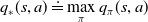 \begin{equation} q_{*}(s, a) \doteq \max _{\pi} q_{\pi}(s, a)\end{equation}
The Bellman optimality equation declares that the value function of a state under the optimal policy is the expected return received from the ‘best (greedy)’ action in that state.
 \begin{equation} \begin{aligned} v_{*}(s) & =\max _{a \in \mathcal{A}(s)} q_{\pi_{*}}(s, a) \\[3pt] & =\max _{a} \mathbb{E}_{\pi_{*}}\!\left[G_{t} \mid S_{t}=s, A_{t}=a\right] \\[3pt] & =\max _{a} \mathbb{E}_{\pi_{*}}\!\left[r_{t+1}+\lambda G_{t+1} \mid S_{t}=s, A_{t}=a\right] \\[3pt] & =\max _{a} \mathbb{E}\!\left[r_{t+1}+\lambda v_{*}\!\left(S_{t+1}\right) \mid S_{t}=s, A_{t}=a\right] \\[3pt] & =\max _{a} \sum_{s^{\prime}, r} p\!\left(s^{\prime}, r \mid s, a\right)\!\left[r+\lambda v_{*}\!\left(s^{\prime}\right)\right]. \end{aligned}\end{equation}
Similarly, the bellman optimality equation for $q_{*}$
, can be formulated as:
$q_{*}$
, can be formulated as:
 \begin{equation} \begin{aligned} q_{*}(s, a) & =\mathbb{E}\!\left[r_{t+1}+\lambda \max _{a^{\prime}} q_{*}\!\left(S_{t+1}, a^{\prime}\right) \mid S_{t}=s, A_{t}=a\right] \\[3pt] & =\sum_{s^{\prime}, r} p\!\left(s^{\prime}, r \mid s, a\right)\!\left[r+\lambda \max _{a^{\prime}} q_{*}\!\left(s^{\prime}, a^{\prime}\right)\right] \end{aligned}\end{equation}
2.2. RL algorithms
Model-based RL algorithms rely on the availability of the transition and reward function. The critical component of such techniques is ‘planning.’ The agent can plan and make predictions about its possible options and use it to improve the policy (Figure 2).
A major challenge of these techniques is the unavailability of the ground truth model, resulting in a bias where the agent performs poorly when tested in the real environment. In this work, we primarily focus on model-free RL.
Model-free methods don’t require a model and primarily rely on ‘learning’ the value functions directly.

Figure 2. Workflow for model-based learning techniques
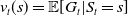
2.2.1. Dynamic programming
When the model for the problem is known, dynamic programming (Bellman, Reference Bellman1954), a mathematical optimization technique, can be utilized to learn the optimal policy. Generalized Policy Iteration (GPI) is such an approach, and it uses an iterative two-step procedure to learn the optimal policy.
-
1. Policy evaluation: The first step evaluates the state-value function
$v_{\pi}$
using the recursive formulation in Equation (13). -
2. Policy improvement: The second step uses the value function to generate an improved policy
$\pi' \geq \pi$
using a greedy approach formulated in Equation (17).


Since the improved policy $\pi'$
is greedy in actions to the current policy, that is,
$\pi'$
is greedy in actions to the current policy, that is, $\pi'(s) = \arg\max_{a \in \mathcal{A}} q_\pi(s, a)$
 \begin{equation} \begin{aligned} q_\pi(s, \pi'(s)) & = q_\pi(s, \arg\max_{a \in \mathcal{A}} q_\pi(s, a)) \\[3pt] & = \max_{a \in \mathcal{A}} q_\pi(s, a) \geq q_\pi(s, \pi(s)) = v_\pi(s) \end{aligned}\end{equation}
this iterative process is guaranteed to converge to the optimal value (Sutton & Barto, Reference Sutton and Barto2018).
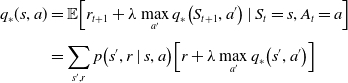
2.2.2. Monte Carlo techniques
Monte Carlo techniques estimate the value functions without the need of system dynamics of the environment making it a model-free method. They rely on complete episodes to approximate the expected return, $G_{t}$
of a state. Recall, the value function,
$G_{t}$
of a state. Recall, the value function, $v_t(s) = \mathbb{E}[ G_t \vert S_t=s]$
. In an episode,
$v_t(s) = \mathbb{E}[ G_t \vert S_t=s]$
. In an episode, $s_{0}, a_{0}, r_{1}, s_{1}, a_{1}, r_{2}, s_{2}, a_{2}, r_{3}, \ldots$
, the occurrence of a state s is known as the visit to s. First-Visit Monte Carlo algorithm estimates the value function as the average of the returns (
$s_{0}, a_{0}, r_{1}, s_{1}, a_{1}, r_{2}, s_{2}, a_{2}, r_{3}, \ldots$
, the occurrence of a state s is known as the visit to s. First-Visit Monte Carlo algorithm estimates the value function as the average of the returns ( $G_t$
) following the first visits to s whereas Every-Visit Monte Carlo algorithm estimates it as the average of the returns following every visit to s.
$G_t$
) following the first visits to s whereas Every-Visit Monte Carlo algorithm estimates it as the average of the returns following every visit to s.
The optimal policy is then evaluated using the same GPI explained previously. The schematic is shown in Figure 3.
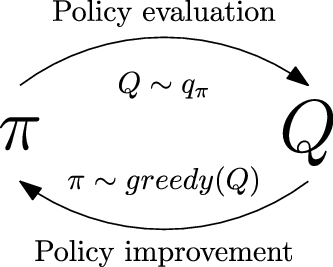
Figure 3. GPI iterative process for optimal policy
2.2.3. Temporal-difference methods
Temporal Difference (TD) methods are model-free. Unlike MC methods, where the agents wait until the end of the episode for the final return to estimate the value functions, TD methods rely on an estimated final return, $r_{t+1} + \lambda v(s_{t+1})$
known as the TD target. The state-value function and state-action-value function are estimated at every step using the below formulation:
$r_{t+1} + \lambda v(s_{t+1})$
known as the TD target. The state-value function and state-action-value function are estimated at every step using the below formulation:
 \begin{equation} \begin{aligned} v(s_t) & \leftarrow v(s_t) + \alpha (r_{t+1} + \lambda v(s_{t+1}) - v(s_t)) \end{aligned}\end{equation}
 \begin{equation} \begin{aligned} q\!\left(s_{t}, a_{t}\right) & \leftarrow q\!\left(s_{t}, a_{t}\right)+\alpha\!\left(r_{t+1}+\lambda q\!\left(S_{t+1}, a_{t+1}\right)-q\!\left(s_{t}, a_{t}\right)\right) \end{aligned}\end{equation}
where $\alpha$
is a hyperparameter called the learning rate, which controls the rate at which the value gets updated at each step. This technique is called bootstrapping because the target value is updated using the current estimate of the return (
$\alpha$
is a hyperparameter called the learning rate, which controls the rate at which the value gets updated at each step. This technique is called bootstrapping because the target value is updated using the current estimate of the return ( $r_{t+1} + \lambda v(s_{t+1})$
) and not the exact return,
$r_{t+1} + \lambda v(s_{t+1})$
) and not the exact return, $G_t$
.
$G_t$
.
2.2.4. Policy gradient
The methods discussed so far estimate the state-value, state-action-value functions respectively to learn what actions to take to maximize the overall return. Policy gradient consists of a family of methods that learn a parameterized policy without computing these value functions. A stochastic policy, parameterized with a set of parameters, $\theta \in \mathbb{R}^{d}$
, can be represented as,
$\theta \in \mathbb{R}^{d}$
, can be represented as, $\pi(a \mid s, \theta)=p\!\left(A_{t}=a \mid S_{t}=s, \boldsymbol{\theta}_{t}=\theta\right)$
, that is, the probability of taking an action at given state with a set of parameters
$\pi(a \mid s, \theta)=p\!\left(A_{t}=a \mid S_{t}=s, \boldsymbol{\theta}_{t}=\theta\right)$
, that is, the probability of taking an action at given state with a set of parameters $\theta$
at time t.
$\theta$
at time t.
The parameters are learned by computing the gradient of an objective function, $J(\theta)$
, a scalar quantity that measures the performance of the policy. The goal of these methods is to maximize the performance by updating the parameters of the policy using stochastic gradient ascent (Bottou, Reference Bottou1998) as
$J(\theta)$
, a scalar quantity that measures the performance of the policy. The goal of these methods is to maximize the performance by updating the parameters of the policy using stochastic gradient ascent (Bottou, Reference Bottou1998) as
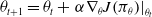 \begin{equation} \theta_{t+1}=\theta_{t}+\left.\alpha \nabla_{\theta} J\!\left(\pi_{\theta}\right)\right|_{\theta_{t}}\end{equation}
where $\nabla_{\theta} J\!\left(\pi_{\theta}\right) \in \mathbb{R}^{d}$
is an estimate whose expectation is equivalent to the gradient of the policy’s performance, known as policy gradient.
$\nabla_{\theta} J\!\left(\pi_{\theta}\right) \in \mathbb{R}^{d}$
is an estimate whose expectation is equivalent to the gradient of the policy’s performance, known as policy gradient.
2.2.5. Actor-critic methods
They consist of algorithms that rely on estimating the parameters of the value functions (state-value or state-action-value function) concurrently with the policy. The two components include:
-
1. Actor: is responsible for the agent’s policy, that is, it is used to pick out which action to perform. The underlying objective is to update the parameters of the policy using Equation (21) guided by the estimates from the critic as the baseline.
-
2. Critic: is responsible for estimating the agent’s value functions. The objective is to update the parameters,
$\phi$
, of the state-value function,
$v(s;\ \phi)$
, or the state-action-value function,
$q(s,a;\ \phi)$
by computing the TD error,
$\delta_t$
as (22)Figure 4 shows the working of an actor-critic method.
\begin{equation} \delta_{t}=r_{t+1}+\lambda v\!\left(s_{t+1}\right)-v(s_{t}) \end{equation}
Figure 4. Architecture for actor-critic methods (Sutton & Barto, Reference Sutton and Barto2018)


2.3. Artificial neural networks
Artificial Neural Networks (ANNs), often referred to as NNs, were first proposed several decades ago (Fitch, Reference Fitch1944). The formulation of these methods is heavily inspired by the human brain, a highly intricate organ that is made up of over 100 billion neurons (Herculano-Houzel, Reference Herculano-Houzel2009). Each neuron is a specialized nerve cell that transmits electrochemical signals to other neurons, gland cells, muscles, etc., which further perform specialized tasks. With such an interconnected network of neurons, our brain is able to carry out quite complex tasks. This mechanism is what ANNs are based on.
2.3.1. Mathematical model
A NN is a computational model that consists of an input layer, hidden layers (any number), and an output layer. Each layer consists of several artificial neurons, the fundamental units of the network, which define a function on the inputs. Any network that uses several hidden layers (usually more than 3) is referred to as a Deep Neural Network (DNN), and the paradigm of ML that deals with DNN is known as Deep Learning (DL) (Goodfellow et al., Reference Goodfellow, Bengio and Courville2016).
In a feed-forward network, the interconnections between the nodes, that is, the neurons, do not form a cycle. Network topologies where the connections between neurons include a directed graph over a temporal sequence are known as Recurrent Neural Networks (RNNs). In this work, we primarily focus on a feed-forward network which is trained by performing a forward pass, also referred as forward propagation and a subsequent backward pass, also known as backpropagation.
Forward Propagation: When training a NN, the forward pass is the calculation phase, sometimes referred to as the evaluation phase. The input signals are forward propagated through all the neurons in each network layer in a sequential manner. The activation of a single neuron is shown in Figure 5, where the input signals $x_1,x_2\ldots x_n$
are first multiplied by a set of weights,
$x_1,x_2\ldots x_n$
are first multiplied by a set of weights, $w_{i,j}$
, and then combined with a bias term,
$w_{i,j}$
, and then combined with a bias term, $b_j$
to obtain a pre-activation signal,
$b_j$
to obtain a pre-activation signal, $z_j$
. The bias is usually utilized to offset the pre-activation signal in case of an all-zero input; at times, this can alternatively be seen as an additional weight that is applied to an input, that is, a constant 1.
$z_j$
. The bias is usually utilized to offset the pre-activation signal in case of an all-zero input; at times, this can alternatively be seen as an additional weight that is applied to an input, that is, a constant 1.

Figure 5. Activation of a single neuron in the neural network
An activation function, $g_j$
is then applied to
$g_j$
is then applied to $z_j$
to obtain the final output signal of the neuron. The process is then repeated across all neurons of each layer one by one until the final output is received. Figure 6 shows the forward propagation in a NN with a single hidden layer of 3 neurons. The final output,
$z_j$
to obtain the final output signal of the neuron. The process is then repeated across all neurons of each layer one by one until the final output is received. Figure 6 shows the forward propagation in a NN with a single hidden layer of 3 neurons. The final output, $x_k$
, is the prediction made by the NN given the input. This completes the forward pass of the network.
$x_k$
, is the prediction made by the NN given the input. This completes the forward pass of the network.
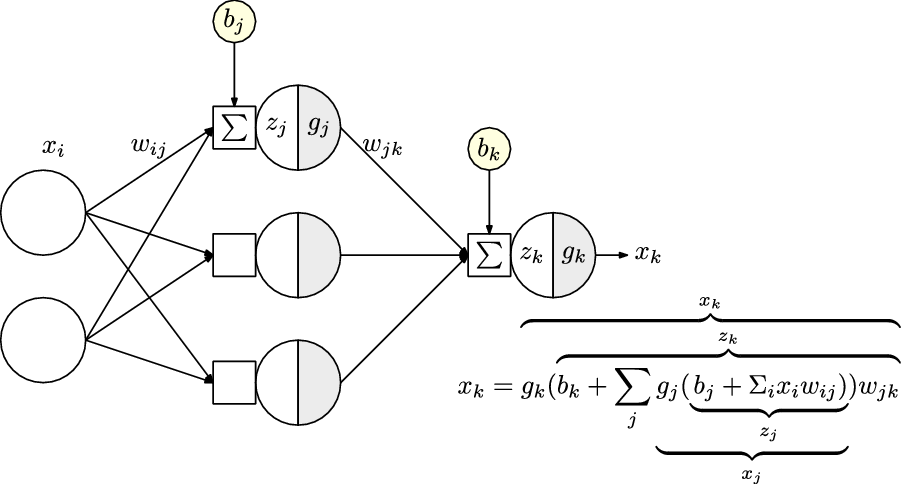
Figure 6. Forward propagation in an artificial neural network with a single hidden layer
Backpropogation: When a neural network is created, the parameters, $\theta$
including the weights and biases, are often initialized randomly or else sampled from a distribution. The prediction of the NN from the forward pass is compared with the true output, computing an error, E, using a loss function. The resultant scalar value indicates how well the parameters of the NN perform the specific task.
$\theta$
including the weights and biases, are often initialized randomly or else sampled from a distribution. The prediction of the NN from the forward pass is compared with the true output, computing an error, E, using a loss function. The resultant scalar value indicates how well the parameters of the NN perform the specific task.
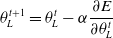
Training a NN involves adjusting the parameters of network $\theta$
, by first computing the derivative of the loss function and then using that information to update the parameters in the direction where the error is reduced. This is called gradient descent. Formally, the parameters are updated as:
$\theta$
, by first computing the derivative of the loss function and then using that information to update the parameters in the direction where the error is reduced. This is called gradient descent. Formally, the parameters are updated as:
 \begin{equation} \theta_{L}^{t+1}=\theta_{L}^{t}-\alpha \frac{\partial E}{\partial \theta_{L}^{t}}\end{equation}
where $\alpha$
is the learning rate. The term
$\alpha$
is the learning rate. The term $\frac{\partial E}{\partial \theta_{L}^{t}}$
represents the partial derivative of the error with respect to the parameters of a layer L. These gradients can be computed by applying chain rule (shown in Figure 7) and involves the gradients of subsequent neurons and layers. Repeated application of chain rule can be used to calculate these gradients at every layer, all the way from the final layer, by navigating through the network backward, hence the name backpropogation (Rumelhart et al., Reference Rumelhart, Hinton and Mcclelland1986). This is a particular case of Automatic Differentiation (Rall, Reference Rall1981).
$\frac{\partial E}{\partial \theta_{L}^{t}}$
represents the partial derivative of the error with respect to the parameters of a layer L. These gradients can be computed by applying chain rule (shown in Figure 7) and involves the gradients of subsequent neurons and layers. Repeated application of chain rule can be used to calculate these gradients at every layer, all the way from the final layer, by navigating through the network backward, hence the name backpropogation (Rumelhart et al., Reference Rumelhart, Hinton and Mcclelland1986). This is a particular case of Automatic Differentiation (Rall, Reference Rall1981).
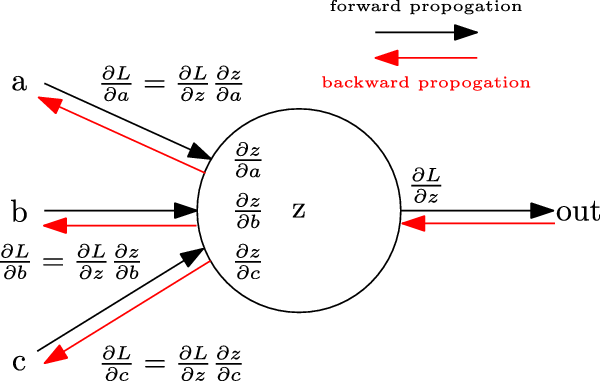
Figure 7. Backpropagation of gradients by application of chain rule
A cost function is another name for a loss function when applied to either the entire training data or a smaller subset known as the batch or mini-batch. Some commonly used cost functions include mean squared error, mean absolute error, cross-entropy, hinge loss, Kullback-Leibler divergence (Kullback & Leibler, Reference Kullback and Leibler1951) etc.
2.4. Activation Function and Weight Initialization
Neural Network (NN) with at least one hidden layer can serve as universal function approximators (Cybenko, Reference Cybenko1989). A NN without an activation function acts like a linear regressor, where the output is a linear combination of its inputs, which restricts its overall learning capacity. An activation function is often used to introduce nonlinearity in the network, which enables it to model much more evolved and complex inputs like images, videos (Ma et al., 2018), audio (Purwins et al., Reference Purwins2019), text (Radford et al., Reference Radford, Wu, Child, Luan, Amodei and Sutskever2019), etc. Some of the widely used nonlinear activation functions are shown in Figure 8.
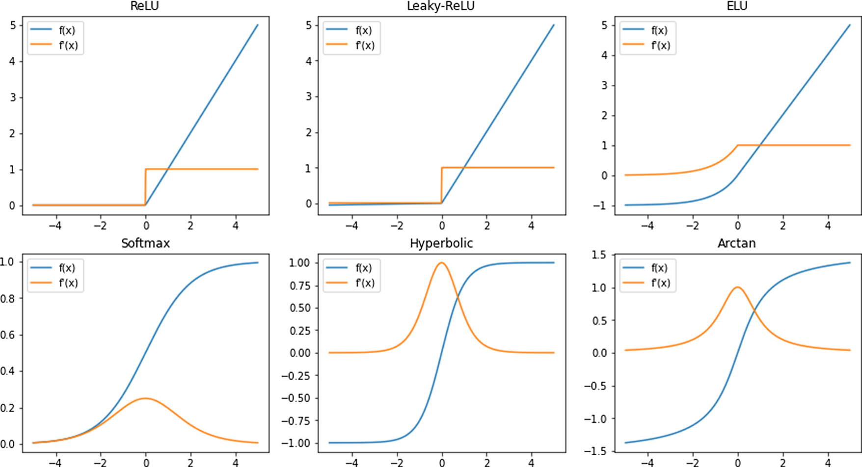
Figure 8. Commonly used activation functions, f(x) and their derivatives, $f^{\,\prime}$
(x) for
$f^{\,\prime}$
(x) for $x \in [\!-5,5]$
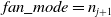
The initialization of the network parameters, primarily the weights and biases of the different layers, plays a critical role when training a neural network. Situations where the activation output and the gradients explode (i.e., become significantly large) or vanish (i.e., become significantly small) due to these parameter values can significantly affect the convergence of the NN as highlighted in Sousa (Reference Sousa2016). Some of the widely used weight initialization strategies and their properties are summarized below:
-
• Normal: The values for the parameters are drawn from a normal distribution,
$\mathcal{N}\!\left(\mu, \sigma^{2}\right)$
, where
$\mu$
is the mean, and
$\sigma^{2}$
is the variance. The probability distribution function for normal distribution is: (24)
\begin{equation} f(x)=\frac{1}{\sigma \sqrt{2 \pi}} e^{-\frac{1}{2}\!\left(\frac{x-\mu}{\sigma}\right)^{2}} \end{equation}
-
• Uniform: The values for the parameters are drawn from a uniform distribution,
$\mathcal{U}(a, b)$
, where a is the lower bound and b is the upper bound for the distribution. The probability distribution function for continuous uniform distribution is: (25)
\begin{equation} f(x)=\left\{\begin{array}{l@{\quad}l} \frac{1}{b-a} & \text { for } a \leq x \leq b, \\ \\[-8pt] 0 & \text { for } xb \end{array}\right. \end{equation}
-
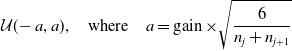
• Xavier: This is also known as Glorot initialization (Glorot & Bengio, Reference Glorot and Bengio2010) and overcomes the problem of vanishing, exploding gradients by adjusting the variance of the weights. Xavier uniform initialization samples the weight matrix, W, between the layer j and
$j+1$
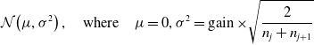
from a uniform distribution. (26)The parameter gain is an optional scaling factor and, n is the number of neurons of the respective layer. Xavier normal initialization draws samples from a normal distribution.
\begin{equation} \mathcal{U}(\!-a,a), \quad\text{where}\quad a=\operatorname{gain} \times \sqrt{\frac{6}{n_j+n_{j+1}}} \end{equation}
(27)
\begin{equation} \mathcal{N}\!\left(\mu, \sigma^{2}\right), \quad\text{where}\quad \mu=0, \sigma^{2} = \operatorname{gain} \times \sqrt{\frac{2}{n_j+n_{j+1}}} \end{equation}
-
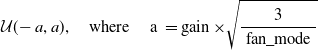
• Kaiming: This is also known as He initialization (He et al., Reference He2015b), and is well suited for NN with asymmetric and nonlinear activation functions, for example, ReLU, Leaky-ReLU, ELU, etc. Kaiming uniform initialization samples the weight matrix, W, between the layer j and
$j+1$
from a uniform distribution. (28)The parameter gain is an optional scaling factor, and
\begin{equation} \mathcal{U}(\!-a,a), \quad\text{where}\quad \text { a }=\operatorname{gain} \times \sqrt{\frac{3}{\text { fan_mode }}} \end{equation}
${\text { fan_mode }}$
is the number of neurons of the respective layer.
${\text { fan_mode }}=n_{j+1}$
preserves the magnitude of the variance for the weights during the backward pass whereas,
${\text { fan_mode }}=n_{j}$
preserves it in the forward pass. Kaiming normal initialization draws samples from a normal distribution. (29)
\begin{equation} \begin{aligned} \mathcal{N}\!\left(\mu, \sigma^{2}\right), \quad\text{where}\quad \mu=0, \mathrm{std} & = \frac{\text { gain }}{\sqrt{\text { fan_mode }}} \end{aligned} \end{equation}


2.5. Evolutionary computation
EC draws inspiration from nature and utilizes the same concepts to solve computational problems. This family of algorithms has its root spread out in computer science, artificial intelligence as well as evolutionary biology, Figure 9.

Figure 9. Evolutionary computation has its roots within computer science, artificial intelligence and evolutionary biology
EC belongs to a class of population-based optimization techniques where a set of solutions are generated and iteratively updated through genetic operators. A new generation of solutions is produced by stochastically eliminating ‘less fit’ solutions and introducing minor random variations in the population. At a high level, it is simply adapting to the changes within the environment by means of small random changes. The combined use of EC and DL has led to very auspicious results on several complex engineering tasks and drawn great academic interest (Salimans et al., Reference Salimans2017; Conti et al., Reference Conti, Madhavan, Such, Lehman, Stanley and Clune2018).
EC consists of several meta-heuristic optimization algorithms, some of which are explained in the following subsections.
2.5.1. Genetic algorithm
GAs, first developed in 1975 (Holland, Reference Holland1992a), is a widely used class of evolutionary algorithms (Mitchell, Reference Mitchell1996) that takes inspiration from Charles Darwin’s theory of evolution (Darwin, Reference Darwin1859). It is meta-heuristic-based optimization technique that follows the principle of ‘survival of the fittest’.
The key components of any GA (Mitchell, Reference Mitchell1996) are:
-
• Population: is the subset of all possible solutions to a problem. Every GA starts with an initialization of a set of solutions that become the first population. Each solution, individual from the population, is known as a chromosome which consists of several genes.
-
• Genotype: is the representation of the individuals of a population in the computation space. This is done to ensure efficient processing and manipulation by the computing system.
-
• Phenotype: is the actual representation of the population in the space of solutions.
-
• Encoding and Decoding: For more straightforward problems, the genotype and the phenotype may be the same. However, complex problems rely on a translation mechanism to encode a phenotype to a genotype and a decoder for the reverse task.
-
• Fitness function: is a tool to measure the performance of an individual on a specific problem.
-
• Genetic operators: are tools utilized by the algorithm to produce a new set of solutions from the existing ones.
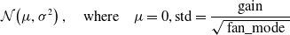
The algorithm starts by initializing a set of solutions, the population, which is also known as a generation. At each iteration, the fitness function is used to evaluate the performance of the entire population. The solutions with higher fitness (Baluja & Caruana, Reference Baluja and Caruana1995) are stochastically selected as the parents of the current generation. Genetic operators are applied to the parents to generate the next generation. This process is repeated until the required level of fitness is achieved. The complete workflow of a simple GA is shown in Figure 10.
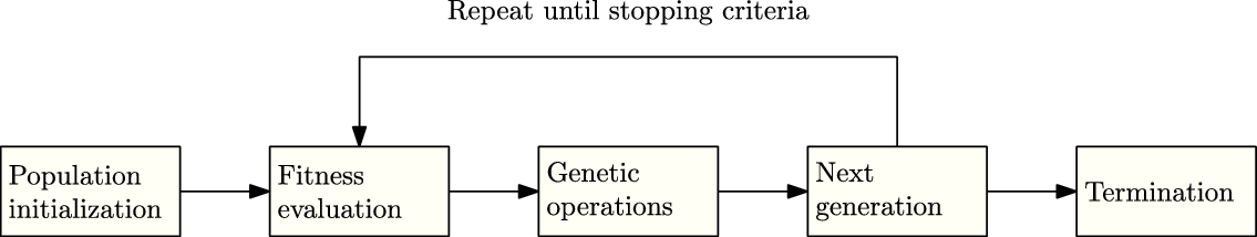
Figure 10. Workflow of a simple genetic algorithm
The genetic operators are fundamental components of this algorithm that guides it toward a solution. The widely used genetic operators are summarized in the following subsections.
Selection Operators: The selection operator uses the fitness values as a measure of performance and picks a subset of the population as the current generation’s parents. A common strategy is to assign a probability value proportional to the fitness scores, with the goal that more fit individuals have a higher chance of being selected. Some other strategies include random selection, tournament selection, and roulette wheel selection, proportionate selection, steady-state selection, etc. (Haupt & Haupt, Reference Haupt and Haupt2003). The best performing individual from the current generation is selected and carried to the next generation without any alterations. This strategy is known as elitism (Baluja & Caruana, Reference Baluja and Caruana1995) and ensures that performance does not decrease over iterations.
Crossover operator: This operator picks a pair from the solutions shortlisted by the selection operator. The selected pair then mates and generates new solutions, which are known as the offspring. Each offspring is produced stochastically and contains genetic information, that is, features from either parent which is analogous to the crossover of genes in biology.
Single-point crossover is a commonly used crossover operator. A random crossover point is picked on the encoding of both parents. The offspring are then produced by recombination of the left partition of one parent with the right split of the other and vice versa. The same strategy can be extended to more than one crossover point. Figure 11 shows single-point crossover and two-point crossover between two binary encoded parents. In situations, where the encoding is an ordered list (Larranaga et al., Reference Larranaga1999), the solutions generated with the methods mentioned above, may be invalid. To overcome such issues, specialized operators like order crossover (Larranaga et al., Reference Larranaga1996), cycle crossover (CX) (Larranaga et al., Reference Larranaga1999) and partially mapped crossover have been published.
Figure 11. Single-point crossover (top) and two-point crossover (bottom) between two parents to generate offsprings for the next generation
Mutation operator: The mutation operator makes small arbitrary changes to an individual or its encoded representation which promotes the algorithm to explore the search space and find new solutions. As a result, the diversity within the population is improved during successive generations, and the algorithm can avoid getting stuck at local minima. Some commonly used mutation operators include Gaussian operators, uniform operators, bit flip operators (binary encoding), and shrink operators (Da Ronco & Benini, Reference Da Ronco, Benini and Kim2014). These operators are applied with a relatively small probability known as the mutation rate and have a few hyperparameters that can be tuned to specific problems.
2.5.2. Evolution strategies
Evolution Strategy (ES) is a black-box optimization technique that draws inspiration from the theory of natural selection, a process in which individuals from a population adapt to the changes of the environment.
Consider a 2D function, $f\,{:}\, \mathbb{R}^{2} \rightarrow \mathbb{R}$
, for which the gradient,
$f\,{:}\, \mathbb{R}^{2} \rightarrow \mathbb{R}$
, for which the gradient, $\nabla f\,{:}\, \mathbb{R}^{n} \rightarrow \mathbb{R}^{n}$
, can not be computed directly, and we wish to obtain the parameters
$\nabla f\,{:}\, \mathbb{R}^{n} \rightarrow \mathbb{R}^{n}$
, can not be computed directly, and we wish to obtain the parameters $x^*$
and
$x^*$
and $y^*$
, such that
$y^*$
, such that $f(x^*,y^*)$
is the global maximum. The ES algorithm starts with a set of solutions for the problem, which are sampled from a parameterized distribution. An objective function then evaluates each solution and returns a single value as a fitness metric which is then utilized to update the parameters of the distribution.
$f(x^*,y^*)$
is the global maximum. The ES algorithm starts with a set of solutions for the problem, which are sampled from a parameterized distribution. An objective function then evaluates each solution and returns a single value as a fitness metric which is then utilized to update the parameters of the distribution.
Gaussian Evolution Strategy: One of the simplest techniques is to sample from a normal distribution, $\mathcal{N}\!\left(\mu, \sigma^{2}\right)$
, where
$\mathcal{N}\!\left(\mu, \sigma^{2}\right)$
, where $\mu$
is the mean and
$\mu$
is the mean and $\sigma^2$
is the variance. For the function defined above, one could start with
$\sigma^2$
is the variance. For the function defined above, one could start with $\mu=(0,0)$
and some constant,
$\mu=(0,0)$
and some constant, $\sigma=(\sigma_x,\sigma_y)$
. After one generation, the mean can be updated to the best performing solution from the population. Such a naive approach is only applicable to simple problems and also prone to getting stuck at local minima since it is greedy with respect to the best solution at each step of the training process.
$\sigma=(\sigma_x,\sigma_y)$
. After one generation, the mean can be updated to the best performing solution from the population. Such a naive approach is only applicable to simple problems and also prone to getting stuck at local minima since it is greedy with respect to the best solution at each step of the training process.
Covariance Matrix Adaptation Evolution Strategy: The simple Gaussian strategy explained above assumes a constant variance. In some applications, it is worthwhile to explore the search space by having a larger variance initially and fine-tuning it later on when we are close to a good solution. Covariance-Matrix Adaptation Evolution Strategy (CMA-ES) samples the solutions from a multivariate Gaussian distribution. It then adapts both the mean as well as the covariance matrix from the fitness metrics of the solutions. This algorithm is widely applicable to non-convex and nonlinear optimization problems (Hansen & Auger, Reference Hansen and Auger2011), especially in the continuous domain. There is no need to tune the parameters for a specific application since optimizing the parameters is incorporated within the design of this algorithm.
Natural Evolution Strategy: Simple Gaussian ES and CMA-ES both have the identical drawback of utilizing only the best individuals from the population and discarding all the others. At times, it might be beneficial to incorporate the information from low-scoring individuals as well, since they contain the vital information of what not to do. Natural Evolution Strategy (NES) (Wierstra et al., Reference Wierstra2008) utilize the information from the entire population to estimate the gradients, which are utilized to update the distribution from which the solutions were sampled. For an objective function, F with parameters $\theta$
which are sampled from a parameterized distribution
$\theta$
which are sampled from a parameterized distribution $p_\psi(\theta)$
. The algorithm’s goal is to optimize the average objective
$p_\psi(\theta)$
. The algorithm’s goal is to optimize the average objective $\mathbb{E}_{\theta \sim p_{\psi}}[F(\theta)]$
. The parameters of the distribution are iteratively updated using stochastic gradient ascent. The gradient of the objective is computed as follows:
$\mathbb{E}_{\theta \sim p_{\psi}}[F(\theta)]$
. The parameters of the distribution are iteratively updated using stochastic gradient ascent. The gradient of the objective is computed as follows:
 \begin{align} \nabla_{\psi}\!\left(\mathbb{E}_{\theta \sim p_{\psi}}[F(\theta)]\right) & =\nabla_{\psi}\!\left(\int_{\theta} p_{\psi}(\theta) \cdot F(\theta) \cdot d \theta\right) \nonumber\\ & =\int_{\theta} \nabla_{\psi}\!\left(p_{\psi}(\theta)\right) \cdot F(\theta) \cdot d \theta \nonumber\\ &=\int_{\theta} p_{\psi}(\theta) \cdot \nabla_{\psi}\!\left(\log p_{\psi}(\theta)\right) \cdot F(\theta) \cdot d \theta \nonumber\\ & =\mathbb{E}_{\theta\sim p_{\psi}}\!\left[\nabla_{\psi}\!\left(\log p_{\psi}(\theta)\right) \cdot F(\theta)\right] \end{align}
Equation: 30 uses the same log-likelihood technique as the popular reinforce algorithm (Sutton & Barto, Reference Sutton and Barto2018). The expectation can be computed using Monte Carlo approximations by sampling points as shown in Equation (31).
 \begin{equation}\begin{aligned}\nabla_{\psi}\!\left(\mathbb{E}_{\theta \sim p_{\psi}}[F(\theta)]\right) &=\mathbb{E}_{\theta\sim p_{\psi}}\!\left[\nabla_{\psi}\!\left(\log p_{\psi}(\theta)\right) \cdot F(\theta)\right] \\[3pt] & \approx \frac{1}{\lambda} \sum_{k=1}^{\lambda} \!\left[\nabla_{\psi}\!\left(\log p_{\psi}(\theta)\right) \cdot F(\theta)\right]\end{aligned}\end{equation}
Evolution Strategy for RL: Researchers in Salimans et al. (Reference Salimans2017) utilized Natural Evolution Strategy to find the optimal parameters of a neural network for RL problems. The parameters represent the weights and biases, and the objective is the stochastic return from the environment. The parameterized distribution, $p_\psi(\theta)$
is assumed to be multivariate gaussian with mean
$p_\psi(\theta)$
is assumed to be multivariate gaussian with mean $\psi$
and a fixed noise of
$\psi$
and a fixed noise of $\sigma^2I$
.
$\sigma^2I$
.
 \begin{equation}\theta \sim \mathcal{N}\!\left(\psi, \sigma^{2} I\right) \text { equivalent to } \theta=\psi+\sigma \epsilon, \epsilon \sim \mathcal{N}(0, I)\end{equation}
This parametrization allows to rewrite the average objective as $\mathbb{E}_{\theta \sim p_{\psi}} F(\theta)=\mathbb{E}_{\epsilon \sim N(0, I)} F(\theta+\sigma \epsilon)$
. Given the revised definition of the objective function, the authors derive (Salimans et al., Reference Salimans2017) the gradient of the objective function in terms of
$\mathbb{E}_{\theta \sim p_{\psi}} F(\theta)=\mathbb{E}_{\epsilon \sim N(0, I)} F(\theta+\sigma \epsilon)$
. Given the revised definition of the objective function, the authors derive (Salimans et al., Reference Salimans2017) the gradient of the objective function in terms of $\theta$
as
$\theta$
as
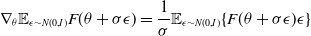 \begin{equation}\nabla_{\theta} \mathbb{E}_{\epsilon \sim N(0, I)} F(\theta+\sigma \epsilon)=\frac{1}{\sigma} \mathbb{E}_{\epsilon \sim N(0, I)}\{F(\theta+\sigma \epsilon) \epsilon\}\end{equation}
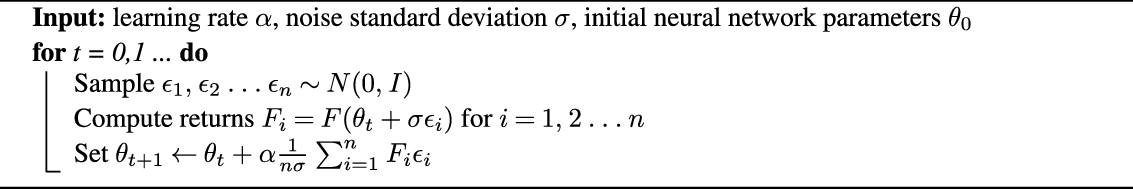
The gradients are approximated by generating samples of noise $\epsilon$
during training and the parameters are then optimized using stochastic gradient ascent as shown in Algorithm 1.
$\epsilon$
during training and the parameters are then optimized using stochastic gradient ascent as shown in Algorithm 1.
Algorithm 1: Evolution strategy for RL by OpenAI (Salimans et al., Reference Salimans2017)
2.5.3. Neuroevolution
Neuroevolution is a form of Artificial Intelligence (AI) that combines EC with NNs. The objective is to either learn the topology of the NN or its parameters, that is, weights and biases by utilizing algorithms discussed in Sections 2.5.1 and 2.5.2.
An individual within the population is a NN or its parameters—weights and biases. The trivial method of storing a NN, as a complex data structure, in the parameter space scales poorly in memory, especially with the increasing population size, and makes the application of genetic operators a computationally expensive task. Hence, the need for simplified encoding of the NN.
Direct encoding: In the notable work, ’Evolving neural networks through augmenting topologies’, NEAT (Stanley & Miikkulainen, Reference Stanley and Miikkulainen2002), the authors propose a direct encoding wherein the connections between each neuron are explicitly stored with all the weights and biases, as shown in Figure 12. Such an encoding gives a very high degree of flexibility to the network topology but has a massive search space due to a fine granularity of the encoding. This approach is not well suited for DNN, which consists of several hidden layers, each with thousands of neurons.

Figure 12. A simplified version of direct encoding proposed in NEAT (Stanley & Miikkulainen, Reference Stanley and Miikkulainen2002). Mapping of genotype, a neural network to a phenotype, its encoding
Indirect encoding: This type of encoding relies on a translation function or a mechanism that maps a neural network to its encoded representation. Unlike, direct encoding which is a quick way to encode or decode a neural network, this type of encoding has a processing overhead and limited granularity. Some implementations that employ an indirect encoding include Compositional Pattern Producing Networks (CPPNs) (Stanley, Reference Stanley2007), HyperNEAT (Stanley et al., Reference Stanley, D’Ambrosio and Gauci2009) and Deep Neuroevolution (Conti et al., Reference Conti, Madhavan, Such, Lehman, Stanley and Clune2018).
2.6. Related work
Computing the Q-value for complex problems with a large state-action space using traditional tabular RL algorithms is computationally infeasible. This led to the use of function approximations like neural networks for estimating the Q-values (Melo et al., Reference Melo, Meyn and Ribeiro2008), which is memory efficient and can also be applied to problems with continuous state and action spaces (Van Hasselt, Reference Van Hasselt2013).
The first significant breakthrough in deep reinforcement learning, the combined use of deep learning and reinforcement learning, was the introduction of DQN (Mnih et al., Reference Mnih and Kavukcuoglu2015) which incorporated two critical components in the training process, an experience replay buffer and a separate target network. The replay memory stores the agent’s experience, including the states, actions and rewards over a few episodes and the target network is a periodically updated copy of the main network which is used to decide what actions to perform. During training, samples are drawn from the replay memory to remove the correlations between the observations. The combined use of these two innovative techniques stabilized the learning of Q-values and achieved state-of-the-art performance on many Atari 2600 benchmarksFootnote 5.
Over the past few years, several extensions to DQN have been proposed. A known problem with Q-learning is its tendency to overestimate the targets since it relies on a single estimator for the Q-values. A technique called Double Q-learning (Hasselt, Reference Hasselt2010) tries to rectify this issue by utilizing a double estimator. An extension of DQN with double estimators, was implemented in Double DQN (van Hasselt et al., Reference van Hasselt, Guez and Silver2016). When sampling from the replay buffer as proposed in DQN, all samples, that is, transitions were given the same significance. Research on a prioritized experience replay (Schaul et al., Reference Schaul, Quan, Antonoglou and Silver2015) that offered a higher importance to more frequent transitions resulted in improved performance and was included in most subsequent research. A Dueling network architecture (Wang et al. Reference Wang, Schaul, Hessel, Hasselt, Lanctot and Freitas2016) with two estimators—one for Q-values and the other for state-dependent action advantage function, was proposed and shown to have better generalization properties. Deep Deterministic Policy Gradient (DDPG) (Lillicrap et al., Reference Lillicrap2015) combines the use of deterministic policy gradient and DQN and can be operated on a continuous action space making its application particularly useful in robotics (Dong & Zou, Reference Dong and Zou2020).
The slow rate of convergence and longer duration of training prompted the need for parallelizable algorithms. A distributed framework for RL, Gorilla (Nair et al., Reference Nair, Srinivasan, Blackwell, Alcicek, Fearon, De Maria, Panneershelvam, Suleyman, Beattie, Petersen and Legg2015) was proposed by researchers at Google which consists of several actors, all learning continuously in parallel and syncing their local gradients with a global parameter server after a few steps. This parallelized variant of DQN outperformed its standard counterpart on several benchmarks and reduced the training time.
Asynchronous Advantage Actor Critic (A3C) (Mnih et al., Reference Mnih, Badia, Balcan and Weinberger2016) is a parallelized policy gradient method that consists of several agents, independently interacting with copies of environments in parallel. The algorithm consists of one global network with shared parameters and uses asynchronous gradient descent for optimization. In Asynchronous Advantage Actor Critic (A3C), each agent communicates with the global network independently. The aggregated policy from different agents, when combined together may not be optimal. A2C (Mnih et al., Reference Mnih, Badia, Balcan and Weinberger2016) is deterministic and synchronous version of A3C, which resolves this inconsistency by using a coordinator that ensures a synchronous communication between agents and global network.
2.6.1. Evolution-based RL
The Q-learning-based methods try to solve the Bellman optimality equation whereas, policy gradient algorithms consist of parameterizing the policy itself to learn the probability of taking an action in a state. Regardless, they usually entail expensive computations, such as gradient calculations and back-propagation, which result in very lengthy (i.e., hours to even days) training in order to obtain desirable results, especially when solving complex problems with large state spaces (Lillicrap et al., Reference Lillicrap2015; Mnih et al., Reference Mnih and Kavukcuoglu2015; Mnih et al., Reference Mnih, Badia, Balcan and Weinberger2016).
Recently we see a surge of a number of alternative approaches to solving RL problems, including the use of EC. These methods have been quite effective in discovering high-performing policies (Whiteson, Reference Whiteson2012). A notable contribution is the work by OpenAI on Evolution Strategy (ES) (Salimans et al., Reference Salimans2017) to train deep neural networks. ES does not calculate the gradients analytically, instead approximate the gradient of the reward function in the parameter space using minor random tweaks. This massively scalable algorithm, trained on several thousand workers was able to solve the 3D humanoid walking benchmark (Tassa et al., Reference Tassa, Erez and Todorov2012) within minutes and also outperformed several established deep reinforcement learning algorithms on many complex robotic control tasks and Atari 2600 benchmarks. Collaborative Evolutionary Reinforcement Learning (CERL) (Khadka et al., Reference Khadka, Majumdar, Chaudhuri and Salakhutdinov2019) is another scalable framework that was designed to simultaneously explore different regions of the search space and creating a portfolio of policies, the results on continuous control benchmarks highlighted improved sample efficiency of such approaches. Another breakthrough work by researchers at UberAI, is Deep Neuroevolution (Conti et al., Reference Conti, Madhavan, Such, Lehman, Stanley and Clune2018), a black-box optimization technique based on principles of evolutionary computation. Deep Neuroevolution utilizes a simple GA to train a convolutional neural network that approximates the Q-function.
Results from these publications highlight improved performance and significant speedup due to distributed training (Salimans et al., Reference Salimans2017; Conti et al., Reference Conti, Madhavan, Such, Lehman, Stanley and Clune2018). Moreover, these gradient-free approaches can be applied to non-differentiable domains (Cho et al., Reference Cho2014; Xu et al., Reference Xu2016; Liu et al., Reference Liu2018) and for training models that require low precision arithmetic—binary neural networks on low precision hardware. In a subsequent paper (Conti et al., Reference Conti, Madhavan, Such, Lehman, Stanley and Clune2018), the same researchers incorporated quality diversity (QD) (Cully et al., Reference Cully2015; Pugh et al., Reference Pugh, Soros and Stanley2016) and novelty search (NS) (Lehman & Stanley, Reference Lehman and Stanley2008) to ES, and proposed three different algorithms, which improved performance and also directed the exploration. Their work also highlighted the algorithm’s robustness against a local minima.
Several population-based evolutionary algorithms have been used to train neural networks or optimize their architecture (Jaderberg et al., Reference Jaderberg2017) and the hyperparameters (Liu et al., Reference Liu2017), but a rather interesting approach was proposed in Genetic Policy Optimization (GPO) (Gangwani & Peng, Reference Gangwani and Peng2018) algorithm which utilized imitation learning as crossover and policy gradient techniques for mutations. The algorithm had superior performance and improved sample efficiency in comparison to known policy gradient methods. Evolutionary Reinforcement Learning (ERL) (Khadka & Tumer, Reference Khadka and Tumer2018) is another hybrid approach that uses a population-based optimization strategy guided by policy gradients for challenging control problems.
3. Species-based Genetic algorithm (Sp-GA)
A typical GA (Section 2.5.1) consists of a population of individuals where each individual is a potential solution to the problem. In the context of RL, a solution may represent a policy, a neural network that estimates the Q-function (Mnih et al., Reference Mnih and Kavukcuoglu2015) or a neural network that predicts what action to take given the state as an input. In this work, we propose a GA wherein each individual is a neural network that estimates the Q-function for the specific RL problem. The algorithm initializes the population of such neural networks from a species-based initialization routine and iteratively evolves the population to search for the best solution. We call this algorithm Sp-GA.
3.1. Species initialization
The notion of speciation was first investigated in NEAT (Stanley & Miikkulainen, Reference Stanley and Miikkulainen2002), which clustered neural networks with similar topologies into subclasses called species. The philosophy behind the approach is to give sufficient time for evolution to new solutions within a smaller subset before they compete with other species. As a result, innovation, novelty, and diversity are protected within the population.
Sp-GA extends the concept of speciation to the weight initialization strategy of a neural network. The initialization of weights is a critical design choice that can adversely affect the network’s rate of convergence (He et al., Reference He2015b; Sousa, Reference Sousa2016). The choice of initialization sets the starting point of the optimization process and therefore controls the effectiveness of training. The algorithm maintains a pool of such strategies, each having unique properties and particular advantages. When the population is initialized, a neural network is assigned a species uniformly at random, and the weights are initialized as per the strategy for that species. Figure 13 shows the distribution of individuals, that is, neural networks initialized from the proposed methodology wherein five weight initialization strategies were utilized.

Figure 13. Distribution of species in a population of size 200. Each species is a unique weight initialization strategy for neural networks
3.2. Algorithm hyperparameters
The proposed algorithm has the following hyperparameters:
-
1. Population size (N): controls the number of neural networks in the population. This is an important parameter that controls the search space to find the solution. For more straightforward problems like CartPole from gym environment even a small value
$N\approx50$
gave good results. For more complex problems like the ones addressed in this work, a higher number is preferred. -
2. Mutation Power (
$\sigma$
): controls the strength of mutation, that is, the perturbations applied to the parameters of the neural network. This operator is responsible for exploration of better solutions in the search space. In case of Gaussian operator, it is the variance of the distribution. A small value between 0.001
$\sim$
0.003 showed promising results. -
3. Fraction/Number of elites ( E ): control the number of neural networks shortlisted as parents of the current generation and are responsible for producing the next generation. This parameter is responsible for preserving the best performing solution of a generation.
-
4. Mutation probability (
$\psi$
): represents the probability of using the mutation operator. Conversely, 1-
$\psi$
is the probability of using the crossover operator. -
5. Number of species ( S ): is the number of species spawned in the population. Each species corresponds to a weight initialization strategy of a neural network. During initialization, each neural network is assigned a particular species uniformly at random. The choice of initialization sets the starting point of the optimization process and therefore controls the effectiveness of training.


The pseudocode for Sp-GA is shown in Algorithm 2. The algorithm starts with the initialization of a population P, neural networks, with S different species. Each network is an estimator of the Q-function for the RL problem. The next step is to evaluate the fitness of the entire population. The fitness value of a single neural network is estimated by calculating the cumulative return for a fixed time horizon in the simulated environment. Once the fitness values are evaluated, a fraction of neural networks E, with the highest scores, are selected as the parents of the current generation. The parents then generate the offspring, using genetic operators as explained in Section 3.3.2 to form the new generation. The process is then repeated until the stopping criteria.
Algorithm 2: Species-based genetic algorithm (Sp-GA)
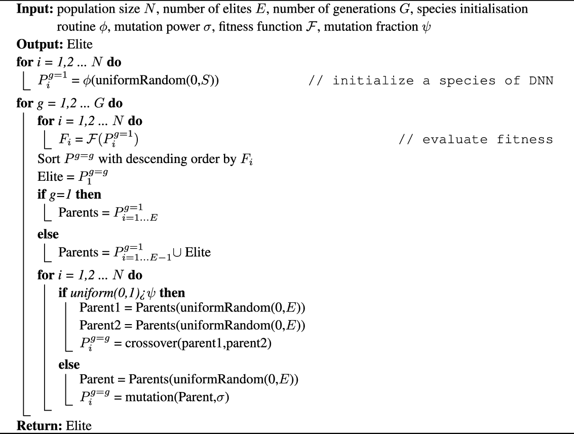
3.3. Distributed Sp-GA
A unique advantage of a GA is its ability to evaluate the fitness of the individuals in parallel, making it suitable for a distributed computation. A master-worker segregates the population into smaller subsets which are then sent to slave workers for fitness evaluation. These slave workers can work independently in parallel and return the scalar fitness scores back to the master-worker for the subsequent steps of the algorithm.
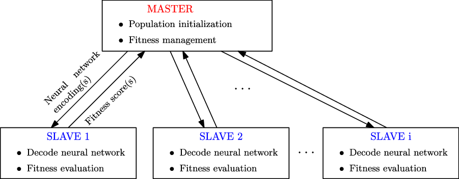
Figure 14. Distributed framework for Sp-GA
Such a naive approach cannot be directly applied to Sp-GA due to several reasons. A large population size would involve sending a lot of neural networks back and forth between workers over a network. A typical deep neural network that is stored as a complex data structure (or an object) takes a few megabytes of memory (Conti et al., Reference Conti, Madhavan, Such, Lehman, Stanley and Clune2018) and is not trivially serializable. This would result in a high memory and bandwidth requirement for the communication.
Distributed Sp-GA relies on an encoding mechanism that takes inspiration from Deep Neuroevolution (Conti et al., Reference Conti, Madhavan, Such, Lehman, Stanley and Clune2018). The encoding of a neural network scales well with memory, can be serialized and therefore utilizes low bandwidth making it ideal for distributed training. This encoding also enables an intuitive application of genetic operators like mutation as well as crossover which was not implemented in the previous work (Salimans et al., Reference Salimans2017; Conti et al., Reference Conti, Madhavan, Such, Lehman, Stanley and Clune2018).
Figure 14 shows the distributed framework implemented in Sp-GA. The pipeline can be summarized as:
-
1. The master-worker first initializes the population—a set of NNs. It is responsible for encoding these networks and creating a mapping dictionary.
-
2. During training, the master sends an encoded neural network (or a subset) to the slave workers.
-
3. A slave worker decodes the encoding to produce the complete neural network, evaluate its fitness and returns a scalar value, the fitness score, back to the master-worker.
-
4. Once the fitness values of the entire population are available, the subsequent steps of the Algorithm 2 are carried out by the master-worker.
3.3.1. Model encoding
An individual from the population which is a neural network, is stored as list of tuples, as shown in Figure 15.
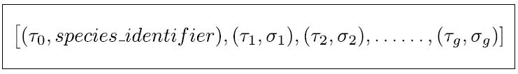
Figure 15. Proposed encoding of a neural network
The first tuple consists of a randomly selected seed utilized for initializing the model parameters, and the second entry is the identifier for the species of the network. Every subsequent tuple consists of another seed value and the mutation power ( $\sigma$
) utilized by the genetic operators for training the network parameters.
$\sigma$
) utilized by the genetic operators for training the network parameters.
3.3.2. Genetic operators in encoded space
The Gaussian operator is the choice for mutation in this work. Given a neural network with parameters, $\theta$
, the Gaussian operator updates all the parameters as:
$\theta$
, the Gaussian operator updates all the parameters as:
 \begin{equation} \theta^{\prime}=\theta+\sigma \epsilon\end{equation}
where $\epsilon \sim \mathcal{N}(0, I)$
and where
$\epsilon \sim \mathcal{N}(0, I)$
and where $\sigma$
is the mutation power. If a parent is selected for mutation, the encoding of the resultant network is simply the original encoding appended with a new tuple containing the seed and the mutation power. This process is shown in Figure 16. When needed, any encoding can be decoded to the actual network by iteratively setting the seed and applying the Gaussian mutations.
$\sigma$
is the mutation power. If a parent is selected for mutation, the encoding of the resultant network is simply the original encoding appended with a new tuple containing the seed and the mutation power. This process is shown in Figure 16. When needed, any encoding can be decoded to the actual network by iteratively setting the seed and applying the Gaussian mutations.
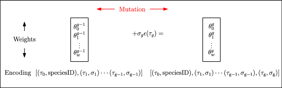
Figure 16. Mutation of a neural network in parameter and encoded space. $\theta_{0:w}^{g-1}$
represent the parameters of the network at
$\theta_{0:w}^{g-1}$
represent the parameters of the network at $g-1$
generation.
$g-1$
generation. $\theta_{0:w}^g$
are obtained by utilizing a gaussian operator with
$\theta_{0:w}^g$
are obtained by utilizing a gaussian operator with $\sigma_g$
as the mutation power and
$\sigma_g$
as the mutation power and $\tau_g$
as the random seed
$\tau_g$
as the random seed
The proposed encoding is also well suited for the application of single-point crossover as described in Section 2.5.1. A random point on the encoded representation of the parents is chosen as the crossover point. A new offspring is produced by merging the left and right partitions (and vice versa) of either parent. The resulting list represents a valid encoding of a neural network. Figure 17 shows this intuitive application of crossover. This approach can also be applied to neural networks with different architectures and took inspiration from the crossover of chromosomes in genetics.
4. Implementation
4.1. Hardware and Software
The entire code was written in Python version 3.8.7. The critical libraries utilized for the implementation are summarized in Table 1.
Table 1. Some key libraries used for the experiments

The development was done within a dockerized environment, and training was performed on a Kubernetes cluster. The quota allocated to this project was limited to 50 CPUs and a memory of 200GB. No GPU was utilized in any experiment. Reference implementations for DQN, A3C, and ES were obtained from rllib package in the ray library.
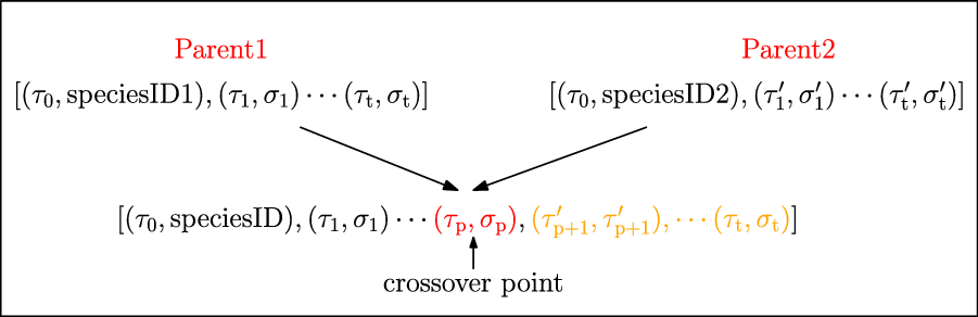
Figure 17. Crossover of two neural networks in encoded space
4.2. Models
Two deep neural networks are implemented from scratch for the conducted experiments.
4.2.1. Model 1
Model 1 is used as the neural network for all Atari 2600 games. This includes Experiments 1, 2, 3, and 4. The architecture of the model is identical to DQN (Mnih et al., Reference Mnih, Badia, Balcan and Weinberger2016). The model takes the preprocessed training frame of size $84\times84\times4$
as the input and outputs the Q-value for all possible actions for that game. There are three layers of convolution. The first convolution layer has 32 filters of size
$84\times84\times4$
as the input and outputs the Q-value for all possible actions for that game. There are three layers of convolution. The first convolution layer has 32 filters of size $8\times8$
, which are applied with a stride of 4 and ReLU activation function. The second convolution layer has 64 filters of size
$8\times8$
, which are applied with a stride of 4 and ReLU activation function. The second convolution layer has 64 filters of size $4\times4$
, which are applied with a stride of 2 and ReLU activation. The last convolution layer has 64 filters of size
$4\times4$
, which are applied with a stride of 2 and ReLU activation. The last convolution layer has 64 filters of size $3\times3$
, which are applied with a stride of 1 and ReLU activation. The penultimate layer is fully connected with an output of 512 neurons. The final output layer is a fully connected layer with the output neurons equivalent to the possible actions in the game. The architecture of the model is shown in Figure 18. The model consists of over 1.7M trainable parameters and has a size of about 6.75MB.
$3\times3$
, which are applied with a stride of 1 and ReLU activation. The penultimate layer is fully connected with an output of 512 neurons. The final output layer is a fully connected layer with the output neurons equivalent to the possible actions in the game. The architecture of the model is shown in Figure 18. The model consists of over 1.7M trainable parameters and has a size of about 6.75MB.
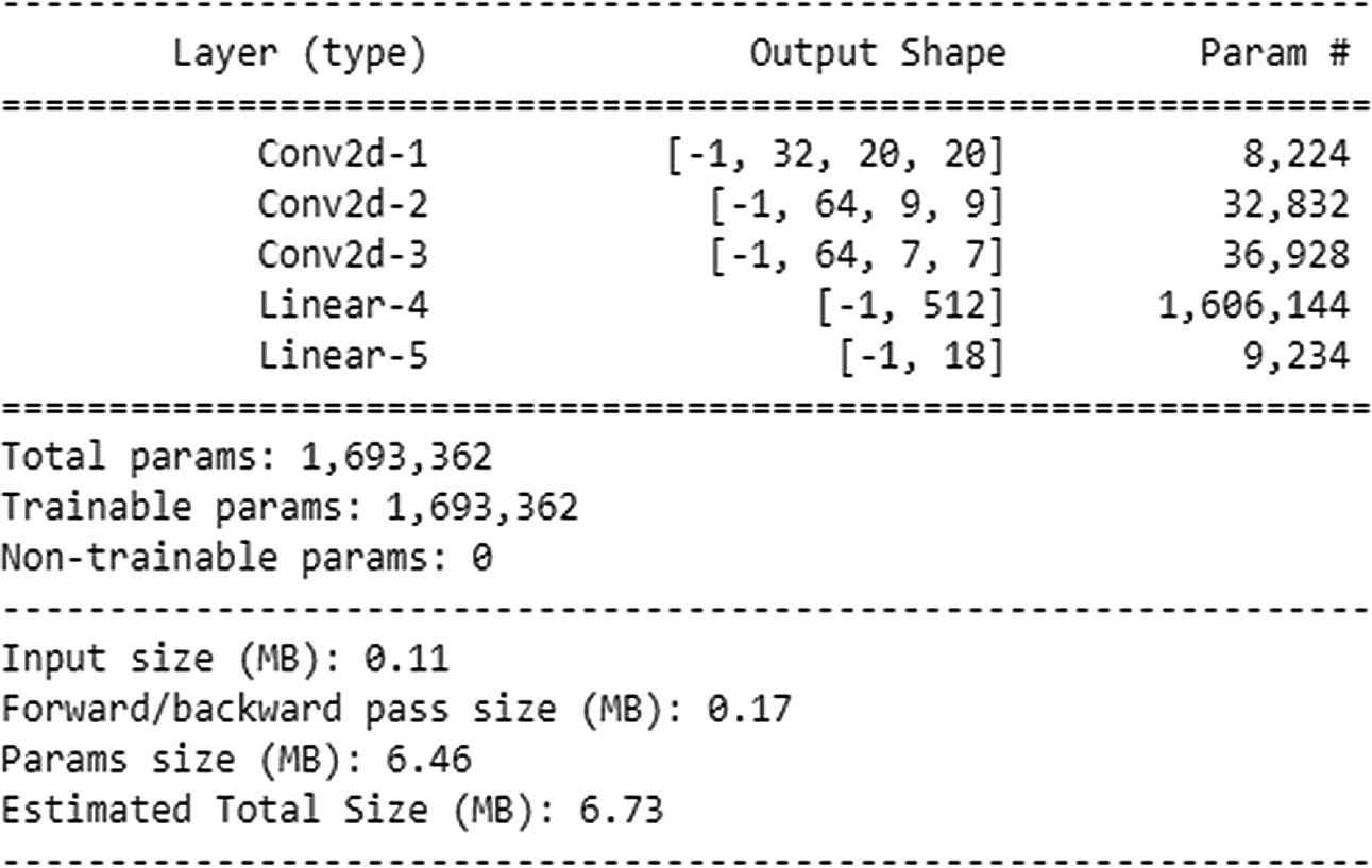
Figure 18. Neural network used for Atari 2600 games
4.2.2. Model 2
Model 2 is used as the neural network for the Remote Electrical Tilt (RET) simulator by Ericsson, that is, Experiment 5. It is a feed-forward network with four fully connected layers of size 100, 50, 20, and 3 respectively. The architecture of the model is shown in Figure 19. This model has over 7500 trainable parameters and a size of about 0.06MB.

Figure 19. Neural network used for RET environment
4.3. Dataset
Gym (Brockman et al., Reference Brockman, Cheung, Pettersson, Schneider, Schulman, Tang and Zaremba2016) by OpenAI is a widely used open-source library with various environments to train and test you RL agents. Each environment is provided with the classical agent–action–environment loop, as shown in Figure 20.
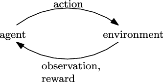
Figure 20. The classical RL training loop
The library has a wide variety of datasets ranging from classical control problems to complex 2D and 3D robotic manipulation tasks. It also exposes its registry and API as wrappers to adapt your custom environments, data, and models. This work relies on two such datasets—Atari 2600 games and a RET simulator developed by researchers at Ericsson as a gym wrapped environment.
4.3.1. Atari 2600 games
Atari 2600 games, which are implemented in the Arcade Learning Environment (Bellemare et al., Reference Bellemare, Naddaf, Veness and Bowling2013) are available on Gym. These problems are widely used for benchmarking the performance of RL algorithms (Hasselt, Reference Hasselt2010; Mnih et al., Reference Mnih, Badia, Balcan and Weinberger2016; Wang et al. Reference Wang, Schaul, Hessel, Hasselt, Lanctot and Freitas2016; Salimans et al., Reference Salimans2017; Conti et al., Reference Conti, Madhavan, Such, Lehman, Stanley and Clune2018). Each game consists of a range of actions, and game scores as rewards. The state of each game is the pixel data from an image. This is also known as a game frame. Figures 21 and 22 show examples from the game frames from four Atari 2600 games.
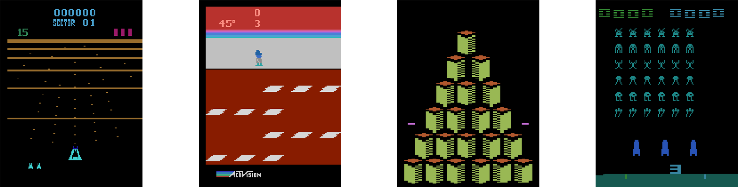
Figure 21. Game frames from 4 Atari 2600 games—beamrider, frostbite, qbert, spaceinvader
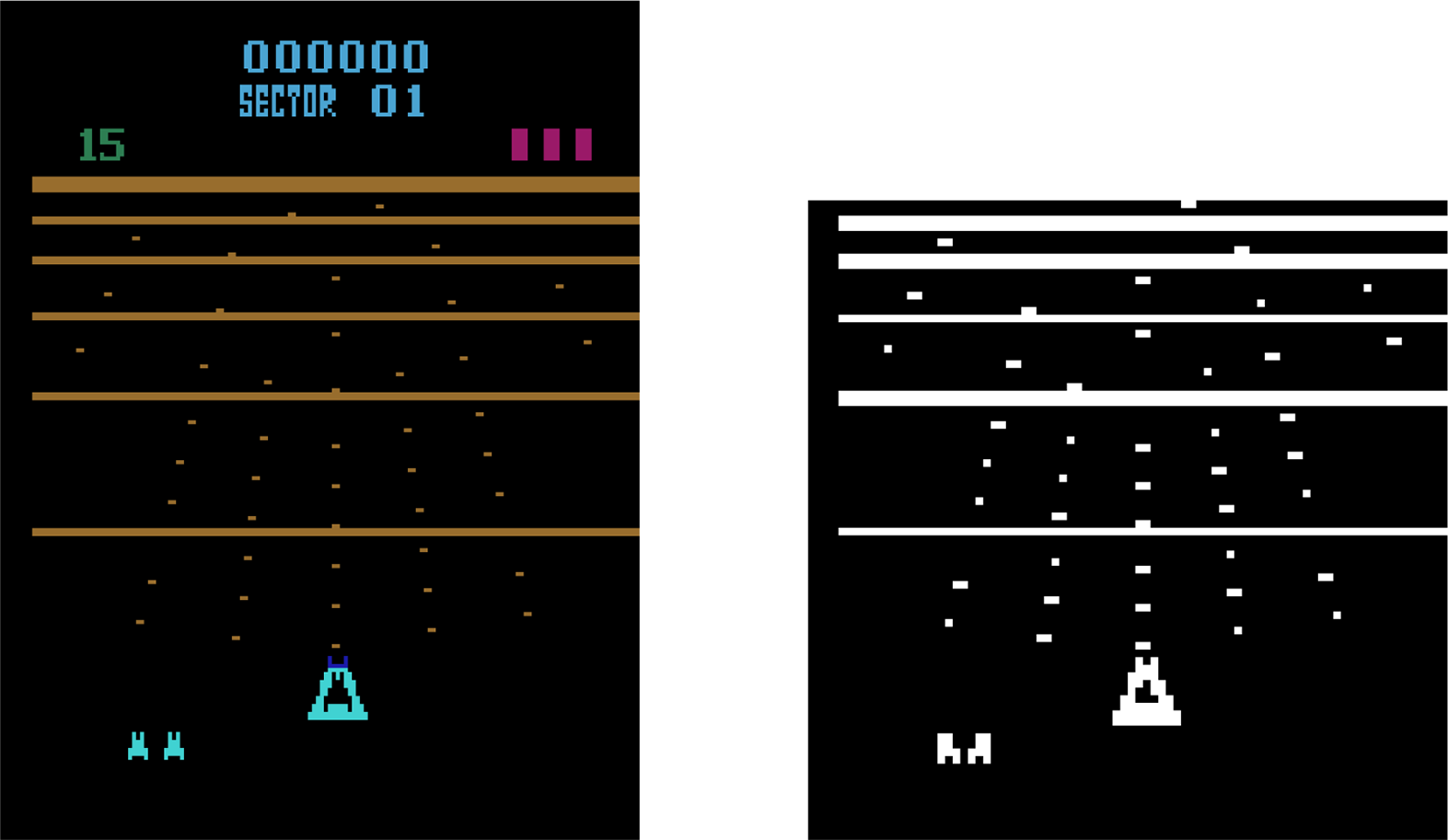
Figure 22. Original game frame (left) and preprocessed frame (right) using the first three steps
Gym has a collection of over 50 games. Each game is implemented as an environment in the library. The agent is provided with the current state and a list of possible actions. Once an action is selected by the agent, it is given a reward (positive or negative) by the model and the next state of the environment. The interaction is repeated until the environment returns a flag indicating the termination of the game. The technical specifications of all the games utilized in this work are available in Appendix A.1.
Data Preprocessing: Most games, have an image frame of size $210\times160\times3$
pixels which puts a heavy workload when training a NN, especially with several hidden layers. To reduce the dimensionality of inputs, some basic preprocessing steps are applied as suggested by researchers in the implementation of DQN (Mnih et al., Reference Mnih and Kavukcuoglu2015).
$210\times160\times3$
pixels which puts a heavy workload when training a NN, especially with several hidden layers. To reduce the dimensionality of inputs, some basic preprocessing steps are applied as suggested by researchers in the implementation of DQN (Mnih et al., Reference Mnih and Kavukcuoglu2015).
-
1. The game frame is first converted to a grayscale.
-
2. The grayscale image is down sampled to the size
$84\times84$
. -
3. The pixel values of the image are normalized between [0,1].
-
4. A training frame of size
$84\times84\times4$
is then produced by stacking 4 game frames together.


4.3.2. Remote electric tilt simulator by Ericsson
A use case of RL in telecommunications is RET optimization. For a better consumer experience and improved (), networks rely on making some adjustments to their configurations remotely. Antenna downtilt is the angle of inclination between the horizontal plan the radiating beam of the antenna which is shown in Figure 23. RET optimization is a technique to adjust the downtilt as mentioned above to improve certain Key Performance Indicators (KPIs) defined by the network. This framework is well suited for applying RL, and prior work using DQN has shown safe and reliable policies (Vannella et al., Reference Vannella2021).
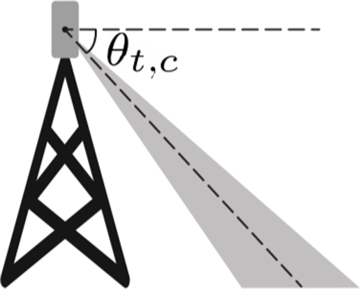
Figure 23. Antennae downtilt, $\theta_{t,c}$
for cell c at time t. Source Vannella et al. (Reference Vannella2021)
$\theta_{t,c}$
for cell c at time t. Source Vannella et al. (Reference Vannella2021)
The state of the environment comprises factors like congestion, overlapping, interference, overshooting and Reference Signal Receive Power (RSRP)Footnote 6. The actions include uptilt by 1 degree, downtilt by 1 degree and no tilt. After training, the simulated environment provides the overall improvement on four metrics, the Reward KPI, good traffic, bad traffic, and RRC congestionFootnote 7. The details about metrics are proprietary, however, a positive value for each metric is an indicator of a good policy.
4.4. Evaluation metrics
The metrics used for evaluating the results from the experiments are summarized below:
Speedup: In parallel processing, this notion was established by Amdahl’s argument (Amdahl, Reference Amdahl1967) as the ratio of the time taken by the best sequential algorithm (fastest) ( $T^*_{S}$
) to the time taken by a parallel algorithm (
$T^*_{S}$
) to the time taken by a parallel algorithm ( $T_{p}$
) for any computational problem. If the best sequential algorithm is not available or well defined, a common practice is to use the time taken by the parallel algorithm with 1 processor (
$T_{p}$
) for any computational problem. If the best sequential algorithm is not available or well defined, a common practice is to use the time taken by the parallel algorithm with 1 processor ( $T_{1}$
) as its surrogate.
$T_{1}$
) as its surrogate.
 \begin{equation}\begin{aligned} &S_{p}=\frac{T^*_{S}}{T_{p}} \approx \frac{T_{1}}{T_{p}} \quad \text{, p is the number of processors.} \end{aligned}\end{equation}
Linear speedup, also referred to as ideal speedup, is obtained when $S_{p}=p$
suggesting that the algorithm is perfectly scalable, which is infeasible to achieve in reality.
$S_{p}=p$
suggesting that the algorithm is perfectly scalable, which is infeasible to achieve in reality.
Efficiency: In parallel processing, it is the ratio of the speedup achieved by the parallel implementation of the algorithm, $S_p$
to the number of processors utilized, p.
$S_p$
to the number of processors utilized, p.
 \begin{equation} E=\frac{S_{p}}{p} = \frac{T^*_{S}}{pT_{p}} \approx \frac{T_{1}}{pT_{p}} \end{equation}
A typical value lies in the range of 0 and 1. Algorithms running on a single processor and parallel algorithms with a linear speedup have an efficiency of 1.
Cumulative reward: The goal of any RL policy is to optimize the expected return. Given a fixed time horizon of T, the objective is to find a sequential decision policy $\pi$
, that maximizes the expected return until the end of the time horizon. If we represent the sequence of rewards received after time t, by
$\pi$
, that maximizes the expected return until the end of the time horizon. If we represent the sequence of rewards received after time t, by $r_{t+1}, r_{t+2}, r_{t+3}, \ldots$
, then the cumulative reward is simply:
$r_{t+1}, r_{t+2}, r_{t+3}, \ldots$
, then the cumulative reward is simply:
 \begin{equation} G_{t} \doteq r_{t+1}+r_{t+2}+r_{t+3}+\cdots+r_{T} \end{equation}
Sample Efficiency: For any RL algorithm, sample efficiency is a measure of its efficiency in utilizing the experience gained by the agent, that is, the amount of experience on an average that an algorithm needs to generate in an environment in order to reach a certain level of performance. An algorithm can be termed sample efficient if it uses each sample from its experience optimally to generate a policy that achieves a high performance.
4.5. Experiments
Experiment 1: Comparison to gradient-based methods
In this experiment, the performance of Sp-GA is compared with two gradient-based RL methods, DQN (Mnih et al., Reference Mnih and Kavukcuoglu2015), a sequential algorithm and A3C (Mnih et al., Reference Mnih, Badia, Balcan and Weinberger2016), a distributed algorithm. The metrics used for evaluation are cumulative rewards and training time.
Table 2. Hyperparameters used to train Sp-GA on Atari 2600 games

Each algorithm was trained on 6 Atari 2600 games—beamrider, assault, spaceinvader, qbert, frostbite, and amidar for a maximum of 5 million training frames. The hyperparameters for DQN and A3C were obtained from the benchmarked results of rllib libraryFootnote 8 and for Sp-GA, they are mentioned in Table 2. The same architecture (Model 1) and preprocessing was utilized. The training started with a random number (maximum upto 30) of no-op action similar to prior work (Mnih et al., Reference Mnih and Kavukcuoglu2015). A single episode for DQN, A3C, and iteration for Sp-GA was capped at a maximum of 10K training frames.
Experiment 2: Comparison to gradient-free methods
In this experiment, the performance of Sp-GA is compared with two gradient-free techniques that also use EC-based methods for training, a simple GA (Conti et al., Reference Conti, Madhavan, Such, Lehman, Stanley and Clune2018), and ES (Salimans et al., Reference Salimans2017). The metrics used for evaluation are cumulative rewards.
Each algorithm was trained on 16 Atari 2600 games (list available in Appendix A.1) for a maximum of 25 million training frames. The hyperparameters for ES were obtained from the benchmarked results of rllib library. GA was implemented as a special case of Sp-GA without crossover and species-based initialization. All other parameters for GA and Sp-GA were kept the same which are mentioned in Table 2. The same architecture (Model 1) and preprocessing was utilized across algorithms. A single episode for ES and iteration for GA, Sp-GA was capped at a maximum of 10K training frames.
Experiment 3: Scalability Assessment of Sp-GA
In this experiment, the scalability of distributed Sp-GA is assessed by evaluating the speedup and efficiency. The efficacy of encoding is also tested by comparing memory utilization.
This experiment was conducted on a single Atari 2600 game—spaceinvader. Sp-GA was trained for a maximum of 500 000 training frames on clusters with different number of workers. A single iteration step was capped at a maximum of 1000 training frames. The population size was reduced to 100; all other hyperparameters were kept the same as mentioned in Table 2.
Experiment 4: Comparison of sample efficiency
In this experiment, the sample efficiency of Sp-GA, A3C, DQN, ES, and GA are compared. The algorithm that consistently obtains higher rewards with the increasing size of training frames is considered as more sample efficient. The results are computed on 3 Atari 2600 games chosen at random.
This experiment was conducted on 3 Atari 2600 games—frostbite, qbert and spaceinvader. The same training pipelines from Experiments 1 and 2 were used. The average rewards from all the algorithms were logged during training up to 5 million frames.
Experiment 5: Performance evaluation on RET optimization
The performance of Sp-GA is evaluated on the RET simulator provided by the host organization (Section 4.3.2) and compared to DQN. The evaluation metrics are provided by the simulator.
This experiment was conducted on RET simulator provided by the host organization. The implementation and hyperparameters for DQN were preconfigured and are mentioned in Appendix 3. Both algorithms were trained for a fixed number of iterations of 1500. The model architecture was kept the same (Model 2). The hyperparameters used by Sp-GA are summarized in Table 3
Table 3. Hyperparameters used to train Sp-GA on RET environment
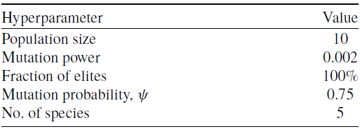
5. Results
Experiment 1 : Comparison to gradient-based methods
Table 4 summarizes the cumulative rewards achieved by Sp-GA, DQN, and A3C. Sp-GA trains a population of 200 neural networks, whereas DQN and A3C train a single neural network on the same amount of training frames. The cumulative reward of the elite model from Sp-GA is compared to the maximum episodic reward from the gradient-based methods for a fair comparison. Sp-GA outperforms DQN on all the games and A3C on 5 out of 6 games. The cumulative rewards on these benchmarks are not directly comparable to the results in Mnih et al. (Reference Mnih, Badia, Balcan and Weinberger2016), Salimans et al. (Reference Salimans2017), Conti et al. (Reference Conti, Madhavan, Such, Lehman, Stanley and Clune2018) due to training size being limited to 5M frames, but they support their findings that gradient-free methods can perform surprisingly well on RL tasks.
Table 4. Cumulative rewards achieved by DQN, A3C and Sp-GA on 6 Atari 2600 games
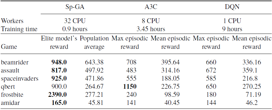
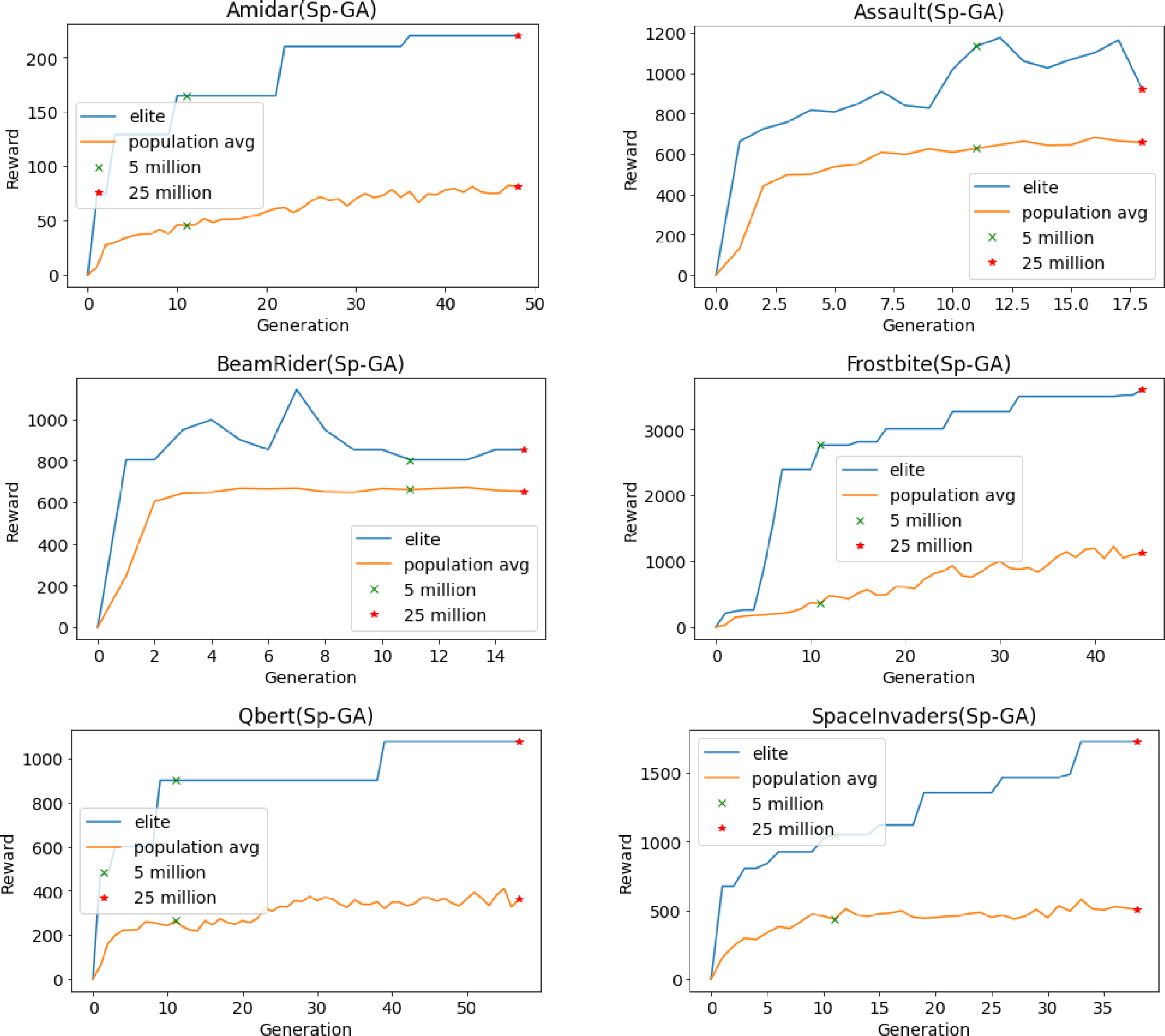
Figure 24. Elite model’s score and population average achieved by Sp-GA on Atari 2600 games for two milestones (5 million, 25 million training frames)

Figure 25. Maximum episodic reward for DQN, A3C on Atari 2600 games for 5 million training frames. The transparent lines represent the actual value, and the solid ones represent the smoothed values
Figure 25 shows the maximum episodic reward for DQN and A3C at each iteration for 5 million training frames. Figure 24 shows the elite model’s cumulative reward and the entire population’s average cumulative reward for each generation of Sp-GA. Two milestones have been highlighted in the figure—5 million training frames and 25 million training frames. With continued training, the performance of Sp-GA continues to improve in most of the games. The rate of improvement is lower for assault and beamrider, but it is still greater than DQN and A3C by a good margin. The decision of using the same hyperparameters across games might have contributed to this discrepancy. A fair comparison of all the algorithms in terms of training time is difficult due to the different number of CPUs utilized. However, the distributed Sp-GA, which is trained on a cluster of 32 CPUs is atleast 10 times faster than DQN and 4 times faster than A3C and trains 200 neural networks all at once.
These results corroborate the findings in Conti et al. (Reference Conti, Madhavan, Such, Lehman, Stanley and Clune2018) that EC-based methods like GAs can provide comparable performance to gradient-based algorithms while reducing the overall training time by a significant amount.
Experiment 2 : Comparison to gradient-free methods
Table 5 summarizes the cumulative rewards achieved by Sp-GA, a simple GA, and ES on 16 Atari 2600 games, each trained for about 25 Million training frames which are equivalent to 100 million game frames. The simple GA is a special case of Sp-GA with a single species and no crossover operator. Since the library implementation of ES only provides the average episodic reward, we compare them to the population’s average cumulative reward from Sp-GA and simple GA. The best performing algorithm for each game is highlighted in bold. Clearly, GA-based methods outperformed ES on 10 out of 16 games. Surprisingly, all of the algorithms scored a 0 on venture which is similar to the findings in Bellemare et al. (Reference Bellemare, Naddaf, Veness and Bowling2013). This specific game is known to require long-term planning. Our proposed algorithm and ES doesn’t involve a discount term when evaluation the cumulative reward which might have resulted in poor performance. Among GA-based methods, the elite models from Sp-GA outperformed simple GA on 9 out of 15 games (better model for each game is highlighted in green). The decision to use the same hyperparameters for all the games (and a single run being used) could have resulted in these results. The generational rewards for each game for all the algorithms are available in Appendix A.2. The library implementation of ES was twice as fast when compared to Sp-GA and simple GA which suggests some improvements might be needed in our implementation.
Table 5. Comparing the performance of Sp-GA with a simple genetic algorithm (GA) and evolution strategies (ES)
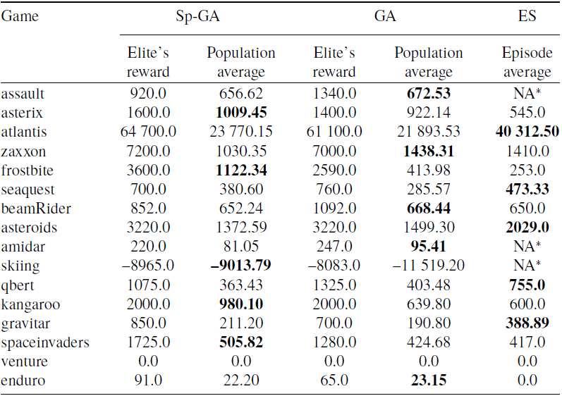
*Configuration for these Atari games are not implemented in the library.
This experiment demonstrates how different variants of GAs can be adapted to train neural networks for RL problems while still maintaining comparable performance to other gradient-free algorithms (Salimans et al., Reference Salimans2017; Conti et al., Reference Conti, Madhavan, Such, Lehman, Stanley and Clune2018).
Experiment 3 : Scalability assessment of Sp-GA
Figure 26 shows the average time per generation and total training time, which includes the time it took for communication among the workers, as a function of the number of processors. The total time, as well as the average generation time, is seen decreasing up to 32 CPUs. When the number of CPUs was increased to 40, the time taken rather increases. Possible reasons for this might be, the communication time between the workers posing a bottleneck, or congestion between the workers since these experiments are sent as jobs to clusters.
Figure 27 shows the parallel speedup of Sp-GA as a function of the number of CPUs. The speedup increases as the number of processors utilized are increased. Since the training time for 40 CPUs was higher than 32 CPUs, the speedup did not increase. Figure 28 shows the efficiency of the Sp-GA as a function of processors used. The algorithm is only optimal on a single CPU. With the increasing number of processors, the efficiency is decreasing which can be attributed to the additional communication time and CPUs remaining ideal post the fitness calculation.
Figure 18 shows the architecture of the model utilized for Experiments 1, 2, 3, and 4. Each neural network has a size of 6.73 MB. This becomes a significant memory and bandwidth bottleneck especially when the size of the population is increased. Table 6 shows the average size of an encoding of a neural network after training on 25M frames. The maximum size of an encoding which is $\sim$
600 bytes is still 10 000 folds less than the original size. This shows the efficiency of the encoding implemented for this work.
$\sim$
600 bytes is still 10 000 folds less than the original size. This shows the efficiency of the encoding implemented for this work.
Table 6. The number of generations, top elite’s species and average size of encoding after training Sp-GA for 25M frames
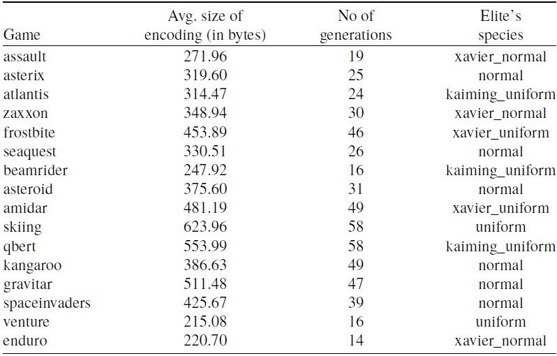
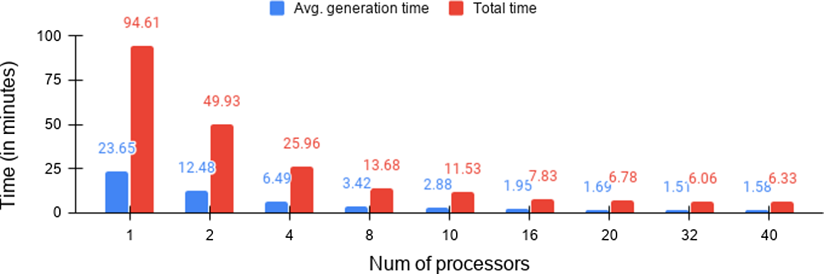
Figure 26. Total training time (including time for communication between workers) and average time per generation as a function of the number of CPU’s.
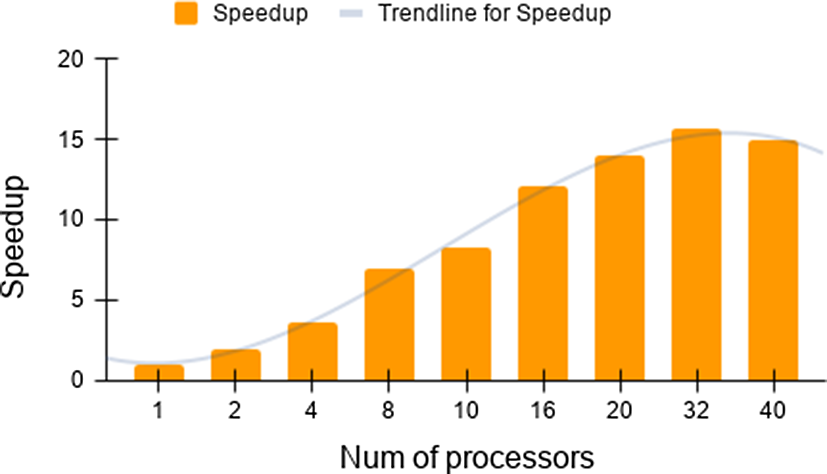
Figure 27. Parallel speedup as a function of number of processors
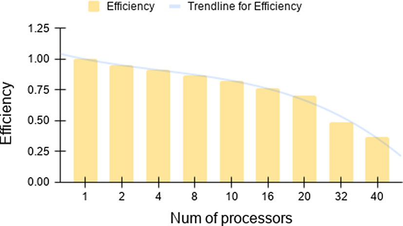
Figure 28. Efficiency as a function of number of processors
The results in this experiment demonstrate that GAs if implemented efficiently, are well suited for a distributed training framework that results in a reduction of overall training time.
Experiment 4 : Comparison of sample efficiency
Figure 29 compares the performance of Sp-GA, simple GA, DQN, A3C, and ES on 3 Atari 2600 games till 5M training frames which is equivalent to 20M games frames as experienced by the agent. For DQN, A3C and ES, the average episodic rewards (smoothed) and for Sp-GA and simple GA the population average rewards are reported for comparative analysis.
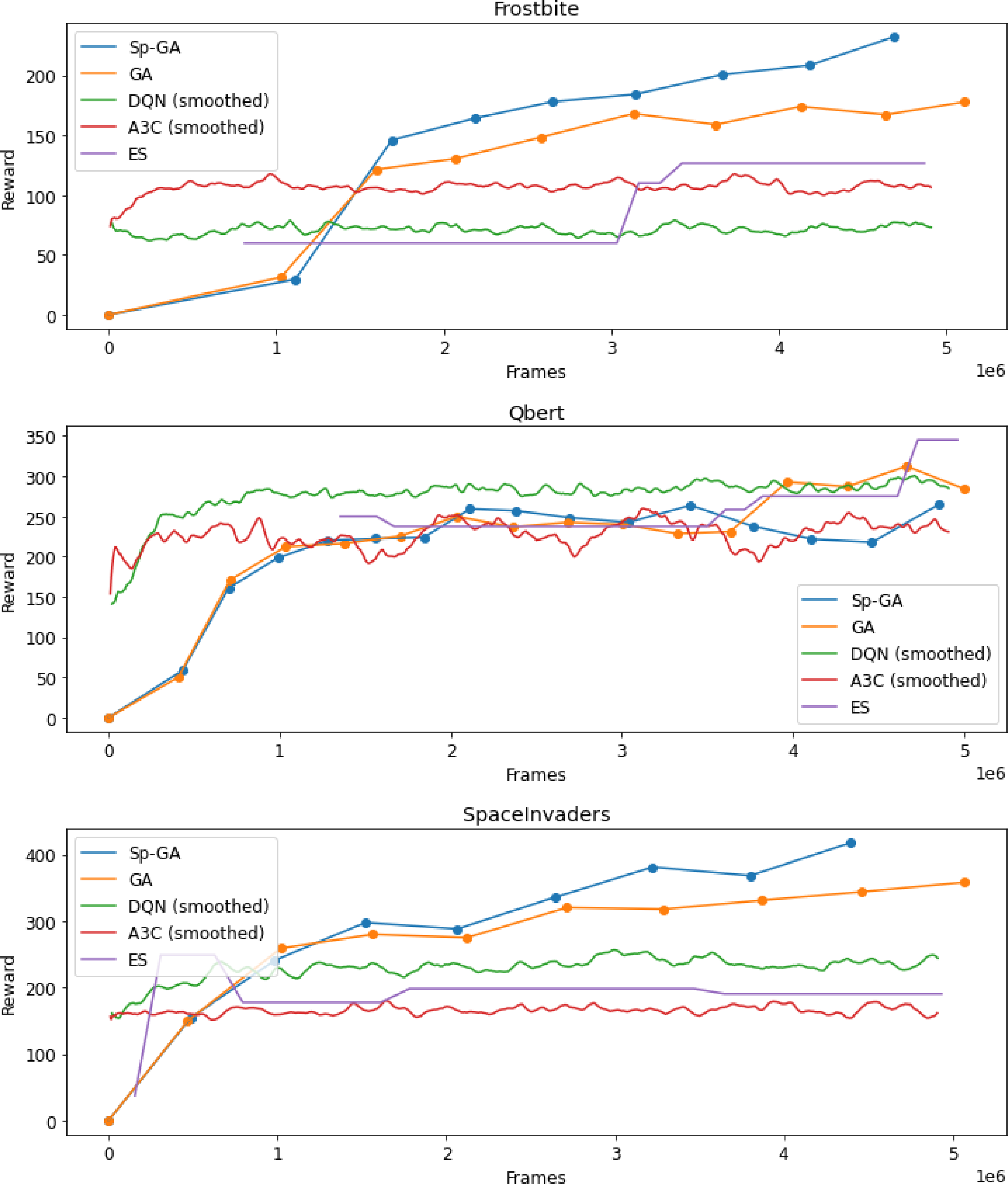
Figure 29. Comparison of sample efficiency on Atari 2600 games
For the games frostbite and spaceinvader, Sp-GA is relatively more sample efficient in comparison to other methods, especially after experiencing about 1.5M training frames. For a fixed sample size of 5M frames, Sp-GA outperform all other algorithms in 2 out 3 games. DQN proved to be the most efficient for qbert. It must be noted that a simple GA had impressive results and was a close second in all games. This strengthens the fact the gradient-free methods can be sample efficient in comparison to gradient-based methods in some situations.
These results suggest that EC-based methods can be sample efficient in comparison to gradient-based methods despite training multiple neural networks on the same amount of experience.
Experiment 5 : Performance evaluation on RET optimization
Figure 30 shows the reward for DQN and the elite model of Sp-GA at each iteration during training. This reward is a function of proprietary metrics. The performance of Sp-GA is better than DQN during the initial stages of the training, however, DQN seems to perform better later on. The results of this experiment were reported from a single run which might have resulted in a bias. In Sp-GA, each worker creates a copy of the environment it trains on; in this experiment, the memory requirements of the environment and the interaction time became a bottleneck. To compensate for it, the size of the population was reduced significantly, which might have resulted in a slight worse performance.
It is interesting to see that although DQN outperformed Sp-GA overall, there was a good improvement in all the metrics and KPIs of the environment. The experiment was conducted for a fixed amount of training steps, and not for a fixed duration of training time. It is possible that if Sp-GA was let to train for the same duration as DQN (which was significantly more), we would have seen better results. This can be investigated in future work.The results are reported in Table 7. The plots for all the metrics for both algorithms are available in Appendix A.1
Table 7. Average improvement of some KPI’s provided by the environment with respect to a set baseline. A positive value is an indicator of a good policy
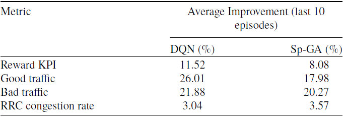
These results suggest that GAs are also effective when applied to RL problems in different domains, including complex optimization tasks in telecommunication.
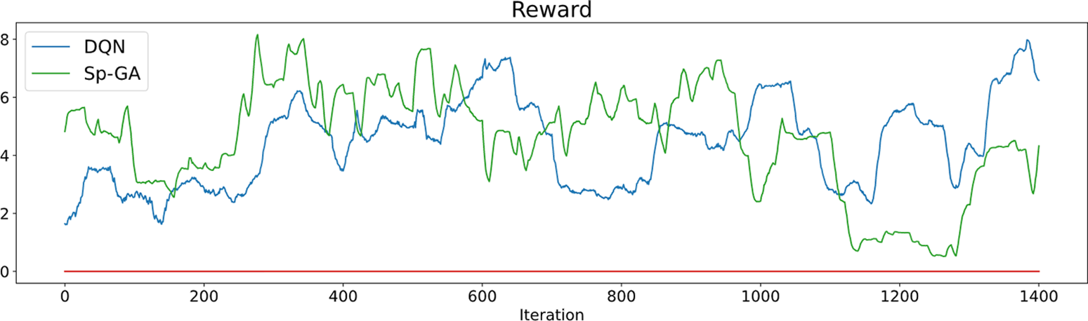
Figure 30. Reward KPI from the RET environment at each episode of training for DQN and Sp-GA. The red line highlights zero improvement
6. Discussion
The findings from this research outline the success of GAs and other Evolutionary Computation (EC)-based techniques as a scalable alternative to gradient-based algorithms for complex RL problems. Not only did Sp-GA outperform DQN and A3C on several established benchmarks, it also reduced the overall training time by a big margin. A big advantage of the proposed method is its ability to constantly explore and learn from its experience irrespective of the density of rewards.
The proposed model encoding proved to be highly efficient and yielded significant improvements in memory utilization and overall training time. The intuitive application of genetic operators in the encoding space did not hinder the parallel implementation of the algorithm. Sp-GA and simple GA even outperformed ES, another EC-based method, on multiple benchmarks.
The speedup of the parallel implementation increased consistently upto 32 CPUs. Increasing the number to 40 somehow resulted in worse performance. Apart from the communication time being a bottleneck, a possible explanation could be a bug in the libraries used in the implementation. The topology of the workers and the communication patterns play an important role in the efficiency of any parallel algorithm especially in ML (Neglia et al., Reference Neglia2019). The work relied on ray for the set up of clusters and communication and this might have been a limiting factor.
It is well known that RL algorithms are sample inefficient when compared to supervised techniques (Yu, Reference Yu2018), Sp-GA was sample efficient in a few cases, requiring fewer training samples to provide improved results. The successful implementation of Sp-GA for RET optimization and improvement in KPIs highlights that such gradient-free methods can also be applied to RL problems from other domains.
From these experiments, it can be concluded that repeated sampling around the region of good solutions can help discover better solutions without the need for estimating gradients. This hypothesis was also found out to be true by authors in Conti et al. (Reference Conti, Madhavan, Such, Lehman, Stanley and Clune2018), Salimans et al. (Reference Salimans2017). Although the results from our benchmarks are not directly comparable to the findings in Salimans et al. (Reference Salimans2017), Conti et al. (Reference Conti, Madhavan, Such, Lehman, Stanley and Clune2018), it was anticipated since the training was limited to only 25M frames on a subset of games due to computational constraints.
6.1. Opportunities for improvement
For a few benchmarks, the performance did not improve as much as the others. The could be attributed to the decision of using the same parameters for all the experiments. Tuning these parameters for each benchmark by doing a grid search should result in an improved performance.
There were a few situations where introducing random perturbations had unexpected effects, this was seen in the game venture where all of the gradient-free algorithms scored 0. In the experiments, a constant amount of mutation was applied to all the networks; it would be interesting to see what would happen if this mutation is annealed, similar to annealing of a learning rate. Another possible improvement could be adapting the mutation inversely to the fitness of a solution, that is, making small perturbations to good solutions, whereas big perturbations to low-scoring ones. Utilizing the same parameters across experiments seems to have limited the performance in the experiments.
An unexpected result from the experiments was a simple GA without crossover outperforming Sp-GA on a few benchmarks. Crossover, which is well-known strategy to improve the performance of GA (Holland, Reference Holland1992b) did not work as expected. A possible explanation for this might be its application in the space of encoding. Applying crossover, in such a way is a novel contribution which needs to investigated further as a part of future work.
7. Conclusions
In this work, we were successfully able to apply an evolutionary-based technique to train deep neural networks for several RL tasks from different domains. We have also demonstrated how different variants of GAs can be scaled and operators be applied in the encoding space.
The results from the experiments confirmed the findings from Salimans et al. (Reference Salimans2017), Conti et al. (Reference Conti, Madhavan, Such, Lehman, Stanley and Clune2018), that simple algorithms can perform surprisingly well on quite complex tasks. The final conclusions and insights to the research questions are summarized below:
-
1. EC-based RL algorithms like Sp-GA and simple GA can be applied to complex problems with a large state space. It is possible to outperform gradient-based as well gradient-free methods in terms of overall rewards and training time.
-
2. The scalability of the algorithm relies heavily on the efficacy of the model encoding. The proposed encoding worked pretty well which improved the parallel speedup and reduced the memory requirement significantly. A bottleneck, when the communication time between workers shadowed the evaluation time was observed when a large number of processors were utilized.
-
3. The improvements in sample efficiency were not significant and requires further investigation. A fair comparison of all the algorithms is difficult since the training procedures are inherently different. Gradient-based methods train a single NN where as population-based methods train multiple NN on the same amount of experience. Each NN from the population only gets to train on a fraction of the experience. Surprisingly, even with this issue, Sp-GA improves sample efficiency in a few benchmarks.
-
4. The algorithm is also successful in other domains. It must be noted, EC-based methods work on copies of environments in parallel. If these environments are very big, the algorithm cannot be scaled to its true potential. The concept of shared environments can be investigated to overcome this issue.
8. Future work
Future efforts will be devoted toward an investigative study on the effect of genetic operators in the encoding space. Our work was limited to Gaussian operator for mutation and single-point crossover. A plethora of strategies that improve the performance of GAs are available (Holland, Reference Holland1992a) which can directly be applied to Sp-GA. Also, the training can be extended to the complete set of Atari 2600 benchmarks on 1B training frames for benchmarking the results against (Salimans et al., Reference Salimans2017; Conti et al., Reference Conti, Madhavan, Such, Lehman, Stanley and Clune2018).
The performance of Deep Neural Networks (DNNs) can be improved by utilizing techniques like dropout (Srivastava et al., Reference Srivastava2014), LSTM and GRU (Hochreiter & Schmidhuber, Reference Hochreiter and Schmidhuber1997; Cho et al., Reference Cho2014), residual networks (He et al., Reference He2015a), and scheduled annealing of parameters (Robbins & Monro, Reference Robbins and Monro1951). Such techniques can also be applied to the proposed algorithm. Lastly, a hybrid approach combing both evolutionary and MDP-based methods can be investigated.
APPENDIX A Supplementary Information
Appendix A. Additional Technical Information
This section contains some additional technical information about the work. Table A.1 contains the technical specifications of the Atari 2600 games utilized in the work. Table A.2 provides the hyperparameter used for training DQN on RET simulator. Table A.3 gives the technical details of Experiment 4.
Table A.1. Specification of Atari 2600 games used for the experiments
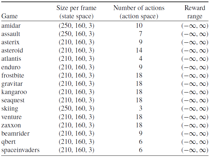
Table A.2. Hyperparameters used to train DQN on RET environment
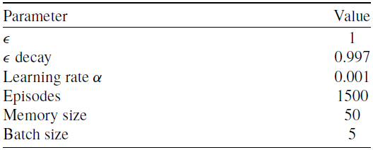
Table A.3. Total training time (including communication between workers) and average time taken per generation as a function of number of CPU’s
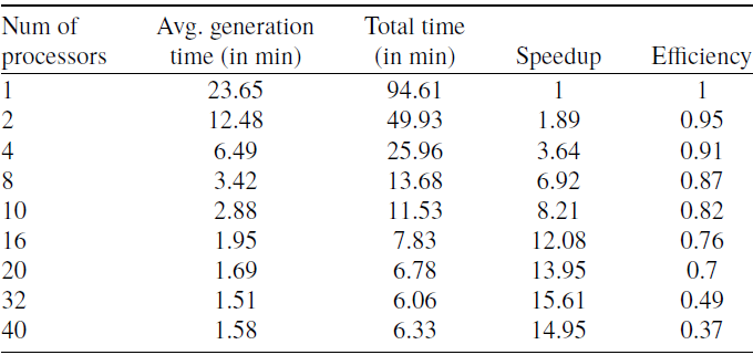
Appendix A. Additional Results
This section presents some additional results from the experiments.
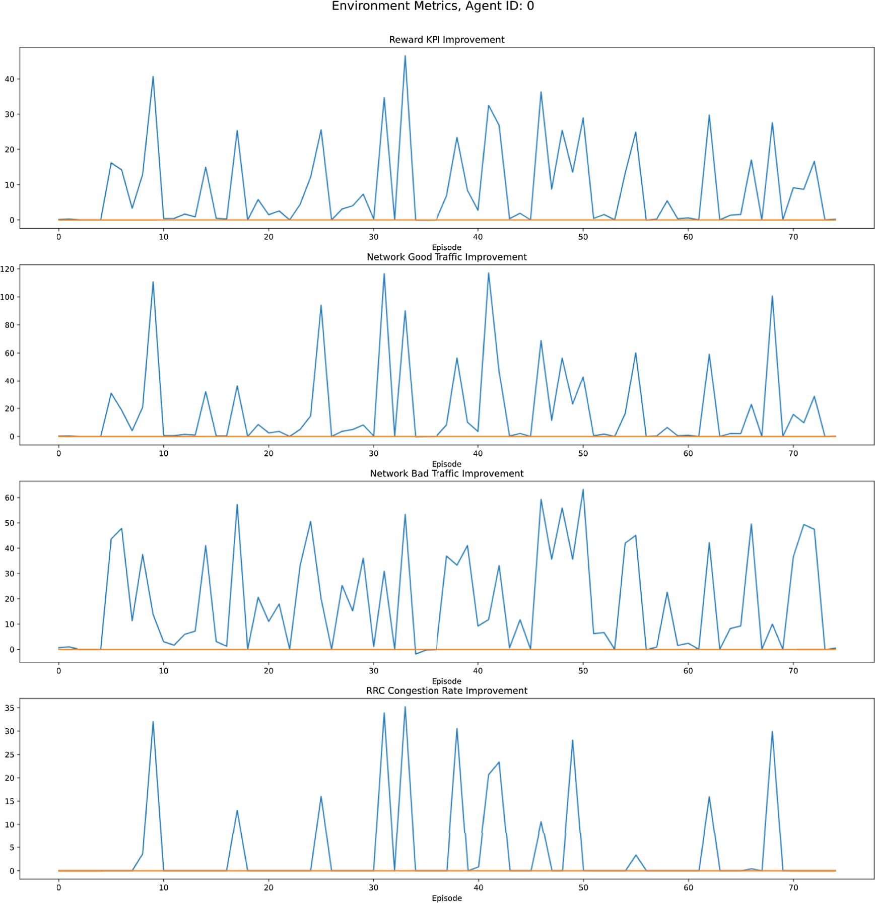
Figure A.1. Metrics returned by RET environment at each episode during training for Sp-GA
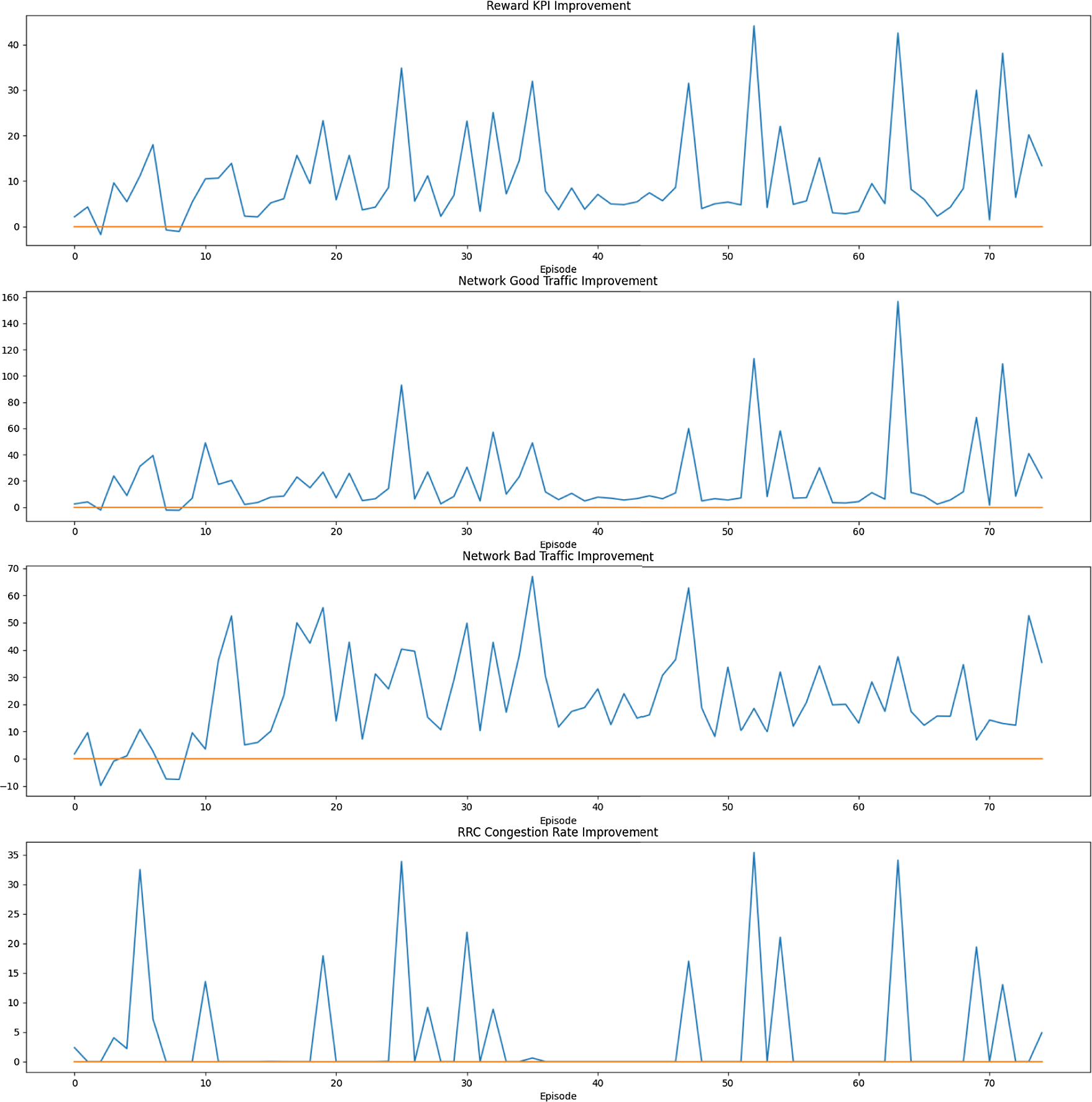
Figure A.2. Metrics returned by RET environment at each episode during training for DQN
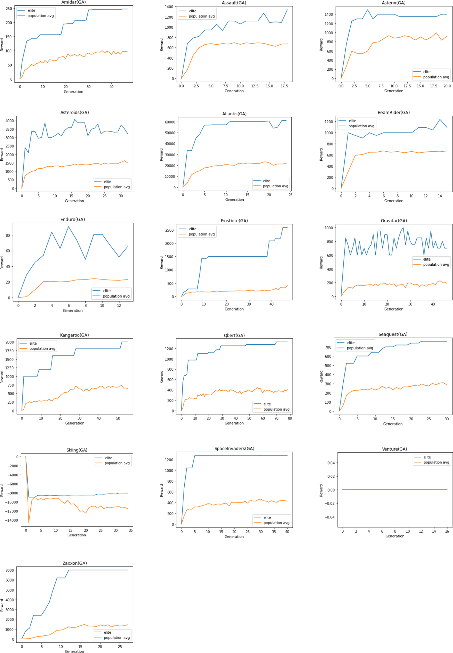
Figure A.3. Elite model’s score and population average achieved by GA on Atari 2600 games
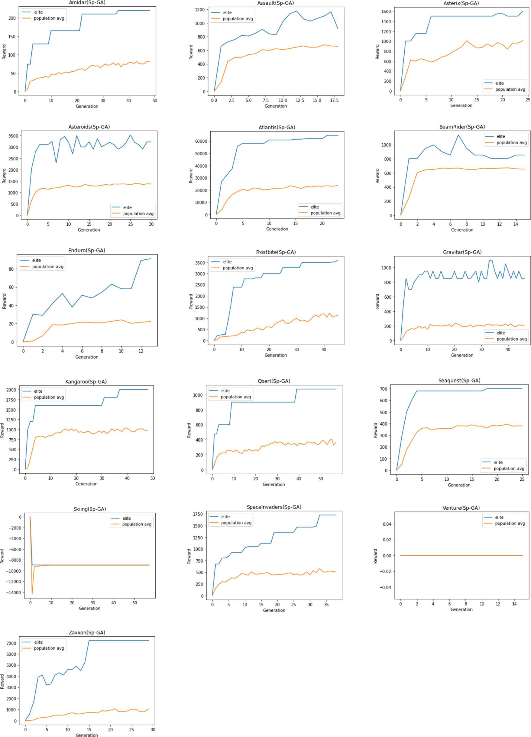
Figure A.4. Elite model’s score and population average achieved by Sp-GA on Atari 2600 games

Figure A.5. Average episodic reward achieved by ES on Atari 2600 games

Figure A.6. Maximum and average episodic reward achieved by DQN on Atari 2600 games
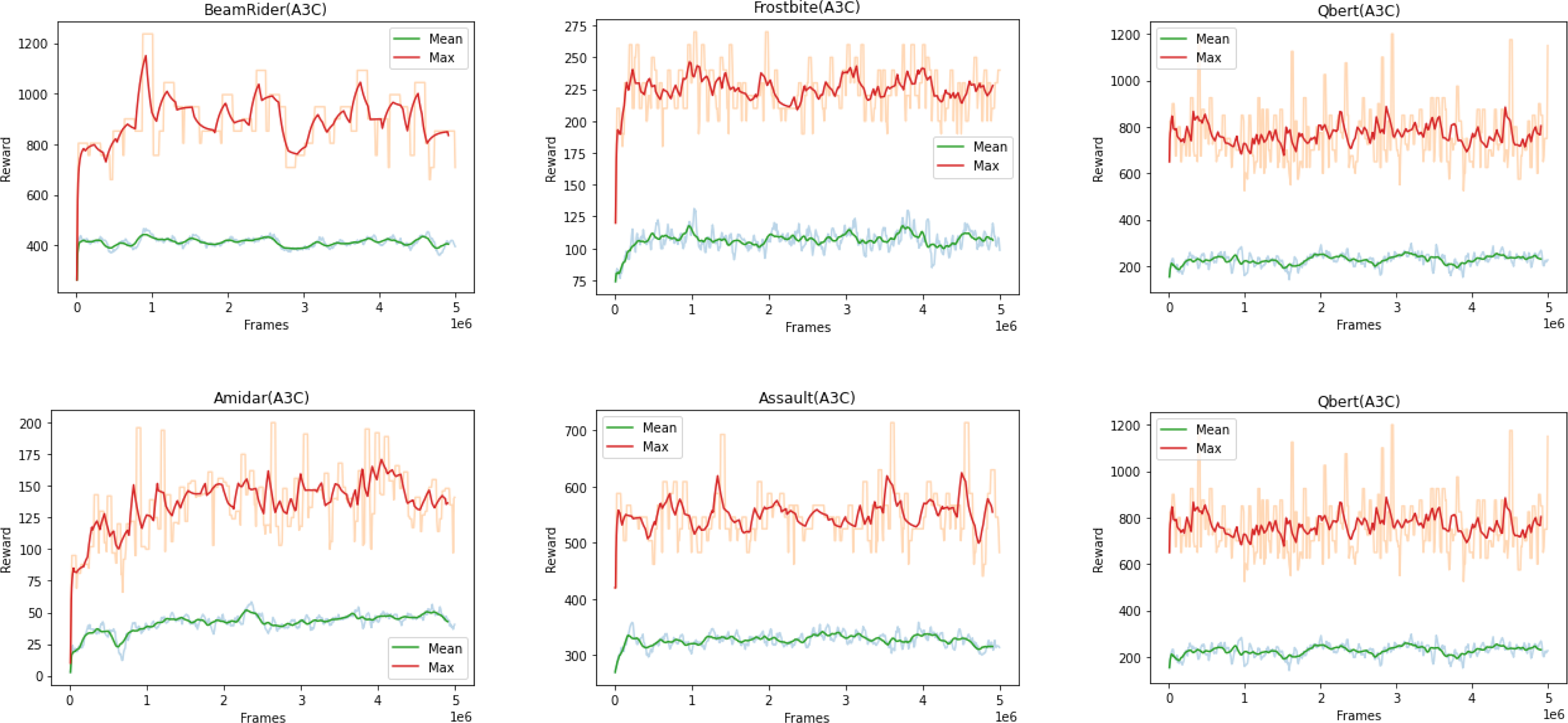
Figure A.7. Maximum and average episodic reward achieved by A3C on Atari 2600 games


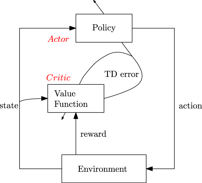


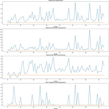


 Open access