


1 Introduction
To a continuous, surjective self-map
 $f$
of a compact metric space one can associate its topological entropy. Roughly speaking, this number measures how fast general points spread out under the iterations of the automorphism. By the work of Gromov [Reference Gromov6] and Yomdin [Reference Yomdin18], on a compact Kähler manifold
$f$
of a compact metric space one can associate its topological entropy. Roughly speaking, this number measures how fast general points spread out under the iterations of the automorphism. By the work of Gromov [Reference Gromov6] and Yomdin [Reference Yomdin18], on a compact Kähler manifold
 $X$
, the topological entropy can be calculated in terms of the action of
$X$
, the topological entropy can be calculated in terms of the action of
 $f$
on the cohomology groups
$f$
on the cohomology groups
 $H^{\ast }(X,\mathbb{Z})$
. In this case, the topological entropy is either zero or the logarithm of an algebraic number. More precisely, for K3 surfaces it is a Salem number. The degree of its minimal polynomial over
$H^{\ast }(X,\mathbb{Z})$
. In this case, the topological entropy is either zero or the logarithm of an algebraic number. More precisely, for K3 surfaces it is a Salem number. The degree of its minimal polynomial over
 $\mathbb{Q}$
is called its Salem degree. Esnault and Srinivas [Reference Esnault and Srinivas5] extended the notion of entropy to projective surfaces over an algebraically closed field of arbitrary characteristic.
$\mathbb{Q}$
is called its Salem degree. Esnault and Srinivas [Reference Esnault and Srinivas5] extended the notion of entropy to projective surfaces over an algebraically closed field of arbitrary characteristic.
Salem numbers of degree 22 were used by McMullen [Reference McMullen9] to construct K3 surfaces admitting an automorphism with Siegel disks. These are domains on which
 $f$
acts by an irrational rotation. Since the Salem degree of a projective surface is bounded by its Picard number
$f$
acts by an irrational rotation. Since the Salem degree of a projective surface is bounded by its Picard number
 $\unicode[STIX]{x1D70C}\leqslant 20$
, McMullen’s examples cannot be projective. They remain abstract objects.
$\unicode[STIX]{x1D70C}\leqslant 20$
, McMullen’s examples cannot be projective. They remain abstract objects.
However, in positive characteristic, there exist K3 surfaces with Picard number 22, so there may exist automorphisms of Salem degree 22. As pointed out by Esnault and Oguiso [Reference Esnault and Oguiso3], a specific feature of such automorphisms is that they do not lift to any characteristic zero model. One such surface is the supersingular K3 surface
 $X(p)$
of Artin invariant one defined over
$X(p)$
of Artin invariant one defined over
 $\overline{\mathbb{F}}_{p}$
. Abstractly, Blanc and Cantat [Reference Blanc and Cantat2] and Esnault et al. [Reference Esnault, Oguiso and Yu4] proved the existence of automorphisms of Salem degree 22 on
$\overline{\mathbb{F}}_{p}$
. Abstractly, Blanc and Cantat [Reference Blanc and Cantat2] and Esnault et al. [Reference Esnault, Oguiso and Yu4] proved the existence of automorphisms of Salem degree 22 on
 $X(p)$
for
$X(p)$
for
 $p\neq 5$
, 7, 13, while Shimada [Reference Shimada15] exhibited such automorphisms on every supersingular K3 surface in all odd characteristics
$p\neq 5$
, 7, 13, while Shimada [Reference Shimada15] exhibited such automorphisms on every supersingular K3 surface in all odd characteristics
 $p\leqslant 7919$
using double plane involutions. Meanwhile, Schütt [Reference Schütt12] exhibited explicit automorphisms of Salem degree 22 on
$p\leqslant 7919$
using double plane involutions. Meanwhile, Schütt [Reference Schütt12] exhibited explicit automorphisms of Salem degree 22 on
 $X(p)$
for all
$X(p)$
for all
 $p\equiv 2~\text{mod}\,3$
using elliptic fibrations.
$p\equiv 2~\text{mod}\,3$
using elliptic fibrations.
Building on his methods, we obtain the main result of this paper.
Theorem 1.1. The supersingular K3 surface
 $X(p)$
of Artin invariant one admits explicit automorphisms of Salem degree 22 for all primes
$X(p)$
of Artin invariant one admits explicit automorphisms of Salem degree 22 for all primes
 $p\equiv 3~\text{mod}\,4$
. Such automorphisms do not lift to any characteristic zero model of
$p\equiv 3~\text{mod}\,4$
. Such automorphisms do not lift to any characteristic zero model of
 $X(p)$
.
$X(p)$
.
Let
 $X$
be the K3 surface over
$X$
be the K3 surface over
 $\mathbb{Q}$
defined by
$\mathbb{Q}$
defined by
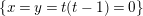
 $y^{2}=x^{3}+t^{3}(t-1)^{2}x$
. For
$y^{2}=x^{3}+t^{3}(t-1)^{2}x$
. For
 $p\equiv 3~\text{mod}\,4$
, its specialization mod
$p\equiv 3~\text{mod}\,4$
, its specialization mod
 $p$
is the supersingular K3 surface
$p$
is the supersingular K3 surface
 $X(p)$
of Artin invariant one. The automorphisms are constructed in the following steps.
$X(p)$
of Artin invariant one. The automorphisms are constructed in the following steps.
-
(1) Find generators of
 $NS(X)$
using the elliptic fibration.
$NS(X)$
using the elliptic fibration. -
(2) Complement the generators of
$NS(X)$
by two sections
$P,R$
to generators of
$NS(X(p))$
using a purely inseparable base change. -
(3) Compute the intersection matrix of
$NS(X(p))$
. -
(4) Search for extended
$ADE$
-configurations of
$(-2)$
-curves in
$NS(X)$
. These induce elliptic fibrations on
$X$
. -
(5)
$P$
and
$R$
induce sections of the new elliptic fibration. -
(6) The sections induce automorphisms of
$X(p)$
. Compute their action on
$NS(X(p))$
. -
(7) Compose automorphisms obtained from different fibrations to obtain one of the desired Salem degree.


2 Supersingular K3 surfaces
A K3 surface over an algebraically closed field
 $k=\overline{k}$
is a smooth surface with
$k=\overline{k}$
is a smooth surface with
 $$\begin{eqnarray}h^{1}(X,{\mathcal{O}}_{X})=0,\quad \unicode[STIX]{x1D714}_{X}\cong {\mathcal{O}}_{X}.\end{eqnarray}$$
Common examples are smooth quartics in
 $\mathbb{P}^{3}$
and double covers of
$\mathbb{P}^{3}$
and double covers of
 $\mathbb{P}^{2}$
branched over a smooth sextic. The group of divisors modulo algebraic equivalence is called the Néron–Severi group
$\mathbb{P}^{2}$
branched over a smooth sextic. The group of divisors modulo algebraic equivalence is called the Néron–Severi group
 $NS(X)$
. Its rank is called the Picard number. Equipped with the intersection pairing,
$NS(X)$
. Its rank is called the Picard number. Equipped with the intersection pairing,
 $NS(X)$
is a lattice (see Section 4). A singular K3 surface over
$NS(X)$
is a lattice (see Section 4). A singular K3 surface over
 $\mathbb{C}$
is one whose Picard number
$\mathbb{C}$
is one whose Picard number
 $$\begin{eqnarray}\unicode[STIX]{x1D70C}(X)=20=h^{1,1}(X),\end{eqnarray}$$
which is the maximal possible. Here “singular” is meant in the sense of exceptional rather than nonsmooth. In positive characteristic, however, the Picard number is only bounded by the second Betti number
 $b_{2}(X)=22$
, and K3 surfaces reaching the maximum possible Picard number
$b_{2}(X)=22$
, and K3 surfaces reaching the maximum possible Picard number
 $$\begin{eqnarray}\unicode[STIX]{x1D70C}(X)=22=b_{2}(X)\end{eqnarray}$$
are called supersingular. Supersingular K3 surfaces are classified according to their Artin invariant
 $\unicode[STIX]{x1D70E}$
defined by
$\unicode[STIX]{x1D70E}$
defined by
 $\det NS(X)=-p^{2\unicode[STIX]{x1D70E}},\unicode[STIX]{x1D70E}\in \{1,\ldots ,10\}$
(see [Reference Artin1]). By the work of Ogus [Reference Ogus10], there is a unique K3 surface of Artin invariant
$\det NS(X)=-p^{2\unicode[STIX]{x1D70E}},\unicode[STIX]{x1D70E}\in \{1,\ldots ,10\}$
(see [Reference Artin1]). By the work of Ogus [Reference Ogus10], there is a unique K3 surface of Artin invariant
 $\unicode[STIX]{x1D70E}=1$
, over
$\unicode[STIX]{x1D70E}=1$
, over
 $k=\overline{k}$
of characteristic
$k=\overline{k}$
of characteristic
 $p$
. We denote it by
$p$
. We denote it by
 $X(p)$
.
$X(p)$
.
Supersingular K3 surfaces arise from singular K3 surfaces as follows.
Proposition 2.1. [Reference Schütt12]
Let
 $X$
be a singular K3 surface defined over a number field
$X$
be a singular K3 surface defined over a number field
 $L$
, and let
$L$
, and let
 $d=\det NS(X)$
. If
$d=\det NS(X)$
. If
 $\mathfrak{p}$
is a prime of good reduction above
$\mathfrak{p}$
is a prime of good reduction above
 $p\in \mathbb{N}$
, then
$p\in \mathbb{N}$
, then
 $X_{p}:=X\times \text{Spec}\,\overline{\mathbb{F}}_{p}$
is supersingular if
$X_{p}:=X\times \text{Spec}\,\overline{\mathbb{F}}_{p}$
is supersingular if
 $p$
is inert in
$p$
is inert in
 $\mathbb{Q}(\sqrt{d})$
.
$\mathbb{Q}(\sqrt{d})$
.
As noticed by Shimada [Reference Shimada14], if
 $\det NS(X)$
is coprime to
$\det NS(X)$
is coprime to
 $p$
, then the Artin invariant is
$p$
, then the Artin invariant is
 $\unicode[STIX]{x1D70E}=1$
. The reason for this is that
$\unicode[STIX]{x1D70E}=1$
. The reason for this is that
 $NS(X){\hookrightarrow}NS(X_{p})$
implies
$NS(X){\hookrightarrow}NS(X_{p})$
implies
 $\unicode[STIX]{x1D70E}=1$
.
$\unicode[STIX]{x1D70E}=1$
.
3 Automorphisms and dynamics
A Salem polynomial is an irreducible monic polynomial
 $S(x)\in \mathbb{Z}[x]$
of degree
$S(x)\in \mathbb{Z}[x]$
of degree
 $2d$
such that its complex roots are of the form
$2d$
such that its complex roots are of the form
 $$\begin{eqnarray}a>1,\qquad a^{-1}<1,\qquad \unicode[STIX]{x1D6FC}_{i},\overline{\unicode[STIX]{x1D6FC}}_{i}\in S^{1},\quad i\in \{1,\ldots ,d-1\}.\end{eqnarray}$$
The unique positive root
 $a$
outside the unit disk is called a Salem number.
$a$
outside the unit disk is called a Salem number.
The following theorem is due to McMullen [Reference McMullen9] over
 $\mathbb{C}$
and Esnault and Srinivas [Reference Esnault and Srinivas5] in positive characteristic.
$\mathbb{C}$
and Esnault and Srinivas [Reference Esnault and Srinivas5] in positive characteristic.
Theorem 3.1. Let
 $X$
be a smooth projective K3 surface over an algebraically closed field
$X$
be a smooth projective K3 surface over an algebraically closed field
 $k=\overline{k}$
, and let
$k=\overline{k}$
, and let
 $f\in \mathit{Aut}(X)$
be an automorphism. Then, the characteristic polynomial of
$f\in \mathit{Aut}(X)$
be an automorphism. Then, the characteristic polynomial of
 $f^{\ast }|H_{\acute{e} t}^{2}(X,\mathbb{Q}_{l}(1))$
(char
$f^{\ast }|H_{\acute{e} t}^{2}(X,\mathbb{Q}_{l}(1))$
(char
 $k\neq l$
) factors into cyclotomic polynomials and at most one Salem polynomial. If a Salem factor
$k\neq l$
) factors into cyclotomic polynomials and at most one Salem polynomial. If a Salem factor
 $S(x)$
occurs, then
$S(x)$
occurs, then
 $\ker S(f^{\ast })\subseteq NS(X)$
.
$\ker S(f^{\ast })\subseteq NS(X)$
.
Notice that over
 $\mathbb{C}$
we can work equally well with the singular cohomology groups
$\mathbb{C}$
we can work equally well with the singular cohomology groups
 $H^{2}(X,\mathbb{Z})$
and prove the result via Hodge decomposition. The theorem motivates the following definition. Given a smooth projective surface over an algebraically closed field and an automorphism
$H^{2}(X,\mathbb{Z})$
and prove the result via Hodge decomposition. The theorem motivates the following definition. Given a smooth projective surface over an algebraically closed field and an automorphism
 $f:X\rightarrow X$
, the entropy
$f:X\rightarrow X$
, the entropy
 $h(f)$
of
$h(f)$
of
 $f$
is defined as
$f$
is defined as
 $$\begin{eqnarray}h(f):=\log r(f^{\ast }|NS(X)),\end{eqnarray}$$
where
 $r(f^{\ast }|NS(X))$
is the spectral radius of the linear map
$r(f^{\ast }|NS(X))$
is the spectral radius of the linear map
 $f^{\ast }|NS(X)\otimes \mathbb{Q}$
; that is, the maximum of the absolute values of its complex eigenvalues. The entropy is either zero or the logarithm of a Salem number
$f^{\ast }|NS(X)\otimes \mathbb{Q}$
; that is, the maximum of the absolute values of its complex eigenvalues. The entropy is either zero or the logarithm of a Salem number
 $a$
. The degree of the Salem polynomial corresponding to
$a$
. The degree of the Salem polynomial corresponding to
 $a$
is called the Salem degree of
$a$
is called the Salem degree of
 $f$
.
$f$
.
By the work of Esnault and Srinivas [Reference Esnault and Srinivas5], this is compatible with the definition of topological entropy for smooth complex projective surfaces.
Over
 $\mathbb{C}$
, due to Hodge theory, the rank of the Néron–Severi group is bounded by
$\mathbb{C}$
, due to Hodge theory, the rank of the Néron–Severi group is bounded by
 $20=h^{1,1}(X)$
. Hence, an automorphism on a complex projective K3 surface has Salem degree at most 20. In the nonprojective case, McMullen [Reference McMullen9] constructed K3 surfaces with automorphisms of Salem degree 22. In positive characteristic, however, K3 surfaces may have Picard rank 22, and there automorphisms of Salem degree 22 occur. A specific feature of such automorphisms is that they do not lift to any characteristic zero model.
$20=h^{1,1}(X)$
. Hence, an automorphism on a complex projective K3 surface has Salem degree at most 20. In the nonprojective case, McMullen [Reference McMullen9] constructed K3 surfaces with automorphisms of Salem degree 22. In positive characteristic, however, K3 surfaces may have Picard rank 22, and there automorphisms of Salem degree 22 occur. A specific feature of such automorphisms is that they do not lift to any characteristic zero model.
4 Lattices
In this section, we fix our notation concerning lattices. A lattice
 $L$
is a finitely generated free
$L$
is a finitely generated free
 $\mathbb{Z}$
module equipped with a nondegenerate symmetric bilinear pairing
$\mathbb{Z}$
module equipped with a nondegenerate symmetric bilinear pairing
 $L\times L\rightarrow \mathbb{Q}$
. If it is integer valued, then the lattice is called integral. The pairing identifies
$L\times L\rightarrow \mathbb{Q}$
. If it is integer valued, then the lattice is called integral. The pairing identifies
 $$\begin{eqnarray}\text{Hom}(L,\mathbb{Z})\cong L^{\ast }:=\{x\in L\otimes \mathbb{Q}|x.L\subseteq \mathbb{Z}\}.\end{eqnarray}$$
If
 $L$
is integral, it induces an embedding
$L$
is integral, it induces an embedding
 $L{\hookrightarrow}L^{\ast }$
. The finite quotient
$L{\hookrightarrow}L^{\ast }$
. The finite quotient
 $A_{L}:=L^{\ast }/L$
is called the discriminant group of
$A_{L}:=L^{\ast }/L$
is called the discriminant group of
 $L$
. Given a
$L$
. Given a
 $\mathbb{Z}$
-basis
$\mathbb{Z}$
-basis
 $(b_{i})$
, the determinant of the Gram matrix
$(b_{i})$
, the determinant of the Gram matrix
 $(b_{i}.b_{j})_{ij}$
is independent of the choice of basis and is called the determinant of
$(b_{i}.b_{j})_{ij}$
is independent of the choice of basis and is called the determinant of
 $L$
. Its absolute value is the order of the discriminant group. In this basis, the dual lattice is generated by the columns of
$L$
. Its absolute value is the order of the discriminant group. In this basis, the dual lattice is generated by the columns of
 $(b_{ij})^{-1}$
. Given an embedding
$(b_{ij})^{-1}$
. Given an embedding
 $M{\hookrightarrow}L$
of integral lattices of the same rank,
$M{\hookrightarrow}L$
of integral lattices of the same rank,
 $A_{L}$
is a subquotient of
$A_{L}$
is a subquotient of
 $A_{M}$
and we get
$A_{M}$
and we get
 $$\begin{eqnarray}\det M=[L:M]^{2}\det L.\end{eqnarray}$$
A lattice is called unimodular if it is integral and has
 $|\text{det}\,L|=1$
. An embedding
$|\text{det}\,L|=1$
. An embedding
 $M{\hookrightarrow}L$
of lattices is called primitive if
$M{\hookrightarrow}L$
of lattices is called primitive if
 $L/M:=L/im(M)$
is torsion free. If
$L/M:=L/im(M)$
is torsion free. If
 $M{\hookrightarrow}L$
is a primitive embedding of integral lattices and
$M{\hookrightarrow}L$
is a primitive embedding of integral lattices and
 $L$
is unimodular, then
$L$
is unimodular, then
 $A_{M}\cong A_{M^{\bot }}$
, where
$A_{M}\cong A_{M^{\bot }}$
, where
 $M^{\bot }$
is the orthogonal complement of
$M^{\bot }$
is the orthogonal complement of
 $M$
in
$M$
in
 $L$
. We define the length of a finite abelian group by its minimum number of generators. Note that
$L$
. We define the length of a finite abelian group by its minimum number of generators. Note that
 $l(A_{L})\leqslant \text{rk}\,L$
. A lattice is called
$l(A_{L})\leqslant \text{rk}\,L$
. A lattice is called
 $p$
-elementary if
$p$
-elementary if
 $pA_{L}=0$
, or equivalently if
$pA_{L}=0$
, or equivalently if
 $A_{L}$
is an
$A_{L}$
is an
 $\mathbb{F}_{p}$
vector space.
$\mathbb{F}_{p}$
vector space.
5 Elliptic fibrations on K3 surfaces
A genus-one fibration on a surface
 $X$
is a surjective map
$X$
is a surjective map
 $$\begin{eqnarray}\unicode[STIX]{x1D70B}:X\rightarrow C\end{eqnarray}$$
to a smooth curve
 $C$
such that the generic fiber is a smooth curve of genus one. We call it an elliptic fibration, if the additional datum of a section
$C$
such that the generic fiber is a smooth curve of genus one. We call it an elliptic fibration, if the additional datum of a section
 $O$
of
$O$
of
 $\unicode[STIX]{x1D70B}$
is given. Indeed, all genus-one fibrations occurring throughout this paper admit a section. This turns the generic fiber of an elliptic fibration into an elliptic curve
$\unicode[STIX]{x1D70B}$
is given. Indeed, all genus-one fibrations occurring throughout this paper admit a section. This turns the generic fiber of an elliptic fibration into an elliptic curve
 $E$
over
$E$
over
 $K=k(C)$
, the function field of
$K=k(C)$
, the function field of
 $C$
. For a K3 surface,
$C$
. For a K3 surface,
 $C=\mathbb{P}^{1}$
is the only possibility. There is a one to one correspondence between
$C=\mathbb{P}^{1}$
is the only possibility. There is a one to one correspondence between
 $K$
-rational points of
$K$
-rational points of
 $E$
and sections of
$E$
and sections of
 $\unicode[STIX]{x1D70B}$
. Both of these sets are abelian groups, which we call the Mordell–Weil group of the fibration. This is denoted by
$\unicode[STIX]{x1D70B}$
. Both of these sets are abelian groups, which we call the Mordell–Weil group of the fibration. This is denoted by
 $\text{MW}(X,\unicode[STIX]{x1D70B},O)$
, where
$\text{MW}(X,\unicode[STIX]{x1D70B},O)$
, where
 $\unicode[STIX]{x1D70B}$
and
$\unicode[STIX]{x1D70B}$
and
 $O$
are suppressed from the notation if confusion is unlikely. The addition on
$O$
are suppressed from the notation if confusion is unlikely. The addition on
 $\text{MW}$
is denoted by
$\text{MW}$
is denoted by
 $\oplus$
.
$\oplus$
.
A good part of
 $NS$
is readily available: the trivial lattice
$NS$
is readily available: the trivial lattice
 $$\begin{eqnarray}\text{Triv}(X,\unicode[STIX]{x1D70B},O):=\langle O,\text{fiber components}\rangle _{\mathbb{Z}}.\end{eqnarray}$$
If
 $O$
and
$O$
and
 $\unicode[STIX]{x1D70B}$
are understood, we suppress them from the notation. By the results of Kodaira [Reference Kodaira7] and Tate [Reference Tate17], the trivial lattice decomposes as an orthogonal direct sum of a hyperbolic plane spanned by
$\unicode[STIX]{x1D70B}$
are understood, we suppress them from the notation. By the results of Kodaira [Reference Kodaira7] and Tate [Reference Tate17], the trivial lattice decomposes as an orthogonal direct sum of a hyperbolic plane spanned by
 $O$
together with the fiber
$O$
together with the fiber
 $F$
and negative definite root lattices of type
$F$
and negative definite root lattices of type
 $ADE$
consisting of fiber components disjoint from
$ADE$
consisting of fiber components disjoint from
 $O$
. Note that the singular fibers (except in some cases in characteristics 2 and 3) are determined by the
$O$
. Note that the singular fibers (except in some cases in characteristics 2 and 3) are determined by the
 $j$
-invariant and discriminant of the elliptic curve
$j$
-invariant and discriminant of the elliptic curve
 $E$
.
$E$
.
An advantage of elliptic fibrations is that they structure the Néron–Severi group into sections and fibers, as given by the following theorem.
Theorem 5.1. [Reference Shioda13]
There is a group isomorphism
 $$\begin{eqnarray}\text{MW}(X)\cong NS(X)/\text{Triv}(X).\end{eqnarray}$$
The Mordell–Weil group can be equipped with a positive definite symmetric
 $\mathbb{Q}$
-valued bilinear form via the orthogonal projection with respect to
$\mathbb{Q}$
-valued bilinear form via the orthogonal projection with respect to
 $\text{Triv}(X)$
in
$\text{Triv}(X)$
in
 $NS(X)\otimes \mathbb{Q}$
and switching sign. Explicitly, it is given as follows. Let
$NS(X)\otimes \mathbb{Q}$
and switching sign. Explicitly, it is given as follows. Let
 $P,Q\in \text{MW}(X,O)$
, and denote by
$P,Q\in \text{MW}(X,O)$
, and denote by
 $R$
the set of singular fibers of the fibration. Then,
$R$
the set of singular fibers of the fibration. Then,
 $$\begin{eqnarray}\displaystyle & \displaystyle \langle P,Q\rangle :=\unicode[STIX]{x1D712}({\mathcal{O}}_{X})+P.O+Q.O-P.Q-\mathop{\sum }_{\unicode[STIX]{x1D708}\in R}c_{\unicode[STIX]{x1D708}}(P,Q), & \displaystyle \nonumber\\ \displaystyle & \displaystyle \langle P,P\rangle :=2\unicode[STIX]{x1D712}({\mathcal{O}}_{X})+2P.O-\mathop{\sum }_{\unicode[STIX]{x1D708}\in R}c_{\unicode[STIX]{x1D708}}(P,P), & \displaystyle \nonumber\end{eqnarray}$$
where the dot denotes the intersection product on the smooth surface
 $X$
. The term
$X$
. The term
 $c_{\unicode[STIX]{x1D708}}(P,Q)$
is the local contribution at a singular fiber, given as follows. If one of the two sections involved meets the same component of the singular fiber
$c_{\unicode[STIX]{x1D708}}(P,Q)$
is the local contribution at a singular fiber, given as follows. If one of the two sections involved meets the same component of the singular fiber
 $\unicode[STIX]{x1D708}$
as the zero section, then the contribution at
$\unicode[STIX]{x1D708}$
as the zero section, then the contribution at
 $\unicode[STIX]{x1D708}$
is zero. If this is not the case, the contribution is nonzero and depends on the fiber type. We only need the types
$\unicode[STIX]{x1D708}$
is zero. If this is not the case, the contribution is nonzero and depends on the fiber type. We only need the types
 $\mathit{III}$
,
$\mathit{III}$
,
 $\mathit{III}^{\ast }$
and
$\mathit{III}^{\ast }$
and
 $I_{0}^{\ast }$
; for the others consult [Reference Shioda13]. If
$I_{0}^{\ast }$
; for the others consult [Reference Shioda13]. If
 $\unicode[STIX]{x1D708}$
is of type
$\unicode[STIX]{x1D708}$
is of type
 $\mathit{III}^{\ast }$
(resp.
$\mathit{III}^{\ast }$
(resp.
 $\mathit{III}$
), the contribution is equal to
$\mathit{III}$
), the contribution is equal to
 $3/2$
(resp.
$3/2$
(resp.
 $1/2$
) if
$1/2$
) if
 $P$
and
$P$
and
 $Q$
meet the same component of
$Q$
meet the same component of
 $\unicode[STIX]{x1D708}$
and zero otherwise. For
$\unicode[STIX]{x1D708}$
and zero otherwise. For
 $\unicode[STIX]{x1D708}$
of type
$\unicode[STIX]{x1D708}$
of type
 $I_{0}^{\ast }$
, we have
$I_{0}^{\ast }$
, we have
 $c_{\unicode[STIX]{x1D708}}(P,Q)=1$
if they meet in the same component and
$c_{\unicode[STIX]{x1D708}}(P,Q)=1$
if they meet in the same component and
 $1/2$
otherwise. Equipped with this pairing,
$1/2$
otherwise. Equipped with this pairing,
 $\text{MWL}(X):=\text{MW}(X)/\text{torsion}$
is a positive definite lattice. In general, it is not integral.
$\text{MWL}(X):=\text{MW}(X)/\text{torsion}$
is a positive definite lattice. In general, it is not integral.
6 Isotrivial fibration
In this section, we compute generators of the Néron–Severi group as well as their intersection matrix.
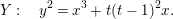
Proposition 6.1. Let
 $X$
be the K3 surface over
$X$
be the K3 surface over
 $\mathbb{C}$
defined by the Weierstrass equation
$\mathbb{C}$
defined by the Weierstrass equation
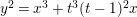
 $$\begin{eqnarray}X:\quad y^{2}=x^{3}+t^{3}(t-1)^{2}x.\end{eqnarray}$$
Then, its Néron–Severi group is generated by fiber components, the zero section and the 2-torsion section
 $Q=(0,0)$
. It is of rank 20 and determinant
$Q=(0,0)$
. It is of rank 20 and determinant
 $-4$
.
$-4$
.
Proof. By the theory of Mordell–Weil lattices,
 $NS(X)$
is spanned by fiber components and sections. The elliptic fibration has
$NS(X)$
is spanned by fiber components and sections. The elliptic fibration has
 $j$
-invariant equal to 1728 and discriminant
$j$
-invariant equal to 1728 and discriminant
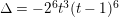
 $\unicode[STIX]{x1D6E5}=-2^{6}t^{9}(t-1)^{6}$
. Using the classification of singular fibers by Kodaira and Tate, we get that the fibration has two fibers of type
$\unicode[STIX]{x1D6E5}=-2^{6}t^{9}(t-1)^{6}$
. Using the classification of singular fibers by Kodaira and Tate, we get that the fibration has two fibers of type
 $\mathit{III}^{\ast }$
over
$\mathit{III}^{\ast }$
over
 $t=0,\infty$
and one fiber of type
$t=0,\infty$
and one fiber of type
 $I_{0}^{\ast }$
over
$I_{0}^{\ast }$
over
 $t=1$
. Hence, the trivial lattice
$t=1$
. Hence, the trivial lattice
 $L$
is of the form
$L$
is of the form
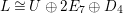 $L\cong U\oplus 2E_{7}\oplus D_{4}$
. Since it is of the maximum possible rank 20, the fibration admits no section of infinite order. The determinant
$L\cong U\oplus 2E_{7}\oplus D_{4}$
. Since it is of the maximum possible rank 20, the fibration admits no section of infinite order. The determinant
 $-16$
of the trivial lattice implies that only 2- or 4-torsion may appear. Obviously,
$-16$
of the trivial lattice implies that only 2- or 4-torsion may appear. Obviously,
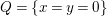 $Q=\{x=y=0\}$
is the only 2-torsion section, and 4-torsion may not occur due to the singular fibers. Alternatively, the reader may note that additional torsion turns
$Q=\{x=y=0\}$
is the only 2-torsion section, and 4-torsion may not occur due to the singular fibers. Alternatively, the reader may note that additional torsion turns
 $NS(X)$
into a unimodular lattice of signature
$NS(X)$
into a unimodular lattice of signature
 $(1,19)$
. Such a lattice does not exist.◻
$(1,19)$
. Such a lattice does not exist.◻
Note that the
 $j$
-invariant
$j$
-invariant
 $j=1728$
is constant. Hence, all smooth fibers are isomorphic – such a fibration is called isotrivial.
$j=1728$
is constant. Hence, all smooth fibers are isomorphic – such a fibration is called isotrivial.
Proposition 6.2. For
 $p\equiv 3~\text{mod}\,4$
, the surface
$p\equiv 3~\text{mod}\,4$
, the surface
 $X(p):=X\otimes \overline{\mathbb{F}}_{p}$
is the supersingular K3 surface of Artin invariant one.
$X(p):=X\otimes \overline{\mathbb{F}}_{p}$
is the supersingular K3 surface of Artin invariant one.
Proof. The singular K3 surface
 $X$
has good reduction at
$X$
has good reduction at
 $p\neq 2$
and
$p\neq 2$
and
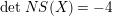 $\det NS(X)=-4$
. A prime
$\det NS(X)=-4$
. A prime
 $p$
is inert in
$p$
is inert in
 $\mathbb{Q}(\sqrt{-1})$
if and only if
$\mathbb{Q}(\sqrt{-1})$
if and only if
 $p\equiv 3~\text{mod}\,4$
. Thus, by Proposition 2.1, for all
$p\equiv 3~\text{mod}\,4$
. Thus, by Proposition 2.1, for all
 $p\equiv 3~\text{mod}\,4$
, the K3 surface
$p\equiv 3~\text{mod}\,4$
, the K3 surface
 $X(p):=X\otimes \overline{\mathbb{F}}_{p}$
is supersingular; that is,
$X(p):=X\otimes \overline{\mathbb{F}}_{p}$
is supersingular; that is,
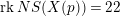 $\text{rk}\,NS(X(p))=22$
. It is known that
$\text{rk}\,NS(X(p))=22$
. It is known that
 $NS(X(p))$
is a
$NS(X(p))$
is a
 $p$
-elementary lattice of determinant
$p$
-elementary lattice of determinant
 $-p^{2\unicode[STIX]{x1D70E}}$
, where
$-p^{2\unicode[STIX]{x1D70E}}$
, where
 $\unicode[STIX]{x1D70E}\in \{1,\ldots ,10\}$
is called the Artin invariant of
$\unicode[STIX]{x1D70E}\in \{1,\ldots ,10\}$
is called the Artin invariant of
 $X(p)$
. Following an argument by Shimada [Reference Shimada14], we show that
$X(p)$
. Following an argument by Shimada [Reference Shimada14], we show that
 $\unicode[STIX]{x1D70E}=1$
. Via specialization, we get an embedding
$\unicode[STIX]{x1D70E}=1$
. Via specialization, we get an embedding
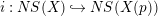 $i:NS(X){\hookrightarrow}NS(X(p))$
. Therefore,
$i:NS(X){\hookrightarrow}NS(X(p))$
. Therefore,
 $NS(X)\oplus i(NS(X))^{\bot }{\hookrightarrow}NS(X(p))$
. Since
$NS(X)\oplus i(NS(X))^{\bot }{\hookrightarrow}NS(X(p))$
. Since
 $p\neq 2$
, the
$p\neq 2$
, the
 $p$
-part of
$p$
-part of
 $A_{NS(X)\oplus i(NS(X))^{\bot }}=A_{NS(X)}\oplus A_{i(NS(X))^{\bot }}$
equals that of
$A_{NS(X)\oplus i(NS(X))^{\bot }}=A_{NS(X)}\oplus A_{i(NS(X))^{\bot }}$
equals that of
 $A_{i(NS(X))^{\bot }}$
. Hence, it is of length at most two. However, the
$A_{i(NS(X))^{\bot }}$
. Hence, it is of length at most two. However, the
 $p$
-part of
$p$
-part of
 $A_{NS(X(p))}$
is a subquotient of this. We conclude that its
$A_{NS(X(p))}$
is a subquotient of this. We conclude that its
 $p$
-part has length at most two. On the other hand,
$p$
-part has length at most two. On the other hand,
 $\unicode[STIX]{x1D70E}\in \{1,\ldots ,10\}$
, which implies that
$\unicode[STIX]{x1D70E}\in \{1,\ldots ,10\}$
, which implies that
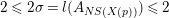 $2\leqslant 2\unicode[STIX]{x1D70E}=l(A_{NS(X(p))})\leqslant 2$
.◻
$2\leqslant 2\unicode[STIX]{x1D70E}=l(A_{NS(X(p))})\leqslant 2$
.◻
Our next task is to work out generators of
 $NS(X(p))$
for
$NS(X(p))$
for
 $p\equiv 3~\text{mod}\,4$
. By Theorem 5.1, it is generated by sections and fiber components. Reducing
$p\equiv 3~\text{mod}\,4$
. By Theorem 5.1, it is generated by sections and fiber components. Reducing
 $j$
and
$j$
and
 $\unicode[STIX]{x1D6E5}~\text{mod}\,p$
, we see that the fiber types are preserved mod
$\unicode[STIX]{x1D6E5}~\text{mod}\,p$
, we see that the fiber types are preserved mod
 $p$
(even in case
$p$
(even in case
 $p=3$
; cf. [Reference Silverman16, p. 365]). Hence, sections of infinite order must appear. Generally, it is hard to compute sections of an elliptic fibration. For this special fibration, there is a trick involving a purely inseparable base change of degree
$p=3$
; cf. [Reference Silverman16, p. 365]). Hence, sections of infinite order must appear. Generally, it is hard to compute sections of an elliptic fibration. For this special fibration, there is a trick involving a purely inseparable base change of degree
 $p$
turning
$p$
turning
 $X(p)$
into a Zariski surface.
$X(p)$
into a Zariski surface.
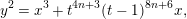
Proposition 6.3. Let
 $p=4n+3$
be a prime number. Then, the Néron–Severi group of
$p=4n+3$
be a prime number. Then, the Néron–Severi group of
 $X(p)$
defined by
$X(p)$
defined by
 $y^{2}=x^{3}+t^{3}(t-1)^{2}x$
over
$y^{2}=x^{3}+t^{3}(t-1)^{2}x$
over
 $\overline{\mathbb{F}}_{p}$
is generated by the sections
$\overline{\mathbb{F}}_{p}$
is generated by the sections
 $O,Q,P,R$
and fiber components, where
$O,Q,P,R$
and fiber components, where
 $O$
denotes the section at infinity,
$O$
denotes the section at infinity,
 $Q=(0,0)$
is the 2-torsion section,
$Q=(0,0)$
is the 2-torsion section,
 $\unicode[STIX]{x1D701}^{4}=-1$
and
$\unicode[STIX]{x1D701}^{4}=-1$
and
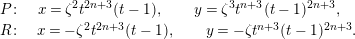 $$\begin{eqnarray}\begin{array}{@{}l@{}}P:\quad x=\unicode[STIX]{x1D701}^{2}t^{2n+3}(t-1),\qquad y=\unicode[STIX]{x1D701}^{3}t^{n+3}(t-1)^{2n+3},\\ R:\quad x=-\unicode[STIX]{x1D701}^{2}t^{2n+3}(t-1),\qquad y=-\unicode[STIX]{x1D701}t^{n+3}(t-1)^{2n+3}.\end{array}\end{eqnarray}$$
We have the following intersection numbers, symmetric in
 $P$
and
$P$
and
 $R$
:
$R$
:
 $$\begin{eqnarray}O.P=Q.P=O.R=Q.R=n,\quad P.R=2n.\end{eqnarray}$$
Proof. One can check directly that
 $P$
and
$P$
and
 $R$
are sections of the elliptic fibration, and the patient reader may calculate their intersection numbers by hand. Since
$R$
are sections of the elliptic fibration, and the patient reader may calculate their intersection numbers by hand. Since
 $X(p)$
has Artin invariant
$X(p)$
has Artin invariant
 $\unicode[STIX]{x1D70E}=1$
,
$\unicode[STIX]{x1D70E}=1$
,
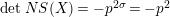 $\det NS(X)=-p^{2\unicode[STIX]{x1D70E}}=-p^{2}$
. All that remains is to compute the intersection matrix of these four sections and the fiber components. One can check that it has a
$\det NS(X)=-p^{2\unicode[STIX]{x1D70E}}=-p^{2}$
. All that remains is to compute the intersection matrix of these four sections and the fiber components. One can check that it has a
 $22\times 22$
minor of determinant
$22\times 22$
minor of determinant
 $-p^{2}$
. This minor corresponds to a basis of
$-p^{2}$
. This minor corresponds to a basis of
 $NS(X(p))$
.◻
$NS(X(p))$
.◻
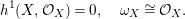
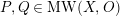
For later reference, we fix the following
 $\mathbb{Z}$
-basis of the Néron–Severi group, where the fiber components are sorted as indicated in Figure 1, and
$\mathbb{Z}$
-basis of the Néron–Severi group, where the fiber components are sorted as indicated in Figure 1, and
 $e_{20}$
is distinguished by
$e_{20}$
is distinguished by
 $e_{20}.P=1$
:
$e_{20}.P=1$
:
 $$\begin{eqnarray}(O,F,Q,E_{7}(t=\infty ),E_{7}(t=0),A_{3}(\subseteq D_{4},t=1),e_{21}=P,e_{22}=R).\end{eqnarray}$$
Blue vertexes and edges belong to fibers. Replacing
 $Q$
by one of the missing components of the
$Q$
by one of the missing components of the
 $I_{0}^{\ast }$
fiber results in a
$I_{0}^{\ast }$
fiber results in a
 $\mathbb{Q}$
- instead of a
$\mathbb{Q}$
- instead of a
 $\mathbb{Z}$
-basis. This is predicted by Theorem 5.1.
$\mathbb{Z}$
-basis. This is predicted by Theorem 5.1.

Figure 1. Twenty-four
 $(-2)$
-curves of
$(-2)$
-curves of
 $X$
supporting singular fibers of type
$X$
supporting singular fibers of type
 $I_{0}^{\ast },2\times \mathit{III}^{\ast }$
(blue) and torsion sections of
$I_{0}^{\ast },2\times \mathit{III}^{\ast }$
(blue) and torsion sections of
 $\unicode[STIX]{x1D70B}$
.
$\unicode[STIX]{x1D70B}$
.
For the intersection matrix in this basis, one obtains
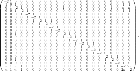 $$\begin{eqnarray}\left(\begin{smallmatrix}-2 & 1 & 0 & 0 & 0 & 0 & 0 & 0 & 0 & 0 & 0 & 0 & 0 & 0 & 0 & 0 & 0 & 0 & 0 & 0 & n & n\\ 1 & 0 & 1 & 0 & 0 & 0 & 0 & 0 & 0 & 0 & 0 & 0 & 0 & 0 & 0 & 0 & 0 & 0 & 0 & 0 & 1 & 1\\ 0 & 1 & -2 & 1 & 0 & 0 & 0 & 0 & 0 & 0 & 1 & 0 & 0 & 0 & 0 & 0 & 0 & 0 & 1 & 0 & n & n\\ 0 & 0 & 1 & -2 & 1 & 0 & 0 & 0 & 0 & 0 & 0 & 0 & 0 & 0 & 0 & 0 & 0 & 0 & 0 & 0 & 1 & 1\\ 0 & 0 & 0 & 1 & -2 & 1 & 0 & 0 & 0 & 0 & 0 & 0 & 0 & 0 & 0 & 0 & 0 & 0 & 0 & 0 & 0 & 0\\ 0 & 0 & 0 & 0 & 1 & -2 & 1 & 0 & 0 & 0 & 0 & 0 & 0 & 0 & 0 & 0 & 0 & 0 & 0 & 0 & 0 & 0\\ 0 & 0 & 0 & 0 & 0 & 1 & -2 & 1 & 1 & 0 & 0 & 0 & 0 & 0 & 0 & 0 & 0 & 0 & 0 & 0 & 0 & 0\\ 0 & 0 & 0 & 0 & 0 & 0 & 1 & -2 & 0 & 0 & 0 & 0 & 0 & 0 & 0 & 0 & 0 & 0 & 0 & 0 & 0 & 0\\ 0 & 0 & 0 & 0 & 0 & 0 & 1 & 0 & -2 & 1 & 0 & 0 & 0 & 0 & 0 & 0 & 0 & 0 & 0 & 0 & 0 & 0\\ 0 & 0 & 0 & 0 & 0 & 0 & 0 & 0 & 1 & -2 & 0 & 0 & 0 & 0 & 0 & 0 & 0 & 0 & 0 & 0 & 0 & 0\\ 0 & 0 & 1 & 0 & 0 & 0 & 0 & 0 & 0 & 0 & -2 & 1 & 0 & 0 & 0 & 0 & 0 & 0 & 0 & 0 & 0 & 0\\ 0 & 0 & 0 & 0 & 0 & 0 & 0 & 0 & 0 & 0 & 1 & -2 & 1 & 0 & 0 & 0 & 0 & 0 & 0 & 0 & 0 & 0\\ 0 & 0 & 0 & 0 & 0 & 0 & 0 & 0 & 0 & 0 & 0 & 1 & -2 & 1 & 0 & 0 & 0 & 0 & 0 & 0 & 0 & 0\\ 0 & 0 & 0 & 0 & 0 & 0 & 0 & 0 & 0 & 0 & 0 & 0 & 1 & -2 & 1 & 1 & 0 & 0 & 0 & 0 & 0 & 0\\ 0 & 0 & 0 & 0 & 0 & 0 & 0 & 0 & 0 & 0 & 0 & 0 & 0 & 1 & -2 & 0 & 0 & 0 & 0 & 0 & 0 & 0\\ 0 & 0 & 0 & 0 & 0 & 0 & 0 & 0 & 0 & 0 & 0 & 0 & 0 & 1 & 0 & -2 & 1 & 0 & 0 & 0 & 0 & 0\\ 0 & 0 & 0 & 0 & 0 & 0 & 0 & 0 & 0 & 0 & 0 & 0 & 0 & 0 & 0 & 1 & -2 & 0 & 0 & 0 & 0 & 0\\ 0 & 0 & 0 & 0 & 0 & 0 & 0 & 0 & 0 & 0 & 0 & 0 & 0 & 0 & 0 & 0 & 0 & -2 & 1 & 1 & 0 & 0\\ 0 & 0 & 1 & 0 & 0 & 0 & 0 & 0 & 0 & 0 & 0 & 0 & 0 & 0 & 0 & 0 & 0 & 1 & -2 & 0 & 0 & 0\\ 0 & 0 & 0 & 0 & 0 & 0 & 0 & 0 & 0 & 0 & 0 & 0 & 0 & 0 & 0 & 0 & 0 & 1 & 0 & -2 & 1 & 0\\ n & 1 & n & 1 & 0 & 0 & 0 & 0 & 0 & 0 & 0 & 0 & 0 & 0 & 0 & 0 & 0 & 0 & 0 & 1 & -2 & 2n\\ n & 1 & n & 1 & 0 & 0 & 0 & 0 & 0 & 0 & 0 & 0 & 0 & 0 & 0 & 0 & 0 & 0 & 0 & 0 & 2n & -2\end{smallmatrix}\right).\end{eqnarray}$$
In the remaining part of this section, we explain how the sections
 $P,R$
are found and give an alternative way of computing their intersection numbers.
$P,R$
are found and give an alternative way of computing their intersection numbers.
Recall that we assume that
 $p\equiv 3~\text{mod}\,4$
and write
$p\equiv 3~\text{mod}\,4$
and write
 $p=4n+3$
. Consider the purely inseparable base change
$p=4n+3$
. Consider the purely inseparable base change
 $t\mapsto t^{p}$
. This changes the equation as follows:
$t\mapsto t^{p}$
. This changes the equation as follows:
 $$\begin{eqnarray}y^{2}=x^{3}+t^{12n+9}(t-1)^{8n+6}x.\end{eqnarray}$$
We minimize this equation using the birational map
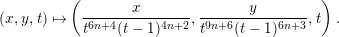 $$\begin{eqnarray}(x,y,t)\mapsto \left(\frac{x}{t^{6n+4}(t-1)^{4n+2}},\frac{y}{t^{9n+6}(t-1)^{6n+3}},t\right).\end{eqnarray}$$
This leads to the surface
 $Y$
given by
$Y$
given by
 $$\begin{eqnarray}Y:\quad y^{2}=x^{3}+t(t-1)^{2}x.\end{eqnarray}$$
After another base change
 $t\mapsto t^{p}$
, we get
$t\mapsto t^{p}$
, we get
 $$\begin{eqnarray}y^{2}=x^{3}+t^{4n+3}(t-1)^{8n+6}x,\end{eqnarray}$$
and minimizing the fibration
 $$\begin{eqnarray}\left(\frac{y}{t^{3n}(t-1)^{6n+3}}\right)^{2}=\left(\frac{x}{t^{2n}(t-1)^{4n+2}}\right)^{3}+t^{3}(t-1)^{2}\frac{x}{t^{2n}(t-1)^{4n+2}},\end{eqnarray}$$
we recover
 $X$
.
$X$
.
Instead of directly searching for sections on
 $X$
, we exhibit two sections on
$X$
, we exhibit two sections on
 $Y$
and pull them back to
$Y$
and pull them back to
 $X$
. The
$X$
. The
 $j$
-invariant of
$j$
-invariant of
 $Y$
is still equal to 1728, but
$Y$
is still equal to 1728, but
 $\unicode[STIX]{x1D6E5}=-2^{6}t^{3}(t-1)^{6}$
. For
$\unicode[STIX]{x1D6E5}=-2^{6}t^{3}(t-1)^{6}$
. For
 $p\neq 3$
, this leads to two singular fibers of type
$p\neq 3$
, this leads to two singular fibers of type
 $\mathit{III}$
over
$\mathit{III}$
over
 $t=0,\infty$
and a singular fiber of type
$t=0,\infty$
and a singular fiber of type
 $I_{0}^{\ast }$
over
$I_{0}^{\ast }$
over
 $t=1$
. The Euler number of this surface is
$t=1$
. The Euler number of this surface is
 $2e(\mathit{III})+e(I_{0}^{\ast })=2\cdot 3+6=12$
. By general theory, it is rational. The trivial lattice is isomorphic to
$2e(\mathit{III})+e(I_{0}^{\ast })=2\cdot 3+6=12$
. By general theory, it is rational. The trivial lattice is isomorphic to
 $$\begin{eqnarray}\text{Triv}(Y)\cong U\oplus 2A_{1}\oplus D_{4}.\end{eqnarray}$$
This lattice is of determinant
 $-16$
and rank 8. From the theory of elliptically fibered rational surfaces, we know that
$-16$
and rank 8. From the theory of elliptically fibered rational surfaces, we know that
 $\text{rk}\,NS(Y)=10$
,
$\text{rk}\,NS(Y)=10$
,
 $\det NS(Y)=-1$
, which implies that
$\det NS(Y)=-1$
, which implies that
 $Y$
has Mordell–Weil rank 2. Define
$Y$
has Mordell–Weil rank 2. Define
 $$\begin{eqnarray}\text{Triv}^{\prime }(Y):=\text{Triv}(Y)\otimes _{\mathbb{ Z}}\mathbb{Q}\cap NS(Y).\end{eqnarray}$$
Then, by Theorem 5.1,
 $\text{Triv}^{\prime }(Y)/\text{Triv}(Y)\cong \text{MW}_{tors}$
. Since
$\text{Triv}^{\prime }(Y)/\text{Triv}(Y)\cong \text{MW}_{tors}$
. Since
 $\{x=y=0\}$
is a 2-torsion section, we know that
$\{x=y=0\}$
is a 2-torsion section, we know that
 $$\begin{eqnarray}\det \text{Triv}^{\prime }(Y)=\det \text{Triv}(Y)/[\text{Triv}^{\prime }(Y):\text{Triv}(Y)]^{2}\in \{-1,-4\}.\end{eqnarray}$$
As even unimodular lattices of signature
 $(1,7)$
do not exist,
$(1,7)$
do not exist,
 $-1$
is impossible. We conclude that
$-1$
is impossible. We conclude that
 $x=y=0$
is the only torsion section.
$x=y=0$
is the only torsion section.
To find a section of infinite order, we first determine the Mordell–Weil lattice and then translate this information to equations of the section. Since
 $j=1728$
, the elliptic curve admits complex multiplication given by
$j=1728$
, the elliptic curve admits complex multiplication given by
 $(x,y)\mapsto (-x,iy)$
. Obviously,
$(x,y)\mapsto (-x,iy)$
. Obviously,
 $Q$
and
$Q$
and
 $O$
are the unique sections fixed by this action. Hence, the Mordell–Weil lattice admits an isometry of order four, which, viewed as an element of
$O$
are the unique sections fixed by this action. Hence, the Mordell–Weil lattice admits an isometry of order four, which, viewed as an element of
 $O(2)$
, may only be a rotation by
$O(2)$
, may only be a rotation by
 $\pm {\textstyle \frac{\unicode[STIX]{x1D70B}}{2}}$
. Up to isometry, all positive definite lattices of rank 2 admitting an isometry of order four have a Gram matrix of the form
$\pm {\textstyle \frac{\unicode[STIX]{x1D70B}}{2}}$
. Up to isometry, all positive definite lattices of rank 2 admitting an isometry of order four have a Gram matrix of the form
 $$\begin{eqnarray}\left(\begin{array}{@{}cc@{}}a & 0\\ 0 & a\end{array}\right)\end{eqnarray}$$
for some
 $a>0$
. The formula
$a>0$
. The formula
 $$\begin{eqnarray}\det NS(Y)=(-1)^{r}\det \text{MWL}(Y)\det \text{Triv}^{\prime }(Y),\end{eqnarray}$$
where
 $r=rk\,\text{MWL}(Y)=2$
,
$r=rk\,\text{MWL}(Y)=2$
,
 $\det NS(Y)=-1$
,
$\det NS(Y)=-1$
,
 $\det \text{Triv}^{\prime }(Y)=4$
, resulting from the definition of
$\det \text{Triv}^{\prime }(Y)=4$
, resulting from the definition of
 $\text{MWL}(Y)$
via the orthogonal projection with respect to
$\text{MWL}(Y)$
via the orthogonal projection with respect to
 $\text{Triv}^{\prime }(Y)$
, yields
$\text{Triv}^{\prime }(Y)$
, yields
 $a=1/2$
.
$a=1/2$
.
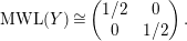 $$\begin{eqnarray}\text{MWL}(Y)\cong \left(\begin{array}{@{}cc@{}}1/2 & 0\\ 0 & 1/2\end{array}\right).\end{eqnarray}$$
We search for a section
 $P$
with
$P$
with
 $$\begin{eqnarray}1/2=\langle P,P\rangle :=2\unicode[STIX]{x1D712}+2P.O-c_{0}(P,P)-c_{\infty }(P,P)-c_{1}(P,P),\end{eqnarray}$$
where
 $\unicode[STIX]{x1D712}=\unicode[STIX]{x1D712}({\mathcal{O}}_{Y})=1$
is the Euler characteristic of
$\unicode[STIX]{x1D712}=\unicode[STIX]{x1D712}({\mathcal{O}}_{Y})=1$
is the Euler characteristic of
 $Y$
and
$Y$
and
 $c_{0},c_{\infty }\in \{0,1/2\},c_{1}\in \{0,1\}$
are the contributions at the singular fibers;
$c_{0},c_{\infty }\in \{0,1/2\},c_{1}\in \{0,1\}$
are the contributions at the singular fibers;
 $P.O\in \mathbb{N}$
is the intersection number. This immediately implies
$P.O\in \mathbb{N}$
is the intersection number. This immediately implies
 $P.O=0$
and
$P.O=0$
and
 $c_{1}=1$
. Let us assume
$c_{1}=1$
. Let us assume
 $c_{0}=1/2,c_{\infty }=0$
. The section
$c_{0}=1/2,c_{\infty }=0$
. The section
 $P$
can be given by
$P$
can be given by
 $(x(t),y(t))$
, where
$(x(t),y(t))$
, where
 $x,y$
are rational functions. Over the chart containing
$x,y$
are rational functions. Over the chart containing
 $\infty$
, it is given by
$\infty$
, it is given by
 $(\hat{x}(s),{\hat{y}}(s))=(s^{2}x(1/s),s^{3}y(1/s))$
, where
$(\hat{x}(s),{\hat{y}}(s))=(s^{2}x(1/s),s^{3}y(1/s))$
, where
 $s=1/t$
. As poles of these functions correspond to intersections with the zero section, we know that
$s=1/t$
. As poles of these functions correspond to intersections with the zero section, we know that
 $x,y,\hat{x},{\hat{y}}$
are actually polynomials. Therefore,
$x,y,\hat{x},{\hat{y}}$
are actually polynomials. Therefore,
 $\deg x\leqslant 2$
and
$\deg x\leqslant 2$
and
 $\deg y\leqslant 3$
. Furthermore, if
$\deg y\leqslant 3$
. Furthermore, if
 $P$
intersects the same fiber component as the zero section, then the contribution
$P$
intersects the same fiber component as the zero section, then the contribution
 $c_{\unicode[STIX]{x1D708}}$
of that fiber is zero. The other components arise by blowing up the singularities of the Weierstraß model in
$c_{\unicode[STIX]{x1D708}}$
of that fiber is zero. The other components arise by blowing up the singularities of the Weierstraß model in
 $\{x=y=t(t-1)=0\}$
. Hence,
$\{x=y=t(t-1)=0\}$
. Hence,
 $x(0)=y(0)=x(1)=y(1)=0$
. Putting this information together, we obtain
$x(0)=y(0)=x(1)=y(1)=0$
. Putting this information together, we obtain
 $x=at(t-1)$
and
$x=at(t-1)$
and
 $y=t(t-1)b$
for some constant
$y=t(t-1)b$
for some constant
 $a$
and a polynomial
$a$
and a polynomial
 $b(x)$
of degree one. A quick calculation yields the sections
$b(x)$
of degree one. A quick calculation yields the sections
 $$\begin{eqnarray}\displaystyle & \displaystyle P^{\prime }:\quad x(t)=\unicode[STIX]{x1D701}^{2}t(t-1),\qquad y(t)=\unicode[STIX]{x1D701}^{3}t(t-1)^{2}, & \displaystyle\end{eqnarray}$$
 $$\begin{eqnarray}\displaystyle & \displaystyle R^{\prime }:\quad x(t)=-\unicode[STIX]{x1D701}^{2}t(t-1),\qquad y(t)=-\unicode[STIX]{x1D701}t(t-1)^{2}, & \displaystyle\end{eqnarray}$$
for
 $\unicode[STIX]{x1D701}^{4}+1=0$
. Note that
$\unicode[STIX]{x1D701}^{4}+1=0$
. Note that
 $\text{MWL}(Y)$
contains exactly four sections of height
$\text{MWL}(Y)$
contains exactly four sections of height
 $1/2$
. Furthermore,
$1/2$
. Furthermore,
 $\langle P^{\prime },R^{\prime }\rangle =0$
. (Otherwise,
$\langle P^{\prime },R^{\prime }\rangle =0$
. (Otherwise,
 $P=\ominus R$
, which is clearly false.) The two further Galois conjugates of
$P=\ominus R$
, which is clearly false.) The two further Galois conjugates of
 $\unicode[STIX]{x1D701}$
correspond to the missing two sections
$\unicode[STIX]{x1D701}$
correspond to the missing two sections
 $\ominus P$
and
$\ominus P$
and
 $\ominus R$
.
$\ominus R$
.
Now we pull back
 $P^{\prime }$
and
$P^{\prime }$
and
 $R^{\prime }$
to
$R^{\prime }$
to
 $X$
via the map
$X$
via the map
 $$\begin{eqnarray}\unicode[STIX]{x1D719}:\quad X\rightarrow Y,\quad (x,y,t)\mapsto (xt^{2n}(t-1)^{4n+2},yt^{3n}(t-1)^{6n+3},t^{p}),\end{eqnarray}$$
and get the sections
 $$\begin{eqnarray}\displaystyle & \displaystyle P:\quad x=\unicode[STIX]{x1D701}^{2}t^{2n+3}(t-1),\qquad y=\unicode[STIX]{x1D701}^{3}t^{n+3}(t-1)^{2n+3}, & \displaystyle\end{eqnarray}$$
 $$\begin{eqnarray}\displaystyle & \displaystyle R:\quad x=-\unicode[STIX]{x1D701}^{2}t^{2n+3}(t-1),\qquad y=-\unicode[STIX]{x1D701}t^{n+3}(t-1)^{2n+3}. & \displaystyle\end{eqnarray}$$
It remains to compute the intersection numbers involving
 $P$
and
$P$
and
 $R$
. This can be done by blowing up the singularities and then computing the intersections. However, by applying some more of Shioda’s theory, we can avoid the blowing up. From the behavior of the height pairing under base extension (cf. [Reference Shioda13, Proposition 8.12]), we know that
$R$
. This can be done by blowing up the singularities and then computing the intersections. However, by applying some more of Shioda’s theory, we can avoid the blowing up. From the behavior of the height pairing under base extension (cf. [Reference Shioda13, Proposition 8.12]), we know that
 $$\begin{eqnarray}\langle P,P\rangle =\deg \unicode[STIX]{x1D719}\langle P^{\prime },P^{\prime }\rangle =p\langle P^{\prime },P^{\prime }\rangle =2n+3/2,\end{eqnarray}$$
and get the equation
 $$\begin{eqnarray}2n+3/2=4+2P.O-c_{0}(P,P)-c_{\infty }(P,P)-c_{1}(P,P).\end{eqnarray}$$
Note that a fiber of type
 $\mathit{III}^{\ast }$
has only two simple components. Since
$\mathit{III}^{\ast }$
has only two simple components. Since
 $P$
meets the same component over infinity as the zero section and passes through the singularities at
$P$
meets the same component over infinity as the zero section and passes through the singularities at
 $t=0,1$
, we know that
$t=0,1$
, we know that
 $c_{\infty }=0$
,
$c_{\infty }=0$
,
 $c_{0}=3/2$
and
$c_{0}=3/2$
and
 $c_{1}=1$
. We conclude that
$c_{1}=1$
. We conclude that
 $P.O=n$
. The other intersection numbers can be calculated accordingly. In this way, we could calculate the intersection matrix of
$P.O=n$
. The other intersection numbers can be calculated accordingly. In this way, we could calculate the intersection matrix of
 $NS(X(p))$
without knowing equations for the extra sections.
$NS(X(p))$
without knowing equations for the extra sections.
The section
 $P$
induces an automorphism of the surface by fiberwise addition. We denote it by
$P$
induces an automorphism of the surface by fiberwise addition. We denote it by
 $(\oplus P)$
. The matrix of its representation on
$(\oplus P)$
. The matrix of its representation on
 $NS$
is obtained as follows.
$NS$
is obtained as follows.
-
∙ Compute the basis representation of the sections
$Q\oplus P,2P$
and
$R\oplus P$
. -
∙ Any section
$S$
is mapped to
$P\oplus S$
under
$(\oplus P)_{\ast }$
, and the fiber is fixed. -
∙ The action of
$(\oplus P)$
on the Néron–Severi group preserves each singular fiber. Since it is an isometry, it can be determined by its action on sections. -
∙ Invert the resulting matrix to get
$(\oplus P)^{\ast }=(\oplus P)_{\ast }^{-1}$
.


A basis representation of
 $P\oplus Q$
is obtained as follows. Start with
$P\oplus Q$
is obtained as follows. Start with
 $P+Q\in NS$
and subtract
$P+Q\in NS$
and subtract
 $nO$
, such that the resulting divisor
$nO$
, such that the resulting divisor
 $D$
has
$D$
has
 $D.F=1$
. Add or subtract fiber components until
$D.F=1$
. Add or subtract fiber components until
 $D$
meets each singular fiber in exactly one simple component. Finally, add multiples of
$D$
meets each singular fiber in exactly one simple component. Finally, add multiples of
 $F$
such that
$F$
such that
 $D^{2}=-2$
. For example, the basis representation of the section
$D^{2}=-2$
. For example, the basis representation of the section
 $P\oplus R$
is given by
$P\oplus R$
is given by
 $$\begin{eqnarray}(1,2,-2,0,0,0,0,0,0,0,-3,-4,-5,-6,-3,-4,-2,-1,-2,0,1,1).\end{eqnarray}$$
7 Alternative elliptic fibrations
The automorphism constructed in the last section has zero entropy. The reason for this is that it fixes the fibers. We overcome this obstruction by combining different fibrations and their sections.
Reducible singular fibers of elliptic fibrations are extended
 $ADE$
-configurations of
$ADE$
-configurations of
 $(-2)$
-curves. Conversely, let
$(-2)$
-curves. Conversely, let
 $X$
be a K3 surface, and let
$X$
be a K3 surface, and let
 $F$
be an extended
$F$
be an extended
 $ADE$
-configuration of
$ADE$
-configuration of
 $(-2)$
-curves. Then, the linear system
$(-2)$
-curves. Then, the linear system
 $|F|$
is an elliptic pencil with the extended
$|F|$
is an elliptic pencil with the extended
 $ADE$
-configuration as singular fiber. See [Reference Kondō8] and [Reference Pjateckiĭ-Šapiro and Šafarevič11] for details. We use this fact to detect additional elliptic fibrations in the graph of
$ADE$
-configuration as singular fiber. See [Reference Kondō8] and [Reference Pjateckiĭ-Šapiro and Šafarevič11] for details. We use this fact to detect additional elliptic fibrations in the graph of
 $(-2)$
-curves. Irreducible curves
$(-2)$
-curves. Irreducible curves
 $C$
are either fiber components, sections or multisections, depending on whether
$C$
are either fiber components, sections or multisections, depending on whether
 $C.F=0,1$
or
$C.F=0,1$
or
 ${>}1$
. Be aware that the
${>}1$
. Be aware that the
 $(-2)$
-curves occur with multiplicities in
$(-2)$
-curves occur with multiplicities in
 $F$
. Hence, it is possible that
$F$
. Hence, it is possible that
 $C.F>1$
even if
$C.F>1$
even if
 $C$
meets only a single
$C$
meets only a single
 $(-2)$
-curve of the configuration. In general, an elliptic pencil does not necessarily admit a section. However, once its existence is guaranteed, we may choose it as zero section. Then, by Theorem 5.1, multisections still induce sections once modified by fiber components and the zero section, as sketched above.
$(-2)$
-curve of the configuration. In general, an elliptic pencil does not necessarily admit a section. However, once its existence is guaranteed, we may choose it as zero section. Then, by Theorem 5.1, multisections still induce sections once modified by fiber components and the zero section, as sketched above.

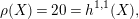
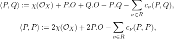
Figure 2.
 $\unicode[STIX]{x1D70B}^{\prime }$
with
$\unicode[STIX]{x1D70B}^{\prime }$
with
 $I_{16}$
and
$I_{16}$
and
 $I_{4}$
fibers and
$I_{4}$
fibers and
 $\unicode[STIX]{x1D70B}^{\prime \prime }$
with
$\unicode[STIX]{x1D70B}^{\prime \prime }$
with
 $I_{12}$
and
$I_{12}$
and
 $IV^{\ast }$
fibers.
$IV^{\ast }$
fibers.
The first fibration
 $\unicode[STIX]{x1D70B}^{\prime }$
is induced by the outer circle of
$\unicode[STIX]{x1D70B}^{\prime }$
is induced by the outer circle of
 $(-2)$
-curves, which is a singular fiber of type
$(-2)$
-curves, which is a singular fiber of type
 $I_{16}$
. There is a second singular fiber of type
$I_{16}$
. There is a second singular fiber of type
 $I_{4}$
. Three of its components are visible in Figure 2. The curve
$I_{4}$
. Three of its components are visible in Figure 2. The curve
 $e_{8}$
(
$e_{8}$
(
 $=$
vertex labeled by “8”) is a section since it meets
$=$
vertex labeled by “8”) is a section since it meets
 $I_{16}$
exactly in a simple component. We take it as zero section. Then, the torsion sections are
$I_{16}$
exactly in a simple component. We take it as zero section. Then, the torsion sections are
 $e_{15},e_{18}$
and
$e_{15},e_{18}$
and
 $e_{19}$
. The second fibration
$e_{19}$
. The second fibration
 $\unicode[STIX]{x1D70B}^{\prime \prime }$
is induced by the right inner circle of
$\unicode[STIX]{x1D70B}^{\prime \prime }$
is induced by the right inner circle of
 $(-2)$
-curves. It has singular fibers of type
$(-2)$
-curves. It has singular fibers of type
 $I_{12}$
and
$I_{12}$
and
 $IV^{\ast }$
, and again we take
$IV^{\ast }$
, and again we take
 $e_{8}$
as zero section. A simple component of the
$e_{8}$
as zero section. A simple component of the
 $IV^{\ast }$
fiber is not visible in Figure 2. In both cases,
$IV^{\ast }$
fiber is not visible in Figure 2. In both cases,
 $P$
is a multisection and induces a section of each fibration denoted by
$P$
is a multisection and induces a section of each fibration denoted by
 $P^{\prime }$
and
$P^{\prime }$
and
 $P^{\prime \prime }$
. For example, the class of
$P^{\prime \prime }$
. For example, the class of
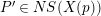 $P^{\prime }\in NS(X(p))$
is given by
$P^{\prime }\in NS(X(p))$
is given by
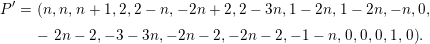 $$\begin{eqnarray}\displaystyle P^{\prime } & = & \displaystyle \left(n,n,n+1,2,2-n,-2n+2,2-3n,1-2n,1-2n,-n,0,\right.\nonumber\\ \displaystyle & & \displaystyle -\left.2n-2,-3-3n,-2n-2,-2n-2,-1-n,0,0,0,1,0\right)\!.\nonumber\end{eqnarray}$$
8 Salem degree-22 automorphism
We consider the automorphism
 $$\begin{eqnarray}f:=(\oplus R)\circ (\oplus P)\circ (\oplus P^{\prime })\circ (\oplus P^{\prime \prime })\end{eqnarray}$$
on
 $X(p)$
for
$X(p)$
for
 $p\equiv 3~\text{mod}\,4$
. Using a computer algebra system, one computes the characteristic polynomial of
$p\equiv 3~\text{mod}\,4$
. Using a computer algebra system, one computes the characteristic polynomial of
 $f^{\ast }|NS(X(p))$
:
$f^{\ast }|NS(X(p))$
:
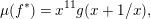 $$\begin{eqnarray}\unicode[STIX]{x1D707}(f^{\ast })=x^{11}g(x+1/x),\end{eqnarray}$$
where
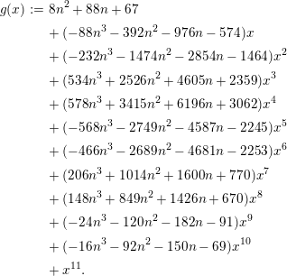 $$\begin{eqnarray}\displaystyle g(x) & := & \displaystyle 8n^{2}+88n+67\nonumber\\ \displaystyle & & \displaystyle +\,(-88n^{3}-392n^{2}-976n-574)x\nonumber\\ \displaystyle & & \displaystyle +\,(-232n^{3}-1474n^{2}-2854n-1464)x^{2}\nonumber\\ \displaystyle & & \displaystyle +\,(534n^{3}+2526n^{2}+4605n+2359)x^{3}\nonumber\\ \displaystyle & & \displaystyle +\,(578n^{3}+3415n^{2}+6196n+3062)x^{4}\nonumber\\ \displaystyle & & \displaystyle +\,(-568n^{3}-2749n^{2}-4587n-2245)x^{5}\nonumber\\ \displaystyle & & \displaystyle +\,(-466n^{3}-2689n^{2}-4681n-2253)x^{6}\nonumber\\ \displaystyle & & \displaystyle +\,(206n^{3}+1014n^{2}+1600n+770)x^{7}\nonumber\\ \displaystyle & & \displaystyle +\,(148n^{3}+849n^{2}+1426n+670)x^{8}\nonumber\\ \displaystyle & & \displaystyle +\,(-24n^{3}-120n^{2}-182n-91)x^{9}\nonumber\\ \displaystyle & & \displaystyle +\,(-16n^{3}-92n^{2}-150n-69)x^{10}\nonumber\\ \displaystyle & & \displaystyle +\,x^{11}.\nonumber\end{eqnarray}$$
By Theorem 3.1,
 $\unicode[STIX]{x1D707}(f^{\ast })$
either is a degree-22 Salem polynomial or is divisible by a cyclotomic polynomial of degree at most 22. There are only finitely many cyclotomic polynomials of a given degree. We can exclude the second case directly by computing the remainder after division for each such polynomial. This proves Theorem 1.1.
$\unicode[STIX]{x1D707}(f^{\ast })$
either is a degree-22 Salem polynomial or is divisible by a cyclotomic polynomial of degree at most 22. There are only finitely many cyclotomic polynomials of a given degree. We can exclude the second case directly by computing the remainder after division for each such polynomial. This proves Theorem 1.1.
Remark 1. Further compositions of the four automorphisms realize Salem numbers of any even degree between 2 and 22. The full matrix representations of the automorphisms
 $(\oplus R),(\oplus P),(\oplus P^{\prime }),(\oplus P^{\prime \prime })$
involved are available upon request from the author.
$(\oplus R),(\oplus P),(\oplus P^{\prime }),(\oplus P^{\prime \prime })$
involved are available upon request from the author.
Acknowledgments
I thank my advisor Matthias Schütt, who introduced me to this topic and the isotrivial fibration. Thanks to Davide Veniani and Víctor González-Alonso for discussions and helpful comments.


