


Misaligned units of analysis present challenges for users of geospatial data. Researchers studying legislative elections in the United States might observe data for variables at the electoral district level (e.g., campaign strategies) and at the county level (e.g., crime). To understand how, for example, local crime influences campaign strategies, one must integrate two datasets, using measured values at the county level to estimate levels of crime in each legislative district. Statistically, this represents a change-of-support (CoS) problem: making inferences about a variable at one geographic support (destination units) using measurements from a different support (source units). Changes of support entail information loss, potentially leading to consequential measurement error and biased estimation. Substantively, this is a general problem of mismatch between needing data at theoretically relevant levels and the reality that data may be unavailable at those levels.
How prevalent are such problems in social science? They are quite common, routinely appearing in studies of subnational (within-country) variation, where data are accessible at disparate levels of analysis, reflecting varying geographic precision, or different definitions of the same units across data sources. Units and scales (e.g., administrative areas, postal codes, and grids) do not always correspond to theoretical quantities of interest. Nor do they always relate in straightforward ways. While some units perfectly nest (e.g., U.S. counties and states), others overlap only partially (e.g., counties and legislative districts).Footnote 1
If testing the implications of theory requires data at one geographic support (e.g., electoral constituency), but theoretically relevant data exist at another support (e.g., administrative unit), researchers face consequential choices: conduct tests not commensurate with spatial levels at which theory is specified, or convert data to appropriate units. Converting data can be a messy step, which many researchers make implicitly or explicitly at some point in the data management process. We reviewed subnational empirical research in top political science journals since 2010, and found that 20% of articles, across all major subfields, change the geographic support of key variables.Footnote 2 For example, Benmelech, Berrebi and Klor (Reference Benmelech, Berrebi and Klor2015) explore relationships between house demolitions and suicide attacks in Israel by aggregating data on places of residence to the district level. Branton et al. (Reference Branton, Martinez-Ebers, Carey and Matsubayashi2015) examine impacts of protests on public opinion regarding immigration policy, combining data across multiple geographic units with county-level data on survey responses and protests. Rozenas and Zhukov (Reference Rozenas and Zhukov2019) study effects of famine on elections, protests, and violence in Ukraine, transforming several historical datasets to 1933-era Soviet districts.
It is tempting to treat changes of support as routine, similar to merging two tables by common ID. But integrating misaligned geospatial data is error-prone (Gotway and Young Reference Gotway and Young2002, Reference Gotway and Young2007; Matheron Reference Matheron and Armstrong1989), and the literature currently lacks common standards for evaluation. Much of the canonical geostatistical literature relates to geology and environmental science (e.g., Cressie Reference Cressie1996). While multiple transformation options exist (see Comber and Zeng Reference Comber and Zeng2019), there is no “silver bullet.” Despite efforts to address CoS problems in political science (Darmofal and Eddy Reference Darmofal, Eddy, Curini and Franzese2020; Donnay and Linke Reference Donnay and Linke2016; Goplerud Reference Goplerud2016; Lee and Rogers Reference Lee and Rogers2019), economics (Eckert et al. Reference Eckert, Gvirtz, Liang and Peters2020), and public health (Zhu, Waller, and Ma Reference Zhu, Waller and Ma2013), there are no prevailing best practices.
We make three contributions. First is a framework for diagnosing and addressing CoS problems involving discrete geographic areas, focusing on the relative degree of nesting (i.e., whether one set of units falls completely and neatly inside the other), and the relative scale of source and destination units (i.e., aggregation, disaggregation, and hybrid). We propose simple, nonparametric measures of nesting and scale that can help assess ex ante the complexity of transformations.
Second, we show, using examples with U.S. and Swedish electoral data, that relative nesting and scale are consequential for the performance of common spatial transformation methods, including overlays, interpolation, and kriging. Election data present challenges theoretically and empirically; they also offer opportunities to study CoS problems. Electoral units—districts, constituencies, precincts—can be oddly shaped, and shapes can change endogenously, frustrating attempts to measure and explain how one community’s voting behavior evolves over time. We transform electoral data across spatial units and validate the results with “ground truth” data from precincts, confirming the intuition that measurement error and biased estimation of regression coefficients are most severe when disaggregating non-nested units, and least severe when aggregating nested units. We generalize the problem in Monte Carlo analyses with random spatial units. While much of the literature has highlighted the risks of over-aggregation, we show that disaggregation can also create severe threats to inference (Cook and Weidmann Reference Cook and Weidmann2022).
Third is practical advice, recommending (a) the reporting of nesting and scale metrics for all spatial transformations, (b) checking the face-validity of transformations where possible, and (c) performing sensitivity analyses with alternative transformation methods, particularly if “ground truth” data are not available. Additionally, we introduce open-source software (SUNGEO R package) to equip researchers with routines and documentation to implement these techniques.
No one-size-fits-all solution exists. Our goals are to make spatial transformation options more intuitive, and reveal the conditions under which certain options may be preferable.
1 Problem Setup
The geographic support of a variable is the area, shape, size, and orientation of its spatial measurement. CoS problems emerge when making statistical inferences about spatial variables at one support using data from another support. One general case occurs when no data for relevant variables are available for desired spatial units. For example, theory may be specified at the level of one unit (e.g., counties), but available data are either at smaller levels (e.g., neighborhoods), at larger levels (e.g., states) or otherwise incompatible (e.g., grid cells, legislative districts, and police precincts). The second case arises when multiple data sources define the same units differently. Data on geographic areas vary in precision and placement of boundaries, with few universally accepted standards for assigning and classifying units (e.g., handling disputed territories). A third case involves variation in unit geometries over time. Historical changes in the number of units (e.g., splits, consolidations, and reapportionment), their boundaries (e.g., annexation, partition, and redistricting), and their names can all occur.
Changes of support involve potentially complex and interdependent choices, affecting data reliability and substantive inferences. Yet a CoS is often unavoidable, since the alternative—using data from theoretically inappropriate units—is itself feasible only if all other data are available for those units.
CoS problems relate to others: ecological inference (EI)—deducing lower-level variation from aggregate data (Robinson Reference Robinson1950)—the modifiable areal unit problem (MAUP)—that statistical inferences depend on the geographical regions at which data are observed (Openshaw and Taylor Reference Openshaw and Taylor1979)—and Simpson’s paradox—a more general version of MAUP, where data can be grouped in alternative ways affecting inference. In each case, inferential problems arise primarily due to segmenting of data into different units (e.g., in geographic terms, “scale effect” in MAUP, or “aggregation bias” in EI), or due to differences in unit shape and the distribution of confounding variables (e.g., “zoning effect” in MAUP, or “specification bias” in EI) (Morgenstern Reference Morgenstern1982).
Geostatisticians view EI and MAUP as special cases of CoS problems (Gotway and Young Reference Gotway and Young2002). In political science, cross-level inference problems have bedeviled research into micro-level attitudes and behavior. Because information is inevitably lost in aggregation, using aggregate data to infer information about lower-level phenomena likely introduces error (see survey in Cho and Manski Reference Cho, Manski, Box-Steffensmeier, Brady and Collier2008). We focus on more general transformations from one aggregate unit to another, involving not only disaggregation (as in EI), but also possible combinations of disaggregation and aggregation across non-nested units. As with EI and MAUP, no general solution to CoS problems exists. But we can identify conditions under which these problems become more or less severe.
1.1 A General Framework for Changes of Support
Destination unit here refers to the desired spatial unit given one’s theory, and source unit refers to the unit at which data are available. Consider two dimensions. The first, relative nesting, captures whether source units fall completely and neatly inside destination units. If perfectly nested, CoS problems become computationally simpler, and can sometimes be implemented without geospatial transformations (e.g., aggregating tables by common ID, like postal code). If units are not nested, CoS requires splitting polygons across multiple features, and reallocating or interpolating values. Nesting is a geometric concept, not a political one: even potentially nested units (e.g., counties within states) may appear non-nested when rendered as geospatial data features. Such discrepancies may be genuine (e.g., historical boundary changes), or driven by measurement error (e.g., simplified vs. detailed boundaries), or differences across sources.
The second dimension, relative scale, adds additional, useful information. It captures whether source units are generally smaller or larger than destination units. If smaller, transformed values will represent aggregation of measurements taken at source units. If larger, transformed values will entail disaggregation—a more difficult process, posing nontrivial EI challenges (Anselin and Tam Cho Reference Anselin and Tam Cho2002; King Reference King1997). Many practical applications represent hybrid scenarios, where units are relatively smaller, larger, or of similar size, depending on location. For instance, U.S. congressional districts in large cities are smaller than counties, but in rural areas they are larger than counties.
To illustrate, consider relative nesting and scale among three sets of polygons in Figure 1: (a) electoral precincts in the U.S. state of Georgia in 2014, (b) Georgia’s electoral constituencies (congressional districts) in 2014, and (c) regular hexagonal grid cells (half-degree in diameter) covering the state. Georgia is an interesting case study due to its diverse voting population and judicial history surrounding elections. Legal challenges and court rulings require that the state’s data on electoral boundaries be accurate and publicly available at granular resolution (Bullock III Reference Bullock2018).
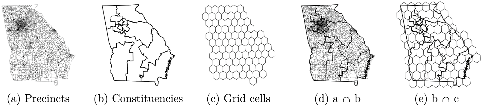
Figure 1 Spatial data layers (U.S. state of Georgia).
Precincts report to constituencies during the administration of elections, so units in Figure 1a should be fully nested within and smaller than those in Figure 1b. The intersection in Figure 1d confirms that every precinct falls inside a larger constituency, and—except for small border misalignments on the Atlantic coast—the transformation does not split precincts into multiple parts. If constituency IDs are available for precincts, a change of support from (a) to (b) could be reduced to calculating group sums, a straightforward procedure.
The hexagonal grid in (c) presents more difficulty. The grid cells were drawn independently of the other two layers, and are not nested. A transformation from (b) to (c) requires splitting constituencies across multiple grid cells, and vice versa. The overlay in Figure 1e suggests that cells are smaller than most, but not all, constituencies (e.g., Atlanta metro area). Changes of support to and from (c) therefore require complex spatial operations, accounting for differences in scale and misalignment of boundaries.
While visual assessments of nesting and scale can be informative, they introduce subjectivity and are often infeasible. Small geometric differences are difficult to detect visually, and partial degrees of nesting are hard to characterize consistently. Visual inspections are also slow and not scalable for batch processing, which requires automated subroutines.
We thus propose two nonparametric measures of relative nesting and scale. Let $\mathcal {G}_S$
be a set of source polygons, indexed
$\mathcal {G}_S$
be a set of source polygons, indexed $i=1,\dots ,N_S$
, and let
$i=1,\dots ,N_S$
, and let $\mathcal {G}_D$
be a set of destination polygons, indexed
$\mathcal {G}_D$
be a set of destination polygons, indexed $j=1,\dots ,N_D$
. Let
$j=1,\dots ,N_D$
. Let $\mathcal {G}_{S\cap D}$
be the intersection of these polygons, indexed
$\mathcal {G}_{S\cap D}$
be the intersection of these polygons, indexed ${i\cap j}=1,\dots ,N_{S\cap D} : N_{S\cap D}\geq \max (N_S,N_D)$
. Let
${i\cap j}=1,\dots ,N_{S\cap D} : N_{S\cap D}\geq \max (N_S,N_D)$
. Let $a_i$
be the area of source polygon i, let
$a_i$
be the area of source polygon i, let $a_j$
be the area of destination polygon j, and let
$a_j$
be the area of destination polygon j, and let $a_{i\cap j}$
be the area of
$a_{i\cap j}$
be the area of ${i\cap j} : a_{i\cap j}\leq \min (a_i,a_j)$
.Footnote
3
Let
${i\cap j} : a_{i\cap j}\leq \min (a_i,a_j)$
.Footnote
3
Let $M_{S\cap D}$
be an
$M_{S\cap D}$
be an $N_{S\cap D}\times 3$
matrix of indices mapping each intersection
$N_{S\cap D}\times 3$
matrix of indices mapping each intersection $i\cap j$
to its parent polygons i and j.
$i\cap j$
to its parent polygons i and j. $M_{i\cap D}$
is a subset of this matrix, indexing the
$M_{i\cap D}$
is a subset of this matrix, indexing the $N_{i\cap D}$
intersections of polygon i (see Section A2 of the Supplementary Material for examples). Let
$N_{i\cap D}$
intersections of polygon i (see Section A2 of the Supplementary Material for examples). Let $1(\cdot )$
be a Boolean operator, equal to 1 if “
$1(\cdot )$
be a Boolean operator, equal to 1 if “ $\cdot $
” is true.
$\cdot $
” is true.
Our first measure—relative nesting ( $RN$
)—captures how closely source and destination boundaries align, and whether one set fits neatly into the other:
$RN$
)—captures how closely source and destination boundaries align, and whether one set fits neatly into the other:
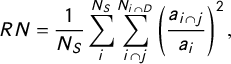 $$ \begin{align} RN = \frac{1}{N_S}\sum_{i}^{N_S} \sum_{i\cap j}^{N_{i\cap D}}\left(\frac{a_{i\cap j}}{a_i} \right)^2, \end{align} $$
which reflects the share of source units that are not split across destination units. Values of 1 indicate full nesting (no source units are split across multiple destination units), and a theoretical lower limit of 0 indicates no nesting (every source unit is split across many destination units). $RN$
has similarities with the Herfindahl–Hirschman Index (Hirschman Reference Hirschman1945) and the Gibbs–Martin index of diversification (Gibbs and Martin Reference Gibbs and Martin1962), which the electoral redistricting literature has used to assess whether “communities of interest” remain intact under alternative district maps (Chen Reference Chen2010). A value of
$RN$
has similarities with the Herfindahl–Hirschman Index (Hirschman Reference Hirschman1945) and the Gibbs–Martin index of diversification (Gibbs and Martin Reference Gibbs and Martin1962), which the electoral redistricting literature has used to assess whether “communities of interest” remain intact under alternative district maps (Chen Reference Chen2010). A value of $RN=1$
, for example, corresponds to redistricting plans in which every source unit is assigned to exactly one destination unit (e.g., “Constraint 1” in Cho and Liu Reference Cho and Liu2016).
$RN=1$
, for example, corresponds to redistricting plans in which every source unit is assigned to exactly one destination unit (e.g., “Constraint 1” in Cho and Liu Reference Cho and Liu2016).
The second measure—relative scale ( $RS$
)—captures whether a CoS task is generally one of aggregation or disaggregation:
$RS$
)—captures whether a CoS task is generally one of aggregation or disaggregation:
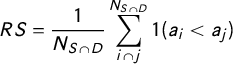 $$ \begin{align} RS = \frac{1}{N_{S\cap D}}\sum_{{i\cap j}}^{N_{S\cap D}}1(a_i<a_j) \end{align} $$
which is the share of intersections in which source units are smaller than destination units. Its range is 0 to 1, where 1 indicates pure aggregation (all source units are smaller than intersecting destination units) and 0 indicates no aggregation (all source units are at least as large as destination units). Values between 0 and 1 indicate a hybrid (i.e., some source units are smaller, others are larger than destination units).
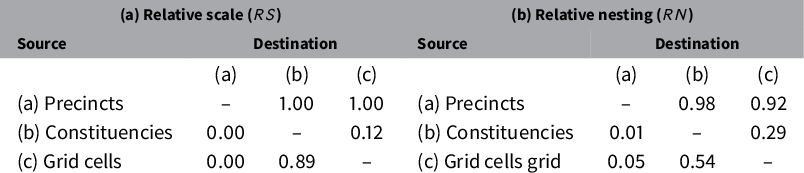
Table 1 reports pairwise $RN$
and
$RN$
and $RS$
measures for the polygons in Figure 1, with source units in rows and destination units in columns. The table confirms that precincts are always smaller (
$RS$
measures for the polygons in Figure 1, with source units in rows and destination units in columns. The table confirms that precincts are always smaller ( $RS=1$
) and almost fully nested within constituencies (
$RS=1$
) and almost fully nested within constituencies ( $RN=0.98$
), with the small difference likely due to measurement error. Precincts are also smaller than (
$RN=0.98$
), with the small difference likely due to measurement error. Precincts are also smaller than ( $RS=1$
) and mostly nested within grid cells (
$RS=1$
) and mostly nested within grid cells ( $RN=0.92$
). At the opposite extreme, obtaining precinct-level estimates from constituencies or grid cells would entail disaggregation (
$RN=0.92$
). At the opposite extreme, obtaining precinct-level estimates from constituencies or grid cells would entail disaggregation ( $RS=0$
) into non-nested units (
$RS=0$
) into non-nested units ( $0.01\leq RN \leq 0.05$
). Other pairings show intermediate values: hybrids of aggregation and disaggregation, where changes of support require splitting many polygons.
$0.01\leq RN \leq 0.05$
). Other pairings show intermediate values: hybrids of aggregation and disaggregation, where changes of support require splitting many polygons.
Table 1 Relative scale and nesting of polygons in Figure 1.
Before proceeding, let’s briefly consider how $RN$
and
$RN$
and $RS$
relate to each other, with more details in the Supplementary Material. Note, first, the two measures are not symmetric (i.e.,
$RS$
relate to each other, with more details in the Supplementary Material. Note, first, the two measures are not symmetric (i.e., $RS_{S,D}\neq 1- RS_{D,S}$
,
$RS_{S,D}\neq 1- RS_{D,S}$
, $RN_{S,D}\neq 1-RN_{D,S}$
), except in special cases where the outer boundaries of
$RN_{S,D}\neq 1-RN_{D,S}$
), except in special cases where the outer boundaries of $\mathcal {G}_S$
and
$\mathcal {G}_S$
and $\mathcal {G}_D$
perfectly align, with no “underlapping” areas as in Figure 1e. Section A2 of the Supplementary Material considers extensions of these measures, including symmetrical versions of
$\mathcal {G}_D$
perfectly align, with no “underlapping” areas as in Figure 1e. Section A2 of the Supplementary Material considers extensions of these measures, including symmetrical versions of $RS$
and
$RS$
and $RN$
, conditional metrics defined for subsets of units, measures of spatial overlap, and metrics that require no area calculations at all.
$RN$
, conditional metrics defined for subsets of units, measures of spatial overlap, and metrics that require no area calculations at all.
Second, as Table 1 suggests (and Section A2 of the Supplementary Material shows), the two measures are positively correlated. Relatively smaller units mostly nest within larger units. Yet because $RN$
is more sensitive to small differences in shape, area, and orientation, unlike
$RN$
is more sensitive to small differences in shape, area, and orientation, unlike $RS$
, it rarely reaches its limits of 1 or 0. Even pure aggregation (e.g., precinct-to-grid,
$RS$
, it rarely reaches its limits of 1 or 0. Even pure aggregation (e.g., precinct-to-grid, $RS=1$
) may involve integrating units that are technically not fully nested (
$RS=1$
) may involve integrating units that are technically not fully nested ( $RN=0.92$
). One barrier to reaching
$RN=0.92$
). One barrier to reaching $RN=1$
is that polygon intersections often result in small-area “slivers” due to minor border misalignments, but these can be easily excluded from calculation.Footnote
4
$RN=1$
is that polygon intersections often result in small-area “slivers” due to minor border misalignments, but these can be easily excluded from calculation.Footnote
4 $RN$
and
$RN$
and $RS$
can diverge, within a limited range, like in the precinct-to-grid example in Table 1. As Section A3 of the Supplementary Material shows using randomly generated maps, such divergence reflects the fact that the distributions of
$RS$
can diverge, within a limited range, like in the precinct-to-grid example in Table 1. As Section A3 of the Supplementary Material shows using randomly generated maps, such divergence reflects the fact that the distributions of $RN$
and
$RN$
and $RS$
have different shapes:
$RS$
have different shapes: $RS$
is bimodal, with peaks around
$RS$
is bimodal, with peaks around $RS=0$
and
$RS=0$
and $RS=1$
, while
$RS=1$
, while $RN$
is more normally distributed, with a mode around
$RN$
is more normally distributed, with a mode around $RN=0.5$
. The relationship between the two measures resembles a logistic curve, where numerical differences are largest in the tails and smallest in the middle. Differences between the measures tend to be numerically small. We observe no cases, for instance, where
$RN=0.5$
. The relationship between the two measures resembles a logistic curve, where numerical differences are largest in the tails and smallest in the middle. Differences between the measures tend to be numerically small. We observe no cases, for instance, where $RS>0.5$
and
$RS>0.5$
and $RN<0.5$
(or vice versa) for the same destination and source units.
$RN<0.5$
(or vice versa) for the same destination and source units.
2 How Nesting and Scale Affect Transformation Quality
How do the accuracy and bias of transformed values vary with relative nesting and scale? We evaluated the performance of several CoS algorithms in two applications: (1) transformations of electoral data across the polygons in Figure 1, and (2) a Monte Carlo study of CoS operations across randomly generated synthetic polygons. A comprehensive review of CoS methods, their assumptions and comparative advantages, is beyond the scope of this paper (see summary in Section A4 of the Supplementary Material). Instead, we focus on how relative scale and nesting affect the reliability of spatial transformations in general, holding one’s choice of CoS algorithm constant. Specifically, we compare transformed values in destination units to their “true” values across multiple CoS operations.
Let K be a set of CoS algorithms. Each algorithm, indexed $k\in \{1,\dots ,K\}$
, specifies a transformation
$k\in \{1,\dots ,K\}$
, specifies a transformation $f_k(\cdot )$
between source units
$f_k(\cdot )$
between source units $\mathcal {G}_S$
and destination units
$\mathcal {G}_S$
and destination units $\mathcal {G}_D$
. These transformations range from relatively simple operations that require no data beyond two sets of geometries, to more complex operations that incorporate information from covariates. Let
$\mathcal {G}_D$
. These transformations range from relatively simple operations that require no data beyond two sets of geometries, to more complex operations that incorporate information from covariates. Let $\mathbf {x}_{\mathcal {G}S}$
be an
$\mathbf {x}_{\mathcal {G}S}$
be an $N_{S}\times 1$
vector of observed values in source units
$N_{S}\times 1$
vector of observed values in source units $\mathcal {G}_S$
, and let
$\mathcal {G}_S$
, and let $\mathbf {x}_{\mathcal {G}D}$
be the
$\mathbf {x}_{\mathcal {G}D}$
be the $N_{D}\times 1$
vector of “true” values in destination units
$N_{D}\times 1$
vector of “true” values in destination units $\mathcal {G}_D$
. Let
$\mathcal {G}_D$
. Let $\widehat {\mathbf {x}_{\mathcal {G}D}}^{(k)}=f_k(\mathbf {x}_{\mathcal {G}S})$
be a vector of estimated values for
$\widehat {\mathbf {x}_{\mathcal {G}D}}^{(k)}=f_k(\mathbf {x}_{\mathcal {G}S})$
be a vector of estimated values for $\mathbf {x}_{\mathcal {G}D}$
, calculated using CoS algorithm k. These transformed values are typically point estimates, although some methods provide uncertainty measures.
$\mathbf {x}_{\mathcal {G}D}$
, calculated using CoS algorithm k. These transformed values are typically point estimates, although some methods provide uncertainty measures.
Consider the following CoS algorithms:
-
• Simple overlay. This method requires no re-weighting or geostatistical modeling, and is standard for the aggregation of event data. For each destination polygon, it identifies source features that overlap with it (polygons) or fall within it (points and polygon centroids), and computes statistics (e.g., sum and mean) for those features. If a source polygon overlaps with multiple destination polygons, it is assigned to the destination unit with the largest areal overlap. Advantages: speed, ease of implementation. Disadvantages: generates missing values, particularly if $N_S \ll N_D$
.
$N_S \ll N_D$
. -
• Area weighted interpolation. This is a default CoS method in many commercial and open-source GIS. It intersects source and destination polygons, calculates area weights for each intersection, and computes area-weighted statistics (i.e., weighted mean and sum). It can also handle point-to-polygon transformations through an intermediate tessellation step (Section A4 of the Supplementary Material). Advantages: no missing values, no ancillary data needed. Disadvantages: assumes uniform distribution in source polygons.
-
• Population weighted interpolation. This method extends area-weighting by utilizing ancillary data on population or any other covariate. It intersects the three layers (source, destination, and population), assigns weights to each intersection, and computes population-weighted statistics. Advantages: softens the uniformity assumption. Disadvantages: performance depends on quality and relevance of ancillary data.Footnote 5
-
• TPRS-Forest. This method uses a nonparametric function of geographic coordinates (thin-plate regression spline [TPRS]) to estimate a spatial trend, capturing systematic variation or heterogeneity (Davidson Reference Davidson2022b). It uses a Random Forest to model spatial noise, reflecting random, non-systematic variation. For each destination unit, it calculates a linear combination of trend and noise. Advantages: needs no ancillary data, provides estimates of uncertainty. Disadvantages: computationally costly.
-
• TPRS-Area weights. This is a hybrid of TPRS-Forest and areal interpolation. It decomposes source values into a non-stationary geographic trend using TPRS, and performs areal weighting on the spatial residuals from the smooth functional output (Davidson Reference Davidson2022a). Advantages: provides estimates of uncertainty for area weighting; can optionally incorporate ancillary data. Disadvantages: computationally costly.
-
• Ordinary (block) kriging. This model-based approach is widely used as a solution to the CoS problem in the natural and environmental sciences (Gotway and Young Reference Gotway and Young2007). It uses a variogram model to specify the degree to which nearby locations have similar values, and interpolates values of a random field at unobserved locations (or blocks representing destination polygons) by using data from observed locations. Advantages: provides estimates of uncertainty. Disadvantages: can generate overly smooth estimates, sensitive to variogram model selection, assumes stationarity.
-
• Universal (block) kriging. This extends ordinary kriging by using ancillary information. It interpolates values of a random field at unobserved locations (or blocks), using data on the outcome of interest from observed locations and covariates (e.g., population) at both sets of locations. Advantages: relaxes stationarity assumption. Disadvantages: ancillary data may not adequately capture local spatial variation.
-
• Rasterization. This is a “naive” benchmark against which to compare methods. It converts source polygons to raster (i.e., two-dimensional array of pixels), and summarizes the values of pixels that fall within each destination polygon. Advantages: no modeling, re-weighting or ancillary data. Disadvantages: assumes uniformity.

We employ two variants of the first three methods, using (a) polygon source geometries, and (b) points corresponding to source polygon centroids. These approaches represent different use cases: a “data-rich” scenario where full source geometries are available, and a “data-poor” scenario with a single address or coordinate pair. We also implement two variants of TPRS-Forest: (a) spatial trend only, and (b) spatial trend plus residuals.
We use three diagnostic measures: (1) root mean squared error, $\sqrt {\sum _j \frac {1}{N_D} (x_{j\mathcal {G}D} - \widehat {x_{j\mathcal {G}D}})^2}$
, (2) Spearman’s rank correlation for
$\sqrt {\sum _j \frac {1}{N_D} (x_{j\mathcal {G}D} - \widehat {x_{j\mathcal {G}D}})^2}$
, (2) Spearman’s rank correlation for $\mathbf {x}_{\mathcal {G}D}$
and
$\mathbf {x}_{\mathcal {G}D}$
and $\widehat {\mathbf {x}_{\mathcal {G}D}}$
, and (3) estimation bias,
$\widehat {\mathbf {x}_{\mathcal {G}D}}$
, and (3) estimation bias, $ E[\widehat {\beta }_{(\widehat {\mathbf {x}_{\mathcal {G}D}})}]-\beta _{(\mathbf {x}_{\mathcal {G}D})}$
, from an OLS regression of a synthetic variable
$ E[\widehat {\beta }_{(\widehat {\mathbf {x}_{\mathcal {G}D}})}]-\beta _{(\mathbf {x}_{\mathcal {G}D})}$
, from an OLS regression of a synthetic variable $\mathbf {y}$
(see below) on transformed values
$\mathbf {y}$
(see below) on transformed values $\hat {\mathbf {x}}$
. The first two diagnostics capture how closely the numerical values of the transformed variable align with true values, and the direction of association. The third captures the downstream impact of the CoS operation for model-based inference. For measures 1 and 3, values closer to zero are preferred. For measure 2, values closer to one are preferred.
$\hat {\mathbf {x}}$
. The first two diagnostics capture how closely the numerical values of the transformed variable align with true values, and the direction of association. The third captures the downstream impact of the CoS operation for model-based inference. For measures 1 and 3, values closer to zero are preferred. For measure 2, values closer to one are preferred.
2.1 Illustration: Changing the Geographic Support of Electoral Data
Our first illustration transforms electoral data across the polygons in Figure 1. We demonstrate generalizability through a parallel analysis of Swedish electoral data (Section A5 of the Supplementary Material).Footnote 6
The variable we transformed was Top-2 Competitiveness, scaled from 0 (least competitive) to 1 (most competitive):
 $$ \begin{align}\hspace{-40pt} \text{Top-2 Competitiveness}&=1-\text{winning party vote share margin} \qquad\qquad\qquad\qquad\qquad\end{align} $$
 $$ \begin{align}\hspace{30pt} &=\frac{\text{valid votes}-(\text{votes for winner}-\text{votes for runner-up})}{\text{valid votes}}. \end{align} $$
We obtained “true” values of competitiveness for precincts (Figure 1a) and constituencies (Figure 1b) from official election results, measuring party vote counts and votes received by all parties on the ballot (Kollman et al. Reference Kollman, Hicken, Caramani, Backer and Lublin2022). For grid cells (Figure 1c), we constructed aggregates of valid votes and their party breakdown from precinct-level results.
Our analysis did not seek to transform Top-2 Competitiveness directly from source to destination units. Rather, we transformed the three constitutive variables in Equation (4)—valid votes, and votes for the top-2 finishers—and reconstructed the variable after the CoS. In Section A6 of the Supplementary Material, we compare our results against those from direct transformation.
Because the purpose of much applied research is not univariate spatial transformation, but multivariate analysis (e.g., effect of $\mathbf {x}$
on
$\mathbf {x}$
on $\mathbf {y}$
), we created a synthetic variable,
$\mathbf {y}$
), we created a synthetic variable, $y_i=\alpha + \beta x_i + \epsilon _i$
, where
$y_i=\alpha + \beta x_i + \epsilon _i$
, where $x_i$
is Top-2 Competitiveness in unit i,
$x_i$
is Top-2 Competitiveness in unit i, $\alpha =1$
,
$\alpha =1$
, $\beta =2.5$
, and
$\beta =2.5$
, and $\epsilon \sim N(0,1)$
. We assess how changes of support affect the estimation of regression coefficients, in situations where the “true” value of that coefficient (
$\epsilon \sim N(0,1)$
. We assess how changes of support affect the estimation of regression coefficients, in situations where the “true” value of that coefficient ( $\beta =2.5$
) is known.
$\beta =2.5$
) is known.
Figure 2 shows transformed values of Top-2 Competitiveness ( $\widehat {\mathbf {x}_{\mathcal {G}D}}^{(k)}$
) alongside true values in destination units (
$\widehat {\mathbf {x}_{\mathcal {G}D}}^{(k)}$
) alongside true values in destination units ( $\mathbf {x}_{\mathcal {G}D}$
), where darker areas are more competitive. Figure 2a reports the results of precinct-to-constituency transformations (corresponding to “
$\mathbf {x}_{\mathcal {G}D}$
), where darker areas are more competitive. Figure 2a reports the results of precinct-to-constituency transformations (corresponding to “ $a \cap b$
” in Figure 1d). Figure 2b reports constituency-to-grid transformations (“
$a \cap b$
” in Figure 1d). Figure 2b reports constituency-to-grid transformations (“ $b \cap c$
” in Figure 1e). Of these two, the first set of transformations (where
$b \cap c$
” in Figure 1e). Of these two, the first set of transformations (where $RN=0.98$
,
$RN=0.98$
, $RS=1$
) more closely resembles true values than the second set (
$RS=1$
) more closely resembles true values than the second set ( $RN=0.29$
,
$RN=0.29$
, $RS=0.12$
), with fewer missing values and implausibly smooth or uniform predictions.
$RS=0.12$
), with fewer missing values and implausibly smooth or uniform predictions.
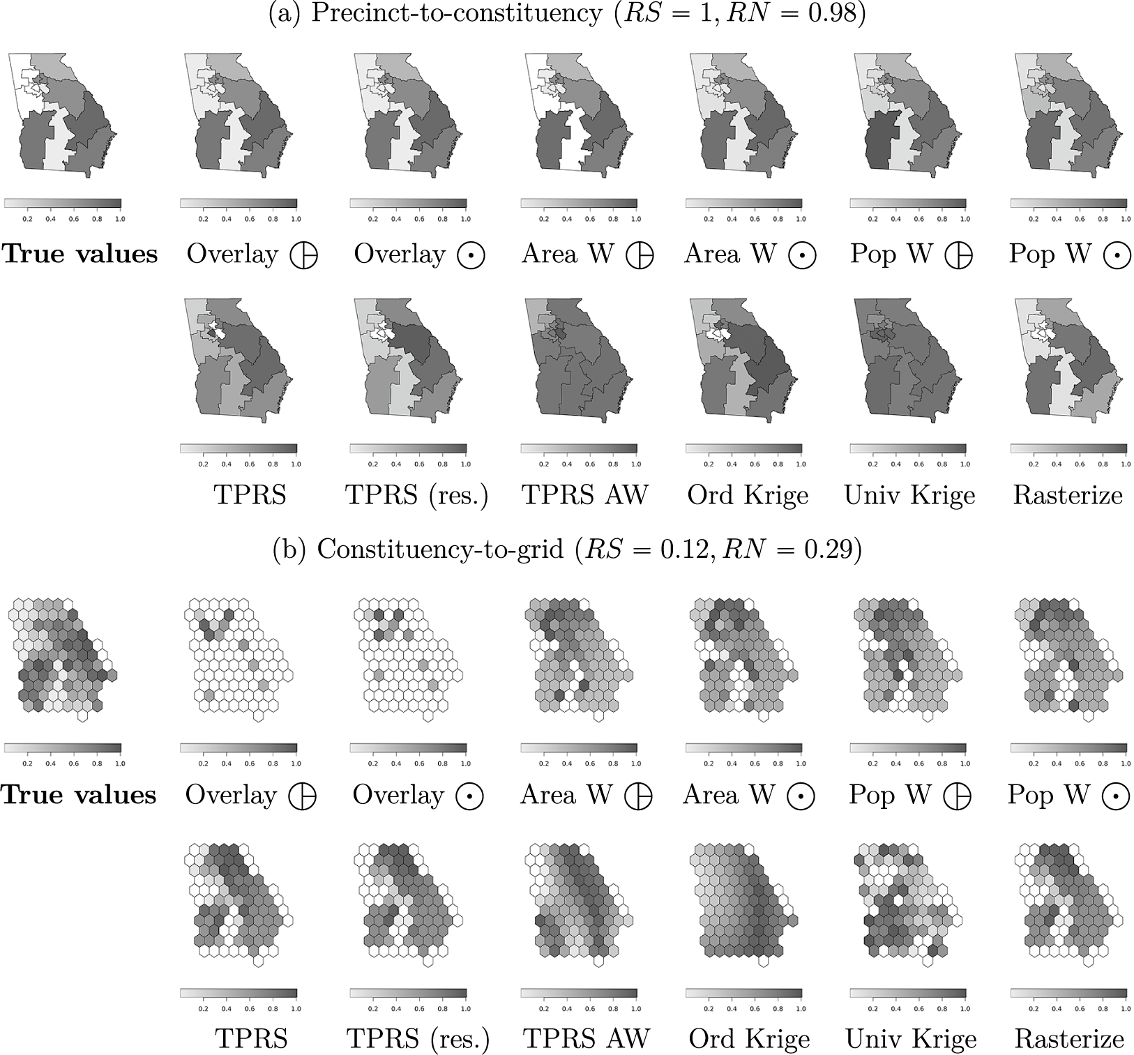
Figure 2 Output from change-of-support operations (Georgia).
![]() : source features are polygons.
: source features are polygons. $\bigodot $
: source features are polygon centroids.
$\bigodot $
: source features are polygon centroids.
Figure 3 reports fit diagnostics for the full set of CoS transformations across spatial units in Georgia (vertical axes), as a function of the transformations’ relative nesting and scale (horizontal axes). Each point corresponds the quality of fit for a separate CoS algorithm. The curves represent fitted values from a linear regression of each diagnostic on source-to-destination $RN$
and
$RN$
and $RS$
coefficients. Gray regions are 95% confidence intervals.
$RS$
coefficients. Gray regions are 95% confidence intervals.
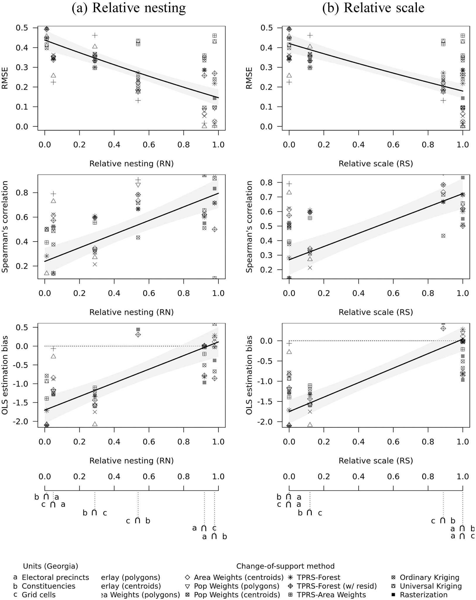
Figure 3 Relative nesting, scale and transformations of election data (Georgia).
The results confirm that the accuracy of CoS transformations increase in $RN$
and
$RN$
and $RS$
. RMSE is lower, correlation is higher, and OLS estimation bias is closer to 0 where source units are relatively smaller (Figure 3a) and more fully nested (Figure 3b). OLS bias is negative (i.e., attenuation) when
$RS$
. RMSE is lower, correlation is higher, and OLS estimation bias is closer to 0 where source units are relatively smaller (Figure 3a) and more fully nested (Figure 3b). OLS bias is negative (i.e., attenuation) when $RN$
and
$RN$
and $RS$
are small and shrinks toward 0 as they increase.
$RS$
are small and shrinks toward 0 as they increase.
Our analysis also reveals substantial differences in relative performance of CoS algorithms. Overall, simpler methods like overlays and areal interpolation produce more reliable results. For example, median RMSE—across all levels of $RN$
and
$RN$
and $RS$
—was 0.22 or lower for both types of simple overlays, compared to 0.43 for universal kriging. Median correlation for simple overlays was 0.85 or higher, compared to 0.12 for universal kriging. Simple overlays also returned the smallest OLS bias, with a median of
$RS$
—was 0.22 or lower for both types of simple overlays, compared to 0.43 for universal kriging. Median correlation for simple overlays was 0.85 or higher, compared to 0.12 for universal kriging. Simple overlays also returned the smallest OLS bias, with a median of $-0.15$
, compared to a quite severe underestimation of OLS coefficients for universal kriging (
$-0.15$
, compared to a quite severe underestimation of OLS coefficients for universal kriging ( $-2.4$
). Similar patterns emerge in our analysis of Swedish electoral data (Section A5 of the Supplementary Material).
$-2.4$
). Similar patterns emerge in our analysis of Swedish electoral data (Section A5 of the Supplementary Material).
Because the Top-2 Competitiveness variable is a function of other variables, we considered how transformation quality changes when we transform this variable directly versus reconstructing it from transformed components. The comparative advantages of these approaches depend on the relative nesting and scale of source and destination units: indirect transformations perform better when $RN$
and
$RN$
and $RS$
are closer to 1, direct transformations are preferable as
$RS$
are closer to 1, direct transformations are preferable as $RN$
and
$RN$
and $RS$
approach 0 (Section A6 of the Supplementary Material).
$RS$
approach 0 (Section A6 of the Supplementary Material).
2.2 Illustration: Monte Carlo Study with Synthetic Polygons
To generalize, we performed Monte Carlo simulations with artificial boundaries and variables on a rectangular surface. This analysis compares fit diagnostics from the same CoS algorithms, over a broader set of transformations covering the full range of $RN$
and
$RN$
and $RS$
.
$RS$
.
We consider two use cases. First, we change the geographic support of an extensive variable, like population size or number of crimes. Extensive variables depend on the area and scale of spatial measurement: if areas are split or combined, their values must be split or combined accordingly, such that the sum of the values in destination units equals the total in source units (i.e., satisfying the pycnophylactic, or mass-preserving, property). Second, we change the support of an intensive variable, like temperature or elevation. Intensive variables do not depend on the size of spatial units; quantities of interest in destination units are typically weighted means. Two or more extensive variables can combine to create a new intensive variable, like population density or electoral competitiveness. In Section A6 of the Supplementary Material, we consider the merits of (re-)constructing these variables before versus after a CoS.
While real-world data rarely conform to a known distribution, we designed the simulated geographic patterns to mimic the types of clustering and heterogeneity that are common in data on political violence and elections (see examples in Section A7 of the Supplementary Material).
At each iteration, our simulations executed these steps:
-
1. Draw random source (
$\mathcal {G}_S$
) and destination (
$\mathcal {G}_D$
) polygons. Within a rectangular bounding box
$\mathcal {B}$
, we sampled a random set of
$N_S$
points and created
$N_S$
tessellated polygons, such that for any polygon
$l_i \in \{1,\dots ,N_S\}$
corresponding to point
$i \in \{1,\dots ,N_S\}$
, all points inside
$l_i$
were closer to i than to any other point
$-i$
. We did the same for
$N_D$
destination polygons. The relative number of source-to-destination polygons (
$N_S$
:
$N_D$
) ranged from 10:200 to 200:10. Figure 4a shows one realization of
$\mathcal {G}_S,\mathcal {G}_D$
, with
$N_S=200,N_D=10$
.Figure 4 Examples of spatial data layers used in Monte Carlo study. Dotted lines are source units (
$\mathcal {G}_S$
), solid lines are destination units (
$\mathcal {G}_D$
). -
2. Assign “true” values of a random variable X to units in
$\mathcal {G}_S$
and
$\mathcal {G}_D$
. For extensive variables, we simulated values from an inhomogeneous Poisson point process (PPP). For intensive variables, we simulated values from a mean-zero Gaussian random field (GRF), implemented with the sequential simulation algorithm (Goovaerts Reference Goovaerts1997).Footnote
7
Figure 4b,c illustrates examples of each. In both cases, while we sought to imitate the spatially autocorrelated distribution of real-world social data, we also simulated spatially random values as benchmarks (see Section A7 of the Supplementary Material).Footnote
8
As before, we also created a synthetic variable
$Y=\alpha + X\beta + \epsilon $
, with
$\alpha =1$
,
$\beta =2.5$
,
$\epsilon \sim N(0,1)$
. -
3. Change the geographic support of X from
$\mathcal {G}_S$
to
$\mathcal {G}_D$
, using the CoS algorithms listed above. We then compared transformed values
$\widehat {x_{\mathcal {G}D}}$
to the assigned “true” values
$x_{\mathcal {G}D}$
, and calculated the same summary diagnostics as before, adding a normalized RMSE
$\left ({\sqrt {\sum _j \frac {1}{N_{\mathcal {G}D}} (x_{j\mathcal {G}D} - \widehat {x_{j\mathcal {G}D}})^2}}/{\left (\max (x_{\mathcal {G}D})-\min (x_{\mathcal {G}D})\right )}\right )$
for extensive variables.


We ran this simulation for randomly generated polygons with $N_S \in [10,\dots ,200]$
and
$N_S \in [10,\dots ,200]$
and $N_D \in [10,\dots ,200]$
, covering cases from aggregation (
$N_D \in [10,\dots ,200]$
, covering cases from aggregation ( $N_S=200,N_D=10$
) to disaggregation (
$N_S=200,N_D=10$
) to disaggregation ( $N_S=10,N_D=200$
). We repeated the process 10 times, with different random seeds.
$N_S=10,N_D=200$
). We repeated the process 10 times, with different random seeds.
To facilitate inferences about the relationship between nesting and the diagnostic measures, we estimated semi-parametric regressions of the form:
 $$ \begin{align} M_{km}&=f(RN_{km})+\text{Method}_k+\epsilon_{km}, \end{align} $$
where k indexes CoS algorithms, and m indexes simulations. $M_{km}$
is a diagnostic measure for CoS operation
$M_{km}$
is a diagnostic measure for CoS operation $km$
(i.e., [N]RMSE, correlation, OLS bias),
$km$
(i.e., [N]RMSE, correlation, OLS bias), $f(RN_{km})$
is a cubic spline of
$f(RN_{km})$
is a cubic spline of $RN$
(or
$RN$
(or $RS$
), Method
$RS$
), Method $_k$
is a fixed effect for each CoS algorithm, and
$_k$
is a fixed effect for each CoS algorithm, and $\epsilon _{km}$
is an i.i.d. error term. This specification restricts inferences to the effects of nesting and scale within groups of similar operations, adjusting for baseline differences in performance across algorithms.
$\epsilon _{km}$
is an i.i.d. error term. This specification restricts inferences to the effects of nesting and scale within groups of similar operations, adjusting for baseline differences in performance across algorithms.
Figure 5 reports predicted values of [N]RMSE, Spearman’s correlation, and OLS bias across all methods at different levels of $RN$
, for both (a) extensive and (b) intensive variables. Section A8 of the Supplementary Material reports results for the
$RN$
, for both (a) extensive and (b) intensive variables. Section A8 of the Supplementary Material reports results for the $RS$
coefficient, which generally align with these. As source units become more nested and relatively smaller, [N]RMSE and OLS bias trend toward 0, while correlation approaches 1. The primary difference between extensive and intensive variables is in the estimation of OLS coefficients. For extensive variables, we see attenuation bias, which becomes less severe as
$RS$
coefficient, which generally align with these. As source units become more nested and relatively smaller, [N]RMSE and OLS bias trend toward 0, while correlation approaches 1. The primary difference between extensive and intensive variables is in the estimation of OLS coefficients. For extensive variables, we see attenuation bias, which becomes less severe as $RN$
approaches 1. For intensive variables, we see attenuation bias as
$RN$
approaches 1. For intensive variables, we see attenuation bias as $RN$
approaches 1, but inflation bias as
$RN$
approaches 1, but inflation bias as $RN$
approaches 0.
$RN$
approaches 0.
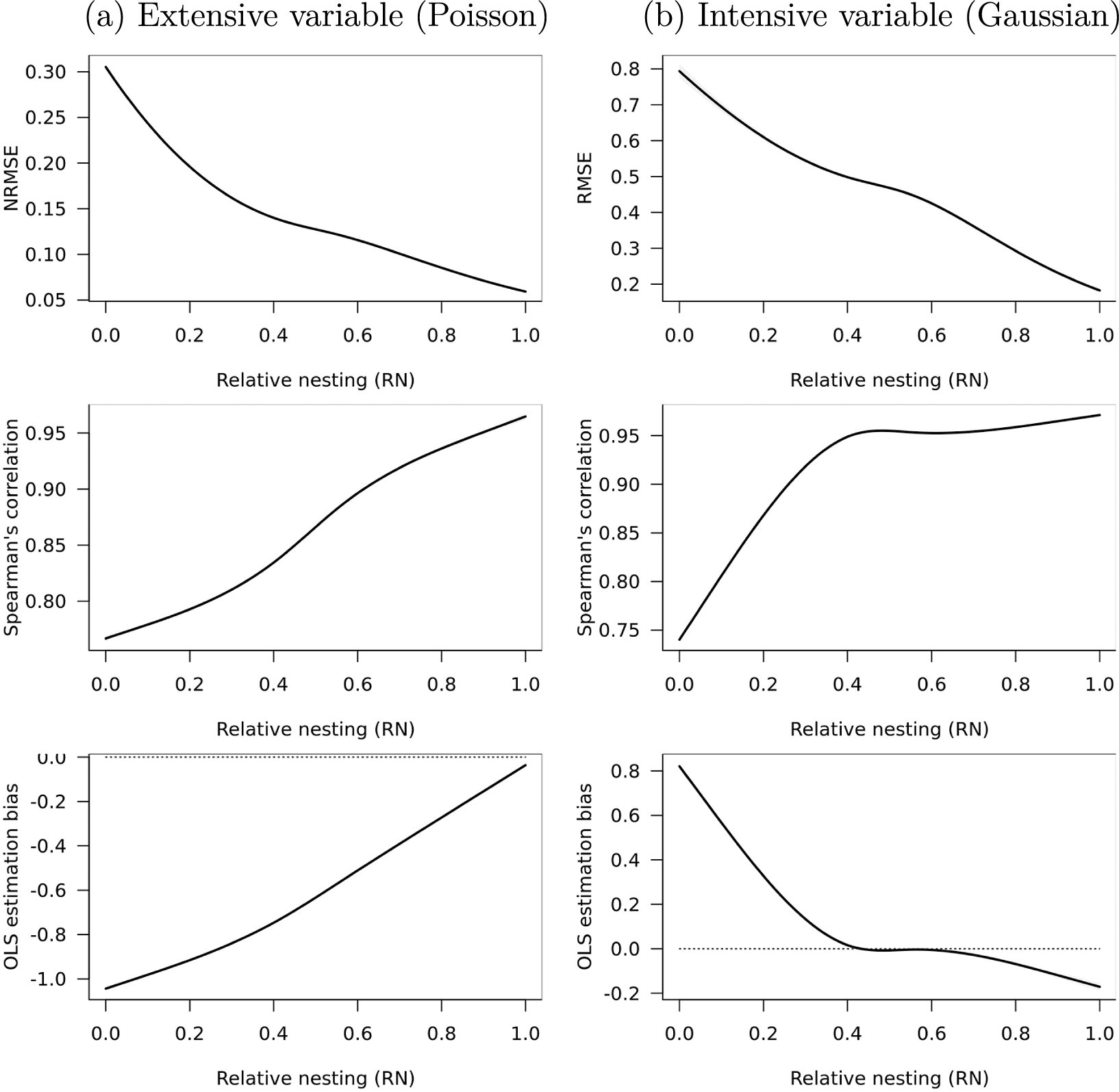
Figure 5 Relative nesting and transformations of synthetic data.
Figure 6 shows the Monte Carlo results by CoS algorithm, for (a) extensive and (b) intensive variables. In each matrix, the first, left-most column reports average statistics for each algorithm, pooled over all values of $RN$
. The remaining columns report average statistics in the bottom decile of
$RN$
. The remaining columns report average statistics in the bottom decile of $RN$
(0%–10%), the middle decile (45%–55%), and the top decile (90%–100%). The bottom row presents median statistics across algorithms. Darker colors represent better-fitting transformations (i.e., closer to 0 for [N]RMSE and bias; closer to 1 for correlation).
$RN$
(0%–10%), the middle decile (45%–55%), and the top decile (90%–100%). The bottom row presents median statistics across algorithms. Darker colors represent better-fitting transformations (i.e., closer to 0 for [N]RMSE and bias; closer to 1 for correlation).
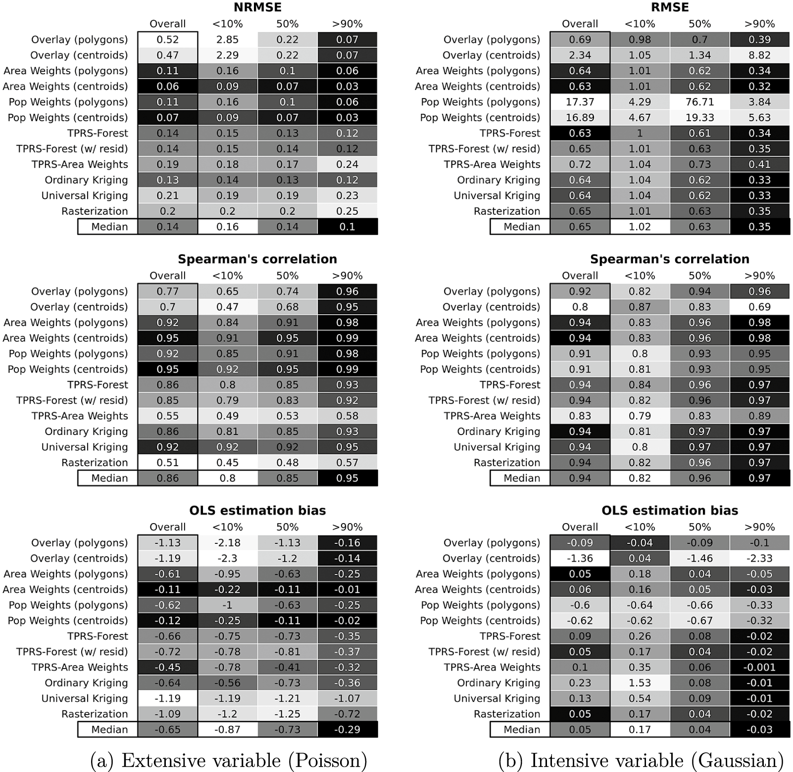
Figure 6 Transformation quality at different percentiles of relative nesting.
First, the relative performance of all CoS algorithms depends, strongly, on $RN$
(and
$RN$
(and $RS$
, see Section A8 of the Supplementary Material). In most cases, the largest improvements in performance occur between the lowest and middling ranges. Where values of
$RS$
, see Section A8 of the Supplementary Material). In most cases, the largest improvements in performance occur between the lowest and middling ranges. Where values of $RN$
are low (bottom 10%), most algorithms fare poorly. Performance improves as
$RN$
are low (bottom 10%), most algorithms fare poorly. Performance improves as $RN$
increases, especially in the first half of the range. For example, median RMSE (intensive variables) is 1.02 for CoS operations with low
$RN$
increases, especially in the first half of the range. For example, median RMSE (intensive variables) is 1.02 for CoS operations with low $RN$
, 0.63 for intermediate values, and 0.35 for the top decile. Most algorithms will perform better even at middling levels of
$RN$
, 0.63 for intermediate values, and 0.35 for the top decile. Most algorithms will perform better even at middling levels of $RN$
—0.4 and up—than at lower levels.
$RN$
—0.4 and up—than at lower levels.
Second, while no CoS algorithm clearly stands out, some perform consistently worse than others. For example, population weighting offers no discernible advantages in transforming intensive variables (but seemingly plenty of disadvantages) relative to simple area weighting. Ancillary data from covariates, these results suggest, do not always improve transformation quality. Centroid-based simple overlays also fare poorly throughout.
Third, some CoS algorithms are more sensitive to variation in $RN$
than others. For example, simple overlays produce credible results for extensive variables when
$RN$
than others. For example, simple overlays produce credible results for extensive variables when $RN$
is high, while areal and population weighting results are more stable.
$RN$
is high, while areal and population weighting results are more stable.
Are $RN$
and
$RN$
and $RS$
redundant? After we condition on
$RS$
redundant? After we condition on $RN$
, for example, does
$RN$
, for example, does $RS$
add any explanatory value in characterizing the quality of CoS operations (i.e., measurement error and bias of transformed values)? As we show in Section A3 of the Supplementary Material,
$RS$
add any explanatory value in characterizing the quality of CoS operations (i.e., measurement error and bias of transformed values)? As we show in Section A3 of the Supplementary Material, $RN$
is more strongly predictive of transformation quality than
$RN$
is more strongly predictive of transformation quality than $RS$
when considering the two metrics separately. But
$RS$
when considering the two metrics separately. But $RS$
is not redundant; including information about both
$RS$
is not redundant; including information about both $RN$
and
$RN$
and $RS$
accounts for more variation in transformation quality than does information about
$RS$
accounts for more variation in transformation quality than does information about $RN$
alone.Footnote
9
$RN$
alone.Footnote
9
In Section A3 of the Supplementary Material, we consider how divergence between $RN$
and
$RN$
and $RS$
affects the relative performance of CoS methods. Not much, we conclude. The absolute proximity of
$RS$
affects the relative performance of CoS methods. Not much, we conclude. The absolute proximity of $RS$
and
$RS$
and $RN$
to 0 or 1 is far more predictive of transformation quality than their divergence.
$RN$
to 0 or 1 is far more predictive of transformation quality than their divergence.
Our simulations confirm that patterns from our analysis of election data—higher $RN$
and
$RN$
and $RS$
are better—hold in more general sets of cases. These include changes of support between units of highly variable sizes and degrees of nesting, and transformations of variables with different properties and distributional assumptions.
$RS$
are better—hold in more general sets of cases. These include changes of support between units of highly variable sizes and degrees of nesting, and transformations of variables with different properties and distributional assumptions.
3 What Is to Be Done?
Changes of support with medium to high relative nesting and scale tend to produce higher quality transformations, in terms of lower error rates, higher rank correlation, and lower OLS estimation bias. These patterns persist across CoS algorithms, in applications involving both extensive and intensive variables. While some CoS methods do perform better than others in specific contexts, no method stands out unconditionally dominating the rest. We were unable to find a “winner” in our comparison of a dozen algorithms, using data from elections and Monte Carlo simulations that mimic different geospatial patterns.
What does this mean for analysts performing CoS operations? We recommend reporting $RN$
and
$RN$
and $RS$
coefficients for all CoS operations as ex ante measures of transformation complexity. This requires no data beyond the geometries of source and destination polygons, and enables readers to assess risks of poor inference: the higher the numbers, the more reliable the potential results—and midrange numbers typically give one far more confidence than lower numbers. Also, for face validity of transformed values, good practice is to map the new distribution, and visually inspect it for strange discontinuities, missingness, “unnatural” smoothness or uniformity, and other obvious errors (as in Figure 2). We urge researchers to implement sensitivity analyses with alternative CoS methods, to show that their results do not rest on assumptions of particular algorithms.
$RS$
coefficients for all CoS operations as ex ante measures of transformation complexity. This requires no data beyond the geometries of source and destination polygons, and enables readers to assess risks of poor inference: the higher the numbers, the more reliable the potential results—and midrange numbers typically give one far more confidence than lower numbers. Also, for face validity of transformed values, good practice is to map the new distribution, and visually inspect it for strange discontinuities, missingness, “unnatural” smoothness or uniformity, and other obvious errors (as in Figure 2). We urge researchers to implement sensitivity analyses with alternative CoS methods, to show that their results do not rest on assumptions of particular algorithms.
Beyond this, advice depends on the availability of two types of “ground truth” data relevant to changes of support: atomic-level information on the distribution of variables being transformed (e.g., precinct-level vote tallies and locations of individual events), and information on the proper assignment of units (e.g., cross-unit IDs).
If researchers have access to irreducibly lowest-level (ILL) data—in addition to aggregate values in source units—we recommend using ILL data to validate spatial transformations directly. Examples of ILL data include precinct-level votes, point coordinates of events, ultimate sampling units, individual-level (micro) data, and other information that cannot be disaggregated further. With such data, one can implement CoS methods as in the above analyses, and select the algorithm that yields the smallest errors and highest correlation with aggregates of true values in destination units. Alternatively, researchers may simply use the ILL data as their source features, since they are likely to have high $RN$
and
$RN$
and $RS$
scores with destination units.
$RS$
scores with destination units.
If IDs for destination polygons are available for source units and $RN$
and
$RN$
and $RS$
are sufficiently high, then spatial transformations via CoS algorithms may be unnecessary. For each destination polygon, one needs only to identify the source features that share the common identifier (e.g., county name and state abbreviation), and compute group statistics for those features. The ID variable must exist, however, and provide a one-to-one or many-to-one mapping. A source feature assigned to more than one destination unit needs additional assumptions about how source values are (re-)distributed.
$RS$
are sufficiently high, then spatial transformations via CoS algorithms may be unnecessary. For each destination polygon, one needs only to identify the source features that share the common identifier (e.g., county name and state abbreviation), and compute group statistics for those features. The ID variable must exist, however, and provide a one-to-one or many-to-one mapping. A source feature assigned to more than one destination unit needs additional assumptions about how source values are (re-)distributed.
What if there are no lower-level data for validation, and no common IDs for unit assignment? Our general advice—reporting $RN$
and
$RN$
and $RS$
, visually inspecting the results, and performing sensitivity analyses—still holds. Yet the third of these steps has pitfalls. Since we cannot know which set of estimates is closest to true values, rerunning one’s analysis with alternative CoS algorithms can create temptations either to be biased and choose the numbers one likes best, or to give equal weight to all algorithms, including some that could be wildly off the mark.
$RS$
, visually inspecting the results, and performing sensitivity analyses—still holds. Yet the third of these steps has pitfalls. Since we cannot know which set of estimates is closest to true values, rerunning one’s analysis with alternative CoS algorithms can create temptations either to be biased and choose the numbers one likes best, or to give equal weight to all algorithms, including some that could be wildly off the mark.
While cross-validation without ground truth data is a difficult topic that is beyond the scope of this article, we briefly illustrate one potential path in Section A9 of the Supplementary Material. Specifically, one can report the results of multiple CoS methods, along with a measure of how divergent each set of results is from the others, using outlier detection tests. As an analogy, this is like using multiple, imperfect instruments to detect the amount of oil underground. We may never know the true amount. But learning (for instance) that only one of the instruments has detected the presence of hydrocarbons is useful, both in the search for oil—that instrument might get it right—but also in evaluating the outlier instrument for future efforts. We caution that no set of results should be included or excluded from analysis solely on the basis of an outlier detection test. It is possible for an outlier to be more accurate than the average, and alternatively, an algorithm giving results close to average may be quite inaccurate. Yet if a CoS method frequently gives output that differs systematically from other CoS methods, further investigation may be warranted into the deviant algorithm. At the very least, this would help contextualize one’s results.
To provide researchers with routines, documentation, and source code to implement these and other procedures with their own data, we developed an open-source software package (SUNGEO), available through the Comprehensive R Archive Network and GitHub. It includes functions to calculate $RN$
,
$RN$
, $RS$
and related metrics, as well as functions to execute—and compare—most of the CoS methods discussed in this article. These tools should enable researchers to explore options, elucidate the consequences of choices, and design CoS strategies to meet their needs.
$RS$
and related metrics, as well as functions to execute—and compare—most of the CoS methods discussed in this article. These tools should enable researchers to explore options, elucidate the consequences of choices, and design CoS strategies to meet their needs.
4 Conclusion
When integrating data across spatial units, seemingly benign measurement decisions can produce nontrivial consequences. The accuracy of spatial transformations depends on the relative nesting and scale of source and destination units. We introduced two simple, nonparametric measures that assess the extent to which units are nested and the range from aggregation to disaggregation. We have shown that the two measures are predictive of the quality of spatial transformations, with higher values of $RN$
and
$RN$
and $RS$
associated with lower error rates, higher correlation between estimated and true values, and less severe OLS estimation bias. These measures can serve as ex ante indicators of spatial transformation complexity and error-proneness, even in the absence of “ground truth” data for validation. We also provide open-source software to help researchers implement these procedures.
$RS$
associated with lower error rates, higher correlation between estimated and true values, and less severe OLS estimation bias. These measures can serve as ex ante indicators of spatial transformation complexity and error-proneness, even in the absence of “ground truth” data for validation. We also provide open-source software to help researchers implement these procedures.
Because changes of support entail information loss, the consequences of these problems will depend in part on whether one uses spatially transformed estimates for description or inference. Researchers have leeway when using transformed measures for mapping and visualization, so long as these transformed estimates correlate with the (unobserved) ground truth. The situations become more precarious when using interpolated measures for inference. Both Type II and Type I errors are possible. In the case of extensive variables, transformations with lower $RN$
and
$RN$
and $RS$
scores generally result in the under-estimation of OLS coefficients, increasing the chances of false negatives. Yet there are also cases where estimation bias is in the opposite direction (e.g., intensive variables with low
$RS$
scores generally result in the under-estimation of OLS coefficients, increasing the chances of false negatives. Yet there are also cases where estimation bias is in the opposite direction (e.g., intensive variables with low $RN$
and
$RN$
and $RS$
), increasing the chances of false positives. More research is needed on these situations.
$RS$
), increasing the chances of false positives. More research is needed on these situations.
We reiterate that CoS problems are ignored at the peril of accurate inference, and there is no silver bullet. Researchers should document their measurement choices. This includes reporting relative nesting and scale, checking the face validity of the output, and avoiding reliance on a single CoS algorithm. We encourage future research to explore new methods for integrating spatially misaligned data.
Acknowledgments
For helpful comments, we thank Wendy Tam Cho, Karsten Donnay, Rob Franzese, Jeff Gill, Max Goplerud, Andrew Linke, Walter Mebane, Kevin Quinn, Jonathan Rodden, Melissa Rogers, Yuki Shiraito, and three anonymous reviewers.
Supplementary Material
For supplementary material accompanying this paper, please visit https://doi.org/10.1017/pan.2023.5.
Data Availability Statement
Replication data and code have been published in Code Ocean, a computational reproducibility platform that enables users to run the code, and can be viewed interactively at codeocean.com/capsule/7981862/tree (Zhukov et al. Reference Zhukov, Byers, Davidson and Kollman2023a). A preservation copy of the same code and data can also be accessed via Dataverse at doi.org/10.7910/DVN/TOSX7N (Zhukov et al. Reference Zhukov, Byers, Davidson and Kollman2023b). The R package is available at cran.r-project.org/package=SUNGEO and github.com/zhukovyuri/SUNGEO.
Funding
Funding for this research was provided by an NSF RIDIR grant under award number SES-1925693.


 Open access