


Radiocarbon in dissolved inorganic carbon (DI14C) in seawater has long been recognized as an important tracer for studying ocean processes. DII4C is reported as Δ14C in per mille units as defined in Stuiver and Polach (Reference Stuiver and Polach1977). The earliest ocean measurements from the 1950s focused on deep ocean circulation rates (Bien et al. Reference Bien, Rakestraw and Suess1960; Broecker et al. Reference Broecker, Gerard, Ewing and Heezen1960). Early studies of the surface ocean were thought to be complicated by the known lack of steady-state in the atmospheric radiocarbon content due to the atmospheric 14C decrease since the Industrial Revolution (the Suess effect: e.g., Suess Reference Suess1953; Keeling Reference Keeling1979; Stuiver and Quay Reference Stuiver and Quay1981) and the sharp increase in 14C since the atmospheric weapons tests in the 1950s and 1960s (the bomb spike, e.g., Rafter Reference Rafter1965; Nydal Reference Nydal1968). At the time, it was understood how useful the bomb spike would be for studying air-sea gas exchange in the future (Bien et al. Reference Bien, Rakestraw and Suess1960) and as a global carbon cycle tracer experiment. Reidar Nydal championed the collection and analysis of surface ocean radiocarbon starting in the mid-1960s (Nydal et al. Reference Nydal1984), amassing a data set of over 500 analyses between 1966 and 1981. The early work demonstrated the power of DI14C to study ocean processes but was limited in scope because of the challenges of collecting the samples and making the measurements.
Until the advent of accelerator mass spectrometry (AMS) in the early 1990s, up to 250 L of seawater was required to obtain a precise radiocarbon measurement, i.e., a measurement with a precision of ± 2–4‰ in the deep ocean. Two samplers in use until the early to mid 1990s were Gerard barrels (Bien et al. Reference Bien, Rakestraw and Suess1960; Broecker et al. Reference Broecker, Gerard, Ewing and Heezen1960) and keg samplers (Young et al. Reference Young, Buddemeier and Fairhall1969) (Figure 1). The former has a capacity of ∼250 L, and the latter, repurposed beer kegs, had a capacity of up to ∼60 L. Gerard samples were acidified on the ship using 40 mL of concentrated H2SO4 and sparged for about four hours (depending on sample temperature) using CO2-free air or N2. Extracted CO2 was precipitated as either BaCO3, SrCO3, or dissolved in KOH or NaOH and transferred to shore-based laboratories for analysis and counting using specialized gas proportional (Östlund et al. Reference Östlund, Bowman and Rusnak1962) or liquid scintillation (Tamers Reference Tamers1960) counters. The amount of time required to collect the Gerard samples coupled with the lengthy shipboard extraction procedure severely limited the numbers of samples that could be collected and analyzed. Regardless, the GEOSECS data collected during the 1970s provide an extraordinarily valuable baseline for the more extensive subsequent surveys.
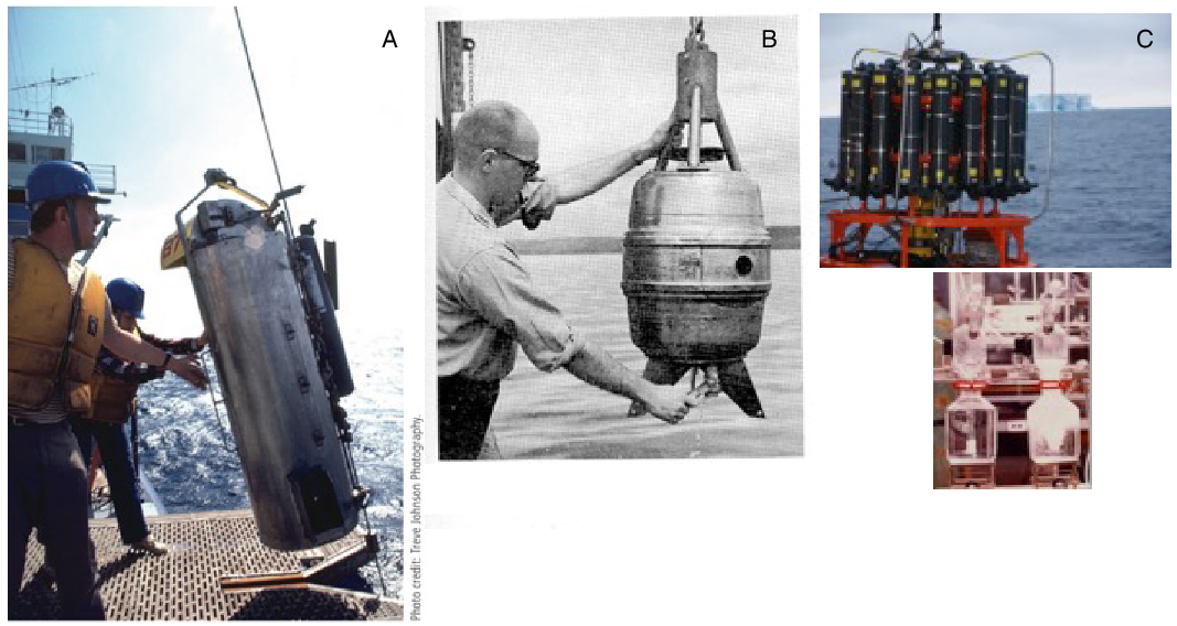
Figure 1 Samplers used to collect water for radiocarbon analysis: A. Gerard barrel, B. Keg sampler, C. Niskin bottles. A and B use the entire volume of water for the analysis while only 500 mL are collected from the Niskin bottle.
The handling and difficulty of ensuring good recoveries also made it challenging to use these samples for DI13C measurements of adequate precision and accuracy to be oceanographically meaningful; therefore, separate samples were used for these analyses (Kroopnik Reference Kroopnick1985). The reduction in sample size afforded by AMS (from 250 L to 0.5 L) made it possible to collect samples at sea, preserve them with HgCl2, and ship them back to laboratories for analysis. Until recently, the preferred extraction method for both DI14C and DI13C has been sparging with CO2-free gases, usually N2 (Bard Reference Bard, Arnold, Maurice and Duplessy1987; Quay Reference Quay, Tilbrook and Wong1992; McNichol Reference McNichol, Jones, Hutton, Gagnon and Key1994). Newer methods include headspace analysis (Gao et al. Reference Gao, Xu, Zhou, Pack, Griffin, Santos, Southon and Liu2014) and membrane transfer techniques (Gospodinova et al. Reference Gospodinova, McNichol, Gagnon and Walter2016). Once the gas has been extracted, standard techniques are used for the analysis of radiocarbon (Vogel et al. Reference Vogel, Southon and Nelson1987; Roberts et al. Reference Roberts, Burton, Elder, Longworth, McIntyre, von Reden, Han, Rosenheim, Jenkins, Galutschek and McNichol2010; Longworth et al. Reference Longworth, von Reden, Long and Roberts2015). Shipboard-based analysis using non AMS techniques to measure radiocarbon at sea, at least for waters containing bomb-produced carbon, allowing researchers to walk off the ship with data, will bring radiocarbon on par with chlorofluorocarbons (CFCs) for wider utilization within the oceanographic community. Much progress is needed but cavity-ring down systems similar to those in use for DI13C (Su et al. Reference Su, Cai, Hussain, Brodeur, Chen and Huang2019) hold promise for the future (Galli et al. Reference Galli, Bartalini, Ballerini, Barucci, Cancio, De Pas, Giusfredi, Mazzotti, Akikusa and De Natale2016; Fleisher et al. Reference Fleisher, Long, Liu, Gameson and Hodges2017).
The first global sampling program to include DI14C was the Geochemical Ocean Sections Study (GEOSECS) in the mid-1970s (Östlund and Stuiver Reference Östlund and Stuiver1980; Stuiver and Östlund Reference Stuiver and Östlund1980, Reference Stuiver and Östlund1983). A major force in the measurement of DI14C in the GEOSECS program and many of the programs that followed was Wally Broecker. As noted in a memoir (Broecker Reference Broecker2012), his interest was piqued during a conversation with Henry Stommel. Specifically, Broecker recalled, “Toward the end of the 1960s, two unique opportunities arose which led me to temporarily abandon my desire to plunge ever more deeply into paleoclimate. One was the creation by the National Science Foundation of an initiative called IDOE (International Decade of Ocean Exploration) and the other was an invitation to participate in a limnological research program being launched in Canada. In 1968, during a visit to Woods Hole, Henry Stommel, a legendary figure in physical oceanography, took me aside and said, ‘Wally, you guys measure radiocarbon here and there in the ocean, but if we are to properly use the results to pin down the rates of transport, we need a systematic survey along transects from one end of the ocean to the other.’ I asked, ‘how many stations along each transect and how many depths at each station?’ He replied, ‘50 stations and 20 depths.’ ”
The GEOSECS goal was to increase the general knowledge of ocean geochemistry and to estimate the deep-ocean transport rates. Sampling consisted of a single section along the center of each major ocean basin. The GEOSECS Program introduction states, “As man [sic] becomes increasingly aware of the ocean as a source of food, a disposal area for nuclear and industrial waste products, a strategic realm for national security and a controlling factor in the earth’s climatic regime, he also recognizes how very little he knows about the sea.” Data from the early programs up through the original World Ocean Circulation Experiment (WOCE) occupations are stored in easily accessible internet locations (e.g., CLIVAR and Carbon Hydrographic Data Office [CCHDO], National Centers for Environmental Information [NCEI], Ocean Carbon Data System [OCADS]) and summarized in the Global Ocean Data Analysis Project (GLODAP) database (Key et al. Reference Key, Kozyr, Sabine, Lee, Wanninkhof, Bullister, Feely, Millero, Mordy and Peng2004). Sample numbers cited here reflect those in GLODAPv2.2020 (Olsen et al. Reference Olsen, Lange, Key, Tanhua, Bittig, Kozyr, Álvarez, Azetsu-Scott, Becker and Brown2020) and include data reported through 2015 (mostly samples from the Climate Variability and Predictability [CLIVAR] and the Global Ocean Ship-Based Hydrographic Investigations Program [GO-SHIP] programs). During GEOSECS, 2218 DI14C values from 125 stations were reported. Subsequent large programs were the Transient Tracers in the Ocean (TTO, 1981–1983, 937 values from 101 stations; Brewer et al. Reference Brewer, Sarmiento and Smethie1985; Östlund and Rooth Reference Östlund and Rooth1990) and the South Atlantic Ventilation Experiment (SAVE, 1987–1989, 955 values from 77 stations) in the Atlantic Ocean, as well as the Indien Gaz Ocean (INDIGO, 1985–1987, 233 samples; Östlund and Grall Reference Östlund and Grall1991, 430 values from 20 stations) project in the Indian and Southern Oceans. The primary goal of these programs was to extend the two-dimensional description of the tracer distributions into three dimensions so that the properties could be mapped on density surfaces. Much of this earlier work used the fact that, in the 1960s and by GEOSECS in the 1970s, ocean DI14C was controlled by air-sea exchange and had not penetrated deeply enough to be a good tracer analog for the uptake of anthropogenic CO2.
During the 1990s the WOCE program was carried out “to survey the global distribution of ocean variables with a view to greatly improving estimates of the circulation of heat, water and chemicals around the world ocean, and their exchange with the atmosphere (Woods Reference Woods1985).” The advent of AMS greatly increased the number of radiocarbon samples that could be collected and measured (see below) and 17,676 samples were measured as part of this program. Because the highest precision was needed in the deep water and the AMS technique was new, large volume samples were collected in the deep waters and small volume samples were collected in the surface and thermocline waters. The United States WOCE program collected and analyzed the majority of these samples at a laboratory funded and built primarily for this program (Jones et al. Reference Jones, McNichol, von Reden and Schneider1990) referred to as the National Ocean Sciences Accelerator Mass Spectrometry Facility (NOSAMS). Other countries whose laboratories measured radiocarbon included Japan (primarily the Japanese Agency for Marine-Earth Science and Technology) and Germany. WOCE was followed by the CLIVAR programs in the first decade of the 2000s. These programs were designed to better understanding climate variability and predictability on seasonal to centennial time scales, identifying processes responsible for climate change, and developing predictive capabilities (http://www.clivar.org). The most recent program is GO-SHIP, a program that has a goal of providing the measurements needed to understand and document large-scale ocean water property distributions, their changes, and their drivers in a changing global environment (http://www.go-ship.org). As of 2015, CLIVAR, GO-SHIP, and other smaller programs have added 14,085 measurements to the global database.
Results from these programs and sample analyses have contributed greatly to our understanding of the oceans. DI14C is affected by biology and carbonate chemistry, but by normalizing to 13C and time, the biological effect is minimized. This allows 14C, reported as Δ14C (or strictly Δ as per Stuiver and Polach Reference Stuiver and Polach1977), to be used as a physical tracer for both anthropogenic carbon and as a water mass tracer to elucidate dynamics. Monitoring of the oceanic 14C transient in the upper ocean has provided important metrics of surface-to-deep exchange rates predicted by ocean models, and, specifically, deep water formation rates and processes in key locations where continued penetration of anthropogenic CO2 into the interior and abyssal ocean is occurring. Changes in ocean 14C can now be used to track the arrival of anthropogenic CO2 in the abyssal ocean (Graven et al. Reference Graven, Gruber, Key, Khatiwala and Giraud2012), where the DIC changes are still small (< 2 μmol kg-1) and difficult to detect using back-calculation approaches (e.g., ΔC* [Gruber et al. Reference Gruber, Sarmiento and Stocker1996] and variants thereof). The radiocarbon distribution and change have been used to study mixing, ventilation rates, rates of production of abyssal waters, shallow upwelling rates, and deep ocean residence times (Broecker et al. Reference Broecker, Peng and Stuiver1978, Reference Broecker, Peacock, Walker, Weiss, Fahrbach, Schroeder, Mikolajewicz, Heinze, Key, Peng and Rubin1998; Broecker Reference Broecker1979; Toggweiler and Samuels Reference Toggweiler and Samuels1993; Toggweiler and Key Reference Toggweiler and Key2001; Matsumoto and Key Reference Matsumoto, Sarmiento, Key, Aumont, Bullister, Caldeira, Campin, Doney, Drange and Dutay2004; Roussenov et al. Reference Roussenov, Williams, Follows and Key2004; Schlitzer Reference Schlitzer2007), deep ocean biogeochemistry and oxygen utilization rates (Broecker et al. Reference Broecker, Blanton, Smethie and Østlund1991; Key Reference Key2001; Keller et al. Reference Keller, Slater, Bender and Key2002; Sarmiento et al. Reference Sarmiento, Simeon, Gnanadesikan, Gruber, Key and Schlitzer2007), air-sea gas exchange (Broecker and Peng Reference Broecker and Peng1974; Wanninkhof Reference Wanninkhof1992; Sweeney et al. Reference Sweeney, Gloor, Jacobson, Key, McKinley, Sarmiento and Wanninkhof2007), thermocline ventilation rates (Gnanadesikan et al. Reference Gnanadesikan, Dunne, Key, Matsumoto, Sarmiento, Slater and Swathi2004), as a proxy for anthropogenic CO2 in the ocean (Broecker et al. Reference Broecker, Peng and Takahashi1980), to estimate deep water mass ages for anthropogenic CO2 uptake and carbon studies (Sabine et al. Reference Sabine, Key, Johnson, Millero, Sarmiento, Wallace and Winn1999, Reference Sabine, Key, Feely and Greely2002a, Reference Sabine, Feely, Key, Bullister, Millero, Lee, Peng, Tilbrook, Ono and Wong2002b, Reference Sabine, Bullister, Feely, Gruber, Key, Kozyr, Lee, Millero, Ono, Peng, Tillbrook, Wallace, Wanninkhof and Wong2004; Feely et al. Reference Feely, Sabine, Lee, Millero, Lamb, Greeley, Bullister, Key, Peng, Kozyr, Ono and Wong2002; Chung et al. Reference Chung, Lee, Feely, Sabine, Millero, Key and Wanninkhop2003, Reference Chung, Park, Lee, Key, Millero, Feely, Sabine and Falkowski2004; Lee et al. Reference Lee, Choi, Park, Wanninkhof, Peng, Key, Sabine, Feely, Bullister and Millero2003), and to evaluate ocean general circulation model (OGCM) performance (Maier-Reimer and Hasselmann Reference Maier-Reimer and Hasselmann1987; Toggweiler et al. Reference Toggweiler, Dixon and Bryan1989a, Reference Toggweiler, Dixon and Bryan1989b; Guilderson et al. Reference Guilderson, Caldeira and Duffy2000; Key Reference Key2001; Orr et al. Reference Orr, Maier-Reimer, Mikolajewicz, Monfray, Sarmiento, Toggweiler, Taylor, Palmer, Gruber and Sabine2001; Key et al. Reference Key, Kozyr, Sabine, Lee, Wanninkhof, Bullister, Feely, Millero, Mordy and Peng2004; Matsumoto et al. Reference Matsumoto, Sarmiento, Key, Aumont, Bullister, Caldeira, Campin, Doney, Drange and Dutay2004).
An elegant example of the power of 14C analyses is provided by Toggweiler et al. (Reference Toggweiler, Druffel, Key and Galbraith2019a, Reference Toggweiler, Druffel, Key and Galbraith2019b). Their 14C assessment combined surface water Δ14C data from biogenic carbonate archives, primarily reef-building corals, and DIC samples from the WOCE/CLIVAR programs to place a constraint on the volume of water upwelled in the major upwelling centers of the global ocean and to provide insights on the mechanism of upwelling and forcing. The regional (and when combined, global) upwelling indicated by the spatial range of upwelling induced surface water Δ14C deficits exceeds that which would be indicated by the surface wind (Ekman) forcing alone. In the Pacific, where the Δ14C deficit stretches across the basin, Ekman-based forcing indicates an upwelling volume of ∼2Sv off the coast of Peru and the Costa Rican Dome, whereas the Δ14C budget indicates more than 10Sv. Similar differences occur in the other major upwelling regions. The Δ14C surface deficit upwelling estimates are consistent with inverse modeling estimates in terms of the volume of water that upwells.
The inverse models, however, use large amounts of diapycnal mixing to transform relatively dense Antarctic Circumpolar Water (ACC) into lighter water. The newly formed “lighter” or less dense water can then be shunted to the surface by denser water pushing through the ACC into mode and interior water masses. In contrast, the Δ14C data imply nearly direct exposure of interior water via upwelling of mode and intermediate waters at the western basin margins. If upwelling is geographically limited to these upwelling sources, less diapycnal mixing is needed to transform interior and mode waters to waters that are more easily mixed into the surface. Toggweiler et al. posit that the additional volume, beyond that required by Ekman forcing, upwelled in these regional locations and required to balance the surface water DI14C distribution is a “push” associated with the global thermohaline circulation: i.e., the classic “conveyor belt” initially coined by Arnold Gordon and made famous by Wally Broecker. The reduced impact of diapycnal mixing will require improved physics in ocean models that predict anthropogenic CO2 uptake.
The Ocean Carbon Model Intercomparison Project (OCMIP) was one of the first major collaborative efforts between transient tracer experts and ocean modelers to explore DI14C in a coordinated, meaningful, and mechanistic way. The goal was to understand the processes that caused differences in model simulations, predictions and to improve model capabilities. Radiocarbon and CFC data were used as tracers. The OCMIP model predictions of the CFC distribution were much better than for DI14C. This is largely because the CFC distribution is strongly dependent on surface ocean temperature that the models reproduce reasonably well, although biases in mixed layer depth propagate into CFC inventory biases (e.g., Long et al. Reference Long, Lindsay, Peacock, Moore and Doney2013). Both natural and bomb radiocarbon provide model constraints not available from any other tracer. Figure 2 compares OCMIP results with WOCE 14C data from section P16 (Key et al. Reference Key, Quay, Jones, McNichol, Von Reden and Schneider1996; Stuiver et al. Reference Stuiver, Östlund, Key and Reimer1996). Although all of the models reproduce the general shape of the contours, the concentrations vary widely. The model physics required to reproduce the 14C distribution are much more difficult and involve the entire water column. Even cursory examination points out significant discrepancies in all model results, e.g., a too diffuse thermocline, and remarkable model to model differences. One conclusion was that some models could reasonably reproduce the sparse GEOSECS data, but none could adequately simulate the WOCE results (Orr et al. Reference Orr, Maier-Reimer, Mikolajewicz, Monfray, Sarmiento, Toggweiler, Taylor, Palmer, Gruber and Sabine2001): i.e., continued circulation and movement of Δ14C showed flaws in model dynamics and their predictive transport skill.

Figure 2 OCMIP-2 results. All of the model results and the data are colored and scaled identically and the portion of the section containing bomb radiocarbon has been masked.
In recent decades (post 1995), air-sea exchange exerts less influence on ocean DI14C because the air-sea 14C gradients are now very small. In some regions such as the equatorial Pacific the flux is likely from the ocean back into the atmosphere (Figure 3a). This means that, for samples collected since mid-WOCE, the dominant control on oceanic DI14C has been surface-to-deep exchange, similar to the situation for anthropogenic CO2 (Graven et al. Reference Graven, Gruber, Key, Khatiwala and Giraud2012). In fact, in recent decades anthropogenic CO2 uptake and oceanic 14C uptake are strongly correlated in ocean models (Figure 3b). After the formal portion of OCMIP, model-data Δ14C comparisons degenerated back to single model or at best two data-model comparisons (e.g., Galbraith et al. Reference Galbraith, Kwon, Gnanadesikan, Rodgers, Griffies, Bianchi, Sarmiento, Dunne, Simeon and Slater2011; Graven et al. Reference Graven, Gruber, Key, Khatiwala and Giraud2012), including eddy resolving models (e.g., Lachkar et al. Reference Lachkar, Orr, Dutay and Delecluse2007). OCMIP led to model specific developments and advancements. At Princeton, a series of sensitivity studies using a coarse model (Modular Ocean Model, or MOM) lead to the MOM model doing better at reproducing deep water radiocarbon in addition to a better understanding of thermocline ventilation processes (Gnanadesikan et al. Reference Gnanadesikan, Slater, Gruber and Sarmiento2002, Reference Gnanadesikan, Dunne, Key, Matsumoto, Sarmiento, Slater and Swathi2004; Galbraith et al. Reference Galbraith, Kwon, Gnanadesikan, Rodgers, Griffies, Bianchi, Sarmiento, Dunne, Simeon and Slater2011). Sensitivity experiments such as these and data-model comparisons (e.g., Guilderson et al. Reference Guilderson, Caldeira and Duffy2000) have shed light on the challenges of accurately modeling ocean dynamics in regions with significant vertical fluxes.
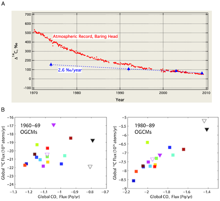
Figure 3 A. Surface ocean DI14C (blue diamonds) at 32°S in the Pacific at 4 time points compared to atmospheric record (red dots). B. Relationship between global ocean CO2 and 14C uptake in a collection of ocean models in the 1960s (left) and in the 1980s (right). (Figure adapted from Graven et al. Reference Graven, Gruber, Key, Khatiwala and Giraud2012.)
Largescale coupled models have improved through the application of subgrid scale parameterization that impacts horizontal movement and mixing. Yet, issues remain with the models’ representation of vertical dynamics as well as the incomplete understanding of the coupling with overlying wind-field and eddy-scale processes. This is slowly leading the modeling community away from “model democracy” where every model is equally viable, to focusing on models that achieve certain observation-based metrics better than others (e.g., Beadling et al. Reference Beadling, Russell, Stouffer, Mazloff, Talley, Goodman, Sallée, Hewitt, Hyder and Pandde2020). One metric that integrates atmosphere-ocean coupling, vertical dynamics, and the surface ocean’s radiative balance is the model sea surface temperature (SST) field and how big and where any model-data bias occurs. SST bias in the Geophysical Fluid Dynamics Laboratory (GFDL) CM2Mc Earth System model (Figure 4) is representative of many earth system and OGCMs used in CMIP (c.f., fig 1 in Wang et al. Reference Wang, Zhang, Lee, Wu and Mechoso2014). The general statements that model cloud biases and a bias in the position and/or intensity of major wind systems (e.g., the Southern Ocean westerlies and western boundary wind systems) impact the surface radiative budget and are thus the cause of the observed model-data SST bias, although accurate, do not quite capture model failures. A cloud-forced radiative imbalance leading to SST biases does not directly explain the models’ failures to accurately recreate the volume of water upwelling (and the Δ14C values and “regional deficits”) in these regions (c.f., Toggweiler et al. Reference Toggweiler, Druffel, Key and Galbraith2019a, Reference Toggweiler, Druffel, Key and Galbraith2019b). These regions are sources and sinks of nutrients and atmospheric CO2, and have large impacts on ocean biogeochemistry. Model reproduction of decadal change is notoriously more difficult than reproducing a single snapshot of property distributions. Continued data-model comparisons using radiocarbon can lead to insights into inaccuracies in how mesoscale eddies are treated in the models and their effect on mixing as well as understanding the transfer of properties such as energy from the surface to the deep ocean. Small changes in the parameterization of mesoscale eddies can have a large impact on climate sensitivity (Fox-Kemper et al. Reference Fox-Kemper, Adrocft, Böning, Chassignet, Curchitser, Danabasoglu, Eden, England, Gerdes and Greatbatch2019). Moving beyond “tuning exercises” the tracer data in the Repeat Hydrography Sections represent an opportunity to improve modeling of vertical dynamics and interior, deep circulation and, therefore, to increase models’ ability to predict the sources and sinks of nutrients and carbon in surface water.

Figure 4 SST error or bias in the GFDL CM2Mc Earth System model relative to observations (after Galbraith et al. Reference Galbraith, Kwon, Gnanadesikan, Rodgers, Griffies, Bianchi, Sarmiento, Dunne, Simeon and Slater2011). Similar biases in space and amplitude are observed in nearly all of the CMIP models (Wang et al. Reference Wang, Zhang, Lee, Wu and Mechoso2014). At the western boundaries, SST biases are accompanied by biases in upwelling volume. In the Southern Ocean the SST biases are accompanied by insensitivity of overturning rates with increased winds.
There is a recognition that the climate system has tipping or bifurcation points where the system can rapidly shift to an alternative state but will not return to the original state even when the forcing perturbation is removed (c.f., IPCC 2019). Acting much like a bath-tub drain, the Southern Ocean has been a significant modifier of anthropogenic atmospheric CO2 and heat: the formation of interior and deep waters removes atmospheric CO2 from the surface ocean (and thus from the atmosphere) and at the same time moves heat away from the surface (Purkey and Johnson Reference Purkey and Johnson2013; Johnson and Lyman Reference Johnson and Lyman2020). Largescale changes in the overlying wind (Ekman) forcing has the ability to alter the circulation in such a manner to decrease the uptake of heat and CO2. However, teasing out natural multi-decadal variability associated with the Southern Annular Mode and its teleconnection to the Pacific Decadal Oscillation from changes directly forced by anthropogenic-induced climate change will be difficult in this sparsely sampled, yet incredibly important region. The Southern Ocean Carbon and Climate Observations and Modeling Program (SOCCOM) is currently working to “unlock (sic) the mysteries of the Southern Ocean,” at least in the upper 2000 m. Flexibility in the funding model for the radiocarbon portion of GO-SHIP has allowed the collection of DI14C samples at selected SOCCOM float sites. The well-documented poleward movement and intensification of the southern hemisphere westerlies observed in 2000–2010s (e.g., Fyfe et al. Reference Fyfe, Saenko, Zickfeld, Eby and Weaver2007; Lin et al. Reference Lin, Zhai, Wang and Munday2018) have continued with an increase in the intensity of the 90th percentile winds (Young and Ribal Reference Young and Ribal2019). This change has the potential to erode surface waters thus exposing subsurface or interior water with higher concentrations of CO2. This will reduce the ability of these surface waters to take up anthropogenic CO2 (e.g., Gray et al. Reference Gray, Johnson, Bushinsky, Riser, Russell, Talley, Wanninkhof, Williams and Sarmiento2018 Keppler and Landschützer Reference Keppler and Landschuutzer2019). Will deeper mixing associated with the winds and reduced salinity due to Antarctic glacial ice melting increase the stability of the Southern Ocean to yield a “new” mode of Southern Ocean circulation (e.g., Bronselaer et al. Reference Bronselaer, Russell, Winton, Williams, Key, Dunne, Feely, Johnson and Sarmiento2020)? This could have grave implication for the climate system as a whole and for future climate change scenarios.
Radiocarbon has a large dynamic range in the ocean. It is one of tools the oceanographic and modeling communities have to monitor changes in the structure of the Southern Ocean. In particular, the vertical and horizontal gradients of Δ14C are sensitive to the competing effects of the air-sea 14C disequilibrium isotope flux and the exhumation of low-Δ14C interior water. Repeated meridional Southern Ocean sections frequent enough to distinguish sub-decadal variability associated with the Southern Annular Mode from secular changes across regions most important to upwelling, interior water formation, and air-sea CO2 exchange will be a powerful diagnostic of the state of the Southern Ocean and a necessary model benchmark to elucidate biases.
ACKNOWLEDGMENTS
The authors thank J. R. Toggweiler for helpful comments on versions of this paper. Authors received funding from the National Science Foundation OCE-85865400 (APM) and a Woods Hole Oceanographic Technical Staff Award (APM).


 Open access