


1 Introduction
Reactivity plays a major part in many areas of computing. For instance, it is an important feature in situated agent systems and it forms the foundation of many state transition systems. It also plays a part in constraint handling rules and abstract state machines and reactive programming in general (Mancarella et al. Reference Mancarella, Terreni, Sadri, Toni and Endriss2009; Kowalski and Sadri Reference Kowalski and Sadri1999; Costantini and Tocchio Reference Costantini and Tocchio2004; Alferes et al. Reference Alferes, Banti and Brogi2006; Rao Reference Rao2009; Frühwirth Reference Frühwirth1998; Gurevich Reference Gurevich2000a). Reactivity can take several different forms, such as event-condition-action rules, for instance in active databases, or condition-action rules, for example in production systems, or transition rules in abstract state machines (Zaniolo Reference Zaniolo2003; Lausen et al. Reference Lausen, Ludäscher and May1998; Fernandes et al. Reference Fernandes, Williams and Paton1997; Russell and Norvig Reference Russell and Norvig2003; Gurevich Reference Gurevich2000b). Reactivity is implicit in some systems, such as BDI agents, whereas in other systems it is explicit and core, for example Reaction RuleML and logic production system (LPS) (Rao and Georgeff Reference Rao and Georgeff1995; Paschke et al. Reference Paschke, Boley, Zhao, Teymourian and Athan2012; Kowalski and Sadri 2011; Reference Kowalski and Sadri2015). Consider, for example, an agent situated in an environment. The agent may have some initial goals towards which it may plan and execute actions. But, to be effective, it also needs to take account of the changes in its environment and react to them by setting itself new goals and adjusting its old goals and any already constructed (partial) plans. This is also in the spirit of (Teleo)reactive systems, which have the primary objective to increase the responsiveness and resilience of computer systems without the need for replanning (Clark Reference Clark2018; Clark and Robinson Reference Clark and Robinson2015; Nilsson Reference Nilsson1994; Sanchez et al. Reference Sanchez, Alvarez, Morales and Navarro2016).
ASP (Answer Set Programming) (Gebser et al. Reference Gebser, Kaminski, Kaufmann and Schaub2013; Brewka et al. Reference Brewka, Eiter and TruszczyŃski2011) is a paradigm of declarative programming, rooted in logic programming, that has gained popularity in recent years and has been applied in several interesting domains, such as planning, semantic web, computer-aided verification and health care (Erdem et al. Reference Erdem, Gelfond and Leone2016). Given a logic program, ASP computes its models, called answer sets, which can be considered solutions to the problem captured by the logic program.
In this work we show how reactivity can be incorporated within the ASP paradigm by adopting the notion of reactivity from another logic-based paradigm, KELPS (KErnel of LPS) (Kowalski and Sadri Reference Kowalski and Sadri2016). We call the resulting framework Reactive ASP. KELPS (and LPS) is based on abductive logic programming and combines reactive rules with logic programs, a database and a causal theory that specifies transitions between the states of the database. We chose KELPS as the basis for Reactive ASP for two reasons. Firstly, the logic-based syntax of KELPS and its notion of reactivity are, in our opinion, quite general and intuitive – for example they subsume both event-condition-action rules and condition-action rules. Secondly, KELPS provides a formal definition of reactivity which guided our design of Reactive ASP and its formal verification.
The operational semantics (OS) of KELPS is based on the cycle illustrated in Figure 1. Starting from an initial state (database), incoming external events and the framework’s own generated actions are assimilated and the state is updated, and reactive rules whose conditions have become true given the history of events and states so far are triggered. This results in new goals to satisfy, and their incremental partial solutions, in turn, result in more actions generated to be executed, thus iterating through the cycle. As well as an OS KELPS has a model-theoretic semantics, and KELPS computation is aimed at generating models for the reactive rules in dynamic environments. These models can be infinite.

Fig. 1. KELPS operational semantics cycle.
The paper makes several contributions:
-
It shows how to facilitate reactivity in ASP by first defining a variant of KELPS with a finite number of state changes in any model, called n-distant KELPS, and then giving a mapping from this n-distant KELPS to Reactive ASP. We prove that the mapping is sound and complete in the sense that, given any initial state and any ensuing sets of external events, the answer sets of the resulting Reactive ASP programs correspond exactly to the n-distant KELPS reactive models.
-
The mapping is then used to shed light on possible relationships and synergies between the two different paradigms. In particular, we show that it facilitates for free additional alternative control strategies and a prospective style of programming (Pereira and Lopes Reference Pereira and Lopes2009), which allows to consider future consequences of present decisions in order to choose what to do presently.
-
Furthermore, we propose an approach that combines features of KELPS with ASP into one unified architecture that enjoys the benefits of KELPS OS and its destructive updates of the state where no frame axiom reasoning is needed, together with the flexibility of ASP that allows prospective and preference reasoning.
Notions of reactivity have been considered in ASP in other work but these approaches are different from the form presented here. For example, in a tool for maritime traffic control, maritime explain how they used oclingo, a particular form of reactive ASP that handles external data, now superseded by clingo 4 (Gebser et al. Reference Gebser, Grote, Kaminski and Schaub2011), in order to handle histories efficiently inside the ASP system. Thus the work in generating answer sets at each time step is reduced by discarding information from previous time steps that is no longer useful. In ribeiro the notion of reactivity in ASP is used to mean efficiency in reasoning by partitioning the knowledge base so that reasoning is done only with the part relevant to the context, whereas Brewka, at the end of his paper (Brewka Reference Brewka2013), sketches a notion of reactivity closer to ours. He proposes as future work the use of rules that have “operational statements in their heads”, where these operations are “read off” from the generated answer sets and the program is modified accordingly. Recently, some applications using iclingo (an ASP system that incorporates incremental grounding) to simulate reactivity have been described in Recenticlingo.
The rest of the paper is structured as follows. Section 2 provides background on KELPS and ASP. Section 3 describes and exemplifies the mapping between the two, while Section 4 provides theoretical results. Section 5 discusses how Reactive ASP allows more complex control strategies and prospection. In Section 6 we then propose a hybrid of the two paradigms of KELPS and ASP that combines their advantages. We illustrate this hybrid system with examples and discuss two different ways of realising it. Section 7 reviews the mappings discussed earlier in the paper and provides further insights in the comparison of the incremental behaviour of KELPS and Reactive ASP. It then briefly introduces an alternative incremental mapping to ASP and its implementation in clingo 4 and gives a brief empirical evaluation of our approach (with more detail in Appendix B). It finally discusses related work by looking at other approaches to reactivity and prospection in logic programming. In Section 8 we discuss future work and conclude.
2 Background
This section introduces the KELPS framework and reviews relevant features of ASP.
2.1 KELPS
KELPS (Kowalski and Sadri Reference Kowalski and Sadri2016) is a logic-based state transition framework combining reactivity with a destructively updated database and a causal theory that has both an OS and a model-theoretic semantics. KELPS is a subset of the full LPS language (Kowalski and Sadri Reference Kowalski and Sadri2011). LPS has been implemented in Prolog, Java, Python and SWISH and has been used in currently ongoing industry-based applications in smart contracts and industry production control. The SWISH proptotype implementation of LPS (Wielemaker et al. Reference Wielemaker, Riguzzi, Kowalski, Lager, Sadri and Calejo2019) is downloadable and together with LPS examples can be found at http://lps.doc.ic.ac.uk.
2.1.1 The KELPS vocabulary
KELPS uses a first-order sorted language including a sort for linear and discrete time, in which the predicate symbols (and consequently atoms) of the language are partitioned into sets representing fluents, events, auxiliary predicates and meta-predicates. Fluent predicates are used to represent time-dependent facts in the KELPS state. In their timestamped form,
 $p(t_1,...,t_n, i)$
, their last argument
$p(t_1,...,t_n, i)$
, their last argument
 $i\geq 0$
represents the time of the state
$i\geq 0$
represents the time of the state
 $S_i$
to which the fluent belongs. The atom
$S_i$
to which the fluent belongs. The atom
 $p(t_1, ..., t_n)$
is called the unstamped fluent. Event predicates capture events, both observed external events and events generated by the framework itself (sometimes called actions to distinguish them). Events contribute to state transitions – that is, they map one state into a successor state. In their timestamped form,
$p(t_1, ..., t_n)$
is called the unstamped fluent. Event predicates capture events, both observed external events and events generated by the framework itself (sometimes called actions to distinguish them). Events contribute to state transitions – that is, they map one state into a successor state. In their timestamped form,
 $e(t_1,...,t_n, i)$
, their last argument
$e(t_1,...,t_n, i)$
, their last argument
 $i\geq 1$
represents the time of the (successor) state
$i\geq 1$
represents the time of the (successor) state
 $S_i$
and the event is said to take place in the transition between state
$S_i$
and the event is said to take place in the transition between state
 $S_{i-1}$
and
$S_{i-1}$
and
 $S_i$
. The event atom
$S_i$
. The event atom
 $e(t_1, ..., t_n)$
is called the unstamped event.
Footnote 1
Auxiliary predicates are of two kinds: (i) time-independent predicates (and corresponding atoms) do not include time parameters and represent properties that are not affected by events, for example, isa(book, item), denoting that book is an item; and (ii) temporal constraint predicates (and corresponding atoms) use only time parameters in arguments and express temporal constraints, including inequalities of the form
$e(t_1, ..., t_n)$
is called the unstamped event.
Footnote 1
Auxiliary predicates are of two kinds: (i) time-independent predicates (and corresponding atoms) do not include time parameters and represent properties that are not affected by events, for example, isa(book, item), denoting that book is an item; and (ii) temporal constraint predicates (and corresponding atoms) use only time parameters in arguments and express temporal constraints, including inequalities of the form
 $T1 < T2$
and
$T1 < T2$
and
 $T1 \leq T2$
between time points, and functional relationships among time points, such as max(T1,T2,T), denoting that T is the maximum of T1 and T2. The KELPS meta-predicates initiates(event, fluent) and terminates(event, fluent) express the fluents that are initiated and terminated by events. In general the first argument would be a set of events, to cater for cases where a set of events may have a different impact on state changes from the sum of the effects of each of the constituent events. In our mapping to ASP we define these meta-predicates for single events only. This caters for all cases where concurrent events are independent of each other, that is they do not affect the same fluent.
$T1 \leq T2$
between time points, and functional relationships among time points, such as max(T1,T2,T), denoting that T is the maximum of T1 and T2. The KELPS meta-predicates initiates(event, fluent) and terminates(event, fluent) express the fluents that are initiated and terminated by events. In general the first argument would be a set of events, to cater for cases where a set of events may have a different impact on state changes from the sum of the effects of each of the constituent events. In our mapping to ASP we define these meta-predicates for single events only. This caters for all cases where concurrent events are independent of each other, that is they do not affect the same fluent.
2.1.2 The KELPS framework
The KELPS framework is specified by a tuple
 $<\mathcal{R}$
,
$<\mathcal{R}$
,
 $\mathcal{C}$
,
$\mathcal{C}$
,
 $\mathcal{A}ux >$
consisting of a set
$\mathcal{A}ux >$
consisting of a set
 $\mathcal{R}$
of reactive rules, a causal theory
$\mathcal{R}$
of reactive rules, a causal theory
 $\mathcal{C}$
specifying pre-conditions and post-conditions of the events that cause state transitions, and a set
$\mathcal{C}$
specifying pre-conditions and post-conditions of the events that cause state transitions, and a set
 $\mathcal{A}ux$
of auxiliary ground atoms. A reactive rule has the logical form
$\mathcal{A}ux$
of auxiliary ground atoms. A reactive rule has the logical form
 \begin{equation}\forall \overline{X}[antecedent(\overline{X})\rightarrow \exists \overline{Y} consequent(\overline{X1},\overline{Y})]\end{equation}
in which the consequent is a disjunction
 $consequent_1 \lor \ldots \lor consequent_n $
, the antecedent and each
$consequent_1 \lor \ldots \lor consequent_n $
, the antecedent and each
 $consequent_{i} $
is a conjunction of conditions, where each condition is either a fluent literal, an event atom, or an auxiliary literal.
Footnote 2
In equation (1)
$consequent_{i} $
is a conjunction of conditions, where each condition is either a fluent literal, an event atom, or an auxiliary literal.
Footnote 2
In equation (1)
 $\overline{Y}$
is the set of all variables that occur only in
$\overline{Y}$
is the set of all variables that occur only in
 $consequent(\overline{X1}, \overline{Y})$
,
$consequent(\overline{X1}, \overline{Y})$
,
 $\overline{X}$
is the set of remaining variables in the rule and
$\overline{X}$
is the set of remaining variables in the rule and
 $\overline{X1} \subseteq \overline{X}.$
Footnote 3
Note that because of the restrictions of the quantification of variables in reactive rules we can omit the quantifier prefixes without ambiguity and write
$\overline{X1} \subseteq \overline{X}.$
Footnote 3
Note that because of the restrictions of the quantification of variables in reactive rules we can omit the quantifier prefixes without ambiguity and write
 $antecedent(\overline{X})\rightarrow consequent(\overline{X1},\overline{Y}) $
. All timestamps in consequent are equal to, or later than, all timestamps in antecedent.
$antecedent(\overline{X})\rightarrow consequent(\overline{X1},\overline{Y}) $
. All timestamps in consequent are equal to, or later than, all timestamps in antecedent.
For example, consider the following policy: If a customer (Cust) makes a request for an item (Item) at time T, then either the item is available and the agent allocates the item to the customer at some time
 $T_1$
later than T, and then processes the order, all to be done before 4 units of time after T, or the agent apologises about the item to the customer at 4 units of time after T. Moreover, if an item is allocated to a customer, there are fewer than 2 units of that item left afterwards and the item is not already on order, then the agent must order 20 units of it at the next time unit. This can be expressed as two reactive rules in KELPS:
$T_1$
later than T, and then processes the order, all to be done before 4 units of time after T, or the agent apologises about the item to the customer at 4 units of time after T. Moreover, if an item is allocated to a customer, there are fewer than 2 units of that item left afterwards and the item is not already on order, then the agent must order 20 units of it at the next time unit. This can be expressed as two reactive rules in KELPS:
 \begin{equation}\begin{array}{l}request(Cust, Item, T) \rightarrow \\\, \, \, \, \, [( avail(Item, N, T_1)\wedge allocate(Cust, Item, N, T_2)\wedge T_2=T_1+1 \\\, \, \, \, \, \, \, \, \, \, \wedge process(Cust, Item, T_3)\wedge T < T_2 < T_3 < T+4)\\\, \, \, \, \, \, \, \, \, \, \vee (apologise(Cust, Item, T_4) \wedge T_4 = T+4)]\\ \\allocate(Cust, Item, N,T) \wedge avail(Item, N1, T)\wedge N1 < 2 \\\, \, \, \, \, \wedge \neg\ on\_order(Item, T) \rightarrow order(Item, 20, T_1) \wedge T_1=T+1\end{array}\end{equation}
The antecedent of reactive rules can refer to a history of events and states, in a similar way that the consequent can refer to a plan Footnote 4 to be made true over time and several states. For example, consider the following requirement for applicants to a degree programme: an applicant to a degree programme who is offered a place and then accepts the offer must be placed on the pending list immediately and be sent an invoice within 30 days of accepting the offer. In KELPS:
 \begin{equation}\begin{array}{l}[apply(A, Prog, T_1) \wedge \textit{offer}(A, Prog, T_2) \wedge accept(A, Prog, T)\\\, \, \, \, \, \wedge T_1 < T_2 < T ] \rightarrow\\\, \, \, \, \, [ add\_pending(A, Prog, T_4) \wedge T_4 = T + 1 \\\, \, \, \, \, \wedge send\_invoice(A, Prog, T_5) \wedge T_4<T_5 \leq T +30]\end{array}\end{equation}
Computation in KELPS involves the execution of actions in an attempt to make reactive rules true in a canonical model of the logic program determined by an initial state, sequence of events, and the resulting sequence of subsequent states. The causal theory
 $\mathcal{C}$
, comprising
$\mathcal{C}$
, comprising
 $C_{post}$
and
$C_{post}$
and
 $C_{pre}$
, specifies the state transformations caused by the events.
$C_{pre}$
, specifies the state transformations caused by the events.
 $C_{post}$
uses the meta-predicates terminates and initiates to specify the post-conditions of events, and
$C_{post}$
uses the meta-predicates terminates and initiates to specify the post-conditions of events, and
 $C_{pre}$
is a set of integrity constraints restricting the occurrence and co-occurrence of sets of events. These constraints take the form
$C_{pre}$
is a set of integrity constraints restricting the occurrence and co-occurrence of sets of events. These constraints take the form
 $false \leftarrow body$
, where body is a conjunction that will include at least one event atom, and may include fluent and auxiliary literals. All the event atoms will have the same variable or constant timestamp, and all the fluent literals will have the same variable or constant timestamp, but one unit before the common timestamp of the events.
$false \leftarrow body$
, where body is a conjunction that will include at least one event atom, and may include fluent and auxiliary literals. All the event atoms will have the same variable or constant timestamp, and all the fluent literals will have the same variable or constant timestamp, but one unit before the common timestamp of the events.
For example, the post-conditions below specify that whenever an item is allocated to a customer the available stock count (N) of the item is decremented, and that whenever an item is ordered (for the stock) it is
 $on\_order$
. The constraints specify that an item cannot be allocated if it is out of stock (its quantity is 0),
Footnote 5
nor can the same item be allocated at the same time to two different customers.
$on\_order$
. The constraints specify that an item cannot be allocated if it is out of stock (its quantity is 0),
Footnote 5
nor can the same item be allocated at the same time to two different customers.
 \begin{equation}\begin{array}{l} C_{post}:\\initiates(allocate(Cust, Item, N) ,avail(Item,N-1)) \\terminates(allocate(Cust, Item,N), avail(Item, N) )\\initiates(order(Item, N), on\_order(Item)) \\ \\C_{pre}: \\false \leftarrow allocate(Cust, Item, N, T+1) \wedge avail(Item, 0, T)\\false \leftarrow allocate(Cust1, Item, N1, T) \wedge allocate(Cust2, Item, N2, T) \\ \, \, \, \, \, \wedge Cust1 \neq Cust2\end{array}\end{equation}
2.1.3 The KELPS operational and model-theoretic semantics
Recall the OS of KELPS from Figure 1. The OS monitors the stream of states and incoming and self-generated events and actions, to determine whether an instance of a reactive rule antecedent has become true. For all such true instances the instances of the consequents are generated as goals to be satisfied in future cycles. The OS attempts to make these goals true by executing actions, that, in turn, change the state. KELPS keeps a record only of the latest events and states; new states replace the ones they succeed. Because of this the antecedents of reactive rules are processed incrementally with the incoming streams of events and changes of state. To illustrate this point consider the reactive rule in equation (3), in which, more realistically, there is a deadline of 30 days after an offer for accepting it, which is added to the antecedent of the reactive rule. Suppose John applies for MSc at time 1. The reactive rule will provide a residue
 \begin{equation}\begin{array}{l}[\textit{offer}(john, msc,T_2) \wedge accept(john,msc, T) \wedge T\leq T_2+30\wedge 1< T_2 < T ]\\\, \, \, \, \, \rightarrow[add\_pending(john,msc, T_4) \wedge T_4 = T + 1 \\\, \, \, \, \, \, \, \, \, \, \wedge send\_invoice(john,msc, T_5) \wedge T_4<T_5 \leq T +30]\end{array}\end{equation}
If now John is offered a place on the MSc at time 3, then this residue will be further processed to
 \begin{equation}\begin{array}{l}[accept(john,msc,T) \wedge 3 < T\wedge T\leq 33] \rightarrow add\_pending(john,msc, T_4) \\\, \, \, \, \, \wedge T_4 = T + 1 \wedge send\_invoice(john,msc, T_5) \wedge T_4<T_5 \leq T +30]\end{array}\end{equation}
If John does not accept his offer by the deadline of time 33 the residue will be discarded. Suppose John accepts at time 16, then the instantiated consequent of the reactive rule will be generated as a goal to be solved.
 \begin{equation}\begin{array}{l}[add\_pending(john,msc, 17)\wedge send\_invoice(john,msc, T_5) \wedge 17<T_5 \leq 46]\end{array}\end{equation}
Facts about fluents are updated destructively, without timestamps, giving rise to an event theory ET as an emergent property that is similar to the event calculus (Kowalski and Sergot Reference Kowalski and Sergot1986). This consists of two templates:
 \begin{equation}\begin{array}{l}p(i+1)\leftarrow initiates(e,p) \wedge e\in ev_{i+1} \\p(i+1) \leftarrow p(i) \wedge \neg \exists e (terminates(e,p) \wedge e\in ev_{i+1} )\end{array}\end{equation}
where
 $ev_{i+1}$
represents the set of events in the transition between state
$ev_{i+1}$
represents the set of events in the transition between state
 $S_i$
and
$S_i$
and
 $S_{i+1}$
. Note that the second template in ET (equation (8)) is a frame axiom and whereas in KELPS it is an emergent property, its translation will need to be included explicitly in the Reactive ASP program.
$S_{i+1}$
. Note that the second template in ET (equation (8)) is a frame axiom and whereas in KELPS it is an emergent property, its translation will need to be included explicitly in the Reactive ASP program.
In the KELPS model-theoretic semantics fluents and events are timestamped and combined into a single model-theoretic structure. The computational task of KELPS is to make the reactive rules true with respect to the model-theoretic semantics in the presence of dynamically incoming external events, by generating actions that also satisfy the integrity constraints in
 $C_{pre}$
. We now describe the KELPS computational task more formally.
$C_{pre}$
. We now describe the KELPS computational task more formally.
Notation
If
 $S_i$
is a set of fluents without timestamps, then
$S_i$
is a set of fluents without timestamps, then
 $S_i^*$
represents the same set of fluents with timestamp i. Similarly, if
$S_i^*$
represents the same set of fluents with timestamp i. Similarly, if
 $ev_i$
is a set of events without timestamps taking place in the transition from state
$ev_i$
is a set of events without timestamps taking place in the transition from state
 $S_{i-1}$
to state
$S_{i-1}$
to state
 $S_i$
, then events
$S_i$
, then events
 $ev_i^*$
represents the same set of events with timestamp i; likewise the set of timestamped external events
$ev_i^*$
represents the same set of events with timestamp i; likewise the set of timestamped external events
 $ext_i^*$
and the set of timestamped agent’s own actions
$ext_i^*$
and the set of timestamped agent’s own actions
 $acts_i^*$
, where
$acts_i^*$
, where
 $ext_i$
and
$ext_i$
and
 $acts_i$
are the external events and agent’s actions occurring in the transition between states
$acts_i$
are the external events and agent’s actions occurring in the transition between states
 $S_{i-1}$
and
$S_{i-1}$
and
 $S_i$
.
$S_i$
.
Definition 2.1 Let
 $< {R}$
,
$< {R}$
,
 ${C}$
,
${C}$
,
 $\mathcal{A}ux >$
be a KELPS framework,
$\mathcal{A}ux >$
be a KELPS framework,
 $ext^*=\cup_{i} ext_{i}^{*}$
be a given set of external events and
$ext^*=\cup_{i} ext_{i}^{*}$
be a given set of external events and
 $S_0$
be the initial state. The KELPS computational task is to generate a set of actions,
$S_0$
be the initial state. The KELPS computational task is to generate a set of actions,
 $acts_{i}$
(and corresponding set of states
$acts_{i}$
(and corresponding set of states
 $S_{i}$
), for all
$S_{i}$
), for all
 $i\geq 1$
, satisfying the following properties:
$i\geq 1$
, satisfying the following properties:
-
 $\mathcal{R} \cup \mathcal{C}_{pre}$
is true in the Herbrand model
$\mathcal{A}ux \cup S^* \cup ev^* $
, where
$ev_i = ext_i \cup acts_i$
,
$ev^* = \bigcup_{i\geq1}ev^*_{i} $
and
$S^*= \bigcup_{i\geq 0} S^*_{i} $
.
$\mathcal{R} \cup \mathcal{C}_{pre}$
is true in the Herbrand model
$\mathcal{A}ux \cup S^* \cup ev^* $
, where
$ev_i = ext_i \cup acts_i$
,
$ev^* = \bigcup_{i\geq1}ev^*_{i} $
and
$S^*= \bigcup_{i\geq 0} S^*_{i} $
. -
State
$S_{i+1}$
,
$ i\geq 0$
, is generated from
$S_i$
,
$ev_{i+1}$
, and
$C_{post}$
and given by
$S_{i+1} = $
$(S_i - \{p: terminates(e,p) \in C_{post} \wedge e \in ev_{i+1}\}) \cup \{p: initiates(e,p) \in C_{post} \wedge e \in ev_{i+1}\}$
.
Footnote 6


Consider the KELPS program described by equations (2) and (4). Assume that initially, according to
 $S_0$
, we have 6 copies of “Hamlet” and two copies of “Emma” and external events occur at times 1 and 2 as follows:
$S_0$
, we have 6 copies of “Hamlet” and two copies of “Emma” and external events occur at times 1 and 2 as follows:
 \begin{align*} S_0 &= \{available(hamlet, 6), available(emma, 2)\}\\ ext_1&=\{request(john, hamlet), request(john, emma), request(bob, emma)\}\\ ext_2&=\{request(tom, emma)\}\end{align*}
In order to solve the goals represented by the reactive rules in equation (2) in the light of the external events, the KELPS program will produce a sequence of states and events. The OS has some choices – for example at each cycle it can decide whether or not to execute an action and which actions to execute (concurrently). One possible sequence is the following.
 \begin{align*}
acts_1&=\{\ \},\ \ S_1 = S_0, \ \ acts_2=\{allocate(john, hamlet,6), allocate(john, emma,2)\} \\
S_2 &= \{available(hamlet, 5), available(emma, 1)\}\\
acts_3&=\{process(john, hamlet), process(john, emma), \\
&\ \ \ \ \ \ \ \ \ \ \ allocate(bob, emma,1), order(emma, 20)\}\\
S_3 &= \{available(hamlet, 5), available(emma, 0), on\_order(emma)\}\\
acts_4&=\{process(bob, emma)\},\ \ S_4=S_3\\
acts_5&=\{\ \},\ \ S_5 = S_4\\
acts_6&= \{apologise(tom,emma)\},\ \ S_6=S_5\end{align*}
\begin{align*}
acts_1&=\{\ \},\ \ S_1 = S_0, \ \ acts_2=\{allocate(john, hamlet,6), allocate(john, emma,2)\} \\
S_2 &= \{available(hamlet, 5), available(emma, 1)\}\\
acts_3&=\{process(john, hamlet), process(john, emma), \\
&\ \ \ \ \ \ \ \ \ \ \ allocate(bob, emma,1), order(emma, 20)\}\\
S_3 &= \{available(hamlet, 5), available(emma, 0), on\_order(emma)\}\\
acts_4&=\{process(bob, emma)\},\ \ S_4=S_3\\
acts_5&=\{\ \},\ \ S_5 = S_4\\
acts_6&= \{apologise(tom,emma)\},\ \ S_6=S_5\end{align*}
Other outcomes and models are also possible and might be generated by the KELPS OS. One such could issue an apology to John with respect to his first order instead of processing it, also making the reactive rules true. We will see later how the ASP translation facilitates specifying preferences between models that could, for example, favour allocating and processing orders wherever possible, rather than issuing apologies.
2.1.4 KELPS reactivity
The reactive rules
 $\mathcal{R}$
in KELPS are implications and can, in principle, be satisfied (made true) in one of three ways: (i) by ensuring their antecedents are false, (ii) by ensuring their consequents are true, (iii) by ensuring their consequents become true whenever their antecedents are true. We call these possibilities, respectively, pre-emptive, proactive and reactive. For example, consider the second reactive rule in equation (2). This rule can be satisfied reactively as just illustrated above, that is, by ordering 20 copies of items whenever their number falls below 2 after an allocation. The rule can be satisfied proactively by ordering 20 copies of all items at all times, thus ensuring that the consequent of the rule is always true. The rule can be satisfied pre-emptively by ordering at least 2 copies of all items at all times, thus ensuring that the antecedent is never true. As we will see next, KELPS OS is designed to generate only reactive models. This is also the behaviour we will model in Section 3 in our mapping to Reactive ASP. But later in Section 5 we also show how the other two types of behaviour can be achieved in Reactive ASP.
$\mathcal{R}$
in KELPS are implications and can, in principle, be satisfied (made true) in one of three ways: (i) by ensuring their antecedents are false, (ii) by ensuring their consequents are true, (iii) by ensuring their consequents become true whenever their antecedents are true. We call these possibilities, respectively, pre-emptive, proactive and reactive. For example, consider the second reactive rule in equation (2). This rule can be satisfied reactively as just illustrated above, that is, by ordering 20 copies of items whenever their number falls below 2 after an allocation. The rule can be satisfied proactively by ordering 20 copies of all items at all times, thus ensuring that the consequent of the rule is always true. The rule can be satisfied pre-emptively by ordering at least 2 copies of all items at all times, thus ensuring that the antecedent is never true. As we will see next, KELPS OS is designed to generate only reactive models. This is also the behaviour we will model in Section 3 in our mapping to Reactive ASP. But later in Section 5 we also show how the other two types of behaviour can be achieved in Reactive ASP.
In KELPS reactive (Herbrand) interpretations are those in which every agent generated action is supported, in the sense that it originates from a reactive rule whose earlier parts have already been made true. This is formally defined in Definition 2.3 and uses the notion of sequencing from Definition 2.2.
Definition 2.2 Let earlier and later be conjunctions of conditions. Then the conjunction
 $earlier \wedge later$
is said to respect a sequencing, denoted
$earlier \wedge later$
is said to respect a sequencing, denoted
 $earlier < later$
if, and only if, there exists a ground substitution
$earlier < later$
if, and only if, there exists a ground substitution
 $\theta$
for all time variables in
$\theta$
for all time variables in
 $earlier \wedge later$
such that:
$earlier \wedge later$
such that:
-
all temporal constraints in
$earlier \theta \wedge later \theta$
are true in
$\mathcal{A}ux$
, and -
all timestamps in conditions occurring in
$earlier \theta$
are earlier than (
$<$
) all timestamps occurring in conditions in
$later \theta$
.


We can now define a reactive model.
Definition 2.3 Let
 $<{R}$
,
$<{R}$
,
 ${{C}}$
,
${{C}}$
,
 $\mathcal{A}ux >$
be a KELPS framework with initial state
$\mathcal{A}ux >$
be a KELPS framework with initial state
 $S_0$
and set
$S_0$
and set
 $ev^*$
of timestamped events partitioned into external events
$ev^*$
of timestamped events partitioned into external events
 $ext^*$
and actions
$ext^*$
and actions
 $acts^*$
. Let I be the (Herbrand) interpretation
$acts^*$
. Let I be the (Herbrand) interpretation
 $I = S^* \cup ev^* \cup \mathcal{A}ux $
and let
$I = S^* \cup ev^* \cup \mathcal{A}ux $
and let
 $\mathcal{C}_{pre}$
be true in I. Then I is a reactive interpretation if, and only if, for every action
$\mathcal{C}_{pre}$
be true in I. Then I is a reactive interpretation if, and only if, for every action
 $action \in I$
, there exists a rule
$action \in I$
, there exists a rule
 $r \in \mathcal{R}$
of the form
$r \in \mathcal{R}$
of the form
 $antecedent \rightarrow [other \vee [earlier \wedge act \wedge rest]]$
, and there exists a ground substitution
$antecedent \rightarrow [other \vee [earlier \wedge act \wedge rest]]$
, and there exists a ground substitution
 $\theta$
such that
$\theta$
such that
 $r\theta $
supports action, in the sense that all the following hold:
$r\theta $
supports action, in the sense that all the following hold:
-
(i) action is
$act\theta$
-
(ii) (
$antecedent\theta \wedge earlier\theta$
)
$<$
(
$act\theta \wedge rest\theta$
) -
(iii) I satisfies
$antecedent\theta \wedge earlier\theta \wedge act\theta$


I is a reactive model of
 $S^* \cup ev^* \cup \mathcal{A}ux $
if, and only if, I is a reactive interpretation and
$S^* \cup ev^* \cup \mathcal{A}ux $
if, and only if, I is a reactive interpretation and
 $\mathcal{R}$
is true in I.
$\mathcal{R}$
is true in I.
Note that in Definition 2.3 condition (iii) allows
 $rest\theta$
to be false in interpretation I, although it must be possible for rest to become true in the future, in the sense of not violating the temporal constraints. This is ensured by the sequencing in condition (ii).
$rest\theta$
to be false in interpretation I, although it must be possible for rest to become true in the future, in the sense of not violating the temporal constraints. This is ensured by the sequencing in condition (ii).
The KELPS OS allows the agent to perform actions from a consequent more than once, as long as the temporal constraints are respected. This is beneficial, for instance, when an action succeeds, but subsequent ones do not, and the action needs to be repeated. For example: Suppose a customer requests an item and the seller notifies the customer of a delivery window (W), but the delivery cannot subsequently be performed. Then the seller can do another notification, of a new delivery window, and make another attempt at delivery. This is captured by the reactive rule
 \begin{equation}\begin{array}{l}request(Cust, Item, T) \rightarrow \\\, \, \, \, \, notify\_window(Cust, Item, W, T1) \wedge deliver(Cust, Item, W, T2)\\\, \, \, \, \, \, \, \, \, \, \wedge T<T1<T2\end{array}\end{equation}
A slightly more involved example is the following: if a fluent is initiated to make the pre-condition of a later action true, but an external event subsequently terminates that fluent, the initiating action can be re-executed thus re-establishing the fluent (subject to time constraints). Reactive models can also include unnecessary actions because of this possible repeated execution. Such actions can often be prevented through the use of integrity constraints in
 $C_{pre}$
.
$C_{pre}$
.
2.2 Answer set programming
ASP (Gelfond and Lifschitz Reference Gelfond and Lifschitz1988; Brewka et al. Reference Brewka, Eiter and TruszczyŃski2011; Gebser et al. Reference Gebser, Kaminski, Kaufmann and Schaub2013) is an approach to declarative problem solving. A problem is expressed as a normal logic program with some additional constructs – the mapping from KELPS presented in this paper makes use of the additional ASP constructs of choice rules and constraints. In an answer set program a rule with variables is viewed as a first order schema and represents the set of ground instances of the rule that are formed by substituting ground terms for the variables (called a grounding). The ground terms are the constants or functional terms constructed from the signature of the program, and the grounding (even if infinite) must be equivalent to a finite set of ground rules. In what follows, without loss of generality, we consider a program to be a set of ground rules. A normal rule, r, over a set of atoms A is of the form
 $h:- b_1,...,b_m, not \: b_{m+1},...,not \: b_n$
, where
$h:- b_1,...,b_m, not \: b_{m+1},...,not \: b_n$
, where
 $0 \leq m \leq n$
, h and each
$0 \leq m \leq n$
, h and each
 $b_i$
,
$b_i$
,
 $0 \leq i \leq n$
, are atoms in A, and for any atom a,
$0 \leq i \leq n$
, are atoms in A, and for any atom a,
 $not \: a$
is default negation. A literal is a or
$not \: a$
is default negation. A literal is a or
 $not \: a$
, where a is an atom in A. For a normal rule r:
$not \: a$
, where a is an atom in A. For a normal rule r:
 $head(r) = \{h\}$
;
$head(r) = \{h\}$
;
 $body(r) = \{b_1,\ldots,b_m, not \: b_{m+1},\ldots,not \: b_n \}$
;
$body(r) = \{b_1,\ldots,b_m, not \: b_{m+1},\ldots,not \: b_n \}$
;
 $body(r)^{+} = \{b_{1},\ldots,b_{m}\}$
;
$body(r)^{+} = \{b_{1},\ldots,b_{m}\}$
;
 $body(r)^{-} = \{ b_{m+1},\ldots, b_{n} \}$
.
$body(r)^{-} = \{ b_{m+1},\ldots, b_{n} \}$
.
 $atoms(r) = head(r) \cup body(r)^{+} \cup body(r)^{-} $
. The informal meaning of a normal rule is that if the body is true, then so is the head.
$atoms(r) = head(r) \cup body(r)^{+} \cup body(r)^{-} $
. The informal meaning of a normal rule is that if the body is true, then so is the head.
A choice rule is of the form
 $l\{h_1,...,h_k\}u:- b_1,...,b_m,not \: b_{m+1},...,not \:b_n$
, where
$l\{h_1,...,h_k\}u:- b_1,...,b_m,not \: b_{m+1},...,not \:b_n$
, where
 $0 \leq m \leq n$
, each
$0 \leq m \leq n$
, each
 $h_i$
and
$h_i$
and
 $b_i$
is an atom in A, and l and u are non-negative integers satisfying
$b_i$
is an atom in A, and l and u are non-negative integers satisfying
 $l \leq u$
. For a choice rule r,
$l \leq u$
. For a choice rule r,
 $head(r)=\{h_1,...,h_k\}$
,
$head(r)=\{h_1,...,h_k\}$
,
 $body(r) = \{b_1,...,b_m, not \: b_{m+1},...,not \: b_n \}$
, and r is true if between l and u atoms from the set
$body(r) = \{b_1,...,b_m, not \: b_{m+1},...,not \: b_n \}$
, and r is true if between l and u atoms from the set
 $\{h_1,...,h_k\}$
in the head are true when the body is true. An integrity constraint r is of the form
$\{h_1,...,h_k\}$
in the head are true when the body is true. An integrity constraint r is of the form
 $:-b_1,...,b_m, not \: b_{m+1},...,not \: b_n$
, where
$:-b_1,...,b_m, not \: b_{m+1},...,not \: b_n$
, where
 $1 \leq m \leq n$
and each
$1 \leq m \leq n$
and each
 $b_i$
is an atom in A. For a constraint r, head(r) is empty (implicitly false) and
$b_i$
is an atom in A. For a constraint r, head(r) is empty (implicitly false) and
 $body(r) = \{b_1,...,b_m, not \: b_{m+1},...,not \: b_n \}$
. (Note that for a choice rule or constraint r,
$body(r) = \{b_1,...,b_m, not \: b_{m+1},...,not \: b_n \}$
. (Note that for a choice rule or constraint r,
 $body(r)^{+}$
,
$body(r)^{+}$
,
 $body(r)^{-}$
and atoms(r) are defined as for a normal rule r.) An integrity constraint r is satisfied if body(r) is false. By insisting that integrity constraints are satisfied in an answer set, they effectively rule out answer sets for which this is not the case. Furthermore, in the original (non-ground) program, every normal rule, choice rule or constraint r must be safe; that is every variable which occurs in r must occur at least once in
$body(r)^{-}$
and atoms(r) are defined as for a normal rule r.) An integrity constraint r is satisfied if body(r) is false. By insisting that integrity constraints are satisfied in an answer set, they effectively rule out answer sets for which this is not the case. Furthermore, in the original (non-ground) program, every normal rule, choice rule or constraint r must be safe; that is every variable which occurs in r must occur at least once in
 $body(r)^{+}$
.
$body(r)^{+}$
.
ASP also allows weak constraints, which are used to define a preference ordering over the answer sets of a program. Usually, one looks for the best answer sets in the ordering. A weak constraint is of the form
 $:\sim l_1, \ldots, l_{m}$
.
$:\sim l_1, \ldots, l_{m}$
.
 $[penalty@level, t_1, \ldots, t_{n}]$
, where each
$[penalty@level, t_1, \ldots, t_{n}]$
, where each
 $t_i$
is a term occurring in the set of body literals,
$t_i$
is a term occurring in the set of body literals,
 $l_i$
, level is a positive integer representing a priority and penalty is an integer. In our programs we assume that the terms
$l_i$
, level is a positive integer representing a priority and penalty is an integer. In our programs we assume that the terms
 $t_{i}$
are exactly the variables occurring in the body literals. With this (simplified) assumption, for each answer set, and for each level, the penalty for each weak constraint instance whose body is satisfied by the answer set is accumulated into a total W for that answer set. This total is the penalty the answer set pays for making the body of the constraint instances true at the given level. The returned answer sets are those with minimal overall accumulated penalty value, where penalties at the highest level are considered first, and lower level penalties are only considered if all higher level penalties for two answer sets are equal. If maximal accumulated weight values are required, then the penalties would be given as negative integers. An example is provided by the trading program introduced in equation (2) – it is preferable to allocate an item if one is available than to issue an apology. This can be captured by the following weak constraint:
$t_{i}$
are exactly the variables occurring in the body literals. With this (simplified) assumption, for each answer set, and for each level, the penalty for each weak constraint instance whose body is satisfied by the answer set is accumulated into a total W for that answer set. This total is the penalty the answer set pays for making the body of the constraint instances true at the given level. The returned answer sets are those with minimal overall accumulated penalty value, where penalties at the highest level are considered first, and lower level penalties are only considered if all higher level penalties for two answer sets are equal. If maximal accumulated weight values are required, then the penalties would be given as negative integers. An example is provided by the trading program introduced in equation (2) – it is preferable to allocate an item if one is available than to issue an apology. This can be captured by the following weak constraint:
 \begin{equation}\begin{array}{l}:\sim apologise(Cust,Item,T)\mbox{.}[1@1,Cust,Item,T]\end{array}\end{equation}
which states that a penalty of 1 is paid every time an apology is made. Footnote 7 In this case the optimal answer set would contain an instance of the atom allocate(Cust,Item,N,T) (which has no penalty), where possible in ensuring a reactive rule is satisfied, rather than a corresponding instance of apologise(Cust,Item,T).
The semantics of an ASP program P is given by its answer sets, which are defined in terms of the reduct of P. We use the definition of reduct from MarkLawReduct, repeated below, which is adequate for our purposes.
Definition 2.4 The reduct of a program P with respect to an interpretation I, denoted
 $P^{[I]}$
, is constructed through the following 4 steps.
$P^{[I]}$
, is constructed through the following 4 steps.
-
1. Remove any normal rule, choice rule, or constraint whose body contains
$not \: a$
for some
$a \in I$
and remove any negative literals from the remaining rules or constraints. -
2. For any constraint r replace r with
$\bot:\mbox{-} body(r)^{+}$
(
$\bot$
is a new atom which cannot appear in any answer set of P). -
3. For any choice rule r,
$l\{h_1,...,h_{k}\}u:\mbox{-} body(r)^{+}$
, such that
$l \leq \mid I \cap \{h_1, \ldots, h_{k}\}\mid \leq u$
, replace r with the set of rules
$\{h_{i} :\mbox{-} body(r)^{+} \mid$
$h_{i} \in I \cap \{h_1, \ldots, h_{k}\}\}$
. -
4. For any remaining choice rule r, replace r with the constraint
$\bot:\mbox{-} body(r)^{+}$
.


The Answer Sets of a program P are those interpretations I that are minimal models of the reduct of P with respect to I.
In Section 4, where we give some formal results, we will make use of the notions of splitting set and partial evaluation, which we recall next (taken from Splitting).
Definition 2.5 Let P be a ground normal program and U be a set of ground atoms. U is called a splitting set of P if for every rule
 $r \in P$
, if
$r \in P$
, if
 $head(r) \cap U\neq \emptyset$
then
$head(r) \cap U\neq \emptyset$
then
 $atoms(r) \subseteq U$
. The set of rules
$atoms(r) \subseteq U$
. The set of rules
 $r \in P$
such that
$r \in P$
such that
 $atoms(r) \subseteq U$
is called the bottom of P w.r.t. U, denoted
$atoms(r) \subseteq U$
is called the bottom of P w.r.t. U, denoted
 $bot_{U}(P$
), and the set
$bot_{U}(P$
), and the set
 $top_{U}(P) = P-bot_{U}(P)$
is called the top of P w.r.t. U.
$top_{U}(P) = P-bot_{U}(P)$
is called the top of P w.r.t. U.
Definition 2.6 Let U and X be sets of atoms and P be a ground normal program. Then the set of rules
 $ev_{U}(P,X)$
is obtained from P by partial evaluation as follows. For each rule
$ev_{U}(P,X)$
is obtained from P by partial evaluation as follows. For each rule
 $r \in P$
such that
$r \in P$
such that
 $body^{+}(r) \cap U\subseteq X$
and
$body^{+}(r) \cap U\subseteq X$
and
 $body^{-}(r) \cap U$
is disjoint from X, then the rule r’, where
$body^{-}(r) \cap U$
is disjoint from X, then the rule r’, where
 $head(r')=head(r)$
,
$head(r')=head(r)$
,
 $body^{+}(r') = body^{+}(r)-U$
, and
$body^{+}(r') = body^{+}(r)-U$
, and
 $body^{-}(r') = body^{-}(r)-U$
belongs to
$body^{-}(r') = body^{-}(r)-U$
belongs to
 $ ev_{U}(P,X)$
.
$ ev_{U}(P,X)$
.
The Splitting Set Theorem (Lifschitz and Turner Reference Lifschitz and Turner1994) allows for the answer set of a locally stratified program to be constructed iteratively. The theorem states that I is the answer set of P, split by U, iff it can be written as the union of X and Y, where X is the answer set of
 $bot_{U}(P)$
and Y is the answer set of
$bot_{U}(P)$
and Y is the answer set of
 $ev_{U}(top_{U}(P),X)$
.
$ev_{U}(top_{U}(P),X)$
.
In Section 4 the Splitting Set Theorem will only be applied to reducts of programs with no constraints. In particular, these will be locally stratified programs with no negation, and which therefore will have a unique answer set (Gelfond Reference Gelfond2007). The set construction is relatively simple and is described in Lemma 1 (adapted from Deane (Reference Deane2016) Lemma 5.17) in order to introduce some notation. The idea is to compute the answer set in steps. Beginning with the lowest strata 0, the atoms in strata 0 are used to split the program then the answer set of the bottom part is used to partially evaluate the remaining strata. The process is repeated using atoms in strata
 $\{0,1\}$
as a splitting set, continuing in a similar way through all strata until the final strata is reached. The answer set is then the union of the answer sets computed at each step.
$\{0,1\}$
as a splitting set, continuing in a similar way through all strata until the final strata is reached. The answer set is then the union of the answer sets computed at each step.
Lemma 1 Let P be a ground locally stratified positive program with
 $n+1$
strata labelled
$n+1$
strata labelled
 $0\ldots n$
, where
$0\ldots n$
, where
 $R_j$
is the set of rules in strata j and
$R_j$
is the set of rules in strata j and
 ${ H}_j$
is the set of atoms occurring in strata 0 to j, then its unique answer set A can be constructed iteratively using the Splitting Set Theorem.
${ H}_j$
is the set of atoms occurring in strata 0 to j, then its unique answer set A can be constructed iteratively using the Splitting Set Theorem.
Proof. Let
 $\pi_0=P$
. Then
$\pi_0=P$
. Then
 ${ H}_0$
, the set of atoms in the rules in
${ H}_0$
, the set of atoms in the rules in
 $R_0$
, splits
$R_0$
, splits
 $\pi_0$
into
$\pi_0$
into
 $bot_{{ H}_0}(\pi_0)$
and
$bot_{{ H}_0}(\pi_0)$
and
 $top_{{ H}_0}(\pi_0)$
. Define
$top_{{ H}_0}(\pi_0)$
. Define
 $\pi_1 = ev_{{ H}_0}(top_{{ H}_0}(\pi_0),S_0)$
, where
$\pi_1 = ev_{{ H}_0}(top_{{ H}_0}(\pi_0),S_0)$
, where
 $S_0$
is the answer set of
$S_0$
is the answer set of
 $R_0$
(=
$R_0$
(=
 $bot_{{ H}_0}(\pi_0)$
). The lowest strata of
$bot_{{ H}_0}(\pi_0)$
). The lowest strata of
 $\pi_1$
is strata 1 of
$\pi_1$
is strata 1 of
 $\pi_0$
, but with its rules partially evaluated by
$\pi_0$
, but with its rules partially evaluated by
 $S_0$
. By the stratification these rules are not dependent on atoms in higher strata. More generally, given
$S_0$
. By the stratification these rules are not dependent on atoms in higher strata. More generally, given
 $S_0$
is an answer set of
$S_0$
is an answer set of
 $bot_{{ H}_0}(\pi_0)$
, for
$bot_{{ H}_0}(\pi_0)$
, for
 $1 \leq j \leq n$
we can split
$1 \leq j \leq n$
we can split
 $\pi_{j-1}$
using
$\pi_{j-1}$
using
 ${ H}_{j-1}$
into
${ H}_{j-1}$
into
 $bot_{{ H}_{j-1}}(\pi_{j-1})$
and
$bot_{{ H}_{j-1}}(\pi_{j-1})$
and
 $top_{{ H}_{j-1}}(\pi_{j-1})$
, and define
$top_{{ H}_{j-1}}(\pi_{j-1})$
, and define
 $\pi_j=ev_{{ H}_{j-1}}(top_{{ H}_{j-1}}(\pi_{j-1}),S_{j-1})$
, where
$\pi_j=ev_{{ H}_{j-1}}(top_{{ H}_{j-1}}(\pi_{j-1}),S_{j-1})$
, where
 $S_{j-1}$
is the answer set of
$S_{j-1}$
is the answer set of
 $bot_{{ H}_{j-1}}(\pi_{j-1})$
.
$bot_{{ H}_{j-1}}(\pi_{j-1})$
.
Then by the Splitting Set Theorem
 $S=\cup_{j=0}^{n} S_j$
is the answer set of
$S=\cup_{j=0}^{n} S_j$
is the answer set of
 $\pi_0$
.
$\pi_0$
.
Controlling Grounding and Solving in clingo 4.
In this work, we have used the clingo implementation, version 4 (Gebser et al. Reference Gebser, Kaminski, Kaufmann, Lindauer, Ostrowski, Romero, Schaub, Thiele and Wanko2019). Footnote 8 The standard mode of computation in ASP is the following (called single shot): first it generates a finite propositional representation of the program (called a grounding), and then it computes the answer sets of the resulting propositional program. We assume this computational mode in the following sections. However, it is not the only way KELPS could be simulated. There is an alternative incremental computation (called multi-shot) provided by clingo 4, which can also be used. In this mode of operation, the program is structured into parametrisable subprograms. The grounding and assembly of these subprograms are modular and controllable using one of the embedded scripting languages. Footnote 9 Control of which rules to include in the subprogram assembly is achieved through the use of an external atom that can be set to true or false before each iteration of the multi-shot solving process. In Section 7.2 we explain why we kept to the standard mode in our mapping. Nevertheless, for completeness we outline the incremental mapping method in the Appendix.
3 Mapping KELPS to ASP
In this section we show how a KELPS program P can be systematically mapped into an ASP program PA such that answer sets of PA correspond to reactive models of P. In this way a notion of reactivity similar to that in KELPS is injected into ASP. We call programs written in this way Reactive ASP. In order to obtain the correspondence we define the new notion of an n-distant KELPS framework.
In this section it is convenient to associate a KELPS framework with a set of external events E and we write a framework as
 $<\mathcal{R}$
,
$<\mathcal{R}$
,
 $\mathcal{C}$
,
$\mathcal{C}$
,
 $\mathcal{A}ux >_{E}$
.
$\mathcal{A}ux >_{E}$
.
Definition 3.1 A KELPS framework
 $<\mathcal{R}$
,
$<\mathcal{R}$
,
 $\mathcal{C}$
,
$\mathcal{C}$
,
 $\mathcal{A}ux >_{E}$
is called n-distant, for some
$\mathcal{A}ux >_{E}$
is called n-distant, for some
 $n\geq 0$
, if it satisfies the following two properties:
$n\geq 0$
, if it satisfies the following two properties:
-
(i) In every reactive rule r in
$\mathcal{R}$
, for every timestamp parameter Time that is a universally quantified time variable there is a condition
$Time \leq n$
in the antecedent of r, and for every timestamp parameter Time that is an existentially quantified time variable in a disjunct in the consequent of r there is a condition
$Time \leq n$
in that disjunct. -
(ii) Any constant timestamp c in a reactive rule must satisfy
$c \leq n$
. -
(iii) There are no external events in E after time n; that is,
$ext^*_{i} = \{\ \}$
for all
$i > n$
.


We denote an n-distant KELPS framework by
 $<\mathcal{R}$
,
$<\mathcal{R}$
,
 $\mathcal{C}$
,
$\mathcal{C}$
,
 $\mathcal{A}ux ,n>_{E}$
. A reactive model of a KELPS n-distant framework is called an n-distant KELPS reactive model (or n-distant reactive model for short).
$\mathcal{A}ux ,n>_{E}$
. A reactive model of a KELPS n-distant framework is called an n-distant KELPS reactive model (or n-distant reactive model for short).
We assume in what follows that an n-distant KELPS framework can only consider external events that occur at times up to and including n and where it is clear we drop the subscript E in the notation
 $<{R}$
,
$<{R}$
,
 $\mathcal{C}$
,
$\mathcal{C}$
,
 $\mathcal{A}ux ,n>_{E}$
.
$\mathcal{A}ux ,n>_{E}$
.
We can make several observations regarding n-distant KELPS frameworks:
-
As a consequence of the properties in Definition 3.1
$acts^*_{i} = \{\ \}$
for all
$i>n$
and for all
$i>n$
the non-timestamped set of states
$S_{i} = S_{n}$
. That is, there are no state changes after time n. -
A KELPS framework that satisfies conditions (ii) and (iii) can be transformed into an n-distant KELPS framework
$F_{n}$
, for
$n\geq 0$
, called its n-distant conversion, by adding the temporal constraints for the time parameters to each of its reactive rules. For example, let a KELPS framework contain the reactive rule
$true \rightarrow a1(T1) \wedge a2(T2) \wedge T2=T1+1$
, where a1 and a2 are events. Then the 2-distant conversion will replace that rule with
$true \rightarrow a1(T1) \wedge a2(T2) \wedge T2=T1+1 \wedge T1 \leq 2 \wedge T2 \leq 2$
. -
Let F be a KELPS framework and
$F_{n}$
be its n-distant conversion. Even with the same set of external events, not every reactive model of F is a reactive model of
$F_{n}$
. Consider for example the above reactive rule:
$true \rightarrow a1(T1) \wedge a2(T2) \wedge T2=T1+1$
, and suppose
$n=2$
. The only reactive model of
$F_{n}$
is
$\{a1(1), a2(2)\}$
, whereas other reactive models are possible for F; for example
$\{a1(3), a2(4)\}$
, or more interestingly
$\{a1(1), a2(2), a1(2)\}$
. The latter is possible in F because a1(2) is a supported action in F (Definition 2.3), but it is not supported in
$F_{2}$
because the 2-distant framework will not allow the possibility of a2 to be executed at time 3, or more specifically the condition
$3 \leq 2$
will not be satisfiable. Note that this clearly shows that for example
$F_{2}$
and
$F_{4}$
, with the same set of external events, will not necessarily have the same models. This holds in general for any
$F_{n}$
and
$F_{m}$
, for
$m\neq n$
. Moreover, if one has a model the other is not guaranteed to have one too. -
The converse property, that models of
$F_{n}$
are models of F, also does not hold in general even if the external events remain the same. As an example, suppose F consists of the reactive rule
$a(T1) \wedge p(T) \wedge T=T1+1 \rightarrow a1(T2) \wedge T2=T+1$
, where a and a1 are events and p is a fluent. The corresponding
$F_{n}$
would be
$a(T1) \wedge p(T) \wedge T=T1+1 \wedge T1\leq n \wedge T\leq n \rightarrow a1(T2)\wedge T2=T+1 \wedge T2\leq n$
. Now suppose also that
$n=3$
, a(3) is an event that has occurred, p holds initially and no event terminates p. The antecedent will be false because
$T1+1=4$
and
$4\not\leq n$
. Thus
$F_{n}$
has a reactive model with only one event a(3), but this is not a model of F, as in F the antecedent is true and the consequent is false.


However, as the following Lemma 2 shows, if rules in F are restricted such that the timestamp of every fluent in the antecedent (if any) is guaranteed to be
 $\leq$
the timestamp of some event in the antecedent, then models of
$\leq$
the timestamp of some event in the antecedent, then models of
 $F_{n}$
are indeed models of F (again assuming that the external events remain the same). Notice that the above counter-example does not conform to this restriction.
Footnote 10
$F_{n}$
are indeed models of F (again assuming that the external events remain the same). Notice that the above counter-example does not conform to this restriction.
Footnote 10
Lemma 2 Let F be a KELPS framework such that each rule conforms to the restriction that the timestamp of every fluent in the antecedent (if any) is guaranteed to be
 $\leq$
the timestamp of some event in the antecedent. Then for any n, if
$\leq$
the timestamp of some event in the antecedent. Then for any n, if
 $F_{n}$
is the n-distant conversion of F, and F and
$F_{n}$
is the n-distant conversion of F, and F and
 $F_{n}$
have the same external events, then any n-distant reactive model of
$F_{n}$
have the same external events, then any n-distant reactive model of
 $F_{n}$
is also a reactive model of F.
$F_{n}$
is also a reactive model of F.
Proof. Let
 $I_{n}$
be a reactive model of
$I_{n}$
be a reactive model of
 $F_{n}$
, and suppose for contradiction that
$F_{n}$
, and suppose for contradiction that
 $I_{n}$
is not a reactive model of F. There are two cases:
$I_{n}$
is not a reactive model of F. There are two cases:
 $I_{n}$
must either make a pre-condition false or make a reactive rule false.
$I_{n}$
must either make a pre-condition false or make a reactive rule false.
Case 1: If
 $I_{n}$
makes a pre-condition c in F false, then for some instance of c it makes the constraint body true. By assumption, any external event true in
$I_{n}$
makes a pre-condition c in F false, then for some instance of c it makes the constraint body true. By assumption, any external event true in
 $I_{n}$
is timestamped
$I_{n}$
is timestamped
 $\leq n$
, and by construction of the rules in
$\leq n$
, and by construction of the rules in
 $F_{n}$
any generated action will also be timestamped
$F_{n}$
any generated action will also be timestamped
 $\leq n$
. Since pre-condition constraints include an event, the false instance of c must be at a time
$\leq n$
. Since pre-condition constraints include an event, the false instance of c must be at a time
 $T \leq n$
, contradicting the fact that c is true in
$T \leq n$
, contradicting the fact that c is true in
 $I_{n}$
.
$I_{n}$
.
Case 2: If
 $I_{n}$
makes a rule R in F false, then for some instance r of R it makes the antecedent true and the consequent false. First, note that all events in
$I_{n}$
makes a rule R in F false, then for some instance r of R it makes the antecedent true and the consequent false. First, note that all events in
 $I_{n}$
will have timestamps
$I_{n}$
will have timestamps
 $\leq n$
. Now consider the antecedent of r. If it includes no fluents then if
$\leq n$
. Now consider the antecedent of r. If it includes no fluents then if
 $I_{n}$
makes the antecedent true it would also make the antecedent of the rule true in the n-distant conversion. On the other hand, if the antecedent includes a fluent, then by assumption the fluent must be timestamped with a Time that is
$I_{n}$
makes the antecedent true it would also make the antecedent of the rule true in the n-distant conversion. On the other hand, if the antecedent includes a fluent, then by assumption the fluent must be timestamped with a Time that is
 $\leq$
the timestamp of some event also in the antecedent. In this case, if the antecedent is true in F it would also have been true in the n-distant version
$\leq$
the timestamp of some event also in the antecedent. In this case, if the antecedent is true in F it would also have been true in the n-distant version
 $F_{n}$
(again by a similar argument to that in Case 1) and hence the consequent would be true in
$F_{n}$
(again by a similar argument to that in Case 1) and hence the consequent would be true in
 $F_{n}$
and also in F, contradicting the assumption.
$F_{n}$
and also in F, contradicting the assumption.
3.1 Basics of mapping KELPS to ASP
We next present the basics of the Reactive ASP mapping through a simple example, elaborating where necessary.
The KELPS framework in Figure 2 captures a simple narrative for evacuation if an alarm sounds. Initially at time 0 the door is locked. Then at time 2 an alarm sounds. Evacuation is impossible while the door remains locked. The door is unlocked at time 4.

Fig. 2. Simple KELPS framework.
Consider the n-distant version of the above framework with
 $n = 7$
. Definition 3.1 means that for n = 7 this KELPS framework produces sequences of states and events incrementally for each time point up to 7 taking into account the external events
Footnote 11
, of which one such sequence is:
$n = 7$
. Definition 3.1 means that for n = 7 this KELPS framework produces sequences of states and events incrementally for each time point up to 7 taking into account the external events
Footnote 11
, of which one such sequence is:
 $S_0 = \{door\_locked\} = S_1 = S_2 = S_3, S_4 = S_5=S_6=S_7=\{\}$
,
$S_0 = \{door\_locked\} = S_1 = S_2 = S_3, S_4 = S_5=S_6=S_7=\{\}$
,
 $ev_1 = ev_3 = ev_6 = ev_7 =\{\}$
,
$ev_1 = ev_3 = ev_6 = ev_7 =\{\}$
,
 $ev_2 = \{alarm\}$
,
$ev_2 = \{alarm\}$
,
 $ev_4 = \{unlock\}$
,
$ev_4 = \{unlock\}$
,
 $ev_5 = \{evacuate\}$
, and furthermore
$ev_5 = \{evacuate\}$
, and furthermore
 $\mathcal{R} \cup \mathcal{C}_{pre}$
is true in the Herbrand model
$\mathcal{R} \cup \mathcal{C}_{pre}$
is true in the Herbrand model
 $S^* \cup ev^* \cup \mathcal{A}ux $
. Other 7-distant models are also possible including an evacuate action at time 6 or time 7, and possibly more than one evacuate action.
$S^* \cup ev^* \cup \mathcal{A}ux $
. Other 7-distant models are also possible including an evacuate action at time 6 or time 7, and possibly more than one evacuate action.
The mapping of the above KELPS program into Reactive ASP is shown in Figure 3. Footnote 12 The ASP program uses a number of special predicates with particular meanings relevant to the KELPS program. These are defined in Table 1 and further explained below.

Fig. 3. Reactive ASP mapping of example in Figure 2.
Table 1. Predicates used in mapping KELPS to Reactive ASP

We capture the n-distant notion of KELPS by adding an assertion time(0.n) to the ASP program, here represented by time(0 .7) (in Line 1), an ASP shorthand for the facts time(0),…,time(7). Auxiliary atoms are also mapped to themselves. In what follows we have often included time atoms in the body of rules resulting from the translation to ASP for two reasons. Firstly it makes for easy comparison with the n-distant transformation, and secondly their inclusion can reduce the size of the ASP program grounding, for instance in
 $C_{pre}$
(Line 12). Unless they are required to guarantee safeness of a rule we have otherwise minimised their use.
$C_{pre}$
(Line 12). Unless they are required to guarantee safeness of a rule we have otherwise minimised their use.
Observe that in our ASP translation we reify fluent atoms using the meta-predicate holds and reify events using the meta-predicate happens. This has several advantages. It allows to capture the event theory that has to be made explicit in Reactive ASP more succinctly. It also allows to define general choice rules and the notion of supportedness which also has to be made explicit in ASP.
In Figure 3 the initial state is captured by holds facts with timestamp 0 (in Line 2), while external events
 $ext^*=\{alarm(2), unlock(4)\}$
are modelled using the happens meta-predicate (in Lines 3 and 4).
$ext^*=\{alarm(2), unlock(4)\}$
are modelled using the happens meta-predicate (in Lines 3 and 4).
Causal Theory.
In translating the KELPS framework into ASP we have kept as close to the KELPS syntax as possible. For instance, the post-condition part of the causal theory,
 $C_{post}$
, uses initiates and terminates facts, exactly as in KELPS. However, in ASP, in case actions or fluents have arguments these need to be qualified. For instance, the KELPS
$C_{post}$
, uses initiates and terminates facts, exactly as in KELPS. However, in ASP, in case actions or fluents have arguments these need to be qualified. For instance, the KELPS
 $C_{post}$
fact initiates(develop_symptoms(P),ill(P)) would require in ASP the atom person(P) to be added into the body, turning the fact into a clause.
$C_{post}$
fact initiates(develop_symptoms(P),ill(P)) would require in ASP the atom person(P) to be added into the body, turning the fact into a clause.
The pre-condition part of the causal theory,
 $C_{pre}$
, uses constraints. In Figure 3, Line 12 states that the evacuate action cannot occur in the interval
$C_{pre}$
, uses constraints. In Figure 3, Line 12 states that the evacuate action cannot occur in the interval
 $[Ts-1,Ts)$
if the door is locked at time
$[Ts-1,Ts)$
if the door is locked at time
 $Ts-1$
. The event theory ET (equation (8)), that was an emergent property of the KELPS OS, is included explicitly in the ASP ontology to allow reasoning about fluents that are true in each cycle (Lines 13 to 15 in Figure 3). The predicate broken is introduced to avoid a negated conjunctive condition in Line 14. A consequence of an explicit event theory in Reactive ASP programs is that reasoning with frame axioms (via Lines 14 and 15) is needed. This is something that KELPS was designed to avoid for the sake of efficiency. In generating answer sets the ASP program will have to duplicate fluents from state to state with increasing timestamps until the fluents are terminated by events.
$Ts-1$
. The event theory ET (equation (8)), that was an emergent property of the KELPS OS, is included explicitly in the ASP ontology to allow reasoning about fluents that are true in each cycle (Lines 13 to 15 in Figure 3). The predicate broken is introduced to avoid a negated conjunctive condition in Line 14. A consequence of an explicit event theory in Reactive ASP programs is that reasoning with frame axioms (via Lines 14 and 15) is needed. This is something that KELPS was designed to avoid for the sake of efficiency. In generating answer sets the ASP program will have to duplicate fluents from state to state with increasing timestamps until the fluents are terminated by events.
3.2 Mapping the reactive rules
Before explaining the way we map a reactive rule (see Lines 5 to 8 in Figure 3), we first express the general case of a KELPS reactive rule, rewriting (1), to differentiate between time variables and non-time variables, as follows: Footnote 13
 \begin{equation}\forall \overline{X} \forall \overline{T} [antecedent(\overline{X} \cup \overline{T})\rightarrow \exists \overline{Y} \exists \overline{T_1} consequent(\overline{X'} \cup \overline{T'}, \overline{Y} \cup \overline{T_1})]\end{equation}
where
 $\overline {X}$
(
$\overline {X}$
(
 $\overline{T}$
) represents all the non-time (time) variables that occur in antecedent, and
$\overline{T}$
) represents all the non-time (time) variables that occur in antecedent, and
 $\overline{Y}$
(
$\overline{Y}$
(
 $\overline {T_1}$
) is the set of all non-time (time) variables that occur only in consequent.
$\overline {T_1}$
) is the set of all non-time (time) variables that occur only in consequent.
 $\overline {X'}$
and
$\overline {X'}$
and
 $\overline {T'}$
represent subsets of
$\overline {T'}$
represent subsets of
 $\overline {X}$
and
$\overline {X}$
and
 $\overline {T}$
, respectively.
$\overline {T}$
, respectively.
In the mapping to ASP a reactive rule is given an identifier ID and is represented by several rules and an integrity constraint. One of these rules captures the antecedent (with head using the ant predicate) and the others capture the consequent (with head using the cons predicate). The body of the ant rule maps the antecedent of the reactive rule identified by ID, while the bodies of the cons rules map the disjuncts in the consequent of the reactive rule identified by ID. Assume that
 $R_{ID}$
is a KELPS reactive rule of the form given by (11). Then the antecedent and each disjunct of the consequent are mapped to rules with the following structures:
$R_{ID}$
is a KELPS reactive rule of the form given by (11). Then the antecedent and each disjunct of the consequent are mapped to rules with the following structures:

The body conditions
 $antecedent(\overline{X} \cup \overline{T})$
and
$antecedent(\overline{X} \cup \overline{T})$
and
 $consequent_{i}(\overline{X'} \cup \overline{T'}, \overline{Y} \cup \overline{T_1})$
represent the conjunction of event, fluent, and auxiliary literals in the respective KELPS antecedent and each disjunct
$consequent_{i}(\overline{X'} \cup \overline{T'}, \overline{Y} \cup \overline{T_1})$
represent the conjunction of event, fluent, and auxiliary literals in the respective KELPS antecedent and each disjunct
 $consequent_{i}$
of consequent. The condition ant in the definition of cons ensures that the variables in the head of the rule are safe. More particularly, the rule ID,
$consequent_{i}$
of consequent. The condition ant in the definition of cons ensures that the variables in the head of the rule are safe. More particularly, the rule ID,
 $\overline{X'} \cup \overline{T'}$
and the ant timestamp Ts, combined, enables to identify each unique instance of an antecedent having been satisfied and to identify a corresponding instance of cons. The variables in
$\overline{X'} \cup \overline{T'}$
and the ant timestamp Ts, combined, enables to identify each unique instance of an antecedent having been satisfied and to identify a corresponding instance of cons. The variables in
 $\overline{X}-\overline{X'}$
, and
$\overline{X}-\overline{X'}$
, and
 $\overline{T}-\overline{T'}$
occur only in antecedent and are not required for this identification. Moreover, avoiding their inclusion simplifies the grounding of the ASP program. The timestamp Ts represents the time at which the head atom of either rule becomes true; note that the ant timestamp is represented by the Time variable in the cons rule. So for ant, Ts is the maximum of all antecedent time variables in
$\overline{T}-\overline{T'}$
occur only in antecedent and are not required for this identification. Moreover, avoiding their inclusion simplifies the grounding of the ASP program. The timestamp Ts represents the time at which the head atom of either rule becomes true; note that the ant timestamp is represented by the Time variable in the cons rule. So for ant, Ts is the maximum of all antecedent time variables in
 $\overline{T}$
, and for cons, Ts is the maximum of all time parameters occurring in
$\overline{T}$
, and for cons, Ts is the maximum of all time parameters occurring in
 $consequent_{i}$
, that is, the maximum of the times in
$consequent_{i}$
, that is, the maximum of the times in
 $\overline{T'}\cup \overline{T_1}$
. Note that the combination of max and time conditions achieves the correspondence to n-distant KELPS ensuring that all time parameters are constrained to be
$\overline{T'}\cup \overline{T_1}$
. Note that the combination of max and time conditions achieves the correspondence to n-distant KELPS ensuring that all time parameters are constrained to be
 $\leq n$
.
$\leq n$
.
In practice, to implement the max atom in (12), one or more linked atoms using the auxiliary predicate max/3, which holds if the third argument is the greater of the first two arguments, are used. Moreover, the max function is needed only when the time variables in antecedent or consequent are not totally ordered. This is why it is not needed in Figure 3. For an example when max is necessary, consider the following reactive rule that states if event occurs, then the agent must perform
 $action_1$
and
$action_1$
and
 $action_2$
(in any order and possibly concurrently):
$action_2$
(in any order and possibly concurrently):
 $event(T) \rightarrow action_1(T_1) \wedge action_2(T_2) \wedge T < T_1 \wedge T < T_2$
. In ASP, assuming we give the rule an
$event(T) \rightarrow action_1(T_1) \wedge action_2(T_2) \wedge T < T_1 \wedge T < T_2$
. In ASP, assuming we give the rule an
 $ID=1$
, the consequent part is represented as:
$ID=1$
, the consequent part is represented as:
 \begin{equation*}{\small\begin{array}{l}\texttt{cons(1,(T),T,Ts):-ant(1,(T),T),happens(action1,T1),happens(action2,T2), }\\\, \, \, \, \, \texttt{T<T1,T<T2,max(T1,T2,Ts),time(Ts).}\end{array}}\end{equation*}
For disjunctive consequents, we define cons separately for each disjunct; that is, there is a cons/4 rule for each course of action the agent could take. For example the disjunctive reactive rule in (2) is mapped as:
 \begin{equation*}{\small\begin{array}{l}\texttt{ant(1,(Cust,Item,Ts),Ts):-happens(request(Cust,Item),Ts),time(Ts). }\\\texttt{cons(1,(Cust,Item,T),T,Ts):-ant(1,(Cust,Item,T),T),}\\\, \, \, \, \, \, \, \, \, \, \texttt{holds(available(Item,N),T1),happens(allocate(Cust,Item,N),T2),}\\\, \, \, \, \, \, \, \, \, \, \texttt{T2=T1+1,happens(process(Cust,Item),Ts),T<T2,T2<Ts,Ts<T+4,time(Ts).}\\\texttt{cons(1,(Cust,Item,T),T,Ts):-ant(1,(Cust,Item,T),T),}\\\, \, \, \, \, \, \, \, \, \, \texttt{happens(apologise(Cust,Item),Ts),Ts=T+4,time(Ts).}\end{array}}\end{equation*}
The generic constraint equation (13) enforces all reactive rules:
 \begin{equation}{\small\begin{array}{l} \texttt{:-ant(ID,Args,Ts),not consTrue(ID,Args,Ts),time(Ts).}\\ \texttt{consTrue(ID,Args,Ts):-cons(ID,Args,Ts,Ts1),time(Ts1).}\end{array}}\end{equation}
The variable Ts represents the time at which the antecedent becomes true, and the last argument of cons represents an existentially quantified timestamp Ts1 when the consequent becomes true (for example Ts and Ts1 correspond, respectively, to T and T1 in the KELPS reactive rule of Figure 2). The constraint ensures all answer sets possess the property that there is at least one instance of cons(ID,Args,Ts,Ts1) for every instance of ant(ID,Args,Ts).
Note that we do not try to map a reactive rule in
 $\mathcal{R}$
directly as an ASP normal rule for several reasons:
$\mathcal{R}$
directly as an ASP normal rule for several reasons:
-
any ASP rule of the form
$consequent(\overline{X},\overline{Y}) \leftarrow antecedent(\overline{X})$
would mis-interpret the quantification of
$\overline{Y}$
as universal, whereas it is existential in
$\mathcal{R}$
;
Footnote 14
-
the consequent is, in general, disjunctive;
-
the consequent may contain fluents. The reactive rules in KELPS are goals to be satisfied – they are not used to directly allow inference of fluents. There is a structure to KELPS programs whereby the truth of fluents is affected only through events; and
-
we would like to capture the reactivity of KELPS (as given in Definition 2.3). The representation of KELPS reactive rules by the separation into ant and cons and a generic constraint makes this possible.


3.3 Mapping supportedness
Recall that the KELPS OS produces reactive models, in which the agent responds to triggers but does not behave proactively or pre-emptively. Reactivity is an emergent property of the KELPS OS, but in ASP it has to be stipulated explicitly in the program. In the case of the example in Figure 2 we determine from
 $\mathcal{R}$
that the agent should perform the action evacuate at some time
$\mathcal{R}$
that the agent should perform the action evacuate at some time
 $T1>T$
if the rule antecedent (alarm) has occurred by time T. As seen in Line 10 of the program in Figure 3 we express this using a meta-predicate supported/2. This stipulates that action evacuate is supported any time (within the n-distance) after the antecedent of the reactive rule with ID=1 becomes true. To achieve in ASP the effect of the KELPS abductive generation of actions to make the reactive rules true, we use a choice rule as seen in Line 9, which specifies that any action that is supported at time Ts may happen at time Ts, or not, and ensures that only supported actions can be added to the answer sets.
Footnote 15
$T1>T$
if the rule antecedent (alarm) has occurred by time T. As seen in Line 10 of the program in Figure 3 we express this using a meta-predicate supported/2. This stipulates that action evacuate is supported any time (within the n-distance) after the antecedent of the reactive rule with ID=1 becomes true. To achieve in ASP the effect of the KELPS abductive generation of actions to make the reactive rules true, we use a choice rule as seen in Line 9, which specifies that any action that is supported at time Ts may happen at time Ts, or not, and ensures that only supported actions can be added to the answer sets.
Footnote 15
More generally, according to Definition 2.3, an action act can only be performed if there exists (an instance of) a reactive rule in the form
 $antecedent \rightarrow [other \vee [earlier \wedge act \wedge rest]]$
, where antecedent and earlier are already true, and there is enough time for rest to become true in the future. The “future” in an n-distant reactive model is capped by the value of n. To model this we define supported/2 for every act in a reactive rule of the form
$antecedent \rightarrow [other \vee [earlier \wedge act \wedge rest]]$
, where antecedent and earlier are already true, and there is enough time for rest to become true in the future. The “future” in an n-distant reactive model is capped by the value of n. To model this we define supported/2 for every act in a reactive rule of the form
 $antecedent \rightarrow [other \vee [earlier \wedge act \wedge rest]]$
. The head atom contains the act, and the body contains the conjuncts of antecedent and earlier. For the rest, we check there is a future time when rest can be satisfied without violating the temporal constraints.
$antecedent \rightarrow [other \vee [earlier \wedge act \wedge rest]]$
. The head atom contains the act, and the body contains the conjuncts of antecedent and earlier. For the rest, we check there is a future time when rest can be satisfied without violating the temporal constraints.
The general schema of a supported/2 rule is:
where
 $earlier(\overline{X'}\cup \overline{Y}\cup \overline{T_{1}'}$
,Ts2) represents the conjunction of the event and fluent literals which must be satisfied before Act and their temporal constraints,
$earlier(\overline{X'}\cup \overline{Y}\cup \overline{T_{1}'}$
,Ts2) represents the conjunction of the event and fluent literals which must be satisfied before Act and their temporal constraints,
 $\overline{T_{1}'}$
represents the set of time variables belonging to these events and fluents together with some of the times in
$\overline{T_{1}'}$
represents the set of time variables belonging to these events and fluents together with some of the times in
 $\overline{T'}$
, and Ts2 represents the latest of these time variables.
Footnote 16
The predicate
$\overline{T'}$
, and Ts2 represents the latest of these time variables.
Footnote 16
The predicate
 $\mathit{sat}\_rest\_time$
represents the conditions under which it will be possible for the rest of that disjunct of the consequent of the rule to be satisfied, without violating time constraints; these conditions may take into account the antecedent time variables (
$\mathit{sat}\_rest\_time$
represents the conditions under which it will be possible for the rest of that disjunct of the consequent of the rule to be satisfied, without violating time constraints; these conditions may take into account the antecedent time variables (
 $\overline{T'}$
), the time variables in
$\overline{T'}$
), the time variables in
 $\overline{T_{1}'}$
and the time variables in
$\overline{T_{1}'}$
and the time variables in
 $\overline{T_{2}'}$
. The latter are time variables occurring in rest but not elsewhere in the reactive rule. The action Act is supported at time Ts only if all these constraints are satisfiable.
Footnote 17
Note that all constraints in an n-distant model must be satisfied for times
$\overline{T_{2}'}$
. The latter are time variables occurring in rest but not elsewhere in the reactive rule. The action Act is supported at time Ts only if all these constraints are satisfiable.
Footnote 17
Note that all constraints in an n-distant model must be satisfied for times
 $\leq n$
, the upper bound.
$\leq n$
, the upper bound.
To illustrate the supported predicate, consider again reactive rule (2):
 \begin{align*}
&{R}:\quad request(Cust, Item, T) \rightarrow \\
&\qquad\quad \, \, \, \, \, [(avail(Item,N,T_1)\wedge allocate(Cust,Item,N,T_2)\wedge T_2=T_1+1\\
&\qquad\quad\quad\qquad\, \wedge process(Cust,Item, T_3) \wedge T < T_2 < T_3 < T+4)\\
&\qquad\quad\, \, \, \, \, \vee (apologise(Cust, Item, T_4) \wedge T_4 = T+4)]
\end{align*}
\begin{align*}
&{R}:\quad request(Cust, Item, T) \rightarrow \\
&\qquad\quad \, \, \, \, \, [(avail(Item,N,T_1)\wedge allocate(Cust,Item,N,T_2)\wedge T_2=T_1+1\\
&\qquad\quad\quad\qquad\, \wedge process(Cust,Item, T_3) \wedge T < T_2 < T_3 < T+4)\\
&\qquad\quad\, \, \, \, \, \vee (apologise(Cust, Item, T_4) \wedge T_4 = T+4)]
\end{align*}
The rule includes three different actions, allocate, process, apologise, for each of which there is a supported/2 definition in Reactive ASP:
 \begin{equation*}{\small\begin{array}{l}\texttt{supported(allocate(Cust,Item,N),Ts):-ant(1,(Cust,Item,T),T),T<Ts, }\\\, \, \, \, \, \, \, \, \, \, \texttt{holds(available(Item,N),Ts-1),Ts<T2,T2<T+4,time(T2),time(Ts).}\\\texttt{supported(process(Cust,Item),Ts):-ant(1,(Cust,Item,T),T), }\\\, \, \, \, \, \, \, \, \, \, \texttt{holds(available(Item,N),T1-1),happens(allocate(Cust,Item,N),T1), }\\\, \, \, \, \, \, \, \, \, \, \texttt{T<T1,T1<Ts,time(T1),Ts<T+4,time(Ts).}\\\texttt{supported(apologise(Cust,Item),Ts):-ant(1,(Cust,Item,T),T),}\\\, \, \, \, \, \, \, \, \, \, \texttt{Ts=T+4,time(Ts).}\end{array}}\end{equation*}
The action allocate(Customer,Item,N) is supported at time Ts if the rule antecedent is true, the earlier conditions of the relevant disjunct of the consequent are true, and there exists a time
 $T_2$
after Ts which is also before
$T_2$
after Ts which is also before
 $T+4$
(i.e. when the order can be processed). The last two time constraints constitute the test for
$T+4$
(i.e. when the order can be processed). The last two time constraints constitute the test for
 $\mathit{sat}\_rest\_time$
in the schema in (14). A case where this would not be satisfiable is at timestamp Ts=
$\mathit{sat}\_rest\_time$
in the schema in (14). A case where this would not be satisfiable is at timestamp Ts=
 $T+3$
, where T is the time at which the antecedent is satisfied. Likewise, the action process(Cust,Item) is supported at time Ts if the rule antecedent is true, the earlier conditions of the relevant disjunct of the consequent are true, including the allocation of the item, provided that Ts < T+4 and Ts is within the time bound. Similarly, the agent may apologise to the customer if the antecedent is true and four cycles have elapsed.
$T+3$
, where T is the time at which the antecedent is satisfied. Likewise, the action process(Cust,Item) is supported at time Ts if the rule antecedent is true, the earlier conditions of the relevant disjunct of the consequent are true, including the allocation of the item, provided that Ts < T+4 and Ts is within the time bound. Similarly, the agent may apologise to the customer if the antecedent is true and four cycles have elapsed.
3.4 Summary
We summarise the mapping of an n-distant KELPS framework
 $<\mathcal{R}$
,
$<\mathcal{R}$
,
 $\mathcal{C}$
,
$\mathcal{C}$
,
 $\mathcal{A}ux ,n>$
into Reactive ASP in Table 2, in which for each item number, it first shows the KELPS feature and its representation in KELPS, and then shows the ASP representation. As can be seen, parts of Reactive ASP rules are identical, or almost identical, to KELPS but for the reified syntax in ASP (items 2, 3, 4, 5, 6). There are two major differences evident between the two paradigms: the mapping of the implicit concepts and properties of the OS of KELPS into explicit program rules in ASP (items 9, 10, 11); the mapping of reactive rules, which are conceptually goals in KELPS and become constraints in ASP (item 8). Note also that the n-distance constraints of n-distant KELPS are mapped into a program rule (item 1), and the addition of time conditions in items 8, 10 and 11.
$\mathcal{A}ux ,n>$
into Reactive ASP in Table 2, in which for each item number, it first shows the KELPS feature and its representation in KELPS, and then shows the ASP representation. As can be seen, parts of Reactive ASP rules are identical, or almost identical, to KELPS but for the reified syntax in ASP (items 2, 3, 4, 5, 6). There are two major differences evident between the two paradigms: the mapping of the implicit concepts and properties of the OS of KELPS into explicit program rules in ASP (items 9, 10, 11); the mapping of reactive rules, which are conceptually goals in KELPS and become constraints in ASP (item 8). Note also that the n-distance constraints of n-distant KELPS are mapped into a program rule (item 1), and the addition of time conditions in items 8, 10 and 11.
Table 2. Mapping details of KELPS to Reactive ASP

The translation of KELPS to ASP is as elaboration tolerant (McCarthy Reference McCarthy1998) as the original KELPS. In particular, the normal rules defining ant and cons can fully capture any expression in the KELPS antecedents and consequents, and the shared parameters between ant and cons ensure that the connection between antecedent and consequent of reactive rules is preserved.
4 Formal results
In this section we show that the n-distant KELPS framework and its mapping to Reactive ASP as defined in Section 3 compute the same reactive models. In particular, we show that the mapping is sound and complete; that is, any answer set of the resulting ASP program corresponds to an n-distant KELPS reactive model and any n-distant reactive model corresponds to an answer set. We first focus on the soundness.
Definition 4.1 Let P be an n-distant KELPS framework
 $<\mathcal{R}$
,
$<\mathcal{R}$
,
 $\mathcal{C}$
,
$\mathcal{C}$
,
 $\mathcal{A}ux ,n>$
, with initial state
$\mathcal{A}ux ,n>$
, with initial state
 $S_0$
and external events
$S_0$
and external events
 $ext^{*}$
. Let PA be the mapping of P into Reactive ASP and M be an answer set for PA. Based on M we define
$ext^{*}$
. Let PA be the mapping of P into Reactive ASP and M be an answer set for PA. Based on M we define
 $M_{KELPS}$
as follows.
Footnote 18
$M_{KELPS}$
as follows.
Footnote 18
 $\begin{array}{l}\mbox{Let } S_i^{*} = \{p(i): holds(p, i) \in M\}, 0\leq i \leq n, \\\, \, \, \, \, act_i^{*} = \{e(i): happens(e,i) \in M \mbox{ and } e(i) \not\in ext^{*}\},1\leq i \leq n\mbox{,}\\\, \, \, \, \, S_{i}= S_{n}, i>n, \mbox{ and } act_{i}^{*}=\emptyset, i>n\mbox{.}\\\mbox{Then } M_{KELPS} = S^{*} \cup ext^{*} \cup act^{*} \cup \mbox{ A ux}, \mbox{ where }\\\, \, \, \, \, S^{*} = S_0^* \cup S_1^* \cup \ldots \cup S_{n}^* \cup S_{n+1}^*\cup\ldots\mbox{ and }act^{*} = act_1^* \cup act_2^* \cup \ldots \cup act_{n}^{*}\mbox{.}\end{array}$
 $\mathcal{A}ux$
We next show that
 $M_{KELPS}$
is an n-distant reactive model of P.
$M_{KELPS}$
is an n-distant reactive model of P.
Theorem 4.1
(Soundness) Let P, PA, M, and
 $M_{KELPS}$
be as defined in Definition 4.1. Then
$M_{KELPS}$
be as defined in Definition 4.1. Then
 $M_{KELPS}$
is a reactive model of P.
$M_{KELPS}$
is a reactive model of P.
Proof. We need to show the following four properties:
-
(i)
$S_0 =$
the initial state
$S_{i+1}=succ(S_{i}, ev_{i+1})$
,
$0\leq i < n$
, where
$succ(S_{i}, ev_{i+1})$
= (
$S_{i} - \{p:terminates(a,p)\in C_{post}\wedge a \in ev_{i+1}\}$
)
$\cup$
$\{p: initiates(a,p) \in C_{post} \wedge a \in ev_{i+1}\}$
. -
(ii)
$C_{pre}$
is true in
$M_{KELPS}$
. -
(iii)
$\mathcal{R}$
is true in
$M_{KELPS}$
. -
(iv) Every action in
$act^{*}$
is supported in the sense of Definition 2.3.


We recall that the inclusion in PA of the time atoms as conditions in
 $C_{pre}$
and ET is simply for safety and grounding. We show (i) - (iv) below:
$C_{pre}$
and ET is simply for safety and grounding. We show (i) - (iv) below:
-
(i) Note first that by definition
$S_0^{*}$
is the initial timestamped state and hence
$S_0$
= the initial state. Next, recall from Subsection 2.1.1 that events are assumed to occur independently, even if they occur at the same timestamp. In terms of the vocabulary of the program PA, this property means (15)The property in equation (15) is included explicitly as part of PA (the event theory ET) and is thus true in M and hence also in
\begin{equation}\begin{array}{l}holds(P,T+1) \leftrightarrow (\exists E (initiates(E,P) \wedge happens(E,T+1) \wedge T+1 \leq n)\\\, \, \, \, \, \vee (holds(P,T) \wedge\\ \, \, \, \, \, \, \, \, \, \, \neg\exists E (terminates(E,P) \wedge happens(E,T+1) \wedge T+1 \leq n))\end{array}\end{equation}
$M_{KELPS}$
, since the property only refers to events and fluents in M.
-
(ii) The PA version of
$C_{pre}$
is true in M. The only predicates mentioned in that version of
$C_{pre}$
are happens, holds, auxiliary and time predicates.
$M_{KELPS}$
contains exactly the same set of events as M, any fluents in a rule in
$C_{pre}$
have a timestamp earlier than an event in that rule and no event occurs after time n. Thus the KELPS
$C_{pre}$
(without a temporal constraint) is also true in
$M_{KELPS}$
. -
(iii) Consider a reactive rule r in P of the form shown in equation (11) (repeated here)
and recall that if r has an ID=id it is mapped to the following in PA (equation (12) and the general reactive rule constraint equation (13)).
\begin{equation*}\forall \overline{X} \forall \overline{T} [antecedent(\overline{X} \cup \overline{T})\rightarrow \exists \overline{Y} \exists \overline{T_1} consequent(\overline{X'} \cup \overline{T'}, \overline{Y} \cup \overline{T_1})]\end{equation*}
Suppose for contradiction that r is false in
$M_{KELPS}$
. Therefore, it must be the case that for some
$\overline{X} \cup \overline{T}$
and timestamp ts (ts
$\leq n$
) such that
$antecedent(\overline{X} \cup \overline{T})$
is true there is no
$\overline{Y}$
and
$\overline{T_1}$
at a timestamp ts1 (ts1
$\leq n$
) for which
$consequent(\overline{X'} \cup \overline{T'},\overline{Y} \cup \overline{T_1})$
is true. Then by construction of
$M_{KELPS}$
from M and the above mapping, ant(id,args,ts) (where args=
$\overline{X} \cup \overline{T}$
) is true in M, but cons(id,args,ts,Ts1) is not true in M for any Ts1. Consequently, consTrue(id,args,ts) is not true in M, contradicting that the constraint :-ant(ID,Args,Ts),not consTrue(ID,Args,Ts),time(Ts) is satisfied in M. Therefore r is true in
$M_{KELPS}$
.
-
(iv) Actions (i.e. happens atoms not related to external events) can be in M only through instances of the rule 0{happens(Act,Ts)}1:-supported(Act,Ts), time(Ts),Ts>0, hence actions Act at time Ts included in M must satisfy supported(Act,Ts). Moreover, as argued earlier in Section 3.3, the definition of supported in PA corresponds exactly to that in the KELPS framework, hence the actions in
$act^{*}$
of
$M_{KELPS}$
are also supported.


Theorem 4.1 shows that answer sets of PA correspond to reactive models of the n-distant KELPS framework P. In Theorem 4.2 we show that if P is an n-distant KELPS framework and PA the corresponding ASP program, then if
 $M_{P}$
is an n-distant reactive model of P there will be a corresponding answer set A of PA.
$M_{P}$
is an n-distant reactive model of P there will be a corresponding answer set A of PA.
Theorem 4.2
(Completeness) Let P be an n-distant KELPS framework
 $<\mathcal{R}$
,
$<\mathcal{R}$
,
 $\mathcal{C}$
,
$\mathcal{C}$
,
 $\mathcal{A}ux ,n>$
with initial state
$\mathcal{A}ux ,n>$
with initial state
 $S_0$
and external events
$S_0$
and external events
 $ext^{*}$
, and PA be the Reactive ASP mapping of P. If
$ext^{*}$
, and PA be the Reactive ASP mapping of P. If
 $M_{P}$
is an n-distant reactive model of P, then the program PA has an answer set M such that
$M_{P}$
is an n-distant reactive model of P, then the program PA has an answer set M such that
 $M_{KELPS}$
=
$M_{KELPS}$
=
 $M_{P}$
.
$M_{P}$
.
Before giving the proof of Theorem 4.2 we define some notation.
Definition 4.2 Let P, PA,
 $M_{P}$
, and
$M_{P}$
, and
 $ext^{*}$
be as given in the statement of the theorem and
$ext^{*}$
be as given in the statement of the theorem and
 $acts^{*}$
be the set of timestamped actions in
$acts^{*}$
be the set of timestamped actions in
 $M_{P}$
. Then
$M_{P}$
. Then
-
$PA_{ncc}$
is the program consisting of the normal rules of PA, but neither the constraints nor the choice rule, augmented by the set of facts
$H = \{$
happens(a,t)
$\mid$
a(t)
$\in acts^{*}\}$
.
-
$A_{ncc}$
is the answer set of
$PA_{ncc}$
.
Footnote 19
-
For
$0\leq i\leq n$
,
$F_i$
is the set of fluents given by
$F_i$
=
$\{p(i): holds(p,i) \in A_{ncc}\}$
. -
$PA^{-}$
is the program PA without the constraints.


The proof of Theorem 4.2 has several steps that are outlined next.
Step 1: Note that PA includes happens facts corresponding to the external events
 $ext^{*}$
of the KELPS program P. We construct from PA a (reduced) program
$ext^{*}$
of the KELPS program P. We construct from PA a (reduced) program
 $PA_{ncc}$
that excludes constraints and the choice rule, but includes the set H of happens facts corresponding to the actions
$PA_{ncc}$
that excludes constraints and the choice rule, but includes the set H of happens facts corresponding to the actions
 $acts^{*}$
in
$acts^{*}$
in
 $M_{P}$
. We show that
$M_{P}$
. We show that
 $PA_{ncc}$
is locally stratified by constructing a stratification (Gelfond Reference Gelfond2007) and therefore conclude it has a unique answer set, denoted
$PA_{ncc}$
is locally stratified by constructing a stratification (Gelfond Reference Gelfond2007) and therefore conclude it has a unique answer set, denoted
 $A_{ncc}$
.
$A_{ncc}$
.
Step 2: We show that the set of states of
 $M_{P}$
up to
$M_{P}$
up to
 $S_{n}$
and the set of fluents in the answer set
$S_{n}$
and the set of fluents in the answer set
 $A_{ncc}$
of
$A_{ncc}$
of
 $PA_{ncc}$
(expressed through holds/2 atoms) are the same.
$PA_{ncc}$
(expressed through holds/2 atoms) are the same.
Step 3: We show that for every happens(a,t) fact in
 $A_{ncc}$
, where a is not an external event, the fact supported(a,t) is also in
$A_{ncc}$
, where a is not an external event, the fact supported(a,t) is also in
 $A_{ncc}$
.
$A_{ncc}$
.
Step 4: By considering the program
 $PA^{-}$
, derived from
$PA^{-}$
, derived from
 $PA_{ncc}$
by reinstating the choice rule and removing the happens facts in H, we show, through iterative application of the Splitting Theorem as described in Lemma 1, that the answer set of
$PA_{ncc}$
by reinstating the choice rule and removing the happens facts in H, we show, through iterative application of the Splitting Theorem as described in Lemma 1, that the answer set of
 $PA_{ncc}$
is an answer set of
$PA_{ncc}$
is an answer set of
 $PA^{-}$
.
$PA^{-}$
.
Step 5: Finally, we show that the answer set of
 $PA_{ncc}$
is an answer set of PA.
$PA_{ncc}$
is an answer set of PA.
Proof.
Step 1: We show that
 $PA_{ncc}$
is locally stratified. Hence
$PA_{ncc}$
is locally stratified. Hence
 $PA_{ncc}$
has a unique answer set
$PA_{ncc}$
has a unique answer set
 $A_{ncc}$
(Gelfond Reference Gelfond2007). Later, in Step 4, this answer set will be constructed.
$A_{ncc}$
(Gelfond Reference Gelfond2007). Later, in Step 4, this answer set will be constructed.
The stratification, given in Table 3, is based on the following observations.
 $PA_{ncc}$
has a finite grounding and the ground instances of its rules can be placed into strata based on the timestamp argument Ts. The lowest stratum (denoted 0), includes atoms in
$PA_{ncc}$
has a finite grounding and the ground instances of its rules can be placed into strata based on the timestamp argument Ts. The lowest stratum (denoted 0), includes atoms in
 $C_{post}$
and
$C_{post}$
and
 $\mathcal{A}ux$
, together with time atoms. For each timestamp
$\mathcal{A}ux$
, together with time atoms. For each timestamp
 $Ts\geq 0$
there are strata
$Ts\geq 0$
there are strata
 $Ts\mbox{-}i$
,
$Ts\mbox{-}i$
,
 $Ts\mbox{-}ii$
and
$Ts\mbox{-}ii$
and
 $Ts\mbox{-}iii$
, which are ordered according to the value of Ts, such that each
$Ts\mbox{-}iii$
, which are ordered according to the value of Ts, such that each
 $Ts\mbox{-}i$
is in the stratum immediately preceding
$Ts\mbox{-}i$
is in the stratum immediately preceding
 $Ts\mbox{-}ii$
, each
$Ts\mbox{-}ii$
, each
 $Ts\mbox{-}ii$
is in the stratum immediately preceding
$Ts\mbox{-}ii$
is in the stratum immediately preceding
 $Ts\mbox{-}iii$
, and stratum 0 is least in the order. (Note that happens and supported atoms can only occur at timestamps
$Ts\mbox{-}iii$
, and stratum 0 is least in the order. (Note that happens and supported atoms can only occur at timestamps
 $> 0$
, so in fact there is no stratum labelled
$> 0$
, so in fact there is no stratum labelled
 $0\mbox{-}i$
.) There is also a strata n for all consTrue atoms. The strata are ordered (lowest to highest) by
$0\mbox{-}i$
.) There is also a strata n for all consTrue atoms. The strata are ordered (lowest to highest) by
 $0 <0\mbox{-}ii < 0\mbox{-}iii <1\mbox{-}i <1\mbox{-}ii < 1\mbox{-}iii < 2\mbox{-}i <\ldots < n\mbox{-}i < n\mbox{-}ii < n\mbox{-}iii < n$
.
Footnote 20
It can be checked that each ground rule instance only refers to positive body atoms in the same or a lower stratum, and only refers to negative body atoms in a lower stratum.
$0 <0\mbox{-}ii < 0\mbox{-}iii <1\mbox{-}i <1\mbox{-}ii < 1\mbox{-}iii < 2\mbox{-}i <\ldots < n\mbox{-}i < n\mbox{-}ii < n\mbox{-}iii < n$
.
Footnote 20
It can be checked that each ground rule instance only refers to positive body atoms in the same or a lower stratum, and only refers to negative body atoms in a lower stratum.
Table 3. Strata in Reactive ASP

Step 2:
Lemma 3 shows that for
 $0\leq i \leq n$
the state
$0\leq i \leq n$
the state
 $S_i$
of the KELPS model
$S_i$
of the KELPS model
 $M_P$
and the set of fluents holding at time i in the answer set
$M_P$
and the set of fluents holding at time i in the answer set
 $A_{ncc}$
are the same.
$A_{ncc}$
are the same.
Lemma 3 Using notation in Definition 4.2, for each i,
 $0\leq i\leq n$
,
$0\leq i\leq n$
,
 $F_i$
= the state
$F_i$
= the state
 $S_i$
of
$S_i$
of
 $M_P$
.
$M_P$
.
Proof. Note first that by construction
 $M_P$
and
$M_P$
and
 $A_{ncc}$
have the same set of events, both user actions and external events, the same initial state and the same definition of
$A_{ncc}$
have the same set of events, both user actions and external events, the same initial state and the same definition of
 $C_{post} $
. Initially,
$C_{post} $
. Initially,
 $F_0 = S_0$
by definition of
$F_0 = S_0$
by definition of
 $M_{P}$
and
$M_{P}$
and
 $A_{ncc}$
. Assume as inductive hypothesis (IH) that
$A_{ncc}$
. Assume as inductive hypothesis (IH) that
 $F_i = S_i$
, for some i,
$F_i = S_i$
, for some i,
 $0 \leq i < n$
. We argue
$0 \leq i < n$
. We argue
 $F_{i+1}=S_{i+1}$
. By Definition 2.1,
$F_{i+1}=S_{i+1}$
. By Definition 2.1,
 $S_{i+1}=$
 $(S_i-\{p:terminates(e,p) \in C_{post} \wedge e \in ev_{i+1}\}) \cup\{p:initiates(e,p) \in C_{post} \wedge e \in ev_{i+1}\}$
. From the ET in PA (and thus in
$(S_i-\{p:terminates(e,p) \in C_{post} \wedge e \in ev_{i+1}\}) \cup\{p:initiates(e,p) \in C_{post} \wedge e \in ev_{i+1}\}$
. From the ET in PA (and thus in
 $PA_{ncc}$
), and noting that time(i+1) and time(i) are true, holds(p,i+1) is true if and only if
$PA_{ncc}$
), and noting that time(i+1) and time(i) are true, holds(p,i+1) is true if and only if
 $\exists$
e: initiates(e,p) and happens(e,i+1) or holds(p,i) and not (
$\exists$
e: initiates(e,p) and happens(e,i+1) or holds(p,i) and not (
 $\exists$
e : terminates(e,p) and happens(e,i+1)). Thus,
$\exists$
e : terminates(e,p) and happens(e,i+1)). Thus,
 $F_{i+1}$
=
$F_{i+1}$
=
 $\{p:$
holds(p,i+1)
$\{p:$
holds(p,i+1)
 $\in A_{ncc}\}$
=
$\in A_{ncc}\}$
= ![]() . By (IH) and because ET and KELPS have the same
. By (IH) and because ET and KELPS have the same
 $C_{Post}$
and same user actions and external events,
$C_{Post}$
and same user actions and external events,
 $F_{i+1}$
=
$F_{i+1}$
=
 $\{p: (\exists e:initiates(e,p) \wedge e\in ev_{i+1}) \vee (p(i) \wedge \neg ( \exists e : terminates(e,p) \wedge e\in ev_{i+1} )) \} = S_{i+1}$
.
$\{p: (\exists e:initiates(e,p) \wedge e\in ev_{i+1}) \vee (p(i) \wedge \neg ( \exists e : terminates(e,p) \wedge e\in ev_{i+1} )) \} = S_{i+1}$
.
Step 3:
By the properties of an n-distant reactive KELPS model, it holds that
 $\mathcal{R} \cup \mathcal{C}$
is true in
$\mathcal{R} \cup \mathcal{C}$
is true in
 $M_{P}$
and every user action in
$M_{P}$
and every user action in
 $M_{P}$
is supported, satisfying conditions of Definition 2.3. Furthermore, both the actions in H and external events are common to
$M_{P}$
is supported, satisfying conditions of Definition 2.3. Furthermore, both the actions in H and external events are common to
 $M_{P}$
and
$M_{P}$
and
 $A_{ncc}$
, by definition, respectively, of
$A_{ncc}$
, by definition, respectively, of
 $M_{P}$
and
$M_{P}$
and
 $PA_{ncc}$
, and, as shown in Lemma 3, the values of fluents at each time point up to n will therefore be the same.
$PA_{ncc}$
, and, as shown in Lemma 3, the values of fluents at each time point up to n will therefore be the same.
By construction, because
 $M_P$
is an n-distant reactive model of KELPS, the maximum time of occurrence of any happens fact in H is n. Partition the happens facts in H by their time of occurrence and form a sequence of sets of actions. Denote by H(i) the set of actions occurring at time i, that is,
$M_P$
is an n-distant reactive model of KELPS, the maximum time of occurrence of any happens fact in H is n. Partition the happens facts in H by their time of occurrence and form a sequence of sets of actions. Denote by H(i) the set of actions occurring at time i, that is,
 $H(i)=\{a: $
happens(a,i)
$H(i)=\{a: $
happens(a,i)
 $ \in H\}$
and consider an action u in H(i). We show that u is supported at time i, namely that supported(u,i) is in
$ \in H\}$
and consider an action u in H(i). We show that u is supported at time i, namely that supported(u,i) is in
 $A_{ncc}$
. By definition of
$A_{ncc}$
. By definition of
 $M_P$
, all actions in
$M_P$
, all actions in
 $acts^{*}$
are supported, which by Definition 2.3 means there is a rule r and instance
$acts^{*}$
are supported, which by Definition 2.3 means there is a rule r and instance
 $r_u$
such that (i) the antecedent of
$r_u$
such that (i) the antecedent of
 $r_u$
occurs before i, (ii) actions and fluents in some disjunct of the consequent of
$r_u$
occurs before i, (ii) actions and fluents in some disjunct of the consequent of
 $r_u$
can be separated into those that occur at times t1, where
$r_u$
can be separated into those that occur at times t1, where
 $t1 < i$
, the instance of u at i, and those that should occur at or after i, and (iii) that the temporal constraints for the the latter actions and fluents are satisfiable.
$t1 < i$
, the instance of u at i, and those that should occur at or after i, and (iii) that the temporal constraints for the the latter actions and fluents are satisfiable.
As explained below equation (14), these conditions are captured in Reactive ASP, respectively, by the conditions ant(ID,(
 $\overline{X'} \cup \overline{T'}$
),Ts1),
$\overline{X'} \cup \overline{T'}$
),Ts1),
 $earlier(\overline{X'},\overline{Y},\overline{T_{1}'}$
,Ts2), Ts1<=Ts2, Ts2<Ts, and
$earlier(\overline{X'},\overline{Y},\overline{T_{1}'}$
,Ts2), Ts1<=Ts2, Ts2<Ts, and
 $sat\_rest\_time(\overline{T'},\overline{T_{1}'},\overline{T_{2}'}$
,Ts), where the relevant instantiation(s) would be that ID is the identifier of rule r, Ts is i, earlier times t1 in
$sat\_rest\_time(\overline{T'},\overline{T_{1}'},\overline{T_{2}'}$
,Ts), where the relevant instantiation(s) would be that ID is the identifier of rule r, Ts is i, earlier times t1 in
 $\overline{T_{1}'}$
are all less than Ts, and times later than Ts are in the set
$\overline{T_{1}'}$
are all less than Ts, and times later than Ts are in the set
 $\overline{T_{2}'}$
.
$\overline{T_{2}'}$
.
Step 4:
Now consider the program
 $PA^{-}$
. By considering the reduct of
$PA^{-}$
. By considering the reduct of
 $PA^{-}$
w.r.t the interpretation
$PA^{-}$
w.r.t the interpretation
 $A_{ncc}$
, we next show that
$A_{ncc}$
, we next show that
 $A_{ncc}$
is an answer set of
$A_{ncc}$
is an answer set of
 $PA^{-}$
by iteratively applying the Splitting Set Theorem as described in Lemma 1.
Footnote 21
Since
$PA^{-}$
by iteratively applying the Splitting Set Theorem as described in Lemma 1.
Footnote 21
Since
 $A_{ncc}$
is the answer set of
$A_{ncc}$
is the answer set of
 $PA_{ncc}$
, by Definition 2.4 the answer set of the reduct of
$PA_{ncc}$
, by Definition 2.4 the answer set of the reduct of
 $PA_{ncc}$
w.r.t
$PA_{ncc}$
w.r.t
 $A_{ncc}$
will be
$A_{ncc}$
will be
 $A_{ncc}$
. In Lemma 4 we show that the answer set of the reduct of
$A_{ncc}$
. In Lemma 4 we show that the answer set of the reduct of
 $PA^{-}$
w.r.t.
$PA^{-}$
w.r.t.
 $A_{ncc}$
is also
$A_{ncc}$
is also
 $A_{ncc}$
by iteratively constructing the answer sets according to Lemma 1 to both reducts and showing that they are the same.
$A_{ncc}$
by iteratively constructing the answer sets according to Lemma 1 to both reducts and showing that they are the same.
Lemma 4 The answer set
 $A_{ncc}$
of
$A_{ncc}$
of
 $PA_{ncc}$
is an answer set of
$PA_{ncc}$
is an answer set of
 $PA^{-}$
.
$PA^{-}$
.
Proof. Consider the reducts of
 $PA_{ncc}$
and
$PA_{ncc}$
and
 $PA^{-}$
w.r.t.
$PA^{-}$
w.r.t.
 $A_{ncc}$
, the answer set of
$A_{ncc}$
, the answer set of
 $PA_{ncc}$
. First, note that the
$PA_{ncc}$
. First, note that the
 $PA_{ncc}$
and
$PA_{ncc}$
and
 $PA^{-}$
are almost the same, differing only in the following way: the rules with happens in the head related to actions are facts in
$PA^{-}$
are almost the same, differing only in the following way: the rules with happens in the head related to actions are facts in
 $PA_{ncc}$
and choice rules in
$PA_{ncc}$
and choice rules in
 $PA^{-}$
.
Footnote 22
Second, observe that the answer set
$PA^{-}$
.
Footnote 22
Second, observe that the answer set
 $A_{ncc}$
will include all atoms of the form happens(event,t) (where event may be an external event or a generated action), that appear as facts in
$A_{ncc}$
will include all atoms of the form happens(event,t) (where event may be an external event or a generated action), that appear as facts in
 $PA_{ncc}$
. These observations guarantee that the reducts of the two programs will therefore differ in only one respect, namely the rules for happens atoms. In the reduct of
$PA_{ncc}$
. These observations guarantee that the reducts of the two programs will therefore differ in only one respect, namely the rules for happens atoms. In the reduct of
 $PA_{ncc}$
these are simply facts, whether event is an external event or an action, whereas in the reduct of
$PA_{ncc}$
these are simply facts, whether event is an external event or an action, whereas in the reduct of
 $PA^{-}$
they are either also facts for external events, or ground rules of the form
$PA^{-}$
they are either also facts for external events, or ground rules of the form
 \begin{equation}\begin{array}{l}\texttt{happens(act,t):-supported(act,t),time(t),t>0.}\end{array}\end{equation}
for those actions act and timestamps t where happens(act,t) is a fact in the reduct of
 $PA_{ncc}$
. These latter rules are derived from the choice rules in
$PA_{ncc}$
. These latter rules are derived from the choice rules in
 $PA^{-}$
, by item 3 of Definition 2.4, given the observation above.
Footnote 23
The reduct of
$PA^{-}$
, by item 3 of Definition 2.4, given the observation above.
Footnote 23
The reduct of
 $PA^{-}$
can be stratified according to the strata given in Table 3; in particular, the rules of the form in equation (16) will be in the strata
$PA^{-}$
can be stratified according to the strata given in Table 3; in particular, the rules of the form in equation (16) will be in the strata
 $Ts\mbox{-}i$
for
$Ts\mbox{-}i$
for
 $Ts=\texttt{t}$
, the same strata as the happens facts at time t in
$Ts=\texttt{t}$
, the same strata as the happens facts at time t in
 $PA_{ncc}$
. Therefore the iterative answer set construction of Lemma 1 can be applied to both reducts in parallel.
$PA_{ncc}$
. Therefore the iterative answer set construction of Lemma 1 can be applied to both reducts in parallel.
Throughout the lemma we will use the following notation. We denote the programs corresponding to
 $\pi_j$
in Lemma 1 derived from the iterative splitting of the reducts of
$\pi_j$
in Lemma 1 derived from the iterative splitting of the reducts of
 $PA_{ncc}$
and
$PA_{ncc}$
and
 $PA^{-}$
by, respectively,
$PA^{-}$
by, respectively,
 $B_{j}$
and
$B_{j}$
and
 $C_{j}$
, where j is one of the strata in Table 3, and the corresponding answer sets
$C_{j}$
, where j is one of the strata in Table 3, and the corresponding answer sets
 $S_j$
of
$S_j$
of
 $bot_{{ H}_j}(\pi_j)$
by
$bot_{{ H}_j}(\pi_j)$
by
 $AB_{j}$
(answer set of
$AB_{j}$
(answer set of
 $bot_{{ H}_j}(B_j)$
) and
$bot_{{ H}_j}(B_j)$
) and
 $AC_{j}$
(answer set of
$AC_{j}$
(answer set of
 $bot_{{ H}_j}(C_j)$
). Recall that by construction,
$bot_{{ H}_j}(C_j)$
). Recall that by construction,
 $\pi_k=ev_{{ H}_{k-1}}(top_{{ H}_{k-1}}(\pi_{k-1}),S_{k-1})$
, where, depending on the reduct
$\pi_k=ev_{{ H}_{k-1}}(top_{{ H}_{k-1}}(\pi_{k-1}),S_{k-1})$
, where, depending on the reduct
 $\pi_{k-1}$
is either
$\pi_{k-1}$
is either
 $B_{k-1}$
or
$B_{k-1}$
or
 $C_{k-1}$
and
$C_{k-1}$
and
 $S_{k-1}$
is either
$S_{k-1}$
is either
 $AB_{k-1}$
or
$AB_{k-1}$
or
 $AC_{k-1}$
. Finally, when we refer to k as a stratum, we mean the set of rules in that stratum (i.e.
$AC_{k-1}$
. Finally, when we refer to k as a stratum, we mean the set of rules in that stratum (i.e.
 $k = bot_{{ H}_{k}}(\pi_{k})$
).
$k = bot_{{ H}_{k}}(\pi_{k})$
).
Let k be a stratum and assume as IH that for all preceding strata
 $j < k$
the answer sets
$j < k$
the answer sets
 $AB_{j}$
and
$AB_{j}$
and
 $AC_{j}$
are identical. There are several cases depending on the type of strata of k.
$AC_{j}$
are identical. There are several cases depending on the type of strata of k.
-
k = stratum 0: The strata in the two reducts are identical by construction and hence the programs
$bot_{{ H}_0}(B_0)$
and
$bot_{{ H}_0}(C_0)$
(=k) will be the same. Hence the answer sets
$AB_0$
and
$AC_0$
will also be the same. Note that after applying partial evaluation to
$top_{{ H}_0}(B_0)$
or
$top_{{ H}_0}(C_0)$
all time atoms will be eliminated as time atoms occur only positively in clauses in Reactive ASP. Moreover, in any clause in which a true
$\mathcal{A}ux$
atom occurs positively in
$top_{{ H}_0}(C_0)$
or
$top_{{ H}_0}(B_0)$
the atom will be removed after partial evaluation, whereas if it occurs negatively the clause will be eliminated. Similarly, in any clause in which an
$\mathcal{A}ux$
atom that is not true occurs negatively in
$top_{{ H}_0}(C_0)$
or
$top_{{ H}_0}(B_0)$
the atom will be removed after partial evaluation, whereas if it occurs positively the clause will be eliminated. In particular, this means that in program
$C_1 = ev_{{ H}_{0}}(top_{{ H}_{0}}(C_0),AC_0)$
the time atom and
$\mathcal{A}ux$
atom t>0 will have been eliminated from the clauses of the form given by equation (16), where t will be a particular ground timestamp value
Footnote 24
because they are all true facts in
$bot_{{ H}_0}(C_0)$
and hence will be in the answer set
$AC_0$
. -
k = stratum t-i: By hypothesis
$AB_{k-1}=AC_{k-1}$
and as noted above the difference in the strata is only in the rules for happens. In the case of program
$B_k$
the answer set
$AB_k$
of
$bot_{{ H}_k}(B_k)$
will include happens, supported and broken atoms at timestamp t. The happens atoms come directly from the happens facts, and the other atoms will be derived, through partial evaluation with answer sets of previous splits, from rules where the body atoms are true in those answer sets. In the case of program
$C_k$
, the supported and broken atoms at timestamp t in the answer set
$AC_{k}$
of
$bot_{{ H}_k}(C_k)$
will similarly be derived through partial evaluation with answer sets of previous splits, and the happens atoms will be derived for exactly those supported actions. Since, as we have shown in Step 3, all such atoms are indeed supported, the answer set
$AC_k$
will include exactly the same happens atoms as
$AB_k$
. Thus the answer sets
$AB_k$
and
$AC_k$
are the same. -
k = stratum t-ii or t-iii: Similar, but simpler, reasoning to the previous case allows to conclude that the rules in
$bot_{{ H}_k}(B_k)$
and
$bot_{{ H}_k}(C_k)$
are the same because the rules in strata t-ii or t-iii of the two reduct programs
$AB_0$
and
$AC_0$
are the same. Hence the answer sets of strata k,
$AB_k$
and
$AC_k$
, are also the same. -
k = stratum n: Arguing as in the previous cases, the answer sets
$AB_k$
and
$AC_k$
are the same. That is,
$AB_n=AC_n$
. As this is the highest strata, there is no partial evaluation to be made.


Finally, the answer sets of the two reducts w.r.t.
 $A_{ncc}$
, namely
$A_{ncc}$
, namely
 $B_0$
(reduct of
$B_0$
(reduct of
 $PA_{ncc}$
) and
$PA_{ncc}$
) and
 $C_0$
(reduct of
$C_0$
(reduct of
 $PA^{-}$
) are both equal to
$PA^{-}$
) are both equal to
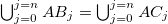 $\bigcup_{j=0}^{j=n} AB_{j} = \bigcup_{j=0}^{j=n} AC_{j}$
, where j ranges over the strata
$\bigcup_{j=0}^{j=n} AB_{j} = \bigcup_{j=0}^{j=n} AC_{j}$
, where j ranges over the strata
 $0, 0\mbox{-}ii, 0\mbox{-}iii, 1\mbox{-}i, \ldots, n\mbox{-}iii,n$
.
$0, 0\mbox{-}ii, 0\mbox{-}iii, 1\mbox{-}i, \ldots, n\mbox{-}iii,n$
.
Step 5: Step 4 showed that
 $A_{ncc}$
is an answer set of
$A_{ncc}$
is an answer set of
 $PA^{-}$
. Consider now program PA, that is, by reinstating the constraints into
$PA^{-}$
. Consider now program PA, that is, by reinstating the constraints into
 $PA^{-}$
. If none of the constraints is violated by
$PA^{-}$
. If none of the constraints is violated by
 $A_{ncc}$
then
$A_{ncc}$
then
 $A_{ncc}$
will be an answer set of PA. Suppose for contradiction that
$A_{ncc}$
will be an answer set of PA. Suppose for contradiction that
 $A_{ncc}$
is not an answer set of PA. This means that one or more of the constraints in PA must have been violated (i.e. the respective constraint body is satisfied) by
$A_{ncc}$
is not an answer set of PA. This means that one or more of the constraints in PA must have been violated (i.e. the respective constraint body is satisfied) by
 $A_{ncc}$
. There are two categories of constraints in PA, the pre-conditions in
$A_{ncc}$
. There are two categories of constraints in PA, the pre-conditions in
 $C_{pre}$
and the reactive rule constraint :- ant(ID,X,Ts),not consTrue(ID,X,Ts),time(Ts). There are two cases.
$C_{pre}$
and the reactive rule constraint :- ant(ID,X,Ts),not consTrue(ID,X,Ts),time(Ts). There are two cases.
Case 1:
 $A_{ncc}$
does not satisfy one of the constraints in
$A_{ncc}$
does not satisfy one of the constraints in
 $C_{pre}$
. By Step 2,
$C_{pre}$
. By Step 2,
 $A_{ncc}$
has the same fluents as
$A_{ncc}$
has the same fluents as
 $M_{P}$
up to time n. Also,
$M_{P}$
up to time n. Also,
 $A_{ncc}$
and
$A_{ncc}$
and
 $M_{P}$
have the same set of external events and by construction the same set of actions (the set H). Thus if
$M_{P}$
have the same set of external events and by construction the same set of actions (the set H). Thus if
 $A_{ncc}$
does not satisfy a pre-condition constraint, nor will
$A_{ncc}$
does not satisfy a pre-condition constraint, nor will
 $M_{P}$
, contradicting that
$M_{P}$
, contradicting that
 $M_{P}$
is a reactive model of P. Moreover, for a constraint that inhibits co-occurrence of events, all the events in the constraint have the same timestamp and if they all occur in
$M_{P}$
is a reactive model of P. Moreover, for a constraint that inhibits co-occurrence of events, all the events in the constraint have the same timestamp and if they all occur in
 $A_{ncc}$
, then they all occur in
$A_{ncc}$
, then they all occur in
 $M_{P}$
. For a constraint that imposes a pre-condition on an event, because the fluents in
$M_{P}$
. For a constraint that imposes a pre-condition on an event, because the fluents in
 $C_{pre}$
have timestamps earlier than an event in the same
$C_{pre}$
have timestamps earlier than an event in the same
 $C_{pre}$
rule, the fact that
$C_{pre}$
rule, the fact that
 $A_{ncc}$
has states only up to n does not matter.
$A_{ncc}$
has states only up to n does not matter.
Case 2:
 $A_{ncc}$
does not satisfy the reactive rule constraint. That is, for some id, x and t, ant(id,x,t) is true and consTrue(id,x,t) is false in
$A_{ncc}$
does not satisfy the reactive rule constraint. That is, for some id, x and t, ant(id,x,t) is true and consTrue(id,x,t) is false in
 $A_{ncc}$
. This means, by the definition of consTrue that there can be no Ts1
$A_{ncc}$
. This means, by the definition of consTrue that there can be no Ts1
 $\geq$
t in the range [
$\geq$
t in the range [
 $0, \ldots, n$
] such that cons(id,x,t,Ts1) is true. That is, there is a reactive rule in P with its antecedent true but for no time
$0, \ldots, n$
] such that cons(id,x,t,Ts1) is true. That is, there is a reactive rule in P with its antecedent true but for no time
 $\leq n$
can its consequent be made true. But that means there is a reactive rule in P that is not true in
$\leq n$
can its consequent be made true. But that means there is a reactive rule in P that is not true in
 $M_{P}$
, which is not the case.
$M_{P}$
, which is not the case.
5 Reactive ASP functionality beyond KELPS
In this section we describe how some features of ASP inherited by Reactive ASP can be exploited to enhance its flexibility and functionality beyond those of KELPS. The features we exploit are the model generation paradigm, weak constraints and the explicit representation of choice. More specifically, model generation allows reasoning to take into account any ramifications of actions (for prospective behaviour), in which Reactive ASP can look ahead to reason about possible evolutions of its current state, thus informing current decisions. Explicit choice and weak constraints allow to specify the type of model (pre-emptive, proactive or reactive) preferred and to rule out unwanted models and rank those models that are not ruled out. All of these new behaviours are possible because reactive ASP generates complete answer sets, and thus complete courses of actions and resulting fluents, up to a maximum time range n. In particular, we explain how to achieve pre-emptive, proactive and prospective reasoning, and introduce a hybrid system that combines the two frameworks of KELPS and ASP into one enhanced integrated framework that uses the best features of both.
Reasoning with Priorities
In KELPS all constraints are hard constraints and are used only to express pre-conditions of actions and to restrict co-occurrences of events. But in ASP constraints can be hard or soft (weak constraints) and can be used to express many other features, including preferences.
One useful application of preferences would be where the consequent is disjunctive and we would like to express preferences amongst the disjuncts. This can be achieved systematically when mapping to ASP as follows: Suppose the disjuncts in KELPS are written in order of preference from high to low. In the mapping to ASP, first give cons atoms an additional argument representing the position of a disjunct in the consequent of a rule; second, add the following generic weak constraint, which allows to prefer answer sets that achieve the lowest possible indexed disjunct.
 \begin{equation*}{\small\begin{array}{l}\texttt{{$:\sim$}cons(ID,I,Args,T,Ts).[1@I,ID,I,Args,T,Ts]}\end{array}}\end{equation*}
where the second argument of cons represents the position of the disjunct in the consequent of the reactive rule. For instance, the head of the second (apologise) disjunct in equation (2) might be written as the atom cons(1,2,(Cust,Item,T),T,Ts), where T represents the timestamp of the associated request. In this case the weak constraint ensures a preference for allocating items that are requested (I=1), if possible, rather than apologising (I=2).
We briefly mention some other typical examples, based around the bookstore narrative from Section 2, that demonstrate how constraints might be used to enhance decisions in Reactive ASP. As another example of using a weak constraint, we might want to prioritise allocation of items to a particular customer (say Tom) over any others in a situation where two customers requested the same item at the same time. This could be achieved by the constraint
 \begin{equation*}{\small\begin{array}{l}\texttt{$:\sim$happens(request(tom,Item),T),happens(request(C,Item),T),C!=tom,}\\\, \, \, \, \, \texttt{happens(allocate(tom,Item,_),T2),happens(allocate(C,Item,_),T1), }\\\, \, \, \, \, \texttt{time(T),time(T2),time(T1),T1<T2.[1@1,T,T1,T2,Item,C]}\end{array}}\end{equation*}
which penalises allocating the Item to customer C before allocating to Tom. Another example could be to prefer not to process more than one book at any time. This could be expressed by Footnote 25
 \begin{equation*}{\small\begin{array}{l}\texttt{$:\sim$happens(process(C1,Item1),T),happens(process(C2,Item2),T),}\\\, \, \, \, \, \texttt{time(T),Item1<Item2.[1@2,T,Item1,Item2,C1,C2]}\end{array}}\end{equation*}
One could even express a preference not to allocate items to the same customer within (say) three time steps. Other kinds of preferences could include: allocate as early as possible, or if an item requested by a customer is not in stock but is on order to be re-stocked then schedule the response to the customer’s order as late as possible (to avoid apologising unnecessarily). One could also consider more specific preferences, such as the one above, preferring to allocate books one at a time, but within that preferring to allocate children’s books as early as possible. This can be achieved by adding a second weak constraint at level 1. For instance
 \begin{equation*}{\small\begin{array}{l}\texttt{$:\sim$happens(request(C,Item),T1),child_book(Item)},\\\, \, \, \, \, \, \, \, \, \, \texttt{happens(allocate(C,Item,_),T2)},\\\, \, \, \, \, \, \, \, \, \, \texttt{time(T1),time(T2).[(T2-T1)@1,Item,T1,T2,C]}.\end{array}}\end{equation*}
will aim to minimise the time difference between a request and allocation of a children’s book.
In the next subsection we will show how to achieve pre-emptive, proactive and prospective behaviours in Reactive ASP.
5.1 Relaxing reactivity to provide a variety of other models
Recall that in KELPS the fact that all actions are supported is an emergent feature but in Reactive ASP this has to be formalised explicitly in the program. Below we explain how, by relaxing that actions be supported, a wider range of models can be generated by Reactive ASP leading to either pre-emption of a reactive rule, or proactive behaviour to satisfy a reactive rule. For instance, in case of an alarm in some building, the following KELPS reactive rule will produce a reactive model including the evacuate action only if no guard is present at the time of the alarm.
 \begin{equation}\begin{array}{l}alarm(T1) \wedge \neg present\_guard(T1) \\\, \, \, \, \, \rightarrow evacuate( T2) \wedge T1+1 < T2 \wedge T2< T1+4\end{array}\end{equation}
However, another possible model could be to pre-empt the alarm and send a guard to the building even before any alarm, so evacuation would not be needed. On the other hand, a proactive model might, as a precaution, evacuate a building even before any alarm! A more practical example of proactive behaviour could be to buy a ticket in advance of entering a bus to save time. Thus given the reactive rule
 $enter\_bus(T) \rightarrow have\_ticket(T_1) \wedge T \leq T_1\wedge T_1\leq T+1$
the ticket could be bought before entering the bus, ensuring that the fluent
$enter\_bus(T) \rightarrow have\_ticket(T_1) \wedge T \leq T_1\wedge T_1\leq T+1$
the ticket could be bought before entering the bus, ensuring that the fluent
 $have\_ticket$
holds when necessary. Neither of these behaviours is possible in KELPS as they are not supported by earlier conditions in a reactive rule, but by relaxing the supported condition for actions both behaviours can be achieved in our Reactive ASP formalism.
$have\_ticket$
holds when necessary. Neither of these behaviours is possible in KELPS as they are not supported by earlier conditions in a reactive rule, but by relaxing the supported condition for actions both behaviours can be achieved in our Reactive ASP formalism.
Firstly, any action that can be either pre-emptive or proactive is defined by a clause of the form action(act(
 $\bar{X}$
)):-body(
$\bar{X}$
)):-body(
 $\bar{X}$
) where act names the action, and body(
$\bar{X}$
) where act names the action, and body(
 $\bar{X}$
) represents a conjunction of auxiliary atoms used to ground
$\bar{X}$
) represents a conjunction of auxiliary atoms used to ground
 $\bar{X}$
, the set of arguments (if any) pertaining to that action.
$\bar{X}$
, the set of arguments (if any) pertaining to that action.
Secondly, the choice rule is simplified to enable actions of this kind to take place at any time T, whether supported or not: 0{happens(Act,Ts)}1:-action(Act),time(Ts),Ts>1. Actions that cannot be proactive or pre-emptive (i.e. are not defined by an action clause) are enabled, as before, by use of the supported predicate. As an example, in Figure 4 we illustrate how we can make actions send_guard and evacuate potentially proactive and pre-emptive. The figure also includes the ASP version of reactive rule (17). Footnote 26 This ASP program exhibits (or results in) several possible distinguishable behaviours via the models it generates. In some models a guard is sent at or before time 3 (pre-emptive behaviour); in some a guard is not sent and evacuation takes place at time 5 or 6 (reactive behaviour); and in others evacuation takes place at times from time 1 onwards (proactive behaviour).

Fig. 4. Security guard proactive and pre-emptive behaviour.
In the pre-emptive models the sending of the guard causes the antecedent condition not holds(present_guard,Ts) to be false by causing holds(present_guard,Ts) and avoiding evacuation. To prefer such behaviour a weak constraint can be used, such as the following, which minimises the number of evacuate actions, the best being zero: :∼ happens(evacuate,T),time(T).[1@2,T]. By making the priority level 2, this constraint will be minimised before any at a lower priority. Line 10 ensures that multiple occurrences of sending a guard are avoided, as a guard is sent only if one is not already present. Alternatively, the weak constraint :∼ happens(send_guard,T),time(T).[1@1,T] could be added to minimise the occurrences of the sending of guards (in addition to minimising the number of evacuates). This constraint can also be used on its own to minimise occurrences of sending a guard if proactive behaviour is preferred.
5.2 Prospective reasoning
KELPS agents are capable of non-deterministic self-evolution. At any given time, they may have several different possible future trajectories depending on what actions they take, when those actions are taken and what external situations arise. This provides an opportunity to explore what Pereira and others (Pereira and Lopes Reference Pereira and Lopes2009; Anh and Pereira Reference Anh and Pereira2011) call Prospection or Evolution Prospection. The challenge stated in prospective was “how to allow such evolving agents to be able to look ahead, prospectively, into such hypothetical futures, in order to determine the best courses of evolution from their own present, and thence to prefer amongst them”.
The advantage of Reactive ASP compared to the original KELPS is that it naturally incorporates Prospective reasoning and no further machinery is required. In particular, Recative ASP determines every possible course of actions and the corresponding set of ramifications (within a given time frame) and thus allows n-distant Prospective KELPS. It can also easily accommodate constraints and expected future events within that time frame. Thus each answer set would represent the agent’s possible future evolution within a fixed time frame of n cycles, with expected external scenarios. Furthermore, we can express “a priori” preferences for certain outcomes using strong and weak constraints, allowing to filter action plans and to highlight others in order of optimality. We will illustrate some of these features by an example.
Consider the following scenario related to decisions about what to drink and when to go to bed. There are three reactive rules: (i) if the agent drinks wine they must retire (to bed) within one cycle, due to drowsiness; (ii) if the sun sets the agent must also retire, but within three cycles; and (iii) if the agent is thirsty, they must have a drink (coffee, wine or water) before three cycles. Furthermore, there are some action pre-conditions: the agent cannot perform any action while asleep, nor, if the agent feels energetic, can they go to bed. Finally, there are some post-conditions: drinking coffee makes the agent energetic and going to bed induces sleep. Ideally, the agent wants to go to bed as late as possible. The scenario is expressed in the KELPS framework as shown in Figure 5. Footnote 27 Note that the above preference cannot be represented in KELPS.

Fig. 5. Example for prospection.
The corresponding mapping to Reactive ASP is standard and is in Figure A1 (in the Appendix). Imagine now that
 $S_0 = \{\}$
and
$S_0 = \{\}$
and
 $ext^*=\{thirsty(1)\}$
. So the agent must drink something and could choose coffee, wine, or water. Suppose we also know that sunset will occur at time 2. Then we can extend
$ext^*=\{thirsty(1)\}$
. So the agent must drink something and could choose coffee, wine, or water. Suppose we also know that sunset will occur at time 2. Then we can extend
 $ext^*=\{thirsty(1), sunset(2)\}$
and look ahead beyond the first 2 cycles, say up to time 5. Given the preference of going to bed as late as possible, the latest bedtime is time 5, after the sunset that occurs at time 2. As soon as the agent goes to bed it falls asleep and so can no longer drink. Thus the drinking can happen at the latest by time 5; in fact the latest is time 3 as it must be before time 4 according to the third reactive rule. Depending on which drink is chosen, there are various consequences. If coffee is chosen as the drink at time 2 or 3, then due to becoming energetic the agent will not be able to go to bed in time (and there will be no model). If wine is chosen at time 2 or 3, then the agent will have to go to bed at time 3 or 4, respectively, because of the first reactive rule. If water is chosen at time 2 or 3 then the agent need not go to bed until time 5. Of course, it is also possible to have multiple drinks, with similar consequences as above.
$ext^*=\{thirsty(1), sunset(2)\}$
and look ahead beyond the first 2 cycles, say up to time 5. Given the preference of going to bed as late as possible, the latest bedtime is time 5, after the sunset that occurs at time 2. As soon as the agent goes to bed it falls asleep and so can no longer drink. Thus the drinking can happen at the latest by time 5; in fact the latest is time 3 as it must be before time 4 according to the third reactive rule. Depending on which drink is chosen, there are various consequences. If coffee is chosen as the drink at time 2 or 3, then due to becoming energetic the agent will not be able to go to bed in time (and there will be no model). If wine is chosen at time 2 or 3, then the agent will have to go to bed at time 3 or 4, respectively, because of the first reactive rule. If water is chosen at time 2 or 3 then the agent need not go to bed until time 5. Of course, it is also possible to have multiple drinks, with similar consequences as above.
Reactive ASP provides all this information in the answer sets it produces, and the agent can then choose the best drinking option in the light of this. It is also possible to express preferences a priori, for example to minimise the number of drinks, or the aforementioned preference of going to bed as late as possible. These are achieved by weak constraints as in Lines 17 and 18 in Figure A1, repeated here.
 \begin{equation*}{\small\begin{array}{ll}17\mbox{.} & \texttt{$:\sim$happens(drink(L),T),isDrink(L),time(T).[1@1,T,L]}\\18\mbox{.} & \texttt{$:\sim$happens(gotoBed,T),time(T).[-T@2,T]}\\\end{array}}\end{equation*}
6 An integrated KELPS and reactive ASP framework
The discussions in the paper up to this point have highlighted the strengths of each of the two paradigms of Reactive ASP and KELPS. The major strength of Reactive ASP is that it easily allows a variety of reasoning behaviours and functionalities, such as prospective reasoning and reasoning with preferences via weak constraints. On the other hand major strengths of the KELPS OS are that it updates the state destructively and incrementally simplifies the reactive rules. Thus it does not reason with frame axioms, nor does it need to access past information about states or events. These respective strengths suggest a potential new architecture for reactive, prospective agents that combines KELPS and Reactive ASP. Such an architecture is summarised in Figure 6. The distribution of the work between the two paradigms in this architecture is informed by their relative strengths. We describe the architecture, henceforth abbreviated to HKA, and illustrate its behaviour through two examples.

Fig. 6. HKA: a combined architecture for reactive and prospective control.
In HKA the KELPS OS retains from Section 2 the parts of updating the state and triggering and simplifying the reactive rules in the light of changes to states and events, whereas the part of generation of plans to solve the goals is passed on to (prospective) Reactive ASP.
That is, in the KELPS module, at time T, the state is updated according to the events executed during the interval
 $[T-1,T)$
. Then the reactive rules are processed given the updated state at time T. The KELPS module then passes to Reactive ASP the updated state and all the processed reactive rules. Furthermore, if there happen to be anticipated external events in the future, these are also input to the Reactive ASP module. This module will have a time frame starting at T and ending at
$[T-1,T)$
. Then the reactive rules are processed given the updated state at time T. The KELPS module then passes to Reactive ASP the updated state and all the processed reactive rules. Furthermore, if there happen to be anticipated external events in the future, these are also input to the Reactive ASP module. This module will have a time frame starting at T and ending at
 $T+k$
(time(T.T+k)), for some chosen k, meaning that the search can consider up to k-distant models beyond the current time T. The value of k can vary in different iterations of the cycle if required.
$T+k$
(time(T.T+k)), for some chosen k, meaning that the search can consider up to k-distant models beyond the current time T. The value of k can vary in different iterations of the cycle if required.
The current state is modelled by holds(Args,T) and the future anticipated events at some time t>0 as happens(Args,t):-time(t). Since KELPS has processed all previous occurred events, there is no need for ASP to start its time range from earlier than T. We can illustrate this with a simple example. Let
 \begin{equation*}a(T) \wedge b(T+3) \rightarrow c(T1) \wedge T+3<T1 \wedge T1<T+6\end{equation*}
be a reactive rule in KELPS, where a, b and c are events, and suppose that a occurs at time 2. KELPS will partially process this rule to give a rule
 $b(5) \rightarrow c(T1) \wedge 5<T1 \wedge T1<8$
. It is this rule that is mapped into Reactive ASP for the time interval starting at time 2.
$b(5) \rightarrow c(T1) \wedge 5<T1 \wedge T1<8$
. It is this rule that is mapped into Reactive ASP for the time interval starting at time 2.
The rest of the Reactive ASP program, such as the causal theory and event theory remain as described in Section 3. Weak constraints formalising priorities and preferences can also be changed if desired with different iterations of the cycle.
The output from running the Reactive ASP part of HKA will be a set of optimal answer sets, according to the weak constraints, and looking forward in time from T to
 $T+k$
. From these answer sets and taking account of the external events in the next time interval [T,T+1), the best set of actions in this time interval to execute can be chosen. These are executed and combined with the external events and fed into the KELPS module for the next iteration at time
$T+k$
. From these answer sets and taking account of the external events in the next time interval [T,T+1), the best set of actions in this time interval to execute can be chosen. These are executed and combined with the external events and fed into the KELPS module for the next iteration at time
 $T+1$
.
$T+1$
.
Note that in HKA the ASP program has no need to reason about the past. In particular it will never need to instantiate the frame axiom in the event theory with time prior to the current cycle time, that is, prior to T in its time frame of time(T.T+k). It also does not need to reason with past events and states in respect to the reactive rules. We consider some simple examples of how this interaction works. For the first example, shown in Figure 7, we just describe the results.

Fig. 7. First Example for HKA interaction (
 $a1 - a8$
are events and p and q are fluents).
$a1 - a8$
are events and p and q are fluents).
Informally, from Figure 7 it can be seen that to satisfy rule R1 either a3 or a4 can occur at any time in the range [
 $2,\ldots,4$
], and to satisfy rule R2 either a6 may occur at any time in the range [
$2,\ldots,4$
], and to satisfy rule R2 either a6 may occur at any time in the range [
 $2,\ldots,9$
], or a7 can occur, but at or after time 6, after q is initiated by event a8. Suppose now that it is also the case that a7 is preferred to a6 in order to satisfy rule R2. It can be seen that in this situation rule R1 can only be satisfied by a4, because a3 terminates the pre-condition p of a7 before a7 can be usefully executed (because q would not be true). But after a4, a7 can occur at times 6, 7, 8 or 9. When translated into ASP at time 1 and run prospectively up to time 10, ASP will return as optimal answer sets the above results. The optimal answer sets are returned to KELPS, and KELPS makes a choice about the next action. It is worth noting that not only can KELPS by itself not deal with preferences, it cannot deal with foreknowledge of events such as a8 in the example when reasoning at earlier times.
$2,\ldots,9$
], or a7 can occur, but at or after time 6, after q is initiated by event a8. Suppose now that it is also the case that a7 is preferred to a6 in order to satisfy rule R2. It can be seen that in this situation rule R1 can only be satisfied by a4, because a3 terminates the pre-condition p of a7 before a7 can be usefully executed (because q would not be true). But after a4, a7 can occur at times 6, 7, 8 or 9. When translated into ASP at time 1 and run prospectively up to time 10, ASP will return as optimal answer sets the above results. The optimal answer sets are returned to KELPS, and KELPS makes a choice about the next action. It is worth noting that not only can KELPS by itself not deal with preferences, it cannot deal with foreknowledge of events such as a8 in the example when reasoning at earlier times.
Suppose an additional rule
 $R3: a7(T) \rightarrow a9(T1)\wedge T1=T+1$
is added to the example of Figure 7, and that it is also desired for a9 to be executed as late as possible. Then in a time frame extending from 1 to 10, a4 can occur as before and a7 should be executed at time 9, the latest time it can be to satisfy rule R2, to allow a9 to occur at time 10 and rule R3 to be satisfied.
$R3: a7(T) \rightarrow a9(T1)\wedge T1=T+1$
is added to the example of Figure 7, and that it is also desired for a9 to be executed as late as possible. Then in a time frame extending from 1 to 10, a4 can occur as before and a7 should be executed at time 9, the latest time it can be to satisfy rule R2, to allow a9 to occur at time 10 and rule R3 to be satisfied.
In the next example, shown in Figure 8, we illustrate the evolution of the ASP translation through several cycles. By way of illustration we assume that KELPS requests ASP to consider a time frame of 3 steps beyond the current time (i.e. k=3).

Fig. 8. Second Example for HKA interaction (here a and
 $a1-a3$
are events).
$a1-a3$
are events).
The prospective answer set from ASP in the time frame
 $\{1,\dots,4\}$
will suggest to execute a1 at time 2 or at time 3, allowing for a2 to be executed at time 3 or at time 4, respectively. Suppose that indeed a1(2) is executed, and furthermore foreknowledge of the external event a3(3) becomes available. Then it will become impossible to execute a2(3) because it would violate C
$\{1,\dots,4\}$
will suggest to execute a1 at time 2 or at time 3, allowing for a2 to be executed at time 3 or at time 4, respectively. Suppose that indeed a1(2) is executed, and furthermore foreknowledge of the external event a3(3) becomes available. Then it will become impossible to execute a2(3) because it would violate C
 $_{pre}$
. The only course of action to satisfy the reactive rule is for a1 to be executed again.
Footnote 28
Assuming that the time frame has now increased to
$_{pre}$
. The only course of action to satisfy the reactive rule is for a1 to be executed again.
Footnote 28
Assuming that the time frame has now increased to
 $\{2,\dots,5\}$
, then ASP will recommend re-executing a1 at time 3 (or time 4) to allow for a2 to be executed at time 4 (or time 5) in order to satisfy the reactive rule.
$\{2,\dots,5\}$
, then ASP will recommend re-executing a1 at time 3 (or time 4) to allow for a2 to be executed at time 4 (or time 5) in order to satisfy the reactive rule.
The operation of HKA relies on the following key observation: at each step of KELPS processing the reactive rules, the causal theory and the current state form a KELPS framework. In effect, the current state
 $S_{T}$
becomes the initial state for the next cycle (in Figure 6) and the conversion to k-distant KELPS and to Reactive ASP can be carried out as described in Section 3. In the sequel we will use the notation
$S_{T}$
becomes the initial state for the next cycle (in Figure 6) and the conversion to k-distant KELPS and to Reactive ASP can be carried out as described in Section 3. In the sequel we will use the notation
 $KELPS(T;T+k)$
to refer to the k-distant KELPS starting at time T. In Figure 9 we show the ASP rules resulting from mapping
$KELPS(T;T+k)$
to refer to the k-distant KELPS starting at time T. In Figure 9 we show the ASP rules resulting from mapping
 $KELPS(T;T+3)$
for Figure 8 at times
$KELPS(T;T+3)$
for Figure 8 at times
 $T = 0, 1, 2, 3$
. In this figure the numbering notation x.y indicates that x is the timestamp of the start of the time frame and y is an identifier for a reactive ASP rule. Thus rules with
$T = 0, 1, 2, 3$
. In this figure the numbering notation x.y indicates that x is the timestamp of the start of the time frame and y is an identifier for a reactive ASP rule. Thus rules with
 $x=0$
are the mapping of
$x=0$
are the mapping of
 $KELPS(0;3)$
into Reactive ASP. Rules with
$KELPS(0;3)$
into Reactive ASP. Rules with
 $x>0$
are the mapping of
$x>0$
are the mapping of
 $KELPS(x;x+3)$
. For example, at time 2 rule 2.3 is the result of processing the consequent of R due to the event a1(2), the antecedent of R having already become true because of the earlier event a(1). Original rules from previous timestamps are carried forward, unless otherwise indicated.
$KELPS(x;x+3)$
. For example, at time 2 rule 2.3 is the result of processing the consequent of R due to the event a1(2), the antecedent of R having already become true because of the earlier event a(1). Original rules from previous timestamps are carried forward, unless otherwise indicated.

Fig. 9. In the numbering notation x.y, x is the timestamp of the start of the time frame and y is an identifier for a reactive ASP rule. Thus rules with
 $x=0$
are the mapping of
$x=0$
are the mapping of
 $KELPS(0;3)$
into Reactive ASP. Rules with
$KELPS(0;3)$
into Reactive ASP. Rules with
 $x>0$
are the mapping of
$x>0$
are the mapping of
 $KELPS(x;x+3)$
.
$KELPS(x;x+3)$
.
By way of further illustration we highlight some of the results of these mappings. The rules 0.1 to 0.9 (called set 0) are a mapping of the framework
 $KELPS(0;3)$
from Figure 8. These rules, except 0.1 and 0.7, are maintained in subsequent frameworks. For example the constraints 0.8 and 0.6 are present in set 2, that maps
$KELPS(0;3)$
from Figure 8. These rules, except 0.1 and 0.7, are maintained in subsequent frameworks. For example the constraints 0.8 and 0.6 are present in set 2, that maps
 $KELPS(2;5)$
. The mapping of framework
$KELPS(2;5)$
. The mapping of framework
 $KELPS(1;4)$
(set 1) includes in addition the rules 1.1, 1.3-1.5, 1.7, and 1.8. The rules for time (e.g. rules 1.1) replace the old ones (e.g. 0.1) because of the shifting of the time window, that is rule time(0.k) is replaced by rule time(1.1+k). The new choice rule 1.7 replaces the old one (0.7) for the same reason, increasing the bound on Ts to the new start time of the framework. Similarly for transitions between times 1 and 2, etc. Rule 1.3 is the mapping of the processing by KELPS of rule R after the event a(1), which makes the antecedent of the rule true at time 1, leaving the instantiated consequent
$KELPS(1;4)$
(set 1) includes in addition the rules 1.1, 1.3-1.5, 1.7, and 1.8. The rules for time (e.g. rules 1.1) replace the old ones (e.g. 0.1) because of the shifting of the time window, that is rule time(0.k) is replaced by rule time(1.1+k). The new choice rule 1.7 replaces the old one (0.7) for the same reason, increasing the bound on Ts to the new start time of the framework. Similarly for transitions between times 1 and 2, etc. Rule 1.3 is the mapping of the processing by KELPS of rule R after the event a(1), which makes the antecedent of the rule true at time 1, leaving the instantiated consequent
 $a1(T1) \wedge 1<T1 \wedge a2(T2) \wedge T2=T1+1$
. The occurrence of event a(1) also results in the new supported rules 1.4 and 1.5. Since the antecedent of the reactive rule has been made true at time 1 the reactive rule constraint for that instance of the rule becomes the constraint 1.8 :-not consTrue(1,(1),1) indicating that rule R has not yet been satisfied. Similar explanations for the rules in set 2 and set 3 can be given. The rules in set 3 are the mapping of
$a1(T1) \wedge 1<T1 \wedge a2(T2) \wedge T2=T1+1$
. The occurrence of event a(1) also results in the new supported rules 1.4 and 1.5. Since the antecedent of the reactive rule has been made true at time 1 the reactive rule constraint for that instance of the rule becomes the constraint 1.8 :-not consTrue(1,(1),1) indicating that rule R has not yet been satisfied. Similar explanations for the rules in set 2 and set 3 can be given. The rules in set 3 are the mapping of
 $KELPS(3;6)$
, after action a1(3) and event a3(3). Notice also, that although some rule may have been satisfied, while actions in its consequent remain supported, ASP will still be able to generate those actions through the choice rule. This is why action a1(3) can occur as it is still supported (see rule 1.4).
$KELPS(3;6)$
, after action a1(3) and event a3(3). Notice also, that although some rule may have been satisfied, while actions in its consequent remain supported, ASP will still be able to generate those actions through the choice rule. This is why action a1(3) can occur as it is still supported (see rule 1.4).
We end this section by discussing the relationship between HKA and KELPS. First we define some terminology to use in our discussion.
Definition 6.1 Let
 $T\geq 0$
be a time and
$T\geq 0$
be a time and
 $KELPS(T;T+k) = <R_{T},\mathcal{C}$
,
$KELPS(T;T+k) = <R_{T},\mathcal{C}$
,
 $\mathcal{A}ux ,k>$
be a k-distant KELPS framework starting at time T with state
$\mathcal{A}ux ,k>$
be a k-distant KELPS framework starting at time T with state
 $S_{T}$
. Let
$S_{T}$
. Let
 $ev^{*}_{T+1}$
be events that take place during the time interval
$ev^{*}_{T+1}$
be events that take place during the time interval
 $[T,T+1)$
. Let these events transform the KELPS state
$[T,T+1)$
. Let these events transform the KELPS state
 $S_{T}$
to
$S_{T}$
to
 $S_{T+1}$
and process the reactive rules
$S_{T+1}$
and process the reactive rules
 $R_{T}$
to
$R_{T}$
to
 $R_{T+1}$
. We denote by
$R_{T+1}$
. We denote by
 $KELPS(T+1;T+1+k) = <R_{T+1}$
,
$KELPS(T+1;T+1+k) = <R_{T+1}$
,
 $\mathcal{C}$
,
$\mathcal{C}$
,
 $\mathcal{A}ux ,k+1>$
, the k-distant KELPS framework starting at time
$\mathcal{A}ux ,k+1>$
, the k-distant KELPS framework starting at time
 $T+1$
with state
$T+1$
with state
 $S_{T+1}$
. We denote the mapping of
$S_{T+1}$
. We denote the mapping of
 $KELPS(T;T+k)$
into ASP by
$KELPS(T;T+k)$
into ASP by
 $ASP(T;T+k)$
and the mapping ot
$ASP(T;T+k)$
and the mapping ot
 $KELPS(T+1;T+1+k)$
into ASP by
$KELPS(T+1;T+1+k)$
into ASP by
 $ASP(T+1;T+1+k)$
.
$ASP(T+1;T+1+k)$
.
We focus the discussion of the relationship between HKA and KELPS on the commutative diagram shown in Figure 10. In that figure the HKA approach we have described so far involves the mapping of
 $KELPS(T;T+k)$
to
$KELPS(T;T+k)$
to
 $ASP(T;T+k)$
(arrow m1), processing of the rules in
$ASP(T;T+k)$
(arrow m1), processing of the rules in
 $KELPS(T;T+k)$
in the light of events that take place during the time interval
$KELPS(T;T+k)$
in the light of events that take place during the time interval
 $[T;T+1)$
and the resulting updated state to obtain
$[T;T+1)$
and the resulting updated state to obtain
 $KELPS(T+1;T+1+k)$
(arrow m2), and a mapping of this to
$KELPS(T+1;T+1+k)$
(arrow m2), and a mapping of this to
 $ASP(T+1;T+1+k)$
(arrow m3). In addition, of course, as indicated in Figure 6,
$ASP(T+1;T+1+k)$
(arrow m3). In addition, of course, as indicated in Figure 6,
 $ASP(T;T+k)$
feeds back to
$ASP(T;T+k)$
feeds back to
 $KELPS(T;T+k)$
information about computed answer sets, as does
$KELPS(T;T+k)$
information about computed answer sets, as does
 $ASP(T+1;T+1+k)$
to
$ASP(T+1;T+1+k)$
to
 $KELPS(T+1;T+1+k)$
.
$KELPS(T+1;T+1+k)$
.

Fig. 10. Relationship between KELPS(
 $T;T+k$
) and ASP(
$T;T+k$
) and ASP(
 $T;T+k$
).
$T;T+k$
).
It is worth noting that the soundness and completeness results of Section 4 naturally extend to the mappings in m1 and m3, based on the aforementioned key observation that at each step of KELPS processing the reactive rules, the causal theory and the current state form a KELPS framework. But as can be seen in Figure 10 there is an alternative, more economical, approach to realising HKA, namely the following. There is an initial mapping of
 $KELPS(0;k)$
to
$KELPS(0;k)$
to
 $ASP(0;k)$
, but after that, at each time
$ASP(0;k)$
, but after that, at each time
 $T>0$
after KELPS provides the executed events and the updates state to ASP, it is possible to mirror in ASP itself the (KELPS-style) processing of the reactive rules to obtain the new
$T>0$
after KELPS provides the executed events and the updates state to ASP, it is possible to mirror in ASP itself the (KELPS-style) processing of the reactive rules to obtain the new
 $ASP(T;T+k)$
. This is indicated by arrow m4 in Figure 10. This avoids the need for mappings of KELPS into ASP after
$ASP(T;T+k)$
. This is indicated by arrow m4 in Figure 10. This avoids the need for mappings of KELPS into ASP after
 $T>0$
. In the following we define the direct mapping between
$T>0$
. In the following we define the direct mapping between
 $ASP(T;T+k)$
and
$ASP(T;T+k)$
and
 $ASP(T+1;T+1+k)$
. This correspondence between KELPS and its mapping to ASP relies on the fact KELPS processing of the reactive rules is based on resolution. Moreover, since both ASP and KELPS are logic-based languages the resolution step is defined identically for the two, and thus each mirrors the other. We formalise this idea next in Definition 6.2.
$ASP(T+1;T+1+k)$
. This correspondence between KELPS and its mapping to ASP relies on the fact KELPS processing of the reactive rules is based on resolution. Moreover, since both ASP and KELPS are logic-based languages the resolution step is defined identically for the two, and thus each mirrors the other. We formalise this idea next in Definition 6.2.
Definition 6.2 Given
 $ASP(T;T+k)$
, a set of events in the form happens(e, T+1), in the time interval
$ASP(T;T+k)$
, a set of events in the form happens(e, T+1), in the time interval
 $[T,T+1)$
and a set of fluents, in the form holds(f,T+1),
$[T,T+1)$
and a set of fluents, in the form holds(f,T+1),
 $ASP( T+1;T+1+k)$
is constructed through 5 steps as follows:
$ASP( T+1;T+1+k)$
is constructed through 5 steps as follows:
Step 1: Increment time. Replace time facts time(T.T+k) with time(T+1.T+1+k) and replace the condition
 $T<Ts$
in the choice rule with
$T<Ts$
in the choice rule with
 $T+1<Ts$
.
$T+1<Ts$
.
Step 2: Reason with events and fluents at time T + 1. Apply inference to rules in
 $ASP(T;T+k)$
using facts of the form happens(e,T+1) and holds(f,T+1).
$ASP(T;T+k)$
using facts of the form happens(e,T+1) and holds(f,T+1).
Step 3: Simplify using Aux and time facts. Remove from rule bodies all ground and true time atoms (i.e. inference with the time facts added in Step 1). Remove all true negated happens and holds literals, and negated
 $\mathcal{A}ux$
literals.
$\mathcal{A}ux$
literals.
Step 4: Propagate new facts timestamped T + 1. Apply inference to rules using any newly generated facts timestamped
 $T+1$
(e.g. ant and cons) with rules.
$T+1$
(e.g. ant and cons) with rules.
Step 5: Remove processed facts and constraints. Except for any newly generated consTrue fact, remove facts timestamped
 $T+1$
which were reasoned with in Step 4. Remove rules which now have unsatisfiable body conditions. This latter step may apply to ground constraints of the form :-not consTrue(ID,Args,Ts) which were generated at a time Ts earlier than the current time
$T+1$
which were reasoned with in Step 4. Remove rules which now have unsatisfiable body conditions. This latter step may apply to ground constraints of the form :-not consTrue(ID,Args,Ts) which were generated at a time Ts earlier than the current time
 $T+1$
.
$T+1$
.
We use Figure 9 to exemplify some of the reasoning described in Definition 6.2. The rules 1.3 to 1.5 and 1.8 are instances of rules in set 0 that have been derived using facts at time 1. Rule 0.2 is resolved with the facts happens(a,1) and time(1) (Steps 2 and 3) to give ant(1,(1),1), which in turn is resolved with rule 0.3 to give 1.3, and with rule 0.8 to give 1.8 (Step 4). Similar derivations yield the other rules. If the constraint 0.6 were not present, action a2 could occur at time 3 making cons(1,(1),1,3) true. This would allow consTrue(1,(1),1) to be derived from 0.9 (Step 4) and the constraint 1.8 to be satisfied, whence it can be removed because it would have an unsatisfiable body condition (Step 5). In the case of the actual example in Figure 9, since 0.6 is present, this cannot occur and constraint 1.8 remains in set 3 as shown.
7 Discussion and related work
In this section we review the translation of KELPS to ASP and the variations considered, before discussing related work.
7.1 Brief review of reactive ASP
The basic concepts of KELPS were described in Section 2.1, in which, to progress towards achieving the goals specified by the reactive rules, and in the light of new observations, at each time point supported actions can be selected for execution provided their pre-conditions hold. KELPS models are not time limited, so for translating to ASP, which produces finite models, the notion of an n-distant KELPS framework was introduced (see Definition 3.1). The basic restriction is that time is limited to the interval
 $[0, \ldots, n]$
for some given value of n and no events can occur after n, nor can the notion of supportedness require that time extend beyond n.
$[0, \ldots, n]$
for some given value of n and no events can occur after n, nor can the notion of supportedness require that time extend beyond n.
The translation of n-distant KELPS into ASP was described in subsections 3.1 to 3.3 and proven sound and complete in Section 4. A feature of the translation is the ability to include pre-emptive and proactive, as well as reactive, behaviour. This is facilitated by the flexibility of how to specify explicitly in the program what actions can be selected, as well as by prioritising models with weak constraints, as we saw in Section 5. Another feature of the translation we illustrated in Section 5 is the ability to include prospective behaviour. This is essentially the basic mapping, but the focus is different. In this case foreknowledge of possible future events is made available to improve the decision making at the current time. This feature is not possible in KELPS, but simply emerges as a consequence of the ASP translation.
The two paradigms KELPS and Reactive ASP differ in their operational behaviour. In KELPS the framework reasons partially about the consequences of reactive rules and interleaves the reasoning with action execution. Thus, a KELPS framework may execute an action as part of a partial evaluation of a consequent and simply verify that the temporal constraints will allow a model to exist potentially. Of course, future (as yet unknown) events, or consequences of future actions, might still prevent the existence of such a potential model. On the other hand, Reactive ASP, being a model generation paradigm, generates complete answer sets and thus complete plans up to a maximum time n, and it is this that makes prospective reasoning possible. Even so, it is possible that an answer set of a reactive ASP program exists at some time t, but no answer set including it exists for longer time frames because of new observations made after time t. Another major difference between the two paradigms is that KELPS requires no frame reasoning, but Reactive ASP requires reasoning with the explicit frame axiom in the event theory (rule 14 in Figure 3).
These differences encouraged the design of a hybrid KELPS/ASP paradigm that benefits from the destructive update of actions and the consequences on fluents that is inherent in KELPS, yet also uses prospection as a way of providing information about the “best” actions to be selected for execution at each increasing time point. In an architecture described in Section 6 for this hybrid the initial KELPS program is translated into ASP, and then at each later time step ASP recommends the next set of actions to be executed through prospective reasoning taking into account any anticipated future events up to a required time point, and KELPS executes the actions and returns to ASP via the translation the updated state and partially evaluated reactive rules. The period of prospection can vary as required, for example at each time step. This hybrid system is able to simulate an extended KELPS framework incorporating prospective reasoning over some possibly varying set k of future times, the prospective time frame being
 $[currentTime \dots currentTime+k ]$
, where currentTime increases by 1 at each iteration. This system is quite close to the operational semanitics of KELPS in the sense of committing to actions as time progresses. In fact, the models computed by the ASP program at cycle t can be characterised as follows. They are the KELPS
$[currentTime \dots currentTime+k ]$
, where currentTime increases by 1 at each iteration. This system is quite close to the operational semanitics of KELPS in the sense of committing to actions as time progresses. In fact, the models computed by the ASP program at cycle t can be characterised as follows. They are the KELPS
 $t+k$
-distant models of the initial state of KELPS together with the executed events (observed events and user actions) up to time t and the anticipated external events at times
$t+k$
-distant models of the initial state of KELPS together with the executed events (observed events and user actions) up to time t and the anticipated external events at times
 $t+1$
up to
$t+1$
up to
 $t+k$
.
$t+k$
.
7.2 A possible alternative incremental ASP mapping
The OS of KELPS, as depicted in Figure 1, is inherently incremental in nature. As time progresses the database is updated destructively, new events are observed and actions are considered to make the consequents of reactive rules true, once their antecedents are satisfied. In effect, KELPS (resp. n-distant KELPS) attempts to construct model structures (resp. n-distant model structures) based on current knowledge, for each time step k,
 $k \geq 0$
(resp.
$k \geq 0$
(resp.
 $0 \leq k\leq n$
).
$0 \leq k\leq n$
).
We initially had a concern that in the basic translation of Section 3, here called the standard mapping, the frame axiom in the event theory of Reactive ASP might render the system unscalable, as regards the size of the grounding of the program, and the time taken to generate the grounding and find solutions.
Therefore, in addition to what we have described so far we implemented a slightly different mapping of n-distant KELPS to ASP utilising the incremental variant of clingo 4. The models returned by the implementation are found incrementally, from inital time 0 up to final time n. Assuming the same external events, the effect is the same as if the standard mapped program were run iteratively in a loop for times varying from 0 through n. That is, for each time t in the range
 $[0, \ldots, n ]$
there is an answer set if and only if KELPS has a t-distant model, and the answer sets correspond to the KELPS models in the sense of Section 4. Recall from Section 3 that the sets of models of n-distant frameworks for different values of n are generally not the same, even when the external events are unchanged. Therefore, in the incremental approach the models must be, and are, re-computed for each t in the range
$[0, \ldots, n ]$
there is an answer set if and only if KELPS has a t-distant model, and the answer sets correspond to the KELPS models in the sense of Section 4. Recall from Section 3 that the sets of models of n-distant frameworks for different values of n are generally not the same, even when the external events are unchanged. Therefore, in the incremental approach the models must be, and are, re-computed for each t in the range
 $[0, \ldots, n ]$
.
$[0, \ldots, n ]$
.
To compare the two approaches, we ran two simple experiments. The first experiment recorded the rate of time increase for a program resulting from the standard mapping, with external events, but with no reactive rule or reactive rule integrity constraint, and so the only reasoning involved the causal theory, including its frame axiom. The experiment was made for increasing numbers of fluents and/or steps. The second experiment compared the overall time for running individual calls to the standard mapped program for n varying from 0 up to a given maximum with that for running the incremental mapped program for the same given maximum. The results are shown in Tables B1 and B2 in the Appendix. It is clear from the results of the first experiment that the overhead of using the frame axiom is linear in the value of the maximum timestamp and linear in the number of fluents, which is as expected, but acceptable. The results of the second experiment show that there is no gain in using the incremental mapping.
Note also that the Hybrid HKA framework would not require long time frames in each run of the ASP part, and moreover it would reduce the need for reasoning with the frame axiom by limiting it only to the future events. Another motivation for considering the incremental approach was that it could allow for external events to be added by the user at each time step at the time they happen. However, the Hybrid HKA achieves this in a more flexible way, and moreover incorporates prospective reasoning as well. Therefore, although the use of incremental clingo seemed an obvious mode for the translation, we did not find any particular advantage, and did not pursue it further, but for completeness we have described it in the Appendix.
7.3 Other approaches to reactivity in logic programming
Reactivity, in the context of KELPS, has a specific meaning (see Section 2.1.4). In Kowalski and Sadri (Reference Kowalski and Sadri2015) (Section 7) and Kowalski and Sadri (Reference Kowalski and Sadri2016) (Section 6) KELPS has been compared extensively with related work, such as abductive logic programming, event calculus, MetateM, constraint handling rules, production systems, transaction logic, active databases, agent languages and reactive systems programming languages.
Reactivity has also been explored in Action Logics. The paper (Baral and Son Reference Baral and Son1998) describes reactive control theories, where each control rule has on the left-hand side (analogous to our antecedent) a conjunction of fluents all referring to the same time, and on the right-hand side (analogous to our consequent) a conjunction of actions all to be performed at the same time. The language is quite restrictive in comparison to KELPS, and its purpose is to show the correctness of such reactive control with respect to causal theories of action. Reactivity has been incorporated in two extensions of the Action Language
 $\mathcal{A}$
, which added triggers, initially to give a language
$\mathcal{A}$
, which added triggers, initially to give a language
 $\mathcal{A}_{o}^{T}$
(Tran and Baral Reference Tran and Baral2004), and then further extended to a language
$\mathcal{A}_{o}^{T}$
(Tran and Baral Reference Tran and Baral2004), and then further extended to a language
 $\mathcal{A}_{\infty}^{T}$
(Nam and Baral Reference Nam and Baral2007). The triggers in
$\mathcal{A}_{\infty}^{T}$
(Nam and Baral Reference Nam and Baral2007). The triggers in
 $\mathcal{A}_{o}^{T}$
have the restricted syntax of fluents holding in a single state triggering an action that must take place at the time it is triggered.
$\mathcal{A}_{o}^{T}$
have the restricted syntax of fluents holding in a single state triggering an action that must take place at the time it is triggered.
 $\mathcal{A}_{\infty}^{T}$
provides more flexibility than
$\mathcal{A}_{\infty}^{T}$
provides more flexibility than
 $\mathcal{A}_{o}^{T}$
by allowing the triggered action to take place at the same time it is triggered or later. Separately from, and independently of, the reactive rules,
$\mathcal{A}_{o}^{T}$
by allowing the triggered action to take place at the same time it is triggered or later. Separately from, and independently of, the reactive rules,
 $\mathcal{A}_{\infty}^{T}$
allows for event orderings. However, in KELPS this is incorporated in the consequents of reactive rules making the event orderings related to the context of the triggers and reactions. In addition KELPS allows histories of states and events in antecedents and consequents of reactive rules. One similar aspect between
$\mathcal{A}_{\infty}^{T}$
allows for event orderings. However, in KELPS this is incorporated in the consequents of reactive rules making the event orderings related to the context of the triggers and reactions. In addition KELPS allows histories of states and events in antecedents and consequents of reactive rules. One similar aspect between
 $\mathcal{A}_{\infty}^{T}$
and KELPS is that the definition of state transitions in
$\mathcal{A}_{\infty}^{T}$
and KELPS is that the definition of state transitions in
 $\mathcal{A}_{\infty}^{T}$
captures the intuition that if an action occurs then it must have been triggered. This intuition is similar to the notion of supportedness of actions in KELPS.
$\mathcal{A}_{\infty}^{T}$
captures the intuition that if an action occurs then it must have been triggered. This intuition is similar to the notion of supportedness of actions in KELPS.
In the work described in this paper we use ASP to generate KELPS reactive models, and to our knowledge there is no other work that incorporates such reactivity in ASP. But there is other work that uses ASP to incorporate different perspectives of reactivity. We briefly review these below. The oclingo system (Gebser et al. Reference Gebser, Grote, Kaminski and Schaub2011) was an early “reactive” answer set solver, whose technology has been incorporated into clingo 4. This solver generates answer sets incrementally, taking into account new information in real-time. It is reactive to the extent that the answer sets grow and change, as new information is acquired. Vaseqi and Delgrande (Reference Vaseqi and Delgrande2013) suggest using this technology as a “situational awareness” tool in maritime traffic domains. This allows new information to be acquired (and inferred) over time, and thus it allows managing the histories that form dynamically over several time steps.
In Ribeiro et al. (Reference Ribeiro, Inoue and Bourgne2013) the authors also propose using ASP for reactive reasoning. However, their notion of reactivity is about the efficiency of reasoning and generation of models. They achieve this efficiency by dividing the agent knowledge into modules. Only relevant modules are solved at any given step, avoiding the computational cost of generating irrelevant knowledge. In this sense the agent can then “react” more quickly to its given situation. The ASP modules form a tree-like hierarchy, starting at a “root” and spreading to “leaves”. The root and the internal nodes represent the agent’s knowledge about itself (meta-knowledge), and the leaves represent “elementary knowledge” (such as what actions should be taken). At every step, the reasoning process starts at the root, which determines the next module(s) to solve; this process continues until leaf nodes are reached. The meta-reasoning determines what the agent needs to know in the given context. It is not necessary to reason about all available knowledge at every step.
In Costantini (Reference Costantini2011) the author uses ASP in conjunction with Observe-Think-Act agents. For each possible external event, a “reactive ASP module” defines the different ways in which the agent might react to it. Each module contains a constraint, satisfied only when the relevant external event occurs. When the relevant event occurs, the resulting set of models indicates possible reaction strategies. In this work the ASP modules can be triggered only by single events. By contrast, in KELPS, and consequently in Reactive ASP, a reactive rule can be triggered by a conjunction of events and conditions. In fact, in KELPS and in Reactive ASP a reactive rule is in general triggered by a history of events and state conditions, and the reactions, in general, are plans extending over periods of time. In Reactive ASP, moreover, using weak constraints and prospection we can compare different models to determine which action plan has the most desirable future ramifications.
In Costantini et al. (Reference Costantini, De Gasperis and Nazzicone2015) the authors describe a combined architecture between DALI agents (Costantini and Tocchio Reference Costantini and Tocchio2004) and an answer set program that performs planning tasks and determines what actions the agent can take. However, these modules do not indicate which action will lead to the best outcome, nor do they provide the reactive or prospective reasoning of the KELPS-Reactive ASP hybrid.
In a more recent position paper (Dyoub et al. Reference Dyoub, Costantini and De Gasperis2018) the authors argue for a modular design also exploiting features of ASP in combination with agent architectures. No specific design is given, but in principle our hybrid architecture can be said to be motivated by similar considerations. In fact, the authors seem to be of the opinion that ASP is not a “fully appropriate modelling tool for the dynamic flexible functioning of agents as concerns reactivity, proactivity and communication”.
In Section 5 we discussed how our formalisation of reactivity in ASP lends itself to prospection. We saw that no further notation or functionality was required to cater for this. The use of clingo and the approach to modelling KELPS agents allows us to look into the future for a given time frame and also to take into account not only the present information and its ramifications, but also any known information about the future and its ramifications.
A logic programming system called ACORDA for prospective reasoning is proposed in Pereira and Lopes (Reference Pereira and Lopes2009) and applied to modelling multi-agent intention recognition in Anh and Pereira (Reference Anh and Pereira2011) and morality in Pereira and Saptawijaya (Reference Pereira and Saptawijaya2011). In the latter the authors formalise classic trolley problems, where action or inaction in diverting a trolley has implications in terms of lives saved. In their system abductive hypotheses are generated for solving goals. Then some reasoning is performed from the abducibles to obtain relevant consequences, which can then be compared according to specified preferences. This work does not use temporal information and does not specify how far into the future one wishes to prospect. Moreover, it does not incorporate knowledge about known future events or states. Another significant difference with our work is that, as well as exploring the consequences of abductions Footnote 29 , we explore their other ramifications in terms of triggering a chain of new reactions in the future, via the reactive rules and changes of state.
Specific applications of reactivity that KELPS/LPS can be and has been considered for are formalisation and monitoring of policies as well as active updates in databases. It would be interesting to consider how Reactive ASP might be exploited for such applications, for example as described in Eiter et al. (Reference Eiter, Fink, Sabbatini and Tompits2004). Moreover, KELPS/LPS provides an aspect of stream processing, as described in Section 2.1.2. The KELPS OS monitors the stream of states and incoming and self-generated events and actions, to check whether an instance of a reactive rule antecedent has become true and to determine if any actions have become necessary. It processes the stream on the fly, that is, as it receives it. It would be interesting to see how Reactive ASP might be exploited to do stream reasoning, for example as in Beck et al. (Reference Beck, Dao-Tran and Eiter2018).
A different formalism using equilibrium temporal logic to model reactive rules is described in Cabalar et al. (Reference Cabalar, Kaminski, Schaub and Schuhmann2018). A recent system called tclingo, presented in Cabalar et al. (Reference Cabalar, Kaminski, Schaub and Schuhmann2018) and based on temporal Equilibrium Logic (Aguado et al. Reference Aguado, Cabalar, Dieguez, Perez and Vidal2013), has some similarities to KELPS. Specifically, the temporal rules are restricted as in KELPS such that antecedent atoms contain no future operators and consequent atoms contain no past operators. However, the logic is propositional and thus appears to be less expressive than KELPS.
8 Conclusion and future work
This paper has described how the form of reactivity captured within the KELPS system (Kowalski and Sadri Reference Kowalski and Sadri2016) can be implemented in ASP. Moreover, it has shown that the resulting ASP representation is, in some respects, more flexible than KELPS in that it allows for proactive and pre-emptive behaviour and prospective reasoning. In addition, a Hybrid KELPS/ASP that combines the advantages of both frameworks was described.
Although the mapping to ASP required to include explicitly a frame axiom, this has not caused particular runtime problems. We acknowledge that in case of simulations with a very large number of constants and/or a very long time span, the running time or grounding of the answer set program could become a problem. However, our intention is not to deal with long timespans. For example in the proposed Hybrid the timespan would relate to the prospective future. Moreover, one of our motivations to model KELPS in ASP was to facilitate the implementation of various analysis tools by exploiting the representation, for instance to detect inconsistencies in a Reactive ASP program. This too does not need a long timestamp. Such analysis tools would be useful because the presence of temporal constraints and action pre-conditions in KELPS makes it difficult to judge a priori if the reactive rules are satisfiable, and there is a need for an automated system that makes this decision. For example, the reactive rule constraint could be modified by adding a head atom as in
 \begin{equation*}{\small\begin{array}{ll}\texttt{badRule(ID,Args,Ts):-ant(ID,Args,Ts), not consTrue(ID,Args,Ts),time(Ts).}\end{array}}\end{equation*}
to detect cases where an antecedent of some reactive rule is true but the corresponding consequent cannot be satisfied. Minimising occurrences of badRule atoms would show if this kind of inconsistency can happen and under what circumstances.
We also will extend the implementation of Reactive ASP to include the full LPS, including conditional clauses in the causal theory and complex events. Recent work, such as Suchan and Bhatt (2019), has addressed the problem of detecting complex events from video. Such approaches could contribute to a longer term goal, namely a more complex reasoning system encompassing detection of external events as well as reasoning about the ramifications of the events. Reactive ASP will also allow us to have more expressive clauses in the causal theory, whereby for example pre-conditions of actions can refer to histories of past events and states. Of interest also, is the potential to learn reactive rules due to the systematic structure of the resulting ASP program. In our future work we will use the state-of-the-art inductive learning system ILASP (Law et al. Reference Law, Russo and Broda2016) to learn reactive rules given example models of the expected behaviour.
Acknowledgements
We thank the anonymous reviewers for their helpful and insightful comments. We also thank Bob Kowalski for useful discussions on an early draft of the paper.


B. Alternative KELPS simulation
This section presents an alternative incremental style mapping from n-distant KELPS to ASP (called multi-shot). As in Section 3 we will consider n-distant KELPS frameworks and throughout we use as an example the KELPS framework shown in Figure B1. We assume that for the n-distance version appropriate temporal constraints are added to the two reactive rules, according to Definition 3.1.

Fig. B1. KELPS Framework for exemplifying incremental simulation.
B.1 An incremental (multi-shot) mapping for computing
$\textbf{n}$
-distant models

In this appendix we make use of clingo 4 to incrementally increase the time frame, and to incrementally generate groundings. We use a predicate maxRange/1 to represent the horizon for the increasing timespan.
The mapping from n-distant KELPS to Reactive ASP given in Section 3 employed a global time frame from time 0 to time n. We refer to that mapping as
 $f_{global}$
. In this section we describe a second, incremental mapping, which we refer to as
$f_{global}$
. In this section we describe a second, incremental mapping, which we refer to as
 $f_{inc}$
. The difference between the two mappings can most clearly be seen at a qualitative level by considering the translation of a very simple reactive rule of the form
$f_{inc}$
. The difference between the two mappings can most clearly be seen at a qualitative level by considering the translation of a very simple reactive rule of the form
 \begin{equation}{\textit{R}:}\ \ event(T) \rightarrow action(T_1) \wedge T+1 < T_1\end{equation}
by ant and cons rules as well as a reactive rule constraint. First of all, recall that using
 $f_{global}$
the translation would include the rules
$f_{global}$
the translation would include the rules
 \begin{equation}{\small \begin{array}{l}\texttt{ant(id,(Ts),Ts):-happens(event,Ts),time(Ts).}\\\texttt{cons(id,(T),T,Ts):-ant(id,(T),T),happens(action,Ts),T+1<Ts,time(Ts).}\\\texttt{:-ant(Id,X,Ts),not consTrue(Id,X,Ts),time(Ts).}\\\texttt{consTrue(Id,X,Ts):-cons(Id,X,Ts,Ts1),time(Ts1).}\\ \texttt{supported(action,Ts):-ant(id,(T),T),T+1<Ts,time(Ts).} \end{array}}\end{equation}
Note that (in this example) in the definition of cons the head of the rule has a timestamp that is at least two timestamps after the timestamp of the matching ant in the body, but all appropriate groundings of the rules are considered at once. In particular, this means that the time variables are constrained to be in the range [
 $0,\ldots,n$
], as given by the facts time(0.n).
$0,\ldots,n$
], as given by the facts time(0.n).
On the other hand, the basic mapping
 $f_{inc}$
(for a fixed value of n given by maxRange(n)) enlists the parameterised subprogram feature of clingo 4. The resulting (multi-shot) program consists of two subprograms (or modules), which we call base and cycle(t) declared by the #external program command and whose grounding is under control of a procedure “Control” (shown in Figure B3 and described in subsection B.2). The base subprogram is a standard ASP program representing the initial state, the auxiliary facts
$f_{inc}$
(for a fixed value of n given by maxRange(n)) enlists the parameterised subprogram feature of clingo 4. The resulting (multi-shot) program consists of two subprograms (or modules), which we call base and cycle(t) declared by the #external program command and whose grounding is under control of a procedure “Control” (shown in Figure B3 and described in subsection B.2). The base subprogram is a standard ASP program representing the initial state, the auxiliary facts
 $\mathcal{A}ux$
and
$\mathcal{A}ux$
and
 $C_{post}$
. The cycle(t) subprogram consists of rules for ant, cons and supported, the reactive rule integrity constraint, and the choice rule, as well as the event theory ET and
$C_{post}$
. The cycle(t) subprogram consists of rules for ant, cons and supported, the reactive rule integrity constraint, and the choice rule, as well as the event theory ET and
 $C_{pre}$
. The timestamp argument for all these is t. The procedure Control will generate an instantiation of cycle(t) for each value of t in the program’s overall time frame (i.e. t =1,2,3,… n), where n is fixed by a maxRange fact in the module base. Each new instantiation is added incrementally to the pre-existing program. So, if the program models n cycles, it will eventually include the modules base and cycle(1), cycle(2),…, cycle(n). The (ground) program is resolved after each cumulative expansion. Considering the reactive rule in (B1), but now using the mapping
$C_{pre}$
. The timestamp argument for all these is t. The procedure Control will generate an instantiation of cycle(t) for each value of t in the program’s overall time frame (i.e. t =1,2,3,… n), where n is fixed by a maxRange fact in the module base. Each new instantiation is added incrementally to the pre-existing program. So, if the program models n cycles, it will eventually include the modules base and cycle(1), cycle(2),…, cycle(n). The (ground) program is resolved after each cumulative expansion. Considering the reactive rule in (B1), but now using the mapping
 $f_{inc}$
, the mapped rules, which will be in cycle(t), will have the form in (B3)
$f_{inc}$
, the mapped rules, which will be in cycle(t), will have the form in (B3)
 \begin{equation}{\small \begin{array}{l}\texttt{ant(id,(t),t):-happens(event,t).} \\\texttt{cons(id,(T),T,t):-ant(id,(T),T),happens(action,t),T+1<t.}\\\texttt{:-query(t), ant(Id,X,T),not consTrue(Id,X,T,t).}\\\texttt{consTrue(Id,X,T,t):-cons(Id,X,T,T1).}\\\texttt{supported(action,t):-ant(id,(T),T),T+1<t.} \end{array}}\end{equation}
As before, in the definitions of ant and cons the final parameter (t) is the timestamp at which the head atom of rule becomes true. The atom query(t) is an external atom declared in ASP by the command #external query(t) and whose truth value can be manipulated by the procedure Control (see Figure B3). Consider, for example, the grounding of the constraint when t=3 and query(3)=True, which will require that for every previously true ground instance of ant(ID,X,T) (i.e. T
 $\leq 3$
), there must be a true atom cons(ID,X,T,T1), where T1 takes a value in the range [
$\leq 3$
), there must be a true atom cons(ID,X,T,T1), where T1 takes a value in the range [
 $0,\ldots,3$
]. There was a previous grounding of the constraint, when t=2 and query(2)= True, which required for every previously true ground instance of ant(ID,X,T) (i.e. T
$0,\ldots,3$
]. There was a previous grounding of the constraint, when t=2 and query(2)= True, which required for every previously true ground instance of ant(ID,X,T) (i.e. T
 $\leq 2$
), that there must be a true atom cons(ID,X,T,T1), where T1 takes a value in the range [
$\leq 2$
), that there must be a true atom cons(ID,X,T,T1), where T1 takes a value in the range [
 $0,\ldots,2$
]. It can be seen that for each value of t the constraint requires that for all previous true atoms of ant(ID,X,T) (T
$0,\ldots,2$
]. It can be seen that for each value of t the constraint requires that for all previous true atoms of ant(ID,X,T) (T
 $\leq $
t) there must be a true atom cons(ID,X,T,T1), where T1 takes a value in the range [0,…,t]. Eventually, when t=n the same set of instances of the constraint will have been considered as for the global mapping.
$\leq $
t) there must be a true atom cons(ID,X,T,T1), where T1 takes a value in the range [0,…,t]. Eventually, when t=n the same set of instances of the constraint will have been considered as for the global mapping.
Using this incremental grounding,
 $f_{inc}$
, the mapped rules for the example in Figure B1 are shown in Figure B2. To map the observed external events
$f_{inc}$
, the mapped rules for the example in Figure B1 are shown in Figure B2. To map the observed external events
 $ext^*=\{a(1), b(5), c(9)\}$
, the facts happens(a,1), happens(b,5) and happens(c,9) can be made available to the modules cycle(1), cycle(5) and cycle(9), as shown in Lines 6a-6c in Figure B2. The maximum timespan is fixed by Lines 1a and 1b (for illustration we used 10). This can be overrridden by another value on the program call to clingo. The extratime atom used in the body of the definition for supported in Line 14 ensures that there is adequate future time for the remaining parts of the (consequent of the reactive) rule to be made true. Here, the existential variable T2 is a time in the future of t, and is constrained to be within the maximum range of 10.
$ext^*=\{a(1), b(5), c(9)\}$
, the facts happens(a,1), happens(b,5) and happens(c,9) can be made available to the modules cycle(1), cycle(5) and cycle(9), as shown in Lines 6a-6c in Figure B2. The maximum timespan is fixed by Lines 1a and 1b (for illustration we used 10). This can be overrridden by another value on the program call to clingo. The extratime atom used in the body of the definition for supported in Line 14 ensures that there is adequate future time for the remaining parts of the (consequent of the reactive) rule to be made true. Here, the existential variable T2 is a time in the future of t, and is constrained to be within the maximum range of 10.

Fig. B2. Translation by
 $f_{inc}$
of example in Figure B1.
$f_{inc}$
of example in Figure B1.
B.2 The procedural control
To implement the incremental variant of Reactive ASP we have used clingo 4 (Gebser et al. Reference Gebser, Kaminski, Kaufmann, Lindauer, Ostrowski, Romero, Schaub, Thiele and Wanko2019), with a simple Lua script, similar to that given in (Gebser et al. Reference Gebser, Kaminski, Kaufmann and Schaub2019b) (see Figure B3). The input max to the procedure is extracted from the constant m on Line 1a of the ASP program.
In the first cycle (
 $t=0$
) the base program is solved, capturing the initial state,
$t=0$
) the base program is solved, capturing the initial state,
 $\mathcal{A}ux$
and information about post-conditions of events. In the next cycle (
$\mathcal{A}ux$
and information about post-conditions of events. In the next cycle (
 $t=1$
) the procedure does the following steps. It sets query(1) to True, effectively “activating” the reactive rule constraint for the time frame 0 to 1 (see Lines 8a and 8b in Figure B2) and attempts to find the program’s answer sets. To look for answer sets in subsequent time frames (
$t=1$
) the procedure does the following steps. It sets query(1) to True, effectively “activating” the reactive rule constraint for the time frame 0 to 1 (see Lines 8a and 8b in Figure B2) and attempts to find the program’s answer sets. To look for answer sets in subsequent time frames (
 $t=1,\ldots, max$
) it is necessary to “switch off” the constraint for the time frame 0 to 1 and to re-try it with an expanded time frame. To this end, the procedural control sets query(1) to False, sets query(2) to True and adds the instantiated cycle(2), and tries to find an answer set without redoing the grounding of the previous iteration. This loop continues until t=max.
Footnote 30
$t=1,\ldots, max$
) it is necessary to “switch off” the constraint for the time frame 0 to 1 and to re-try it with an expanded time frame. To this end, the procedural control sets query(1) to False, sets query(2) to True and adds the instantiated cycle(2), and tries to find an answer set without redoing the grounding of the previous iteration. This loop continues until t=max.
Footnote 30
By way of illustration, some relevant parts of the output of the program in Figure B2 with the control in Figure B3 are described next for the value of the constant m set to 7. There is one answer set for
 $t=0$
, namely {holds(p,0)}.
Footnote 31
There is no answer set for
$t=0$
, namely {holds(p,0)}.
Footnote 31
There is no answer set for
 $t=1$
or
$t=1$
or
 $t=2$
because the agent cannot yet satisfy the reactive rule triggered by happens(a,1). However, for
$t=2$
because the agent cannot yet satisfy the reactive rule triggered by happens(a,1). However, for
 $t=3$
the agent can perform the actions a1 and a2 and satisfy the rule consequent of the reactive rule with identifier 1. The resulting answer set includes the atoms {happens(a,1),happens(a1,2),happens(a2,3),holds(p,0), holds(p,1)}. For
$t=3$
the agent can perform the actions a1 and a2 and satisfy the rule consequent of the reactive rule with identifier 1. The resulting answer set includes the atoms {happens(a,1),happens(a1,2),happens(a2,3),holds(p,0), holds(p,1)}. For
 $t=4$
there are two answer sets, depending on whether action a1 occurs at time 2, or time 3. For
$t=4$
there are two answer sets, depending on whether action a1 occurs at time 2, or time 3. For
 $t=5$
there is no answer set since there is no time to perform b1 to satisfy the reactive rule with identifier 2. Moreover, in order for b1 to occur the fluent p must be true in the previous time instant, hence action a1 must not have occurred at least until time 6. This prevents any answer set for
$t=5$
there is no answer set since there is no time to perform b1 to satisfy the reactive rule with identifier 2. Moreover, in order for b1 to occur the fluent p must be true in the previous time instant, hence action a1 must not have occurred at least until time 6. This prevents any answer set for
 $t=6$
as there is no time to satisfy reactive rule with identifier 1. There is an answer set for
$t=6$
as there is no time to satisfy reactive rule with identifier 1. There is an answer set for
 $t=7$
, namely {happens(a,1),happens(a1,6),happens(a2,7), happens(b,5),happens(b1,6),holds(p,0),holds(p,1),holds(p,2),holds(p,3),holds(p,4), holds(p,5)}. Note that for each value of t, where there is an answer set it corresponds to a t-distant KELPS reactive model - and vice versa.
$t=7$
, namely {happens(a,1),happens(a1,6),happens(a2,7), happens(b,5),happens(b1,6),holds(p,0),holds(p,1),holds(p,2),holds(p,3),holds(p,4), holds(p,5)}. Note that for each value of t, where there is an answer set it corresponds to a t-distant KELPS reactive model - and vice versa.

Fig. B3. Pseudocode procedural control.
B.3 Experiments
We show here results of two experiments. The first experiment checks the impact of the explicit frame axiom in the standard mapping of Section 3, while the second experiment compares the standard mapping with the incremental version of Section B.1.
The first experiment (actually two sub-experiments 1a and 1b), involved a standard mapping program with the potential to vary the number of fluents. Specifically, the fluents belonged to
 $\{p(X),q(X),r(X),s(X),t(X),j(X) : 1\leq X\leq 200\}$
. There were 6 external events,
$\{p(X),q(X),r(X),s(X),t(X),j(X) : 1\leq X\leq 200\}$
. There were 6 external events,
 $\{c, d, e, f, g, h\}$
, each having 9 occurrences at varying times between 1 and 100. The action post-conditions were initiates(c,p(X)), initiates(d,q(X)), initiates(e,r(X)), initiates(f,s(X)), initiates(g,t(X)), initiates(h,j(X)), and terminates(c,q(X)), terminates(d,r(X)), terminates(e,p(X)), terminates(f,j(X)), terminates(g,s(X)), terminates(h,t(X)), for
$\{c, d, e, f, g, h\}$
, each having 9 occurrences at varying times between 1 and 100. The action post-conditions were initiates(c,p(X)), initiates(d,q(X)), initiates(e,r(X)), initiates(f,s(X)), initiates(g,t(X)), initiates(h,j(X)), and terminates(c,q(X)), terminates(d,r(X)), terminates(e,p(X)), terminates(f,j(X)), terminates(g,s(X)), terminates(h,t(X)), for
 $1\leq X\leq 200$
.
Footnote 32
There were no reactive rules.
$1\leq X\leq 200$
.
Footnote 32
There were no reactive rules.
Experiment 1a fixed the maximum timestamp at 200 and varied the number of fluents by changing the number of indices (X) in steps of 20 up to 200. Experiment 1b fixed the number of fluents at 1200 (
 $X=200$
) and ran for maximum timestamps (n) varying from 100 up to 1000 in steps of 100. Results of both experiments are shown in Table B1. It is clear that, as expected, the total runtime varies linearly with the number of fluents and with the maximum timestamp.
$X=200$
) and ran for maximum timestamps (n) varying from 100 up to 1000 in steps of 100. Results of both experiments are shown in Table B1. It is clear that, as expected, the total runtime varies linearly with the number of fluents and with the maximum timestamp.
Table B1. Results of Experiment 1a (left) and Experiment 1b (right)

The second experiment compared run times of the standard mapping from Section 3 with those of the incremental version. The program was an extended version of that shown in Figure B2, with external events
 $a(1) \ldots a(3)$
and
$a(1) \ldots a(3)$
and
 $b(1) \ldots b(3)$
occurring at various times. In this experiment, as in Figure B2, there is again one nullary fluent p. Just as in Figure B2, where the event a triggers events a1 and a2, in this extended version event a(I) triggers a1(I) and a2(I). The reactive rules are the same except that the events a, a1, a2, b and b1 are modified by adding an index ranging from 1 to 3 and adjustments made accordingly. The experiment ran the standard Reactive ASP code for every value of maximum timestamp between 1 and 50 and accumulated the execution times in groups of 10 or 20. It compared the results for the incremental translation for maxRange (m) values in
$b(1) \ldots b(3)$
occurring at various times. In this experiment, as in Figure B2, there is again one nullary fluent p. Just as in Figure B2, where the event a triggers events a1 and a2, in this extended version event a(I) triggers a1(I) and a2(I). The reactive rules are the same except that the events a, a1, a2, b and b1 are modified by adding an index ranging from 1 to 3 and adjustments made accordingly. The experiment ran the standard Reactive ASP code for every value of maximum timestamp between 1 and 50 and accumulated the execution times in groups of 10 or 20. It compared the results for the incremental translation for maxRange (m) values in
 $\{10,20,40,50\}$
. The results are shown in Table B2.
$\{10,20,40,50\}$
. The results are shown in Table B2.
Table B2. Results of Experiment 2

The external events occurred at the following times:
 $\{(a(1),1), (b(1), 5), (a(2), 11), (b(2), 15), (a(3), 32), (b(3), 35), (c,9),(c,19),(c,29),(c,39),(c,49)\}$
. All indexed a1 events terminate fluent p and all indexed b1 events require the fluent p to hold at the previous time. The purpose of event c was to (re)initiate the fluent p after it had been terminated, ready for each subsequent pair of events a and b. Additionally, some constraints were imposed to limit the number of occurrences of actions a1(I), a2(I), b1(I),
$\{(a(1),1), (b(1), 5), (a(2), 11), (b(2), 15), (a(3), 32), (b(3), 35), (c,9),(c,19),(c,29),(c,39),(c,49)\}$
. All indexed a1 events terminate fluent p and all indexed b1 events require the fluent p to hold at the previous time. The purpose of event c was to (re)initiate the fluent p after it had been terminated, ready for each subsequent pair of events a and b. Additionally, some constraints were imposed to limit the number of occurrences of actions a1(I), a2(I), b1(I),
 $I \in \{1,2,3\}$
, to a maximum of one each and to ensure that the reactions a1(I), a2(I) and b1(I) to an occurrence of events a(I) and b(I) occur before the occurrence of a and b with the next index (i.e.
$I \in \{1,2,3\}$
, to a maximum of one each and to ensure that the reactions a1(I), a2(I) and b1(I) to an occurrence of events a(I) and b(I) occur before the occurrence of a and b with the next index (i.e.
 $a(I+1)$
and
$a(I+1)$
and
 $b(I+1)$
) – see equation (B4), shown for the incremental version.
$b(I+1)$
) – see equation (B4), shown for the incremental version.
 \begin{equation}{\small \begin{array}{l}\texttt{:-happens(a1(X),T),happens(a1(X),t),T<t,index(X).}\\\texttt{:-happens(a2(X),T),happens(a2(X),t),T<t,index(X).}\\\texttt{:-happens(b1(X),T),happens(b1(X),t),T<t,index(X).}\\ \texttt{:-happens(b1(X),t),happens(a2(X),T1),t>T1,index(X).} \end{array}}\end{equation}
The results show that the cumulative time for n standard runs is lower than the incremental time. As mentioned earlier, it is to be expected that the times be comparable as the incremental program has to re-evaluate the set of models for each value of t up to n. The results show there is a small additional overhead.


 Open access