


Excessive weight, especially obesity, is a major public health concern in the western world. Around two-thirds of the adult population in the USA and at least half of the population of many European countries are currently overweight or obese (Berghöfer et al., Reference Berghöfer, Pischon, Reinhold, Apovian, Sharma and Willich2008; Flegal et al., Reference Flegal, Carroll, Ogden and Curtin2010; Wang et al., Reference Wang, Beydoun, Liang, Caballero and Kumanyika2008). In the Netherlands, the prevalence of overweight is 48.3% (Volksgezondheid, Nationaal Kompas, 2012), and 12.7% of the Dutch population is classified as obese. It is known that obesity — defined as a BMI of 30 or more — is a major risk factor for many chronic diseases, such as hypertension, stroke, coronary heart disease, diabetes, arthritis and overall mortality (Flegal et al., Reference Flegal, Kit, Orpana and Graubard2013; Prospective Studies Collaboration et al., Reference Whitlock, Lewington, Sherliker, Clarke, Emberson and Peto2009). Furthermore, increased BMI has also been shown to be associated with reduced physical health-related quality of Life (HRQoL) (Ul-Haq et al., Reference Ul-Haq, Mackay, Fenwick and Pell2012, Reference Ul-Haq, Mackay, Fenwick and Pell2013). However, evidence on the relationship between BMI and mental HRQoL is inconclusive. Some studies have found that BMI is associated with poor mental health (Baumeister & Härter, Reference Baumeister and Härter2007; Ohayon, Reference Ohayon2007; Petry et al., Reference Petry, Barry, Pietrzak and Wagner2008), whereas others did not find such a relationship (Crisp & McGuiness, Reference Crisp and McGuiness1976; Goldney et al., Reference Goldney, Dunn, Air, Dal Grande and Taylor2009; Palinkas et al., Reference Palinkas, Wingard and Barrett-Connor1996; Petry et al., Reference Petry, Barry, Pietrzak and Wagner2008). Ul-Haq et al. (Reference Ul-Haq, Mackay, Fenwick and Pell2014) also found that the association between BMI and mental health among the Scottish adult population (N = 37,272) was moderated by age and sex. In contrast to the above-mentioned studies, Ul-Haq et al. (Reference Ul-Haq, Mackay, Fenwick and Pell2014) used the full spectrum of BMI and adjusted for potential confounders and found that only young obese women (<45 years of age with BMI >29.9 kg/m2) had significantly reduced mental health. Furthermore, being underweight was also associated with diminished mental health among women of all ages, but not men.
Background on Lifelines
Lifelines is a large, population-based cohort study and biobank investigating the biological, behavioral and environmental determinants of healthy aging among 167,729 inhabitants from the northern part of the Netherlands. The cohort profile of the Lifelines study has been extensively described in Scholtens et al. (Reference Scholtens, Smidt, Swertz, Bakker, Dotinga, Vonk and Stolk2015). Summarizing, the participants’ baseline visit took place between December 2006 and December 2013. All general practitioners in the three northern provinces of the Netherlands were asked to invite their registered patients aged 25–49 years. All persons who consented to participate were asked to provide contact details to invite their family members (i.e., partner, parents and children), resulting in a three-generation study. In addition, participants could also register their participation via the Lifelines website. Lifelines adopted a multigenerational study design to disentangle the genetic, lifestyle and environmental contributions to the development of chronic diseases, study the between-generation similarities and identify the preclinical stages of ageing at an early age (Stolk et al., Reference Stolk, Rosmalen, Postma, de Boer, Navis, Slaets and Wolffenbuttel2008). Baseline data were collected from 167,729 participants, aged from 6 months to 93 years. Follow-up is planned for at least 30 years, with questionnaires administered every 1.5 years and a physical examination scheduled every 5 years. The physical examinations, including anthropometry, lung function, blood pressure, electrocardiogram (ECG) and cognition tests, are conducted at one of the Lifelines research sites. In addition, fasting blood and 24-h urine samples are collected from all participants. A comprehensive questionnaire on history of (chronic) diseases, HRQoL, lifestyle (physical activity, alcohol use, diet and smoking status), individual socioeconomic status (income and education level), psychosocial stress, work (profession, working hours), psychosocial characteristics and medication use is completed at home.
Lifelines is a facility that is open to all researchers. Information on application and data access procedure is summarized on www.lifelines.net. An overview of the available data is presented in the online Lifelines Data Catalogue.
Motivation and Goal
Although the explicit familial structure of the data is an advantage in studying the genetic and environmental components of various health-related outcomes, it is in fact a complicating factor in studying the effect of traditional epidemiological covariates. Given that participants are related (e.g., grandparent–grandchild, parent–child, and sibling–sibling relations), genetic, shared environmental and health behavioral factors may confound the effects of BMI on physical and mental HRQoL.
The standard way to control for familial effects is through the kinship model (Almasy & Blangero, Reference Almasy and Blangero1998), which is a variance components model whereby genetic relatedness is modeled through a kinship covariance matrix. Despite the genetic plausibility of the model, it is computationally prohibitive for thousands of individuals and hundreds of families. This means that it cannot be used for the Lifelines study.
Our first objective is to study the effect of BMI on mental and physical components of HRQoL scores with and without accounting for relatedness in a family. Another objective is to determine a computationally efficient model that incorporates genetic and shared environment to assess the contribution of epidemiological determinants on health outcomes. Given the large sample size and inclusion of extended families in the study, Lifelines allows the identification of the effect of relatedness with higher precision than other studies that are often (much) smaller and limited to particular types of family relationships (e.g., Lichtenstein et al., Reference Lichtenstein, Yip, Björk, Pawitan, Cannon, Sullivan and Hultman2009; Noh et al., Reference Noh, Yip, Lee and Pawitan2006; Pawitan et al., Reference Pawitan, Reilly, Nilsson, Cnattingius and Lichtenstein2004; Rabe-Hesketh et al., Reference Rabe-Hesketh, Skrondal and Gjessing2008; Yip et al., Reference Yip, Björk, Lichtenstein, Hultman and Pawitan2008). The current Lifelines study includes extended families with up to 19 members.
Not only are the variance components due to specific factors of interest, but also the relative contribution of these variances in the total variance of the outcome. Related to this is the concept of intraclass correlation coefficient (ICC). The ICC represents the heritability coefficient in a narrow sense when applied to additive genetic models. The concept of heritability originates from Fisher (Reference Fisher1918) and Wright (Reference Wright1920) and was formalized by Lush (Reference Lush1940). An extensive review on the concept and misconceptions of heritability is given by Visscher et al. (Reference Visscher, Hill and Wray2008). In the Methods section, we provide the definitions of shared environmental, unique environmental and hereditary ICCs in the context of our models. We also briefly introduce the beta-approach (Demetrashvili et al., Reference Demetrashvili, Wit and Van den Heuvel2016) to construct confidence intervals for the ICC. The beta-approach has been successfully applied to construct confidence intervals for ratios of sums of variance components in linear and nonlinear mixed-effects models (Demetrashvili & Van den Heuvel, Reference Demetrashvili and Van den Heuvel2015). This approach will use the first and second moments of the ICC estimate in combination with a beta distribution for accurate confidence intervals.
In the next section, we provide the background on the reconstruction of families and outcome measures. Then we describe various models and give a motivation of their use, including criteria for their selection. Following, we provide the analysis of familial confounding of BMI-related physical and mental HRQoL in the Lifelines study. We then compare our fractional relatedness model with more traditional kinship models through simulations. We conclude the article with an extensive discussion.
Methods
In this section, we explain how we reconstructed extended families from the available local kinship relationships. The outcomes of interest are mental and physical health, which were reconstructed from a RAND-36 questionnaire. Then we applied mixed-effects models beside a fixed-effect model to study the effect of BMI on mental and physical health.
Family Reconstruction
For a large number of participants in the Lifelines study, their parents, partner and children are also included in the study. Such information is relevant for disentangling the genetic, behavioral and shared environmental variances. In biometric genetics, the coefficient of relatedness or genetic correlation for two individuals is defined as the expected proportion of genes of two individuals that are identical by descent (Sham, Reference Sham1998, p. 208). A related concept in biometric genetics, which is used in this study, is that of a founder. Individuals without ancestors in the study are called founders, whereas others are called non-founders (Almgren et al., Reference Almgren, Bendahl, Bengtsson, Hössjer and Perfekt2003, p. 10). Founders in our study population are assumed unrelated.
Considering the information provided by Lifelines participants, we define a family as a group of related individuals sharing environmental and/or genetic factors. For example, health responses of mother and child may be similar due to both genetic similarity and shared behavior and environment, whereas the health responses of partners are related only due to the latter. Within the context of the Lifelines study, we define the concept of an extended family as a connected graph of individuals either via parent–child or partner–partner relationships. An example of a family is given in Figure 1. Note that the sibling relationships in this graph are inferred from common parent relationships. Sibling information itself is not recorded within Lifelines. We do not have extensive information for all reconstructed families in the Lifelines study, as some members might not participate in the study.
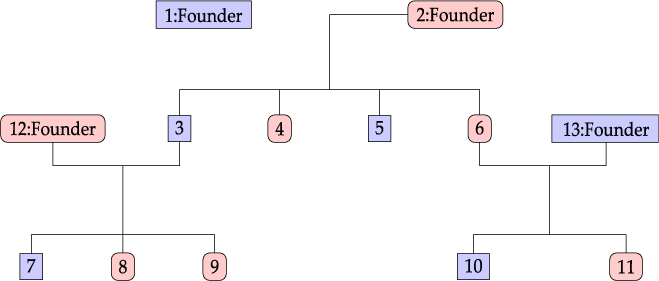
Fig. 1. Family example consisting of 13 members.
Information on children from previous marriages is, in principle, also available. However, not all familial information is complete in Lifelines, since people may not be willing, for example, to identify ex-partners. Some of the information, however, can be reconstructed from the partial information provided by the participants. For example, if a child declares both parents and the parents declare this child, but do not declare each other as partners, we make a link between such parents as a couple. For family reconstruction, we identify a set of related individuals through parent–child and/or partner–partner relationships and call this set a family. Once an individual is assigned to a particular family, no further reassignments take place. The model we propose in this study requires construction of the relatedness matrix. Relatedness between founders and non-founders is fractional, as explained in the next section. In Table 1, we outline the algorithm used for construction of fractional relatedness matrix.
Table 1. Algorithm for Construction of a Fractional Relatedness Matrix

Outcome Measures
A sample consisting of 91,759 participants from the baseline Lifelines cohort study data release was available for analysis. HRQoL was measured using the Dutch version of the RAND-36 questionnaire (Hays & Morales, Reference Hays and Morales2001; Van der Zee & Sanderman, Reference Van der Zee and Sanderman1993; Van der Zee et al., Reference Van der Zee, Sanderman, Heyink and de Haes1996). HRQoL refers to how health impacts on an individual’s ability to function and his or her perceived well-being in physical, mental and social domains of life. The RAND-36 consists of 36 items measuring eight health concepts, that is, physical functioning, role limitations caused by physical health problems, bodily pain, general health perceptions, role limitations caused by emotional problems, social functioning, emotional well-being, and energy/fatigue. The first four reflect the physical health and the last four reflect the mental health of an individual. The scales of these eight concepts are combined into two summary measures of HRQoL, the physical component score (PCS) and the mental component score (MCS), using the scoring algorithm of Ware et al. (Reference Ware, Kosinski and Keller1994). PCS and MCS are between 0% and 100% and higher scores correspond to better quality of life.
Statistical Models
We compare four models to examine whether the effect of BMI on HRQoL differs with and without accounting for family structure. These models are: M0: multiple regression model; M1: mixed-effects model with random intercept for the family, capturing the environmental familial effect; M2: mixed-effects model with random slopes for founders within a family, capturing the genetic familial effect. The fourth model, M3, is a combination of the last two models. Thus, M3 is a mixed-effects model with random intercept for family and random slopes for founders, capturing both environmental and genetic familial effects.
Assume that a total of n individuals and I families are included in the study. Suppose for the ith family ni members have been observed (i = 1, 2, …, I), such that  $n = \sum\limits_{i = 1}^I {{n_i}} $. The multiple regression model M0 of the HRQoL response yij for the jth member of the ith family can be written as:
 $${y_{ij}} = {\bf{x}}_{ij}^T\beta + {\varepsilon _{ij}},$$
where xij is a p × 1 vector for the jth individual in the ithfamily measured on p covariates, including BMI and possible confounders, β is a p × 1 vector of coefficients and residual errors ɛij across all observations are assumed to be identically and independently distributed (iid) having a normal distribution with mean zero and variance  $\sigma_{R}^{2},\,{\varepsilon_{ij}}\mathop\sim\limits^{iid} N(0,\sigma _R^2)$. The fixed effects xij can be quantitative or dummy variables to represent categorical variables, so the effective number of covariates may be less or equal to p.
Note, observations yij within the same family are most likely correlated, but the multiple regression model M0 does not account for this. Model M1 will account for this correlation by introducing a random intercept ui for every family:
 $${y_{ij}} = {\bf{x}}_{ij}^T\beta + {u_i} + {\varepsilon _{ij}},$$
where ui is normally distributed with mean zero and variance  $\sigma _R^2,\,{u_i}\mathop\sim\limits^{iid} N(0,\sigma _u^2)$; the definitions of xij, β and ɛij are the same as in (1).
Model M1 does not disentangle the genetic and shared environmental variation. Since one of the goals is to estimate the variance contribution in MCS and PCS due to various factors, model M2 will assume that the genetic correlation between family members is due to additive genetic effects of alleles (with no dominant and epistatic effects). By assuming all genetic information is in the founders, and consequently imposing the fractional relatedness effect between founders and other members of the family, model M2 introduces the random slopes υi for the set of founders mi in family i and can be formulated as:
 $${y_{ij}} = {\bf{x}}_{ij}^T\beta + {\bf{F}}_{ij}^T{\upsilon _i} + {\varepsilon _{ij}}$$
where definitions of xij, β and ɛij are the same as in (1) and Fij is the mi × 1 vector of founders for individual j in family I, where Fijk is a fractional relatedness of individual j to founder k in family i with  $\sum\limits_{k = 1}^{{m_i}} {{F_{ijk}}} = 1$; υi is the mi × 1 vector of random slopes for founders in family I, where υi = (υi 1, … υim), ${\upsilon _{ik}}\mathop\sim\limits^{iid} N(0,\sigma _f^2)$. We assume independence between random terms.
An important computational advantage of model M2 compared to the traditional kinship model is employment of a substantially smaller design matrix Fij. Namely, in M2, the design matrix across all families is of size m by n, where m is the maximum number of founders among all families and n is the total number of participants in all families. In the classical kinship model, the variance component matrix would be of size n by n. Dimensionality reduction is particularly crucial when one analyzes large number of participants, such as in Lifelines.
An example of a family consisting of 13 members in the Lifelines study is shown in Figure 1: oval shapes refer to females and squares to males. The associated fractional relatedness matrix F is demonstrated below. The M2 model assumes that the health outcome has a hereditary component. For example, the founders F1 and F2 both share half of their random hereditary effects with their child, member 3, and one-quarter with their grandchild, member 7.
 $$Fi = \left( {\matrix{ 1 \cr 2 \cr 3 \cr 4 \cr 5 \cr 6 \cr 7 \cr 8 \cr 9 \cr {10} \cr {11} \cr {12} \cr {13} \cr } \left| {\matrix{ {F1} & {F2} & {F12}&{F13} \cr 1& 0 & 0 & 0 \cr 0&1&0 & 0 \cr {1/2} & {1/2} & 0 & 0 \cr {1/2} & {1/2} & 0 & 0 \cr {1/2} & {1/2} & 0 & 0 \cr {1/2} & {1/2} & 0 & 0 \cr {1/4} & {1/4} & {1/2} & 0 \cr {1/4} & {1/4} & {1/2} & 0 \cr {1/4} & {1/4} & {1/2} & 0 \cr {1/4} & {1/4} & 0 & {1/2} \cr {1/4} & {1/4} & 0 & {1/2} \cr 0 & 0 & 1 & 0 \cr 0 & 0 & 0 & 1 \cr } } \right.} \right)$$
Model M3 is a combination of models M1 and M2, and can be written:
 $${y_{ij}} = {\bf{x}}_{ij}^T\beta + {u_i} + {\bf{F}}_{ij}^T{\upsilon _i} + {\varepsilon _{ij}},$$
where definitions and assumptions used in models M1 and M2 remain the same for this model. Variance components  $\sigma _u^2, \sigma _f^2 \, {\rm {and}} \,\sigma _R^2$ are due to shared environmental, genetic and unique factors, respectively.
Inference and Model Selection
The overall significance of each covariate is tested using a conditional F test. In this test, as in the usual F test of covariates for regression models, the conditional estimate of the residual error variance is used. More details on the F test are given in Pinheiro and Bates (Reference Pinheiro and Bates2009, §2.4.2). Confidence intervals for marginal coefficients βl are constructed based on conditional t tests. Each fixed-effect coefficient can be tested marginally in the presence of other fixed effects in the model (Pinheiro & Bates, Reference Pinheiro and Bates2009, pp. 92–96). The approximate 100% (1−α) confidence limits on the βl are computed as:
 $${\hat \beta _l} \pm t{}_{df{}_l}(1 - \alpha /2){\sqrt {\hat var(\hat \beta )} _{ll}},$$
where  ${\hat \beta _l}$ is an estimate of lth fixed effect, ${t_{d{f_l}}}(q)$ denotes the qth quantile of a t distribution with $d{f_l}$ degrees of freedom and $\hat var{(\hat \beta )_{ll}}$ is an estimate of the variance of ${\hat \beta _l}$. Clearly $\hat var(\hat \beta )$ is the variance–covariance matrix of the vector $\hat \beta $ of fixed-effects estimates. More on the determination of the degrees of freedom for our model is in the below ‘Estimation of fixed effects’ section.
To select the best model we used the Bayesian information criterion (BIC; Schwarz, Reference Schwarz1978). The BIC for these models is defined as:
 $${\rm{BIC}}(M) = - 2{l_M}(\theta |y) + df(M)\ln (n),$$
where  ${l_M}( \cdot )$ is the log-likelihood function for the estimated model M with θ a vector of all parameters, df(M) denotes the overall number of parameters in the model, that is, the regression and variance components parameters and n is the total number of observations used to fit the model. The model with the smallest BIC is preferred.
Intraclass Correlation Coefficient
The models we defined above allow us to define the following three types of ICC: (1) the behavioral and shared environmental ICC (c 2), as the proportion of total variance due to shared environmental components; (2) the hereditary ICC (h 2), as the proportion of total variance due to the additive genetic component; and (3) the unique environmental ICC (e 2), as the proportion of total variance due to unique environmental components. We define these ICCs for model M3 as follows:
 $${c^2} = {{\sigma _U^2} \over {\sigma _U^2 + \sigma _f^2 + \sigma _R^2}}\,{h^2} = {{\sigma _f^2} \over {\sigma _U^2 + \sigma _f^2 + \sigma _R^2}}\,{e^2} = {{\sigma _R^2} \over {\sigma _U^2 + \sigma _f^2 + \sigma _R^2}}$$
For M1 and M2 models, the c 2, h 2 and e 2 are deduced from formula (7), by ignoring (setting to zero) those variance components that are not present in the model.
We outline the beta-approach for obtaining the CI for h 2, though this approach can be similarly applied to c 2 and e 2. The distribution of the estimator h 2 is approximated with a beta distribution,  ${\hat h^2}\sim{Beta}(a,b) $ with parameters a > 0 and b > 0. If ${\hat h^2}$ is an estimate of the variance of the mean and $\hat \tau _{{{\hat h}_2}}^2$ is an estimate of the variance of ${\hat h^2}$, the method of moment estimates for a and b are given as:
 $$\matrix{{\hat a = {{{{\hat h}^2}[{{\hat h}^2}(1 - {{\hat h}^2}) - \hat \tau _{{{\hat h}_2}}^2]} \over {\hat \tau _{{{\hat h}_2}}^2}},} \cr{\hat b = {{(1 - {{\hat h}^2})[{{\hat h}^2}(1 - {{\hat h}^2}) - \hat \tau _{{{\hat h}_2}}^2]} \over {\hat \tau _{{{\hat h}_2}}^2}}.} \cr} $$
A first-order Taylor expansion is used to approximate  $\hat \tau _{{{\hat h}_2}}^2$, as shown in Demetrashvili et al. (Reference Demetrashvili, Wit and Van den Heuvel2016). The approximate 100% (1−α) confidence interval on the h 2 in (7) is then given by the lower and upper confidence limits as:
 $$\matrix{{{\rm{LC}}{{\rm{L}}_{{{\hat h}^2}}} = B{}_{\hat a,\hat b}^{ - 1}(1 - \alpha /2),} \cr {{\rm{LC}}{{\rm{L}}_{{{\hat h}^2}}} = B{}_{\hat a,\hat b}^{ - 1}(\alpha /2),} \cr} $$
with  $B{}_{a,b}^{ - 1}(q)$ being the qth quantile of the beta (a and b) distribution. A detailed description of the beta-approach is given in Demetrashvili et al. (Reference Demetrashvili, Wit and Van den Heuvel2016).
Lifelines Analysis Results
Analysis of the Lifelines data was conducted using R (R Core Team, 2017), version 3.4.0. Mixed-effect models were fitted by applying the lme function of the nlme package using maximum-likelihood. Unlike for the traditional kinship model, we were able to fit all models to thousands of subjects and families using the standard R function. All results below are presented with two-sided 95% confidence intervals.
A sample of the baseline Lifelines cohort was used consisting of 91,759 participants, from which we constructed 32,531 families. The distribution of family sizes is summarized in Table 2. The largest family has 19 members. There are 253 singletons, 18,585 families have two members, and so on. About 99% of all reconstructed families consist of at least two members. Among all participants, 44% were recruited via their general practitioner, 13% via self-registration and the remaining 43% were recruited as family members of the first two groups. The number of declared partners is 56,560, meaning that 62% of all individuals in Lifelines currently have a partner. The number of declared fathers is 18,342 (20%), whereas the number of declared mothers is 26,627 (29%); 34% of all individuals in Lifelines have at least one child. The maximum number of declared children is 7, which occurred once.
Table 2. Counts of Family Sizes for the Original Set of 91,759 Participants and the Remaining 89,353 Participants after Removing Incomplete Records

We omitted 2406 (2.6%) observations for both MCS and PCS analyses. These observations were incomplete with respect to PCS scores, MCS scores or BMI. There were no missing values for sex or age. Finally, 89,353 observations were included in the analysis. The distribution of both outcomes, MCS and PCS, is slightly left-skewed. The median (25th, 75th percentile) MCS and PCS were 53.4 (48.9, 56.4) and 54.6 (50.5, 56.8), respectively. The distribution of family sizes for 89,353 participants is shown in Table 2. About 97% of the 32,452 reconstructed families with complete data consisting of at least two family members. The maximum number of founders is 9.
Descriptive Statistics of Covariates
BMI is calculated by dividing a person’s weight measurement (in kilograms) by the square of their height (in meters) and subsequently categorized into six categories: underweight (<18.5) kg/m2, normal weight (18.5−24.9) kg/m2, overweight (25.0−29.9) kg/m2, class I obese (30.0−34.9) kg/m2, class II obese (35.0−39.9) kg/m2 and class III obese (>40) kg/m2 (World Health Organization, 1995). Out of 89,353 observations, 686 (0.7%) were underweight, 39,277 (44%) were normal, 35,824 (40.1%) were overweight, 10,494 (11.7%) were obese I, 2306 (2.6%) were obese II and 766 (0.9%) were obese III.
All subjects were 18 years and older, with an average age of 45. Out of 89,353 observations, 38,841 (44%) were men. The same proportions of males and females were found when all 91,759 observations were summarized.
Model Selection, Variance Components and Heritability
In the analysis of all models, we used 89,353 observations with 32,452 constructed families. BMI is treated as a categorical variable with six levels. Age and sex are included in all models. Age is treated as a continuous variable. Sex is a categorical variable with male being a reference category. Model M0 is a multiple regression model with BMI, age and sex. Models M1, M2 and M3 are the variance components models. M1 models the environmental random component of the family. M2 models the genetic random components of the founders. M3 models both the random components of the family and founders.
We used BIC for model selection. BIC consistently selects the true model for large sample sizes (Claeskens & Hjort, Reference Claeskens and Hjort2008) and tends to choose parsimonious models (i.e., models with few explanatory variables). Using the BIC model, M1 provides the best fit for MCS and M3 for PCS. Since the best model for MCS is modeling the shared environmental factors, the estimated ICC shown in Table 3 implies that approximately 12–14% variation in MCS is determined by shared environmental variation. Regarding the best model M3 for PCS, both the shared environmental and the genetic contribution are included; approximately 12–14% variation in PCS is determined by genetic variation and 3–4% by shared environmental variation.
Table 3. Estimates of variance components, ICC and its confidence interval for outcomes MCS and PCS

Note: LCL and UCL stand for lower and upper confidence limits, respectively; best model for outcomes MSC and PCS is in bold;  ${{\bf{\widehat c}}^{\bf{2}}}$ shows the proportion of behavioral and shared environmental variance in total phenotype variance and ${{\bf{\widehat h}}^{\bf{2}}}$ shows the proportion of additive genetic variance in total phenotype variance.
Estimation of Fixed Effects
Besides accounting for the familial correlation structure, the aim of the study was to estimate the effect of BMI, age and sex on the HRQoL scores, PCS and MCS. The results of the conditional F tests are presented in Table 4. The degrees of freedom for the tests of significance of slopes are 56,894, which were calculated by subtracting the number of families and the number of parameters of fixed effects from the number of observations (i.e., 89,353−32,452−7). These degrees of freedom are also used in the t test. The results for individual effects are presented in Figures 2 and 3 and in Table 5.
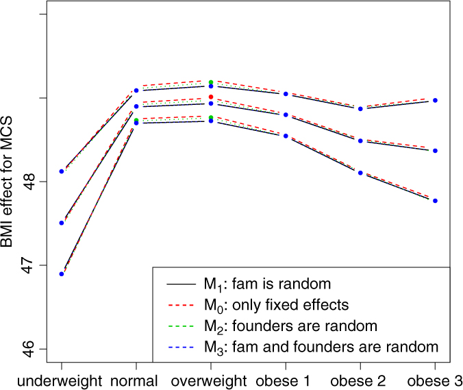
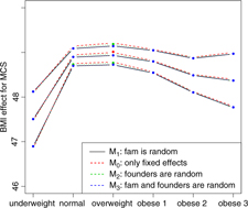
Fig. 2. BMI effects for MCS surrounded by confidence intervals.

Fig. 3. BMI effects for PCS surrounded by confidence intervals.
Table 4. Conditional F Tests for BMI, Age, and Sex of Selected Models

Figures 2 and 3 show the effect sizes of BMI (middle line) surrounded by confidence intervals (outer lines) of these effects. Plain lines are used for the selected models of MCS and PCS. Dashed lines are used for the other three models. Obviously, the effects of BMI on MCS and PCS of HRQoL match very closely across four models (lines overlap) and this is true for all categories of BMI. Confidence intervals also match very closely. This implies that the BMI effects do not change with and without accounting for relatedness in a family.
We see inverted parabolic shape of MCS across increasing BMI categories. A somewhat different shape is observed for PCS across increasing BMI categories. Interestingly, the MCS slightly increases for overweight people compared to the normal category. It also shows a dramatic drop for underweight individuals. The PCS decreases for all categories of BMI compared to the normal category, and the decreasing trend of PCS is increasingly steeper with increasing BMI. The confidence intervals of all BMI categories for PCS are beyond the confidence limits of the normal category, meaning that all BMI categories have substantially different PCSs than the normal category.
In Table 5, we present the coefficients for fixed effects with measures of uncertainty, namely standard error and lower and upper confidence limits. The results show that each additional year of age is associated with a 0.078-unit increase (0.1% of maximum observed value) in MCS and a decrease by about the same amount in PCS, on average, holding BMI and sex constant. Women have lower MCS, by approximately 1.891 units (2.6% of maximum observed value), and lower PCS, by approximately 1.011 units (1.4%), on average, holding BMI and age constant.
Table 5. Estimates of Coefficients for BMI, Age and Sex of Selected Models

Simulation Study: Design and Results
We conducted a simulation study to compare the commonly used variance component model with kinship matrix (Almasy & Blangero, Reference Almasy and Blangero1998) to our suggested model containing a reduced matrix of founders. The kinship model is computationally demanding and therefore we had to simulate relatively small sample sizes. We generated data using the model (10) shown below:
 $$\matrix{{{y_{ij}} = {\bf{x}}_{ij}^T\beta + {u_i} + {k_{ij}}\sigma _f^2 + {\varepsilon _{ij}},} \cr {{\varepsilon _{ij}}\mathop\sim\limits^{iid} N(0,\sigma _R^2),} \cr } $$
where definitions of xij, β, ui,  $\sigma _u^2$, $\sigma _R^2$ and ɛij are the same as in models (2), (3) and (4), $\sigma _f^2$ is the variance due to genetics and kij is the kinship effect for the jth member of the ith family. kij is generated from the multivariate normal distribution with mean zero and variance–covariance matrix Ω. The Ω consists of coefficients of pairwise relationships formed in the following way: in the first degree of relationship (parent–child and siblings), the coefficient of relationship is 1/2, in the second degree of relationship (grandparent/grandchild, half-sibling and avuncular), the coefficient of relationship is 1/4 and similarly for other degrees, as shown in Table 1 of Almasy and Blangero (Reference Almasy and Blangero2010). Technically, Ω is a block-diagonal matrix with coefficient of relationships among family members on the diagonal blocks and zeros (the coefficients of relationship between families) on the off-diagonal blocks.
Simulation parameters were selected from the results of the best-fitted model for Lifelines PCS data (see parameters in PCS: M3 of Table 5) and equal to: β underweight = 56.5, β normal = 57.5, β overweight = 56.7, β obese1 = 54.9, β obese2 = 53.0, β obese3 = 50.2, β age = −0.08, β sex = −1.0,  $\sigma _u^2 = 1.5,\,\sigma _f^2 = 6.0,\,\sigma _R^2 = 40.0$. The variable for age was generated from the normal distribution with a mean of 45 and a standard deviation of 14. The variable for sex was generated from Bernoulli distribution with a probability of .44 (for men). The number of observations for BMI categories ‘underweight’, ‘normal’, ‘overweight’, ‘obese 1’, ‘obese 2’, and ‘obese 3’ were generated from the multinomial distribution with probabilities of .007, .44, .401, .117, .026, and .009, respectively. These probabilities were calculated from the Lifelines data. Then the BMI was generated from a normal distribution based on the number of observations from the multinomial distribution and the following mean and standard deviation parameters: 17.7, 0.77 for ‘underweight’; 23.0, 1.5 for ‘normal’; 27.0, 1.4 for ‘overweight’; 32.0, 1.4 for ‘obese 1’; 37.0, 1.4 for ‘obese 2’; 43.0, 3.0 for ‘obese 3’. For family sizes, we set 2, 3, 4, 5 and 6 members, each size repeated 2, 4, 10, 20 and 38 times, respectively. Even though family sizes were repeated, in fact all families were different in their composition (e.g., for a family size of 2, we constructed parent–child and partner–partner families; for a size of 3, we constructed families of parent–parent–child, parent–child–grandchild, parent–child–child and parent–child–partner of child). In total, 74 families were constructed containing 384 numbers of observations. The PCS outcomes were generated using model (10). Afterwards, we fitted both models (kinship and M3) and compared the biases of heritability estimates and coverage probabilities of 95% confidence intervals of heritabilities. The heritability in model (10) is equivalent to hereditary ICC (h 2) and computed as shown in (7). Confidence intervals for heritability were calculated using the beta-approach, as described in Section 2.5. We conducted 100 simulations. The kinship model was fitted using the lmekin function of the coxme (Therneau, Reference Therneau2018) package and model M3 using the lme function of the nlme (Pinheiro et al., Reference Pinheiro, Bates, DebRoy and Sarkar2017) package in R. Results of the simulation studies are summarized in Table 6.
Table 6. Comparison of Heritability Parameters and Computational Time between Kinship (lmekin Function) and M3 (lme Function) Models

a Heritability is equivalent to hereditary ICC (h2) and computed using formula (7).
Results from setting 3 are shown in Figure 4. The kinship model results in larger bias (0.18) in comparison with the one (0.09) in M3 model. The M3 model results in larger variation than the kinship model on average, as shown in Figure 4. Subsequently, the kinship model demonstrates substantial undercoverage (0.86) while the M3 model shows some overcoverage (0.98) for a two-sided 95% confidence interval.

Fig. 4. Overlapping histograms for comparison of estimated heritabilities across M3 and kinship models in setting 3: vertical bar (0.13) shows true heritability, light grey histogram (left) and smoothed plain line show distribution of estimated heritabilities in M3 model and dark grey histogram (right) and smoothed dashed line show distribution of estimated heritabilities in kinship model.
We compared the computational time needed for fitting the kinship and M3 models. We varied the number of families and, correspondingly, the total number of observations. We examined three settings, each with 100 simulations. Settings and results are shown in Table 6. M3 is 8 times faster than the kinship model (setting 1). As the number of families quadruples (from setting 1 to 3), the computational time increases 2.5 times for the M3 model (lme function) and 15.2 times for the kinship model (lmekin function). Thus, there is an exponential increase in computational time for the kinship model as the number of observations increases while there is much slower increase (roughly linear) in computational time for the M3 model.
Discussion
In this study, the primary goal was to answer whether relatedness in a family must be accounted for when estimating the effects of risk factors of interest in large family-based cohort studies. The answer to this question is of particular importance for researchers analyzing the Lifelines data and data from other large cohort studies of families. From our study, it is clear that the effects of BMI on MCS and PCS of HRQoL scores do not change when accounting for family structure. This conclusion confirms theoretical considerations within longitudinal data analysis given by Diggle et al. (Reference Diggle, Heagerty, Liang and Zeger2002, chapter 1). The authors state that when the focus of the study is on modeling the dependence between the response and explanatory variable, then the nature of correlation among responses is unimportant if there is a large number of families relative to the number of individuals per family. Our Lifelines data clearly satisfy this criterion.
McArdle et al. (Reference McArdle, O’Connell, Pollin, Baumgarten, Shuldiner, Peyser and Mitchell2007) conducted a simulation study with the objective to compare the performance of association analysis of family-based designs that account for and ignore family structure in assessment of the phenotype–genotype association. They concluded that effect size estimates and power are not significantly affected by ignoring family structure, although type 1 error rates increase when family structure is ignored, and the magnitude of the increase depends on trait heritability and pedigree configuration. Induced type 1 error is directly related to diminished standard errors (and narrow confidence intervals), leading to liberal inference about regression coefficients, that is, falsely claiming significance when there is none. In our analysis of both PCS and MCS, we saw that ignoring the correlation (or family structure) led instead to larger standard errors of the regression coefficients (although the increase was very small), thereby leading to conservative inference about the covariate effects. Therefore, the standard errors of regression parameters can be larger or smaller when ignoring family structure, and therefore may lead not only to liberal inference and inflated type I errors, but also to conservative inference and deflated type I errors. Increase or decrease of the standard errors depends on (1) the relationship between the family structure and the covariates of interest and (2) the family structure effect size on the outcome.
We compared the Lifelines analysis results on association between BMI and HRQoL with similar results in the literature. Increased BMI has been shown to be associated with reduced physical HRQoL (Ul-Haq et al., Reference Ul-Haq, Mackay, Fenwick and Pell2012, Reference Ul-Haq, Mackay, Fenwick and Pell2013); however, evidence on the relationship between BMI and mental HRQoL was antagonistic. In the Lifelines study, we see reduced mental HRQoL for all categories of BMI in comparison with the overweight category. This conclusion matches with the conclusion of Ul-Haq et al. (Reference Ul-Haq, Mackay, Fenwick and Pell2013) from meta-analysis study. Furthermore, an inverted U-shape of mental HRQoL across increasing BMI categories is seen in both our Lifelines study (Figure 2) and that of Scottish study conducted by Ul-Haq et al. (Reference Ul-Haq, Mackay, Fenwick and Pell2012). Similarly to Ul-Haq et al. (Reference Ul-Haq, Mackay, Fenwick and Pell2013), we see that increasing BMI is associated with impaired HRQoL in Lifelines. In addition, our study reveals a shape of association between BMI and physical HRQoL. There is an inverted J-shape negative association in PCS across increasing BMI categories (Figure 3).
In this work, we studied real data and did not assume any a priori family inheritance structure. The main strength of our study is the use of Lifelines data which makes it possible to estimate the relatedness in more complex families than other studies can. Consequently, our results are practically more relevant. We learned that with or without accounting for family structure, the effect of determinants on health outcomes does not significantly change. Nevertheless, the ability to incorporate a family structure into our model in a computationally efficient way allows one to disentangle the genetic, shared behavioral and environmental variances. Furthermore, our proposed model allows for estimating hereditary, behavioral and shared environmental, and unique environmental ICCs of both HRQoL outcomes in computationally an efficient way through fractional relatedness of founders and non-founders.
The kinship model as implemented in the SOLAR (Almasy & Blangero, Reference Almasy and Blangero1998) software is unable to handle the analysis of the Lifelines data with over 89,000 individuals, although we did not study exhaustively all methods, such as generalized estimating equations (Liang & Zeger, Reference Liang and Zeger1986) that could have been used to implement the kinship model. We overcame the computational infeasibility with the kinship model by introducing and fitting a variance component model with fractional relatedness using standard functions in R.
We have made the assumption in our study that founders are unrelated, but Lifelines may not have complete information. For example, siblings’ information itself is not recorded within Lifelines, and therefore siblings might be modeled as two founders while they do have a common ancestor and are related. It would be interesting to examine whether modeling just a subset of founders would impact the variance component parameter estimates.
Furthermore, MCS and PCS may be genetically correlated, meaning that there is genetic overlap between these two traits (i.e., the same set of genes may regulate these traits). If interest lies in separation of genetic and environmental contributions simultaneously in MCS and PCS, then bivariate models could be used, similarly to the way that others (Lichtenstein et al., Reference Lichtenstein, Yip, Björk, Pawitan, Cannon, Sullivan and Hultman2009; Yip et al., Reference Yip, Björk, Lichtenstein, Hultman and Pawitan2008) modeled schizophrenia and bipolar disorder using multivariate generalized linear mixed models.
In summary, the proposed model offers to solve the computational issues involved in modeling family structure when thousands of families are analyzed, and subsequently to fit the model accurately using standard functions of R.
Acknowledgments
The authors wish to acknowledge the services of the Lifelines cohort study, the contributing research centers delivering data to Lifelines and all the study participants. The authors declare no conflicts of interest.
Financial support
During the first six months, this work was supported by the University of Groningen, University Medical Center Groningen as part of PhD thesis and later, it was supported by a NWO STAR travel grant from the University of Groningen. For the remaining work, this research received no specific grant from any funding agency, commercial or not-for-profit sectors.


 Open access