


1. INTRODUCTION
Engineering design practices the progression of an idea or conceptualization to a deliverable product. The premise is that a specific function, with defined performance parameters, must be married with a form to produce a product (Pahl & Beitz, Reference Pahl and Beitz1961). The delivered product expresses the bounding requirements of the design by correlating the original function to the performance of the final form through a prescribed cognitive process. Experience, from which creativity stems, provides the limits of the design space (Lopez et al., Reference Lopez, Linsey and Smith2011). Suboptimal design may occur when engineers fixate on domain-specific definitions of functions and potential solutions (Linsey et al., Reference Linsey, Tseng, Fu, Cagan, Wood and Schunn2010). Interdisciplinary options and experiences provide alternative solutions, but can fail to convey the idea of functionality or application due to differences of vocabulary, taxonomies, or methodologies.
Because there is merit to increasing design domains through analogies, this research provides quantitative options to incorporate controls engineering designs to the existing analogical approaches of mechanical engineering design (Linsey et al., Reference Linsey, Tseng, Fu, Cagan, Wood and Schunn2010, Reference Linsey, Markman and Wood2012; Lopez et al., Reference Lopez, Linsey and Smith2011; Fu, Chan, et al., Reference Fu, Chan, Cagan, Kotovsky, Schunn and Wood2013). The use of performance metrics and critical functionality through a function structure in a design space may correlate transfer functions with mathematics to produce analogies (Lucero, Reference Lucero2014; Lucero et al., Reference Lucero, Linsey and Turner2016). This research seeks to provide the initial frameworks of the matching techniques available to produce such analogies from control systems to engineering design.
More specifically, this research attempts to show the following:
-
1. A gap exists in functional representations of consumer products for mechanical engineering students with signal flows. This deficiency of signal flows may relate to energy and material flows acting as “carrier” flows for signals.
-
2. Usability of the schematic and numerical techniques already employed by controls systems engineering with transfer functions have similarities and applications to engineering design. By focusing on key performance parameters (KPPs) of a system, a translation to the engineering design domain is possible and can partially fill the signals gap.
-
3. There are several similarities and correlations between the two domains outlined herein that provide translations of ideas and product decompositions with the current domain practices: schematic similarities, performance matching through flows, mathematical function creation using bond graphs, and isomorphic matching of the aforementioned characteristics allows for analogical solutions.
2. ENGINEERING DESIGN AND RELATED WORK
Kleer and Brown (Reference de Kleer and Brown1984) provide a devise-based ontology to model the functionality of a system with black boxes of inputs and outputs. The function-behavior-state model developed by Gero (Reference Gero1990) and the function-environment-behavior-structure models (Deng et al., Reference Deng, Tor and Britton1999, Reference Deng, Britton and Tor2000; Deng, Reference Deng2002) operate as environment-centric viewpoints in function representations of the system. These models utilize functions as the effect an object has on the environment, and relate to the flows as the conduits of this change. These approaches rely on the engineer to provide the abstraction in the development of the system.
When seeking analogies appropriate for the design process, it is not uncommon to search for previous products. Short of maintaining and establishing independent repositories, the function-behavior-physical-effect-structure (Qian & Gero, Reference Qian and Gero1996) searches patents to provide analogies based on textual descriptions (Gero, Reference Gero1990). The structure, being the final configuration of the product, uses mathematical models like physical effect to show the state transition. Patent search tools circumvent the use of official repositories and have been researched as potential opportunities for analogies (Montecchi & Russo, Reference Montecchi and Russo2011; Russo, Reference Russo2012; Russo & Rizzi, Reference Russo and Rizzi2014). By utilizing the patent database, matching via graphical mapping is achievable and can pull from many domains. While these searches provide solutions from various sources, the applicability and functionality to the sourced target is left without context.
Design repositories established by various institutions and/or corporations have sought to capture product functionality and modeling. The National Institute of Standards and Technology established the Core Product Model, encompassing the standard functional basis (FB) taxonomy (Fenves, Reference Fenves2002). The Design Study Library, a biologically inspired design library, encourages analogical design through biological sources (Goel & Bhatta, Reference Goel and Bhatta2004; Goel et al., Reference Goel, Zhang, Wiltgen, Zhang, Vattam and Yen2015). The structure, behavior, and function modeling language attempts to provide a programming language capable of automating product teleology (Goel et al., Reference Goel, Rugaber and Vattam2009). However this automation seems to restrict the complete abstraction of the designer. The graphical modeling language, Systems Modeling Language (SysML), has been incorporated into a behavior library at a high-level representation (Kruse et al., Reference Kruse, Munzer, Wolkl, Canedo and Shea2012, Reference Kruse, Gilz, Shea and Eigner2014; Kruse & Shea, Reference Kruse and Shea2016). Yet many of these databases or repositories are independently operated and do not necessarily support collaboration.
Nagel (Reference Nagel2007) and Nagel et al. (Reference Nagel, Vucovich, Stone and McAdams2008) made efforts to move the FB taxonomy to a formal functional basis modeling language. Focusing on the signal flows, it is suggested that using a definitive grammar set improves communication between domains. While these rules are beneficial, they have yet to be enacted entirely with the FB taxonomy. The function-based systems engineering methodology implements functional modeling through product planning, conceptual design, and embodiment design phases (Hutcheson et al., Reference Hutcheson, Ryan, McAdams, Stone and Tumer2007). Hutcheson et al.’s work defines a behavioral model as a mathematical model of a system representing the ability to meet the requirements, complete with state variables. A conceptual behavior model enacts a behavioral model, free of the final form, of the product solution. Both the behavioral models and conceptual behavior models tie back to the requirements for full system traceability, yet remains at the systems engineering level.
Popular in systems engineering, a model-based systems engineering (MBSE) follows the standard systems engineering design process. SysML supports the MBSE approach via nine diagrams with a standard taxonomy (Friedenthal et al., Reference Friedenthal, Moore and Steiner2012, Reference Friedenthal, Moore, Steiner, Friedenthal, Moore and Steiner2015). The activity diagrams show the behavior of the product with inputs, outputs, and controls in a sequential fashion. The internal block diagram provides the interfaces and connections between the parts of a block. Still, no single diagram quantitatively encompasses the flows of a model, nor are there established relationships between the diagrams specifically for signals (Hampson, Reference Hampson2015).
Data flow diagrams are graphical representations of information systems via the inputs and output flows of data (Bruza & van der Weide, Reference Bruza, van der Weide and Prakash1989). Also known as “bubble diagrams,” data flow diagrams show the path of the data flow, but does not show processes, their sequences, nor process timing (Jayaram, Reference Jayaram2002; Jayaram et al., Reference Jayaram, Chen and Xi2003). These are powerful graphics showing the information only of the system, but fail to show full functionality with the collective flows of the system. In addition, they have yet to be fully adopted in mechanical engineering applications.
Several authors (Bracewell et al., Reference Bracewell, Bradley, Chaplin, Langdon and Sharpe1993, Reference Bracewell, Shea, Langdon, Blessing and Clarkson2001; Wu et al., Reference Wu, Campbell and Fernández2008; Kypuros, Reference Kypuros2013) suggest bond graphs as a means of producing analogies. Many authors have pointed out that bond graphs only apply to the energy flows and are not appropriate for signal flow as bond graphs work solely for energy. Nevertheless, it is possible to circumvent this issue by using the functionality of the bond graph components and adding nondimensional analysis to handle the signal flows.
A previous attempt to apply functional decomposition to mechatronics by Yuan and Ljung (Reference Yuan and Ljung2016) suggests that a combination of bottom-up, physical effect, and top-down decomposition approaches may be more effective than only a top-down decomposition approach. This research focuses on matching functions, but does not treat flows with the same attention. Cao et al. (Reference Cao, Liu and Paredis2011) highlight the issues of SysML to handle dynamic behavior or continuous dynamics in their models. In the same vein, Wu et al. (Reference Wu, Campbell and Fernández2008) show the strength of bond graphs in dynamic systems.
While there have been outstanding efforts to incorporate the ideas of functional modeling at a systems level with methods such as MBSE and SysML, complex domains such as mechatronics underutilize the potentials of analogies in developing product solutions. The functional modeling of engineering design and the schematic representations of controls systems proffer an opportunity to leverage the dissemination of information (via flows) mathematically to produce analogical solutions. The efforts of this current research seek to provide a bridge between these two domains and establish a framework for translation of information.
2.1. Functional representation
Product representation of individual functionality and the intermediary processes assists in product decomposition. Pictorial and matrix representations of the product behavior are common in understanding the sequence of events and the performance of the product. Function structures graphically depict individual, sequential functions of the product in operation. Disassembly of the overall functionality introduces a level of abstraction into the design process. The form of the final product is then heavily dependent upon the overarching performance required (Pahl & Beitz, Reference Pahl and Beitz1961). To use the function structure process, the system functionality must be broken down into individual purposes or subfunctions. Each subfunction is a box containing a “verb + noun” description representing the purpose with input and output flows. The input and output flows are nouns in the form of an energy, material, or signal wherein a flow acts upon as a verb.
The input and output flows are a manner of accounting for the physical system. Thermodynamically, the inputs must equate to the outputs regardless of the action occurring in the function box. The material flows follow the zeroth law of thermodynamics by again equating the input material to the output material despite the function acting on them, such as mass. The energy follows the first law of thermodynamics where all energy entering a system must exit it as well in the law of conservation of energy (Sonntag et al., Reference Sonntag, Borgnakke and Van Wylen2002). The signal flow does not flow a separate thermodynamic law, but rather is a combination of laws zero and one and is not conserved (Pahl & Beitz, Reference Pahl and Beitz1961; Sonntag et al., Reference Sonntag, Borgnakke and Van Wylen2002).
Otto and Wood (Reference Otto and Wood2001) propose a taxonomy that links multiple engineering disciplines and applications via the FB. The verb–object combination correlates to the function-flow of the individual functions to aide functional modeling methods by utilizing a generic level of specificity and synonyms. This research employs the FB as the cornerstone of functional modeling and assumes that the vocabulary is comprehensive and adequate for all engineering disciplines.
2.2. Domain specificity
Previous functional models maintain a focus on the representation of electromechanical consumer products. Many of the available examples in the literature and on the Internet focus on these small consumer products. The FB now caters to the representation of these types of devices. Based upon a review of functional models by the authors (Lucero et al., Reference Lucero, Viswanathan, Linsey and Turner2014), a typical model consists of approximately 10 flows and perhaps 20 functions. Of these flows, approximately 90% represent energy or material flows, while only 10% represent signal flows. A sample taken by the authors of functional models from design textbooks and the Oregon State Design Repository, encompassing 40 functional models, indicates that 40% of flows represent material flows, 49% of flows represent energy flows, and 11% represent signal flows. Similarly, the 20 models extracted from design textbooks included approximately twice the number of unique flows as those that were present in the repository, suggesting more thorough modeling of the flows from the design textbooks than those within the repository. These models showed a similar dominance of material (40%) and energy flows (51%) in comparison to signal flows (9%). Neither textbook models nor those generated from design activities in the repository appear to include significant signal flows. In a reverse engineering context, these flows are often difficult to identify, but for forward design problems, signal flows are a critical element in the design of the system controller.
Signal flows are not independent of material or energy flows, as the signal flows require a carrier flow (in the form of an energy or material flow) to exist. Therefore, signal flows can never be more than 50% of all flows. The low percentage of signal flows is also indicative of the products typically modeled via this approach, and is likely the result of the clear majority of available functional models representing reverse engineered systems. Most electromechanical consumer products include limited instrumentation and control systems, and therefore involve significant signal pathways, such as that which may occur with a rudimentary control system. Yet many systems of interest from a modeling standpoint, whether abstracted to a functional level, represented with a bond graph model of dynamic behaviors, or represented with a controls block diagram model, exhibit a much more exhaustive signal flow network representation than is typically modeled functionally. A functional model often abstracts the inner workings of a control system into a small set of highly abstracted functions with limited signal modeling included. This is particularly true if the subject of the model is the result of a reverse engineering exercise whereby the signals intended by the design are not necessarily obvious during reverse engineering. Nonetheless, the result is an abstracted functional model with limited signal domain contributions.
The resulting “signal gap” in functional models does present a significant impact upon the design of systems. Without a model of the signals involved in the system, the control system for the design becomes a time-intensive post hoc process. Coupling control system design with the physical system design could reduce downstream modifications to the physical system and may dramatically improve the performance of the control system and the system.
2.3. Design by analogy
Analogies can offer alternative solutions to design problems. They provide engineers with analogical solutions based on a linguistic or visual portrayal of the design problem and description. Visual analogies increase innovation of the design solution for both novice and expert engineers (Casakin et al., Reference Casakin, Goldschmidt and Planning1999). However, experimental results show that experts employ more analogies than novices employ and in a more creative fashion (Ball et al., Reference Ball, Ormerod and Morley2004). Where the novices flock to analogies that closely resemble their current design problem, the experts draw from numerous examples that can offer partial analogies and various design domains.
Because there is merit to increasing design domains through analogies, this research provides quantitative options to incorporate controls for engineering designs to the existing analogical approaches (Lopez et al., Reference Lopez, Linsey and Smith2011; Linsey et al., Reference Linsey, Markman and Wood2012; Fu, Murphy, et al., Reference Fu, Murphy, Yang, Kevin, Jensen and Wood2013). The use of performance metrics and critical functionality to model a function structure in a design space may correlate transfer functions with mathematics to produce analogies (Lucero, Reference Lucero2014; Lucero et al., Reference Lucero, Linsey and Turner2016). This research seeks to provide the initial frameworks of the matching techniques available to produce such analogies.
2.4. Bond graphs
Bond graphs, like block diagrams, allow for pictorial representations of systems, but also allow for dynamic scaling from component to full system via the energy in the system as seen in Table 1 (Karnopp et al., Reference Karnopp, Margolis and Rosenberg1990; Borutzky, Reference Borutzky2010; Kypuros, Reference Kypuros2013). A pictorial representation of a graph with nodes and edges displays the system as a network. Each of the nodes is a port of energy (dE/dt) or power exchange, called a “power port,” which acts as an intersection for the subsystems (Borutzky, Reference Borutzky2010). The edges are connections between two nodes relaying information about the type of power transferred.
Table 1. Control system through and across variables correlated to bond graph variables.

Since bond graphs are a method of translating system functionality with a defined set of components using power, the physical process of action on the power must occur with two quantities: effort and flow. The effort and flow variables are domain dependent, but when multiplied together, result in power in standard units. In addition to effort and flow, there are two other categories of use in bond graphs, momentum and displacement, which categorize the type of system represented. In dynamic systems, the energy changes over time while using the momentum and displacement variables as the energy variables to account for the time fluctuation. The combination of these variables allows for a specific definition of the bond graph components as seen in Table 2.
Table 2. Bond graph components and their mathematical relationships to bond graph effort and flows

3. CONTROLS ENGINEERING
Controls engineering is a multidisciplinary engineering domain encompassing such factions as mechanical, electrical, and software engineering. The premise of controls engineering is to quantify the performance of a system and is common in robotic, computer visualization, mechatronic, and manufacturing applications (Mayr, Reference Mayr1970; Karayanakis, Reference Karayanakis1995; Dorf & Bishop, Reference Dorf and Bishop1998; Doyle et al., Reference Doyle, Francis and Tannenbaum1990; Åström & Kumar, Reference Åström and Kumar2014). Controls engineering is the basis for feedback theory and linear system analysis, melding together communications theory and network theory into a singular methodology to track and alter system response. Control theory deigns performance objectives are baselined via quantitative analysis by using these controls metrics in specifications and design definitions.
As with the typical engineering design process, the preliminary steps of control theory start with an identification of, and the means to measure, the overarching system's functionality. In the case of control theory, the “control” of the identified parameter will be the focus of the remaining study, usually with some level of accuracy entrenched in the parameter definition. With the specified accuracy, sensors monitor the parameter to measure the control variable. Depending on the definition of the problem, the final architecture of the control system (i.e., open or closed loop, robustness, signal sensitivities, etc.) can be considered.
Open control-loop systems, such as extrusion-based additive manufacturing, run through the desired process without gauging the progress of the designed function. Thus, with additive manufacturing cases, a part can fail due to thermal or structural stresses while continuing the build process in a catastrophic manner, resulting in the “rats' nest” conundrum. “Open loop control systems employ an actuating device to control the process directly without using feedback,” whereas “a closed loop system uses a measure of the output and feedback of the signal to compare with the desired output (reference or command)” (Dorf & Bishop, Reference Dorf and Bishop1998). Closed-loop systems provide feedback as to the status of the operations and allow for alterations of some control to guide the desired outcome. Examples of closed-loop systems are residential thermostats, Crockpots, or soldering irons as simple tools. The efforts of this current research focus on the open-loop system, but intentions to handle closed-loop systems exist.
A control system shows the interfaces and interactions of individual components to produce a desired system response. Analysis of the system response comes from the linear system theory where a system assumes a cause and effect relationship. Like the black box models of engineering design, the cause and effect are synonymous with inputs, outputs, and processes. There is a relationship established between the input and output streams based upon the processes performed, providing the cause and effect on the signal. The graphical representation of control theory via the block diagrams is akin to the function structures of engineering design by using transfer functions to provide the mathematical representation of the processes.
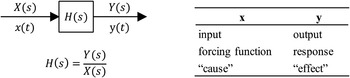
Fig. 1. Generic block diagram with system inputs and outputs, including mathematical representation.
3.1. Transfer functions
Transfer functions represent the system variables and dynamic relationships of signals. For linear and linear approximations of systems, the transfer functions are the ratio of the Laplace transform of the output variable to the Laplace transformation of the input variable where all initial conditions are zero (Fig. 1). The Laplace transform translates the inputs/outputs from the time domain into the frequency domain through a process H(s) shown in Eq. (1):
 $$H\lpar s \rpar = \displaystyle{{{Y}\lpar s \rpar } \over {X\lpar s \rpar }}.$$
The developed transfer function equation compares the input parameter to the output parameter via through variables and across variables of individual components operating as a system (Borutzky, Reference Borutzky2010; Kypuros, Reference Kypuros2013). Like bond graphs with efforts and flows, the variables define the ability to carry a flow. For example, current (dimensional analysis theory [DAT] units; DAT L3T–1) is a through variable in an electrical system with transfer functions, whereas it is a flow in bond graph terminology. The across variable is the voltage potential (DAT units ML−1T−2), which is equivalent to a bond graph effort. When multiplied together, the voltage and current (or effort and flow) produce power (DAT units ML–2T–3). Thus, the focal point of the system is the energy and power of the system, in the same manner as bond graphs (Table 3).
Table 3. Control system and bond graph nomenclature comparison converging on the shared power and energy terms

4. TRANSLATING TRANSFER FUNCTIONS TO ENGINEERING DESIGN
This section provides the initial framework for connecting the controls systems and engineering design domains as a cohesive methodology. Utilizing the FB and the design-by-analogy framework, we suggest that four methods exist for engineers to use in comparing designs:
-
1. Schematic similarities: control system block diagrams ≈ function structures of functional modeling
-
2. Quantifiable performance metrics: control variables of control systems ≈ nondimensional flows of the FB.
-
3. Mathematical functions: Control system differential equations of transfer functions ≈ FB flows as defined by bond graph characteristics
-
4. Isomorphic matching: Identifies analogical alternatives by matching the DAT units and bond graph component similarities
We work through each step of the approach using an example problem of a direct current (DC) motor. From the DC motor example problem, we continue to additional examples that are more scalable in the next section with more comprehensive discussions.
4.1. Schematic similarities
This work previously identified gaps in the signal flows of the FB in functional decomposition. While present in many systems and products, these flows rarely appear in the function structures developed by mechanical engineering students. Exploiting the field of controls engineering may increase the appearance of signal flows in function structures. The block diagrams utilized in control systems proffer similar graphical representation of functional modeling with verb + noun combinations of the FB in function structures in the block diagrams. Since controls engineering does not use a specified taxonomy, there is not a perfect one-to-one translation between the two domains. However, the block diagrams utilize mathematical functions, via differential equations, which show the same cause–effect relationships between the control variables and verbs (actions) as seen in the FB.
Controls engineering relies heavily on the reduction of block diagrams to simplified diagrams based upon feedback techniques (Fig. 2). This research does not establish relationships to the reduction or simplification techniques, but instead proposes that the graphical similarities are still applicable regardless of the block diagram complexities. Using the blocks as the intersections of functions, the interconnecting flows are traced though the system with emphasis placed on the signal flows, regardless of the system complexity.

Fig. 2. Control engineering system depictions: (a) black box model of process to be controlled, (b) open-loop control system with no feedback, and (c) closed-loop feedback control system to provide actual output.
These schematic similarities are akin to the work outlined by Gentner (Gentner & Gentner, Reference Gentner and Gentner1982; Gentner, Reference Gentner1983), where the use of conceptual relations or specific operations can span across various domains to describe functionality. For example, Gentner and Gentner (Reference Gentner and Gentner1982) found electricity to be analogous to “flowing” mechanisms such as flow within pipes. While the flow of electrons is not exactly like the flow of a water molecule in a pipe, it is an analogy between two complex systems, describing how to achieve some action. Thus, the relational structure of how an action is similar yet unbound by the object or domain of origin.
The block diagrams of controls engineering allow for sequential mathematical relationships to be developed based upon this cause-effect method, which is similar in sequential product depiction to the functional modeling. The how portion of an action is depicted in the block diagram mathematically while the function structure shows the systems-level analysis of what is done linguistically. Thus, there is no direct translation between the two domains, but parallels exist from the graphical representations of the product system. Note that controls engineering can still provide how the process occurs. For example, monitoring the amplification signal from an op-amp or Wheat-stone bridge circuit conveys how much amplification is occurring in the system.
The block diagrams consist of unidirectional, operational blocks representing the transfer function on the input and output variables. Block diagrams have the cause–effect relationship allowing for the tracking of specific control variables, such as those of the signal flows of the FB. Like function structures, the operational blocks can have multiple inputs and output for a multivariable control system. Likewise, actions occurring on the flows result in the cause and effect mentioned previously.
Example
A DC motor is a power actuator device, delivering energy to a load as resistively shown in Figure 3a and as physically sketched in Figure 3b. The DC motor “converts” DC electrical energy to rotational mechanical energy. The armature generates the torque of the system (via the rotor windings and stator windings), which drives an external load. DC motors have many applications in disciplines such as power systems, robotics, and mechatronics. The example given is adapted from Dorf and Bishop (Reference Dorf and Bishop1998). ■
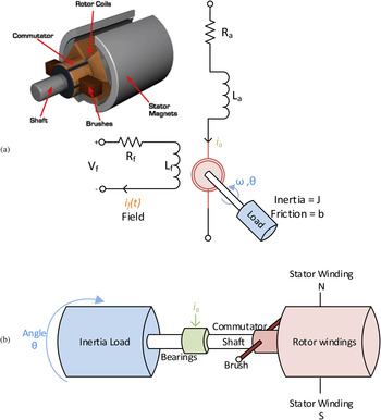
Fig. 3. (a) Electrical schematic of a motor for voltage applied across the field and (b) physical representation of the electrical schematic.
4.2. Quantifiable performance metrics
All engineering design problems revolve around KPPs, which are the overarching target functionality of the system or product. Previous work in quantifying the performance of these KPPs, and mapping them to flows of the FB, has established frameworks in technical engineering variables with corresponding units (Lucero et al., Reference Lucero, Linsey and Turner2016). The FB flows are characterizations of their respective material, energy, or signal flow, which can be further decomposed into their secondary levels showing more specificity, allowing for the establishment of the individual flows capable of measurement via sensors. For example, a material flow for a fluid physical system could be the volumetric flow rate (DAT units L3T–1) of some working fluid as measured via flowmeters such as pitot-tubes or ultrasonic Doppler flow meters.
The DAT provides a relationship between physical quantities as defined by their fundamental dimensions of length, mass, time, charge, temperature, and luminosity (White, Reference White2003). Through combinations of these base units, it is possible to produce almost any engineering flow, but with a reduced number of variables. This dimensional homogeneity allows for: the reduction of the number of variables in a system, fundamental modeling of physical relationships of the entire system, and scalability of models through the set number of relevant control variables.
Previous research by Coatanéa (Reference Coatanéa2005) and Lucero et al. (Reference Lucero, Linsey and Turner2016) has established the use of the DAT parameters for engineering design using flow parameters. By correlating the flows to these DAT parameters, it is possible to match the nondimensional units based on the exponential power of the dimensionless units present. This change therefore can be accounted for via a transfer function that compares the output to input parameters to identify which action was performed on the flows by equating the exponential power of the input and output flows. For example, integrating angular acceleration (DAT units T–2) with respect to time (DAT units T), results in angular velocity (DAT units T–1).
If using the power (DAT units ML2L–3) or energy (DAT units ML2L–2) of a system as the performance parameter, it becomes easy to translate across domains, as these parameters do not alter. The method of obtaining the power might be different per domain, but the result of the parameter is the same with DAT units ML2L–3. For example, multiplying voltage by current equates to electrical power in the electrical domain while in the thermal heat transfer domain, the temperature multiplied by the entropy flow rate defines thermal power. This manner of comparing exponents for the power and energy parameters allows for the transition between domains via bond graph variable combinations for power and energy variables as shown in Table 4 for selective domains.
Example
When employing the FB, the statement of work for the DC motor is “convert electrical energy to mechanical (rotational) energy” as shown in Figure 4a. The input into the system is electrical energy in the form of voltage (DAT units ML–1T–2), while the output is mechanical (rotational) energy via torque (τ; DAT units ML2T–2) and rotational velocity (ω; DAT units of degree T–1), waste energy in the form of Watts (DAT units ML2T–3), and rotational position (degrees θ). The function structure of the KPP remains at a systems-level depiction where the mechanisms by which the conversion of the energy is ambiguous. The black box representation merely looks at the inputs to outputs and allows the DAT units to be the performance parameters quantified in the system. ■
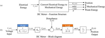
Fig. 4. (a) Direct current motor function structure per the functional basis and (b) controls system block diagram for the energy flows as outlines in (a).
Table 4. Functional basis functions categorized into bond graph components based upon functionality characteristics

However, the controls block diagram for the DC motor (Fig. 4b) with the method of conversion defined, established a transfer function for this specific system wherein the position is the signal to be monitored. A linear approximation of the actual motor develops from the input voltage to the output position, while neglecting second-order effects (i.e., hysteresis and voltage drop across the brushes). Thus, using sequential differential equations, the final positional displacement (degrees θ) is calculated.
4.3. Mathematical functions
Functions, within the FB, are the performance of an action on the flows. These actions correlate to the active characteristics of bond graph components and can be thus categorized per Table 4. With the five bond graph components, engineers can seek mathematical relationships using transfer functions as a ratio of the output to input flows via Laplacian transforms [Eq. (1)]. There can be many mathematical possibilities for each of the bond graph components, but this method establishes the mathematical baselines.
From these characteristic baselines of each component then, it is possible to quantify the action modeled. For example, a regulate function, acts a resistive element that can show the level of efficiency across the input and output streams. This behavior provides quantitative bounds in performance metric analogy searches. In so classifying the behavior of the resistive element, it is possible to look at any of the similarly classified functions as a starting point. Thus, the mathematical relationships between the inputs, outputs, and actions ensuing give additional opportunities to search for analogies based upon similar functionality.
Ideally, a repository of the all the mathematical functions associated with each bond graph component would be established. For algorithmic analogy programs, such as D-APPS (Lucero, Reference Lucero2014), it would be possible to have a database of target analogies that exhibit mathematical relationships similar to those of the source (transfer function). More specifically, the transfer functions provide a quantitative solution which can bound the range of the performance metrics sought (i.e., “seek a resistive element that only allows 180° of rotation).
Example
In the DC motor control system, the performance parameters are the voltage, torque, and rotational velocity. The field terminals have an applied constant current to operate. Assuming a linear relationship with the torque and the air gap flux of the motor as shown in Eq. (2).
 $$T_m = K_1K_{\rm f}i_{\rm f}\lpar t \rpar i_{\rm a}\lpar t \rpar \comma \,$$
where i f(t) is the field current and K represents various constants. ■
The field current motor provides power amplification, which allows Eq. (2) to be written in the Laplace transform notation of Eq. (3), where the constant armature current (i a) is equivalent to I a.
 $$T_{\rm m}\lpar s \rpar = (K_1K_{\rm f}I_{\rm a})I_{\rm f}\lpar s \rpar = K_{\rm m}I_{\rm f}\lpar s \rpar. $$
Equation (4) defines the input voltage of the field as a function of the motor inductance and resistance.
 $$V_{\rm f}\lpar s \rpar = \lpar {R_{\rm f} + L_{\rm f}s} \rpar I_{\rm f}\lpar s \rpar .$$
The motor torque [T m(s)] of Eq. (5) is the total torque delivered to the load as functions of the load torque [TL(s)] and the disturbance torque [T d(s)]. It is common to assume T d(s) is negligible and to define T L(s) as shown in Eq. (6).
 $$T_{\rm m}\lpar s \rpar = T_{\rm L}\lpar s \rpar R + T_{\rm d}\lpar s \rpar \comma \,$$
 $$T_{\rm L}\lpar s \rpar = Js^2{\rm \theta} \lpar s \rpar + bs{\rm \theta} \lpar s \rpar .$$
For T L(s) and T m(s) in Eqs. (7)–(8), rearrange Eqs. (3)–(6) and introduce I f(s) as Eq. (9).
 $$T_{\rm L}\lpar s \rpar = T_{\rm m}\lpar s \rpar + T_{\rm d}\lpar s \rpar \comma \,$$
 $$T_{\rm m}\lpar s \rpar = K_{\rm m}I_{\rm f}\lpar s \rpar \comma \,$$
 $$I_{\rm f}\lpar s \rpar = \displaystyle{{V_{\rm f}\lpar s \rpar } \over {R_{\rm f} + L_{\rm f}s}}.$$
Equation (10) relates rotation to voltage via the transfer function of the output over the input.
 $$\displaystyle{{{\rm \theta} \lpar s \rpar } \over {V_{\rm f}\lpar s \rpar }} = \displaystyle{{K_{\rm m}} \over {s\lpar {Js + b} \rpar \lpar {L_{\rm f}s + R_{\rm f}} \rpar }}I_{\rm f}\lpar s \rpar = \displaystyle{{V_{\rm f}\lpar s \rpar } \over {R_{\rm f} + L_{\rm f}s}}.$$
This final transfer functions equation relates back to the FB through the performance metrics and the bond graphs. The flow streams match to DAT unit parameters, as modeled by the input/output streams. Once identified, these flows cross the system boundary as the transfer function of Eq. (10) and match to the convert function of the FB to provide characterization of the action. Note that the bond graph components characterize the action (Table 4) and thus allow for any gyrator component functions to be considered.
4.4. Isomorphic matching
As the schematic similarities (Section 4.1) outlined, the graphical representations of the control-system block diagrams and those of the function structures offer opportunities to traverse engineering domains through pictorial representations of system functionality. However, the analogy identification occurs in this current step where computer matching can identify analogical solutions with similar functionality and comparable performance metrics (via DAT). Using graph theory as outlined in D-APPS (Lucero, Reference Lucero2014), the functions (mathematical or verbs alike) become the nodes of a design space, while the flows (DAT units) become the connections between the nodes (Gould, 2014). Thus, the functions are equivalent to nodes in a design space with interconnections of edges (or vertexes). The edges, with their exponential DAT units of the performance parameter, can then relay upon the mathematical functions (Section 4.3) to find similarities to other functions or bond graph component types.
The engineering performance parameters can traverse domains by matching the DAT exponents. Treating the flows with their dimensionless units as the inputs and outputs of a black box, the function, or action, enacted upon the flows provides the mathematical operation by numerically comparing the input to output unit exponents. These actions become the ratio of the output to input of transfer functions and produce a mathematical relationship for each specific flow conversion. Thus, if laid in the graphical representation of graph theory, the functions are the nodes, while the flows are the edges or interconnections between the nodes. This representation provides the foundation for the mathematical functions and quantification of the performance parameters.
Isomorphic matching compares the nodes and edges of the source against a target. D-APPS employs this isomorphic matching to determine how similar a target function structure is to various analogous functions structures (Lucero, Reference Lucero2014). By incorporating the control systems block diagrams into a graphical design space, tools such as D-APPS can perform the isomorphic matching to determine how close potential solutions can be to the target problem. Consequently, the matching efforts become a graphing problem wherein the various nodal and vertex combinations are the basis for combinations and permutations capable of analysis.
After review of the function and bond graph characterizations for many systems, it may be possible to build a repository quantifying the actions of the functions through the functional categories outlined in Table 4. Similarly, mapping the dimensionless flows of the FB to the transfer function intermediary variables enables comparison of the actions in the black box on the exponential units. Opportunities are now available to seek analogies within specific signal flows using both functionality and quantifiable performance metrics.
Example
The DC motor signal flow identified as a KPP was the rotational position. Building a graph of the convert function and the other flows, the figure in Figure 5a is possible with the DAT versions of each performance parameter. Referring to the bond graph component groupings (Table 4), the convert function acts like a gyrator wherein an effort is converted to a flow or vice versa. Per this grouping, the convert and control magnitude functions have similar functionality and can be possible analogies. ■

Fig. 5. (a) Simplified graph of the direct current motor with performance parameters, (b) graph of a gyroscope, and (c) comparison graph of the direct current motor and the gyroscope, showing potential analogy identification. Working back from the rotational position, the gyroscope functions.
A gyroscope is a component commonly used in aerospace applications in attitude determination and control efforts. It is a device of a wheel or a disk mounted in gimbals, rapidly spinning about an axis leveraging the angular momentum of this spin to alter or maintain the direction of the tilt (Mcbride & Cellier, Reference Mcbride and Cellier2001). The control magnitude function then is the critical function acting to alter the torque to rotational velocity and position (Fig. 5b). Since both the DC motor and the gyroscope signal flow of rotational position are the output parameter, the analogy can be drawn as Figure 5c, where the difference between the input flows is identified as the delta of the exponential components.
This correlation of matching is done using critical functionality (bond graph component grouping) and performance parameters (DAT). With the transfer function established from the DC motor, it would be further possible to quantify the extent of the rotational position achieved with this specific example. Thus, we are not suggesting that a gyroscope is a replacement for a DC motor, but that the method of sensing the rotational position has parallels that need further investigation from the engineer.
5. EXAMPLE PROBLEMS
The following two examples demonstrate the ability to traverse domains using the methodology discussed previously. Demonstrated with different levels of complexity and process transparency, the two example problems include their function structures, block diagrams, and the transfer functions with suggested analogies. The first problem works through a hot glue gun, where the key functionality is to extrude melted glue at a controlled flow rate with basic transfer functions. The second problem shows the applications of a more complex system with a biological sensor application by providing the basis for the graphical similarities and quantification. Each example is simply a proof-of-concept validation, and much like engineering design, proffers a single solution among many.
5.1. Hot glue gun
A hot glue gun operates by melting glue sticks via a heating element and extruding the melted glue through the nozzle through the actuation of a trigger. The heating element uses electricity and a voltage regulator to control the amount of heat added to the system as required per the material characteristics of the glue sticks, which is dependent upon the melting point of the sticks. The glue gun trigger controls the flow rate of the melted glue as actuated from the hand-held force applied. Releasing the trigger halts the extrusion, but the thermal regulator maintains the required temperature to keep the stick melted. This example emphasizes the signal controls process for regulating the temperature through the conversion of electrical energy to heat energy.
The function structure displays the signal flows, in orange arrows, indicating the controlling paths of the temperature and the glue flow rate (Fig. 6). The KPP of the system, “maintain the temperature of the glue gun,” leads to the identification of two critical pairs: convert electrical energy to heat energy and regulate melted glue flow. Sensors control the energy and material flows in the system through control loops and allow for the signals flows to be highlighted in this example.

Fig. 6. (a) Function structure of hot glue gun, and (b) control system block diagram of glue gun operation for a closed-loop system.
The control block diagram of the glue gun lays out the process by which the energy and material is sensed, and controlled by the glue gun electricity regulator. However, the control system does not perform the entire systems analysis like the functional modeling but instead focuses on the signal mechanisms. In this manner, the control block diagram shows similar graphical characteristics as the function structure, but is only applicable to the signal mechanism by providing the “how” the heating is controlled. The temperature of the glue gun can be decomposed into nondimensional temperature units (θ) and traced through the closed-loop system.
The heat addition to the system is
 $$\displaystyle{{\Theta \lpar s \rpar } \over {q\lpar s \rpar }} = \displaystyle{1 \over {C_{\rm t} \times s + (Q \times S + 1/R_{\rm t})}}\comma \,$$
where Θ is Θgun – Θ0, which is the temperature difference due to the thermal process; C t is the thermal capacitance; Q is the fluid flow rate or constant; S is the specific heat of air; R t is the thermal resistance; and q(s) is the transform of rate of heat flow of heating element.
Assuming an addition of unit step q(s) = 1/s to alter the temperature, the response of the system becomes
 $${\rm \tau} \lpar s \rpar = \displaystyle{{1/C_{\rm t}} \over {s + \displaystyle{{QS + 1/R} \over {C_{\rm t}}}}} \times \displaystyle{1 \over s} = \displaystyle{{\rm \beta} \over {s + {\rm \alpha}}} \times \displaystyle{1 \over s} = \displaystyle{{ - {\rm \beta} /{\rm \alpha}} \over {s + {\rm \alpha}}} + \displaystyle{{{\rm \beta} /{\rm \alpha}} \over s}\comma \,$$
where α = (QS + 1/R)/C t and β = 1/C t.
Taking the inverse Laplace transform yields
 $${\rm \tau} \lpar t \rpar = \displaystyle{{ - {\rm \beta}} \over {\rm \alpha}} e^{ - {\rm \alpha t}} + \displaystyle{{\rm \beta} \over {\rm \alpha}} = \displaystyle{{\rm \beta} \over {\rm \alpha}} [ {1 - e^{ - {\rm \alpha t}}} ] .$$
Assuming steady state conditions where the temperature of the glue gun remains constant for melting the glue stick once the desired temperature is reached, the time approaches infinity (t → ∞) leading to
 $${\rm \tau} \lpar t \rpar \to \displaystyle{{\rm \beta} \over {\rm \alpha}} = \displaystyle{1 \over {Qs + 1/R}}.$$
Using the KPP of the hot glue gun, the flows can be nondimensionalized for both the electrical energy and the temperature, providing the correlation between the function structure and control system diagrams as seen in Figure 7. The transfer function allows for the quantification of these flows as performance metrics for the system while the function structure provides the linguistic representation of the system. In this fashion, the performance metrics and the critical function convert represented in tandem with bond graphs to provide alternative approaches to altering electrical energy to a temperature.
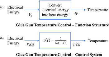
Fig. 7. Key performance parameters for (a) a function structure of hot glue gun and (b) a control system block diagram of glue gun operation for a closed-loop system.
As an analogy example, consider a hair blow dryer (Fig. 8). The glue gun isomorphic graph (Fig. 8a) shows the regulation of electrical energy to a temperature through a control magnitude function. By comparison, the blow dryer regulates the temperature and air flow rate. However, for this example, we are concerned with the temperature only and how the temperature is sensed to generate feedback within the system. Because both the control magnitude and regulate functions are considered resistive bond graph elements, it is possible to consider the output performance parameter of temperature as a potential functional analogy for the system (Fig. 8c).
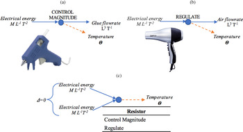
Fig. 8. Potential analogy for sensing the temperature of (a) a glue gun and (b) a hair dryer using their key performance parameters. (c) The analogy can be achieved via isomorphic matching of the bond graph component (resistive) and the exponential values of the nondimensionalized units.
Much like the DC motor example presented previous, the premise behind analogy mapping is not a one-to-one match providing “how” to utilize the analogy. Instead, this lays out a method for potential analogies based upon the performance metrics and functionality. How the analogy will be applicable to the design engineers is up to them consider the context of their problem and what portions of any analogy could be useful to them.
5.2. Saccadic eye movement sensors
A saccade is a jerky movement of the human eye to adjust its focus from one target to another. With reaction times of approximately 50 ms for a 10° saccade, the human eye muscles are among the fastest reacting muscles in the human body (Enderle & Bronzino, Reference Enderle, Bronzino and Bronzino2012). These movements are useful when the eyes are locating a target using accurate, but jerky, motion and without care of the information moving across the retina during the movement. A saccade turns the visual system off until it is complete. After the saccade, the system operates in a closed-loop mode to verify that the target is now in view. Use of information from the retinal view of the new scene and muscle proprioceptors aides the correction for any errors between the current and desired eye position.
A typical experimental protocol for observing saccades has the subject seated before a light-emitting diode (LED) target display. The subject must maintain focus on the lit LED, move their eyes as fast as possible, and avoid false tracking. The experimenter switches power from one LED to another LED, which changes the optical signal. This optical signal converts to electrochemical neural responses in the brain. The brain must fire the muscles attached to the eyeball by converting the electrochemical neural signal into mechanical activation of the appropriate muscles. The mechanical contraction of the muscle of the eye results in a rotation of the eyeball, resulting in a saccade, which is the process of focus in this example.
From the vantage point of the experimenter, the objective is to measure the speed and reaction time of the human eye with respect to a change in the stimulus signal as a position. The KPP of the system is then “measure the position of the eye after the stimulus triggers.” Therefore, the key flows to track are the eye itself (Fig. 9a), the object providing the stimulus signal (Fig. 10), and the device(s) used to track the movement of the eye (Fig. 11a,b). While each of these flows can decompose into its own independent function structure, it is important for the experimenter to define the function of the protocol for the experiment (Fig. 12). For the experimenter, the objective is to collect data for comparison to his or her model (Fig. 9b) of human eye motion. The experimenter needs to account for the function of the experimental apparatus and whether it will provide the data for comparison to the experimenter's equations for motion [Eq. (15)–(21)] of the eyeball.

Fig. 9. (a) Muscle anatomy of the ocular motor system and (b) the corresponding Westheimer second-order mechanical eye model.

Fig. 10. Example light-emitting diode board to provoke a horizontal saccade eye movement.

Fig. 11. (a) Depicted for the right eye, a scleral search coil measures eye movement via coils embedded into either a fitted contact lens or a rubber ring that adheres to the eye. Magnetic fields, from magnets around the eye, generate electric currents in the search coils. By measuring the variations in polarity and amplitude of the current generated from the angular displacement of the eye, the position of the eye can be determined. (b) Fixed infrared light emitter(s), directed at the eye, will reflect an amount of infrared light to the fixed receiver(s), which will vary per the eye's position.
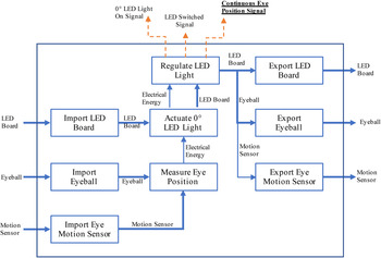
Fig. 12. Example function structure for the saccadic eye movement sensor.
In 1954, Westheimer published an eye model (Fig. 9b) for describing horizontal saccades in response to a 20° target displacement (Westheimer, Reference Westheimer1954). The Laplace variable analysis provides the mathematical expression
 $$J{\rm \ddot \theta} + B{\rm \dot \theta} + {K \theta} = {\rm \tau} \lpar t \rpar .$$
Assuming 0° for initial eye orientation, the standard form of the transfer function for Eq. (15) is
 $$\eqalign{ H\lpar s \rpar=\displaystyle{{Y\lpar s \rpar } \over {X\lpar s \rpar }} = \displaystyle{{\rm \theta} \over {\rm \tau}} = \displaystyle{1 \over {Js^2 + Bs + ({ K )}}} = \displaystyle{{{\rm \omega} _n^2 \lpar {s^2 + 2{\rm \zeta} {\rm \omega}_{\rm n}s + {\rm \omega}_{\rm n}^2} \rpar } \over {K}}\comma \,} $$
and for a 20° saccade,
 $${\rm \omega} _n = \sqrt {\displaystyle{{K} \over J}} 120\comma \,$$
 $${\rm \zeta} = \displaystyle{B \over {2\sqrt {{K} J}}} = 0.7\comma \,$$
where B is the frictional rotational element, J is the moment of inertia, and K is the stiffness.
The torque, τ(t), generated by the lateral and medial rectus muscles evokes the saccade and a new eye position, θ(t). Per Westheimer's data (Westheimer, Reference Westheimer1954), the roots of the transfer function are complex and given as
 $$s_{1\comma 2} = {\rm \zeta} {\rm \omega} _{\rm n} \pm j{\rm \omega} _{\rm n}\sqrt {1 - {\rm \zeta} ^2} = - 84 \pm j85.7.$$
Assuming a step input for the system, ${\rm \tau} \lpar s \rpar = \displaystyle{{\rm \gamma} / s}$
, the new eye orientation, θ(t), becomes
${\rm \tau} \lpar s \rpar = \displaystyle{{\rm \gamma} / s}$
, the new eye orientation, θ(t), becomes
 $${\rm \theta} \lpar t \rpar = \displaystyle{{\rm \gamma} \over {K}}\bigg[ {1 + \displaystyle{{e^{ - {\rm \zeta} {\rm \omega}_nt}} \over {\sqrt {1 - {\rm \zeta}^2}}} \hbox{cos}\left( {{\rm \omega}_n\sqrt {1 - {\rm \zeta}^2} t + {\rm \psi}} \right)} \bigg]\comma \,$$
where
 $${\rm \psi} = {\rm \pi} + \hbox{ta}\hbox{n}^{ - 1}\displaystyle{{ - {\rm \zeta}} \over {\sqrt {1 - {\rm \zeta} ^2}}}. $$
This experiment, when broached from the engineering design perspective, allows for tracking the saccade in multiple ways. Two example methods of eye motion tracking are the employment of a scleral (Fig. 11a) search coil and infrared oculography (Fig. 11b). These motion-tracking methods share the same function structure for understanding human ocular mechanics work, but leave the how the tracking is done up to the designer. DAT, with bond graph theory, makes it possible to compare the search coil method to the oculography method as they have equivalent functionality (measure) and KPP (eye rotational position).
A scleral search coil measures eye movement via coils embedded into either a fitted contact lens or a rubber ring that adheres to the eye where a wire leaves the eye at the temporal canthus (Fig. 11a). For horizontal saccade experiments, two inducting coils placed on either side of the head produce magnetic fields. During saccade eye movement, the scleral coil will move, which causes fluctuations in the magnetic fields. The new orientation of the eye is determined by measuring the variations in the polarity and amplitude of the magnetic field caused by the angular displacement of the scleral coil. The input is the position of the eyeball and the output is the change in the magnetic field.
Infrared oculography uses a fixed infrared light source directed at the eye (Fig. 11b). The amount of infrared light reflected to a fixed detector varies with the eye's position. The infrared transmitters and receivers mount to frames for eyeglasses, and as infrared light is invisible to the eye, it does not serve as a distraction to the subject. In addition, the ambient lighting level of most facilities does not affect measurements because infrared detectors do not detect these light sources. The input of this system is the position of the eyeball and the output is the change in the infrared radiation detected.
We can use DAT and bond graphs to construct the relationship between these two methods. In terms of bond graphs, both systems relate the change in the eyeball angle through a flux linkage. The movement of the eyeball changes the position and orientation of the scleral coil, resulting in a flux in the magnetic field. Similarly, the change in the position and orientation of the eyeball produces a flux in the infrared light detected. Thus, the two solutions presented in Figure 12 are functionally analogous in their approach to measure the eye saccade, but vary solely in implementation.
6. CONCLUSIONS
Engineering design has sought to produce practices that allow for abstraction in the final design. Functional modeling methods, such as the FB, establish uniformity of the cognition process for the mechanical domain with material and energy flows. However, there is a deficit in the use and approach to the signal flows as evidence by the teaching of functional modeling to mechanical engineering students using consumer products.
Because of this gap, the research herein attempted to find approaches upon which methods and processes from other engineering domains could provide more examples. The authors suggest utilizing controls engineering to bridge the gap to provide both similar graphical representations and mathematical potentials. Comparing the block diagram used to track and “control” the variables of the system to the function structures of the FB identifies functional similarities. Establishing linear, differential equations for products is possible when concurrently using the block diagrams and the relationships between the inputs, outputs, and actions of the system.
Some of the outcomes of this research include the following:
-
• Current functional modeling pedagogy lacks robust examples of signal flows when looking at functional representations of consumer products with mechanical engineering students. This deficiency in signal flows may relate to energy and material flows carrying the signal flows.
-
• Schematic similarities between functional modeling techniques, particularly the function structures, and the control-system block diagrams allow for translations between domains. The graphical representation of the system models are not identical matches, but functions and flows correlate through the energy and power variables of bond graphs.
-
• Quantifying the KPPs of a system is possible for system performance metrics using DAT, such as Buckingham-Pi. The energy and power variables of bond graphs allow the translation of the DAT units of the FB flows and the control variables of control systems.
-
• The functions of the FB equate to transfer functions of control systems through bond graph component behavioral functionality. The five components of bond graphs (resistive, capacitive, inductive, transformer, and gyrator) have specific behavioral characteristics defined by the interactions of the performance parameters. When seeking functional analogies, these characteristic groups are the basis for the isomorphic matching.
-
• Design-by-analogy options are available to fill the signal flow gap by utilizing the bond graphs and block diagrams of control systems via isomorphic matching. Treating the functions (via the proposed bond graph component grouping) as the nodes and the flows (via the DAT unit exponentials) as the edges, comparisons between individual components is possible for analogical similarities.
-
• Applying the proposed methodology to problems of various complexities and scales is feasible due to the use of DAT. Three example products represent the domain agnostic application of the developed theories and provide evidence of this methodology.
This research is in the preliminary stages and requires further verification and validation. Additional analysis from student populations will provide the applied basis for these processes. It is necessary to develop this concept of relating controls engineering with engineering design based upon additional data collection, repository comparisons, and example problems. This framework may allow inclusion of analogies stemming from more engineering domains and not just those of mechanical or electrical domains.
Briana M. Lucero is an R&D Engineer in the Advanced Engineering Technologies Division at Los Alamos National Laboratory. She holds a bachelor's degree in engineering (mechanical and electrical specialties), a master's degree in mechanical engineering, a master's degree in systems engineering from Johns Hopkins University, and a doctoral degree in engineering systems from Colorado School of Mines. Briana's current research is on modeling and simulation of tools in additive manufacturing. Dr. Lucero worked on satellites and scientific imaging instrumentation as an Aerospace Engineer at Ball Aerospace and Technologies Corporation and Los Alamos National Laboratory. That work informed her use of systems engineering.
Matthew J. Adams is a PhD student in biological design at Arizona State University. He is also a Co-Founder of the health systems engineering company Kintel, LLC. Matt received his BS degree in physics from the University of Maryland, College Park, and his MS degree in mechanical engineering from the Colorado School of Mines. He currently holds student memberships in both ASME and the Orthopedic Research Society.
Cameron J. Turner is a Professor in the Department of Mechanical Engineering at Clemson University. He previously worked at the Colorado School of Mines and was also a Technical Staff Member at Los Alamos National Laboratories. Dr. Turner teaches classes in engineering design methods, design optimization, mechanical systems, computer-aided design/engineering/manufacturing, and design of complex systems. Cameron is currently the Program Chair for the ASME CIE Division Executive Committee and is a member of the International Design Simulation Competition Committee of ASME. Prof. Turner won the CSM Design Program Director's Award in 2015 for service to the capstone design program.


