


1. Introduction
Glide-snow avalanches, also known as full-depth or glide avalanches, are a type of snow avalanche that release directly on the ground. They can therefore be massive and threaten infrastructure such as roads, houses and ski-lift masts in alpine regions (Stimberis and Rubin, Reference Stimberis and Rubin2011; Techel and others, Reference Techel, Pielmeier, Darms, Teich and Margreth2013; Humstad and others, Reference Humstad, Venås, Dahle, Orset and Skrede2016). Mitigation of glide-snow avalanches is challenging, however, because traditional control techniques such as explosives are ineffective (Clarke and McClung, Reference Clarke and McClung1999; Sharaf and others, Reference Sharaf, Glude and Janes2008; Simenhois and Birkeland, Reference Simenhois and Birkeland2010). Additionally, forecasting capabilities are poor (Jones, Reference Jones2004; Reardon and others, Reference Reardon, Fagre and Lundy2006; Simenhois and Birkeland, Reference Simenhois and Birkeland2010; Höller, Reference Höller2014) due to a limited understanding of the underlying processes.
Currently, snow gliding is thought to require a slope angle of more than 15 degrees, a bed surface with low roughness and liquid water between the ground and snowpack (Gand and Zupančič, Reference Gand and Zupančič1966). Of these three requirements, the presence of liquid water at the ground–snow interface is considered the key for understanding and predicting glide-snow avalanches (Clarke and McClung, Reference Clarke and McClung1999; Jones, Reference Jones2004; Höller, Reference Höller2014; Ancey and Bain, Reference Ancey and Bain2015). Although the importance of this interfacial water is widely accepted, few studies have addressed the detailed dynamics of its formation. In early field observations, the presence of interfacial water during glide events was simply noted (Eugster, Reference Eugster1938; Bucher, Reference Bucher1948; Gand and Zupančič, Reference Gand and Zupančič1966). Later, field experiments measured increases in glide velocity with rain or meltwater at the ground–snow interface (McClung, Reference McClung1975; Stimberis and Rubin, Reference Stimberis and Rubin2011) and concluded that the presence of an interfacial slush layer (approximately 6–14 vol% liquid water content) formed favorable conditions for gliding (Clarke and McClung, Reference Clarke and McClung1999). Clarke and McClung (Reference Clarke and McClung1999) hypothesized that interfacial water comes from two sources. In so-called ‘warm-temperature’ events, water is generated at the snow surface (surface melting or rain) and percolates to the ground, while in ‘cold-temperature’ events, interfacial water comes from the glide surface (soil, grass or rocks) through melting. Mitterer and Schweizer (Reference Mitterer and Schweizer2012) later added suction as a possible mechanism for interfacial water formation after observing brownish water at the base of glide-avalanche crowns. Mitterer and Schweizer (Reference Mitterer and Schweizer2012) hypothesized that this water was sucked into the snowpack from the ground and showed, through preliminary simulations, that the snowpack can generate sufficient capillary forces to do so. Recently, several studies have correlated increases in the liquid water content of the snowpack and soil near the soil–snow interface with glide events (Ceaglio and others, Reference Ceaglio2017; Fromm and others, Reference Fromm, Baumgärtner, Leitinger, Tasser and Höller2018; Maggioni and others, Reference Maggioni, Godone, Frigo and Freppaz2019). However, aside from Mitterer and Schweizer (Reference Mitterer and Schweizer2012), none of aforementioned studies addressed the detailed dynamics of interfacial water formation.
One reason for the limited number of studies on the detailed dynamics of interfacial water formation is the lack of suitable measurement techniques. An ideal measurement technique for studying the detailed dynamics of interfacial water formation is non-destructive, has a sufficiently high temporal resolution (seconds to minutes) and has a spatial resolution capable of capturing the ground–snow interface. On grassy slopes, grass under the snowpack is compressed to thicknesses of approximately 1–3 cm (Feistl and others, Reference Feistl, Bebi, Dreier, Hanewinkel and Bartelt2014), while the transition from soil to snow (without vegetation) or from rock slab to snow is even smaller. Thus, the required vertical spatial resolution to resolve dynamics within these thin interfacial layers is on the order of 1 mm.
Techniques for measuring the liquid water content of snow were reviewed in-depth by Kinar and Pomeroy (Reference Kinar and Pomeroy2015a). Manual techniques such as the hand-squeeze-test (Fierz and others, Reference Fierz2009), calorimetry (Kawashima and others, Reference Kawashima, Endo and Takeuchi1998), the Denoth meter (Denoth and others, Reference Denoth1984; Denoth, Reference Denoth1994) and the snow fork (Sihvola and Tiuri, Reference Sihvola and Tiuri1986) are destructive and/or prohibitively time-intensive for achieving high temporal resolutions since a user must make every measurement. Certain non-destructive techniques utilizing radar (Bradford and others, Reference Bradford, Harper and Brown2009; Heilig and others, Reference Heilig, Eisen and Schneebeli2010), acoustic signals (Kinar and Pomeroy, Reference Kinar and Pomeroy2015b), electrical self-potential (Kulessa and others, Reference Kulessa, Chandler, Revil and Essery2012; Priestley and others, Reference Priestley2022) and GPS (Koch and others, Reference Koch, Prasch, Schmid, Schweizer and Mauser2014) can measure continuously, but generally only provide bulk measurements. Other continuous, non-destructive techniques such as tensiometry (Colbeck, Reference Colbeck1976) and techniques utilizing dielectric permittivity (Schneebeli and others, Reference Schneebeli, Coléou, Touvier and Bernard1998; Ceaglio and others, Reference Ceaglio2017; Fromm and others, Reference Fromm, Baumgärtner, Leitinger, Tasser and Höller2018; Maggioni and others, Reference Maggioni, Godone, Frigo and Freppaz2019) provide higher vertical spatial resolutions down to a few centimeters (depending on the sensor), but only provide point measurements. It should be noted that while probe-based techniques are considered non-destructive, they necessarily disrupt the snow structure. The magnitude of this effect varies by device. The snow fork, for example, theoretically increases the density of the measured snow volume by 12.5% (Sihvola and Tiuri, Reference Sihvola and Tiuri1986), which affects the liquid water content measurement. More recently, magnetic resonance imaging (MRI) (Adachi and others, Reference Adachi, Yamaguchi, Ozeki and Kose2020; Katsushima and others, Reference Katsushima, Adachi, Yamaguchi, Ozeki and Kumakura2020), Raman spectroscopy (Maggiore and others, Reference Maggiore, Tommasini and Ossi2022) and near-infrared hyperspectral reflectance (Donahue and others, Reference Donahue, Skiles and Hammonds2022) were shown to provide non-destructive, high-resolution, liquid water content measurements. These techniques each have their own advantages and disadvantages. For example, the hyperspectral imaging by Donahue and others (Reference Donahue, Skiles and Hammonds2022) has relatively high spatial and temporal resolutions, but the signal is dominated from the scanned surface, which is sensitive to edge effects. Raman spectroscopy and MRI can also provide high spatial resolutions at the cost of temporal resolution.
Techniques for measuring the liquid water content of soil have also been extensively reviewed (Dobriyal and others, Reference Dobriyal, Qureshi, Badola and Hussain2012; Lekshmi and others, Reference Lekshmi, Singh and Baghini2014; Yu and others, Reference Yu2021). Several techniques such as ground-penetrating radar (Chanzy and others, Reference Chanzy, Tarussov, Bonn and Judge1996), time-domain reflectometry (Topp and others, Reference Topp, Davis and Annan1980; Topp and Davis, Reference Topp and Davis1985), capacitance measurements (Dean and others, Reference Dean, Bell and Baty1987), MRI (Amin and others, Reference Amin1996; Haber-Pohlmeier and others, Reference Haber-Pohlmeier, Caterina, Blümich and Pohlmeier2021) and tensiometry (Gardner and others, Reference Gardner, Israelsen, Edlefsen and Clyde1922; Richards and Gardner, Reference Richards and Gardner1936) have been used for both snow and soil with the same advantages and disadvantages discussed above. Other techniques such as gravimetry (Schmugge and others, Reference Schmugge, Jackson and McKim1980) are analogous to techniques used in snow (here, calorimetry). As with snow, probe-based devices in soil are disruptive (Rothe and others, Reference Rothe1997) and only provide point measurements. X-ray tomography provides non-destructive, high-resolution 3D images of the liquid water distribution within soil. When performed at a synchrotron X-ray source, the temporal resolution is now on the order of seconds (Tötzke and others, Reference Tötzke, Kardjilov, Manke and Oswald2017; Ferreira and others, Reference Ferreira, Pires and Reichardt2022).
At this time, none of the aforementioned techniques have been shown to provide the simultaneous, non-destructive, high-resolution, liquid water content measurements of soil, snow and the soil–snow interface necessary for unraveling the detailed dynamics of water transport across this interface. In this pilot study, we demonstrate the use of neutron radiography to image water transport in soil–snow systems. Columns of sand, gravel and snow were used to simulate the capillary forces of the soil–vegetation–snow layering found in nature. The columns were connected to a water reservoir to maintain a constant-pressure boundary condition and placed in a climatic chamber within the neutron beam. Melting experiments were performed. The technique provided non-destructive, 2D measurements at a spatial resolution below 100 μm and sub-minute temporal resolution. Due to the exploratory nature of these experiments, this paper has two goals. First, we provide the experimental methodology and image processing necessary for observing water transport processes with neutron radiography. Second, we provide results from two proof-of-concept experiments illustrating how the formation of liquid water layers in the basal snowpack can be imaged with this technique. Neutron radiography therefore shows promise for investigating the water transport across the soil–snow interface, which is relevant for fields such as glide-snow avalanche formation and hydrology.
2. Materials and methods
2.1. Column preparation
Samples were prepared in aluminum columns (14 × 14 × 2.5 cm3 outer dimensions and 0.25 cm wall thickness) connected to a water reservoir via a flexible plastic hose at the base of the column (Fig. 1). The columns were packed in two configurations simulating the capillary forces of the layering found in nature. One configuration simulated soil with an overlying snowpack and one configuration simulated soil, a vegetation layer (e.g. grass), and an overlying snowpack. Soil was simulated with sand (0.3–0.9 mm diameter) and vegetation was simulated with gravel (2.0–3.2 mm diameter). Fine-grained sand (0.06–0.25 mm diameter) was used in combination with gravel to form the lower boundary of the sand–snow and sand–gravel–snow configurations (Fig. 1). The sands (Carlo Bernasconi AG (Bern, Switzerland)) were immersed in water during packing. The fine-grained sand prevented air invasion, thereby maintaining the hydraulic connection between the water reservoir and the sand. The gravel layer at the bottom prevented the fine-grained sand from entering the plastic hose. A plastic tube with holes was inserted above the fine-grained sand to allow air to escape as the melted snow infiltrated into the sand and interface layers, which prevented ponding.

Figure 1. Schematic of the aluminum column and water reservoir (not to scale). The layering is representative of the experimental results presented in Figure 4. For the results shown in Figure 5, there was no gravel layer between the sand and snow. In both configurations, a vertical plastic tube with small holes was placed above the fine-grained (FG) sand layer to allow air to escape. The beam direction was perpendicular to the 14 × 14 cm2 face.
Once the sands were packed, the column was chilled to approximately 0 $^\circ$ C prior to packing of the snow. The snow was a natural snow sample of small rounded grains with a diameter of 0.25–0.75 mm, a density (before packing into the column) of 375 kg m−3 and a specific surface area of 10 m2 kg−1 (measured with IceCube (A2 Photonic Sensors, Grenoble, France)). Prior to packing, the snow was stored in a $-18\, ^\circ$
 C freezer. The snow was transferred into the column with a wooden spoon to minimize heat transfer. The density of the snow after packing was not measured and, due to repacking, could differ from the pre-packed value above (see below). The snow was packed within an insulated cooler that was pre-chilled (air temperature approximately $-5\, ^\circ$
 C).
C).
Once the column was packed and the open-beam images (with and without black-body grid) were taken, the column was transferred to the beamline in a cooler and loaded into the climatic chamber (at $-5\, ^\circ$ C). The water hose was fed through a hole in the bottom of the chamber and connected to the water reservoir located outside of the chamber. The hose was reattached such that no air bubbles were formed within the tubing. The water reservoir was placed at a height to induce a −6 cm pressure head in the middle of the sand layer. Once the column was in the chamber and connected to the water reservoir, imaging was started and the temperature of the climatic chamber increased to slightly above $0\, ^\circ$
 C to induce melting. This temperature varied based on the intended melting rate. The sample was oriented such that the beam direction was perpendicular to the 14 × 14 cm2 face (i.e. the neutrons passed through 2.5 cm of the column).
2.2. Neutron radiography
Neutron radiography experiments were performed on the NEUTRA beamline at the Swiss Spallation Neutron Source (SINQ) of the Paul Scherrer Institute (PSI) in Villigen, Switzerland. Samples were placed inside the climatic chamber described by Mannes and others (Reference Mannes, Schmid, Wehmann and Lehmann2017) within the beam. The climatic chamber has 15 cm × 15 cm × 15 cm internal dimensions with cooling and heating elements to regulate the temperature. The detector system was a 100 μm 6Li ZnS:Cu scintillator with an Andor iKon-L camera using a Zeiss Otus 55 mm f/1.4 lens. The pixel size was 84 μm. Images were taken every 30 s with 30 s exposure to the neutron beam. A grid of perfect neutron absorbers, black-bodies, were used to facilitate the scattering correction described below. Here, we used 10B 4C cylinders with a diameter of 2.5 mm and a thickness in the beam direction of 3 mm which were mounted in an aluminum grid at 25 mm center-to-center spacing (Carminati and others, Reference Carminati2019). The black-body grid is placed in front of the chamber.
2.3. Image processing
Image processing was performed using Python 3.8.3 and standard Python libraries. Radiography is based on the idealized Beer–Lambert law relating the measured intensity to the incoming beam intensity via

where I is in the intensity measured by the detector, I 0 is the incoming beam intensity before interacting with the sample, μ is the linear attenuation coefficient of the sample (depends on sample composition, density and neutron energy) and z is the path length through the sample (see schematic in Fig. 2). Importantly, the measured value I contains the effects of all system biases. These biases include the detector efficiency, dark current (detector noise), non-sample related attenuation, scattering and other effects which may be present depending on the specific system. The measured intensity must be corrected with the contributions of these biases in order to obtain meaningful results.

Figure 2. Schematic of radiography illustrating the components of Eqn (1).
To conceptually understand the correction (prior to the mathematics below), we first describe a few key terms, which are illustrated in Figure 3. The dark-current image represents the detector signal while the neutron beam is off (i.e. detector noise). The open-beam image (here, taken with the black-body grid) accounts for non-sample attenuation (here, the empty climatic chamber and black-body grid). The scattering contribution is calculated with the measured intensity behind a grid of perfectly absorbing black-bodies (described in detail below) (Carminati and others, Reference Carminati2019). Finally, dosis terms are used to account for fluctuations in the incoming neutron beam intensity. The contributions from the dark-current and scattering are subtracted from the measured image, which is then divided by the open-beam (also corrected for dark-current and scattering). This corrected image is then scaled by the dosis terms.
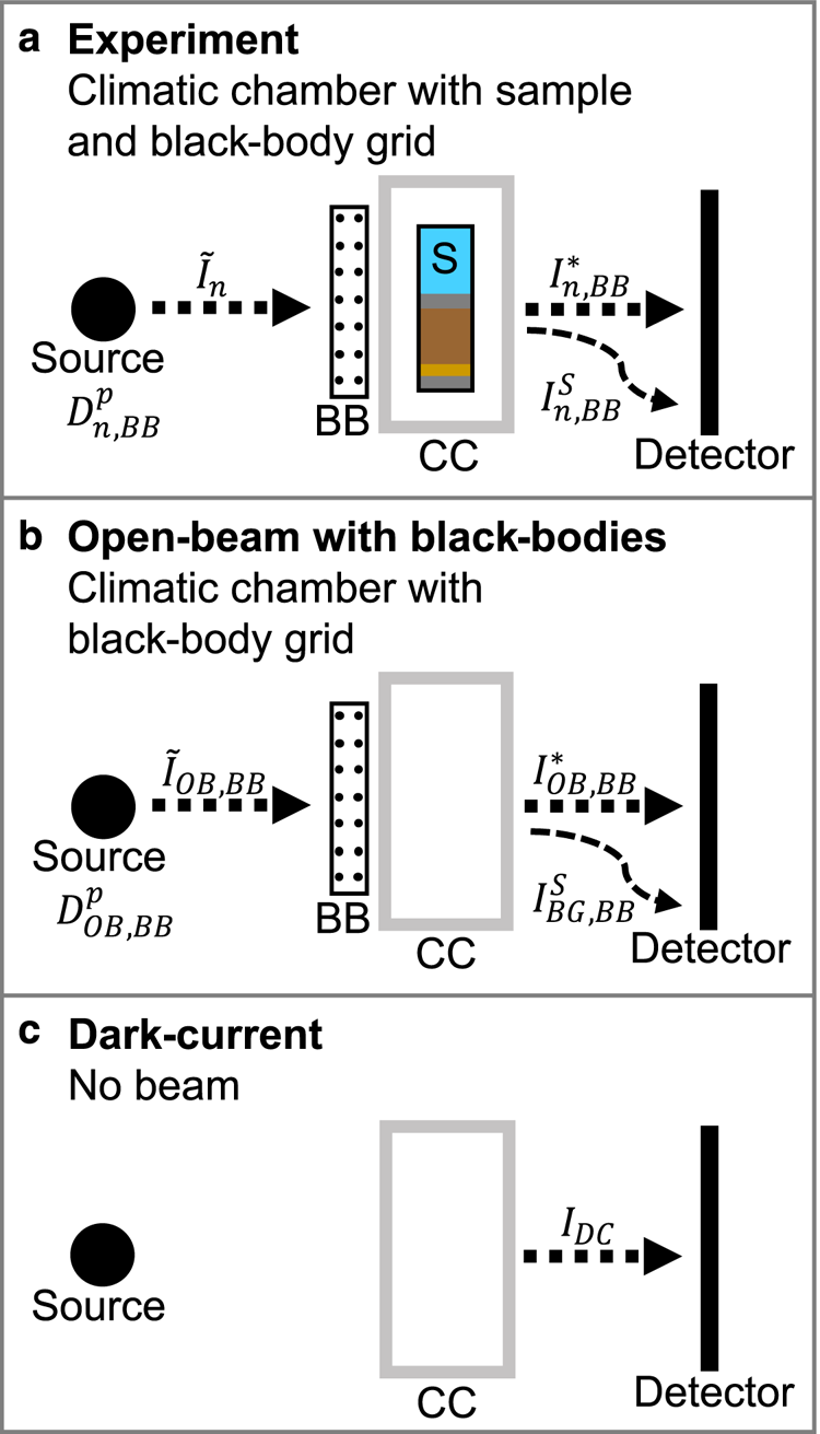
Figure 3. Schematic of the imaging configurations with the components of Eqn (5). The diagrams show the positions of the black-body grid (BB), climatic chamber (CC) and sample (S) for the different imaging configurations. The configuration in (a) was used for the experiments while the configurations in (b) and (c) were used to obtain values needed for the corrections in Eqn (5). The dosis terms ($D^p_{OB, BB}$ and $D^p_{n, BB}$
 ) represent fluctuations in the neutron source and the scattering terms ($I^S_{n, BB}$
 and $I^S_{BG, BB}$
 ) are calculated (not directly measured).
For these experiments, the black-body grid remained in place for the duration of each experiment. This allowed us to calculate the scattering contribution for every image, thereby maximizing the temporal resolution. This also allowed us to simplify the equations by Carminati and others (Reference Carminati2019) (note that we retain the original notation).
We begin with Eqn (2) (from Carminati and others (Reference Carminati2019))

where the dosis correction terms (Z n and Z OB) are given by


and $\widetilde {I}_{n}$ is the intensity corrected for beam fluctuations, $\widetilde {I}_{{\rm OB}}$
 is the open-beam intensity corrected for beam fluctuations, $I^\ast _{n}$
 is the measured intensity of the n th image, I DC is the dark-current, $I^\ast _{{\rm OB}}$
 is the open-beam image without black-body grid, $I^\ast _{{\rm OB, BB}}$
 is the open-beam image with black-body grid, $I^S_{n, {\rm BB}}$
 is the scattering contribution of the n th image with black-body grid, $I^S_{{\rm BG, BB}}$
 is the scattering contribution of the black-body grid, τ BB is a term accounting for the reduced beam intensity due to the black-body grid, and ‘D()’ indicates dosis terms accounting for variations in the incoming beam intensity.
To simplify Eqn (2), we first replace $I^\ast _n$ with $I^\ast _{n, {\rm BB}}$
 because we do not have any sample images without the black-body grid. We also replace $I^\ast _{{\rm OB}}$
 and $\widetilde {I}_{{\rm OB}}$
 with $I^\ast _{{\rm OB, BB}}$
 and $\widetilde {I}_{{\rm OB, BB}}$
 , respectively, because the open-beam image with black-body grid is now the relevant scaling quantity to calculate the transmission. We eliminate the dosis correction terms (Z n and Z OB) associated with the scattering images ($I^S_{n, {\rm BB}}$
 and $I^S_{{\rm BG, BB}}$
 ), respectively, because we are now dividing the measured sample image with black-body grid ($I^\ast _{{\rm n, BB}}$
 ) by the open-beam with black-body grid ($I^\ast _{{\rm OB, BB}}$
 ), which takes into account the attenuating effect of black-body grid. Finally, we replace the overall dosis correction terms ($D \left(I^\ast _{{\rm OB}} - I_{{\rm DC}} - I^S_{{\rm BG, BB}}Z_{{\rm OB}}\right)$
 and $D \left(I^\ast _{n} - I_{{\rm DC}} - I^S_{n, {\rm BB}} Z_{n} \right)$
 ) with the proton dosis of the open-beam images with black-body grid ($D^p_{{\rm OB, BB}}$
 ) and the sample images ($D^p_{n, {\rm BB}}$
 ), respectively. The proton dosis terms correct for fluctuations in the incoming neutron beam with the measured proton flux hitting the neutron-generating target. With these modifications, Eqn (2) is simplified to Eqn (5) (see Fig. 3 for an illustration of the terms).

Finally, we take the natural logarithm of both sides to obtain the unitless optical density (Eqn (6)).

For comparison to the Beer–Lambert law, we divide both sides of Eqn (1) by I 0 and take the natural logarithm, resulting in Eqn (7).

We now see that the left side of Eqn (6) is in the same form as the left side of Eqn (7) where $\widetilde {I}_{{\rm OB, BB}}$ is the effective incoming beam as it accounts for non-sample attenuation. The right side of Eqn (6) is therefore equal to μz, the unitless optical density. Note that an optical density of 0 corresponds to 100% transmission and positive optical densities correspond to transmission values less than 100%.
On the right side of Eqn (6), all quantities are measured except for the scattering images ($I^S_{n, {\rm BB}}$ and $I^S_{{\rm BG, BB}}$
 ). Scattering images were calculated as described in Carminati and others (Reference Carminati2019) using a thin-plate splines interpolation. Briefly, the intensity behind each black-body is assumed to be due only to scattering (perfect absorbers). Thus, interpolation between the black-bodies provides the scattering contribution for all pixels.
The median value of the open-beam with black-body grid (10 images), and dark-current (2 images) image sets was taken to obtain one image per set for the correction (e.g. for the open-beam images, the median value of the 10 images was taken for each pixel).
To generate vertical profiles, a region of interest (ROI) was selected (e.g. Figs 4a–f and 5a–f) and the average pixel value across the ROI at this height was used. The vertical profiles were smoothed with a Savitzky–Golay filter with a filter window of 11 and a 3rd order polynomial to reduce noise. For the generation of images in Figures 4a–f and 5a–f, negative values resulting from the correction in Eqn (5) were substituted with interpolated values (multivariate interpolation) to improve the visual clarity. For this reason, the optical densities of the black-bodies in Figures 4a–f and 5a–f are numerical artifacts from the correction process and should be ignored. Neither the interpolated nor negative values were used when calculating the mean for the profiles.
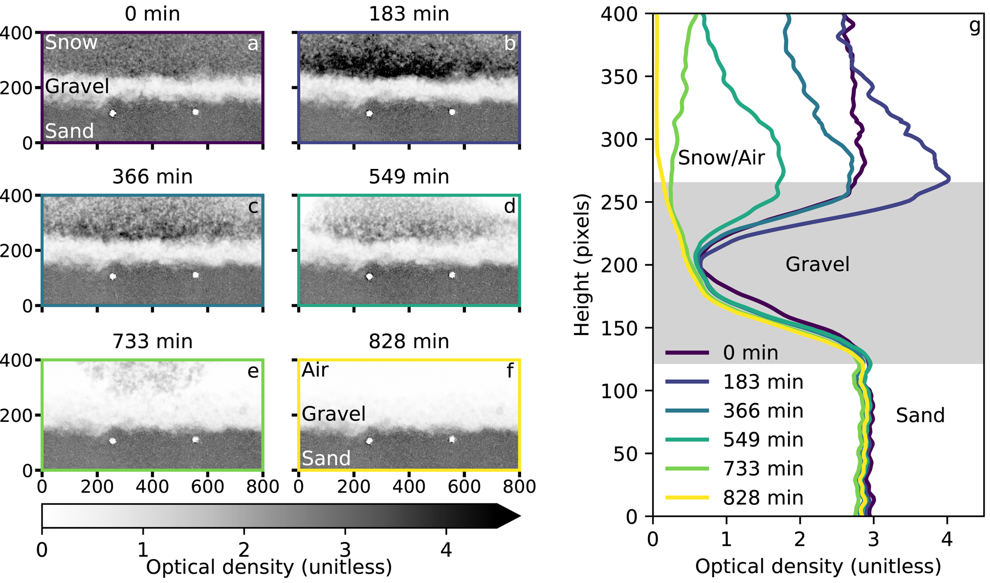
Figure 4. Results of an experiment with a gravel layer at the sand–snow interface showing a time series of images (a–f) and vertical profiles (g). Units of (a–f) are pixels with a pixel size of 84 μm. Each curve in (g) corresponds to an image in (a–f). The gray region in (g) shows the gravel interface including the sand–gravel and gravel–snow transition zones. The region above the gray band is only snow/air and the region below the band is only sand. The white circles in (a–f) are the black-bodies. Note that the color of the black-bodies is due to numerical artifact from the correction and does not indicate the true optical density.

Figure 5. Results of an experiment without a gravel layer at the sand–snow interface showing a time series of images (a–f) and vertical profiles (g). Units of (a–f) are pixels with a pixel size of 84 μm. Each curve in (g) corresponds to an image in (a–f). The gray region in (g) shows the sand–snow interface. The region above the gray band is only snow/air and the region below the band is only sand. The white circles in (a–f) are the black-bodies. Note that the color of the black-bodies is due to numerical artifact from the correction and does not indicate the true optical density.
3. Results
A time series of images and accompanying vertical profiles of a melting experiment (828 minute duration) for a configuration with a gravel interface are shown in Figure 4. Within the snow, there was an increase in optical density directly above the gravel between 0 and 183 min, followed by a decrease through the end of the experiment. The gravel interface had a lower optical density compared to the snow (at 0 min) and the sand. The optical density of the sand remained constant both vertically and with time. The profiles of the gravel layer shifted to lower optical densities over time. Melting occurred vertically and laterally as seen in Figures 4d, e.
Figure 5 is analogous to Figure 4, but for a faster melting experiment (202 min duration) and a configuration without a gravel interface. Although there was no gravel interface, the transition from sand to snow is visible in both the images (Figs 5a–f) and profiles (Fig 5g). This transition region had a lower optical density compared to the snow (at 0 min) and sand, and increased between 0 and 40 min before decreasing through the end of the experiment. In contrast to the results in Figure 4, there was no increase in optical density within the snow from the initial state. The optical density of the sand did not change with time, but did marginally decrease with depth. Figure 5e shows uneven spatial melting of the snow creating two regions of snow as well as a gap between the sand and snow on the left side of column. The vertical optical density distribution for 0, 40 and 94 min in Figure 5 is similar to and curves in Figure 4 at 183, 366 and 549 min, respectively, where the optical density within the snow decreases with height.
4. Discussion
4.1. Neutron radiography
Neutron radiography is valuable for studying systems with water due to the large neutron attenuation coefficient (absorption and scattering) of hydrogen. In comparison with other elements such as aluminum, silicon and oxygen found in these experiments, the scattering cross-section of hydrogen is about 20 times larger (Sears, Reference Sears1992). Thus, the attenuation of the packed columns is dominated by the hydrogen distribution and we therefore predominantly image the distribution of water (and ice).
However, the use of thermal, or high-energy, neutrons in these experiments prohibits the differentiation of water and ice. The neutron spectrum at NEUTRA has a mean energy of around 25 meV (Lehmann and others, Reference Lehmann, Vontobel and Wiezel2001). At these energies, the difference in the attenuation between water and ice is too small to differentiate between the two phases. For this reason, changes in optical density within the snow could be due to changes in liquid water content, density or both. Nonetheless, we can still make some quantitative statements about the observed water transport (discussed in more detail below).
The differentiation between liquid water and ice is possible using dual-spectrum neutron radiography (Biesdorf and others, Reference Biesdorf2014) and time-of-flight neutron radiography (Siegwart and others, Reference Siegwart2019) and has been demonstrated for fuel cells (Stahl and others, Reference Stahl, Biesdorf, Boillat and Friedrich2016). The feasibility of these methods for snow is a topic of ongoing work.
4.2. Image processing
The ROIs used for the analyses were selected in the center of the beam to avoid the beam edges where the intensity tapers. The image processing, and particularly the scattering interpolation, is less reliable toward the beam edges due to this tapering.
The dark-current images were only acquired prior to the first experiment. Therefore, changes in the dark-current were not accounted for. However, the dark-current is relatively stable and changes in the dark-current are small in comparison to the errors associated with the scattering correction because the intensity of the dark-current image is only about 10% of the scattering images (and even less of the total intensity), and is therefore negligible.
4.3. Experimental challenges
As expected when applying a new technique, several challenges were encountered which negatively impacted the obtained results. For example, it was difficult to create flat sand and gravel layers because the column walls were not optically transparent. This can be seen in both Figures 5a–f and 4a–f and impacted the profiles due to the horizontal averaging. While some mixing of components will always occur at the layer transitions, more precise layering would minimize the height of each transition region. The layering could be improved by using quartz-glass columns, which are optically transparent and have a low neutron attenuation coefficient.
Control of the column temperature before and during snow packing was also difficult due to the infrastructure available near the beam-line. This likely caused the premature melting observed in Figures 5a, g (at 0 min). This problem could be avoided by building a temperature regulating column, but is limited to neutron transparent and non-activating materials.
Melting dynamics were also a challenge. As seen in Figures 5a–f and 4a–f, melting occurred vertically and laterally. This inhomogenous melting led to the increases in optical density in the upper snow layers in Figure 5g at 176 min and in Figure 4g at 733 min (as seen in the corresponding images). This inhomogenous melting was likely caused by the use of an aluminum column which conducted heat from the air and chamber surfaces to all snow layers. This uneven melting also influenced the shape of the vertical profiles due to the horizontal averaging. A quartz-glass column would also improve the melting dynamics since quartz conducts heat more slowly than aluminum.
As stated previously, the density of the snow in the column was not measured, meaning it could differ from the pre-packed value. However, it is likely that the value did not deviate significantly from the pre-packed value (described above). Bi-modal neutron and x-ray imaging may be an interesting option for this problem. Using a frozen initial state, x-ray tomography could be performed to obtain the 3D snow structure, followed by neutron imaging to capture the faster water transport dynamics (Lehmann and others, Reference Lehmann2021).
4.4. Liquid water content quantification
As discussed above, these experiments cannot directly distinguish between ice and water due to the use of thermal neutrons. However, we can make some estimations to assess if changes in optical density within the snow are due to the formation of water or due to changes in density. To do this, we start by looking at the snow in Figure 4g at 0 min. The constant optical density profile in Figure 4g at 0 min indicates that the snow was uniform in density and water content over its height. Since it is unlikely that melting would have occurred homogeneously over the sample height, we conclude that the snow in Figure 4 was initially dry. We can therefore calculate the initial snow density. Since ice and water have similar attenuation coefficients at the neutron energies used here, we scale the attenuation coefficient of water (3.6 cm−1; Carminati and others, Reference Carminati2019) with the density ratio of ice (917 kg m−3) and water (1000 kg m−3). Thus, for the initial optical density of the snow (about 3), a path length of 2 cm and a scaled attenuation coefficient of 3.3 cm−1, we obtain an initial snow density of about 400 kg m−3. This value is close to the pre-packed value of 375 kg m−3. To determine if densification was responsible for the increase in optical density at 183 min, we repeat this calculation for the optical density of the snow just above the gravel layer at 183 min (approximately 4) resulting in a snow density of about 550 kg m−3. However, we do not expect this much densification over 183 min, even with the introduction of water (Brun, Reference Brun1989; Marshall and others, Reference Marshall, Conway and Rasmussen1999). Marshall and others (Reference Marshall, Conway and Rasmussen1999) showed that dry snow with an initial density of 365 kg m−3 did not experience significant changes in density over 250 min when wetted to approximately 14 vol%. Therefore, we attribute the change in optical density between 0 and 183 min to a liquid water content increase of about 15 vol% (calculated assuming no density change). This calculation method is only valid in the initial stages of percolation, before the snow matrix rearranged or melted substantially. Therefore, neutron radiography with thermal neutrons may be more suited to investigating faster processes, such as suction or percolation, where the ice matrix is not expected to change significantly on shorter time-scales. For such experiments, quantification of liquid water content with thermal neutrons is possible.
We can repeat this calculation procedure for the sand and gravel phases because the signal is dominated by water. Using the attenuation coefficient for water from above and optical densities of 2.9 and 0.7 for sand and gravel, respectively, we calculate a liquid water content of about 40% for the sand (both experiments) and 10% for the middle of the gravel (Fig. 5). These values are consistent with the expected values based on the measured water retention curves (Fig. 7 in the Appendix).
Dry reference measurements of sand, gravel and snow would improve the accuracy of the liquid water content quantification. However, these measurements could not be performed here due to time constraints.
4.5. Measurement errors
We do not expect changes in liquid water content (and therefore optical density) of the sand during the experiments. This is not expected because the water reservoir maintains a constant lower boundary condition, the melting rate is relatively slow compared to the hydraulic conductivity of the sand, and the sand is saturated at a pressure of −6 cm (Fig. 7). Therefore, we can use the optical density shifts (about 0.2) within the sand in Figure 4 to estimate the measurement error (about 1% transmission). Extrapolating this error to the changes in optical density in the snow, we can confirm that the changes in optical densities in the snow (e.g. the increase from 0 to 183 min in Fig. 4) are not only due to measurement and correction errors. The shifts in the sand in Figure 5 are smaller (approximately 0.1) than in Figure 4. This could be due to the quality of the scattering correction.
The measurement and correction errors become larger at higher optical densities where the transmission is lower (about 5% at an optical density of 3). This effect can be seen in Figure 6b, where the fluctuations within the gravel (optical density of about 0.6) are smaller than in the sand (optical density of about 2.8). The fluctuations in the snow also decrease as the optical density decreases over time.

Figure 6. Temporal evolution of the horizontally averaged optical density from Figure 4 for (a) each pixel height at 30 s resolution and (b) at three selected heights (270, 200 and 50 pixels) representing the snow, gravel and sand, respectively. The colored lines in (a) show the locations of the curves in (b) where red corresponds to sand, blue corresponds to gravel and yellow/black corresponds to snow (the line at 270 pixels in (a) corresponding to snow is colored yellow to avoid confusion with the grayscale color bar).
These errors could be reduced by using thinner samples (increases transmission) which would also allow for shorter exposure times, increasing the temporal resolution. A tighter black-body grid would also reduce interpolation uncertainty since the interpolation accuracy decreases with distance from each black-body.
4.6. Observed water transport: snow
Based on the discussion above, we can interpret the changes in optical density within the snow at the early stages of the experiment in Figure 4 as changes in liquid water content. Thus, we observed the formation of a temporary zone of increased liquid water content within the snow in Figure 4. This may indicate that the gravel layer acted as a capillary barrier. It is known, for both soil and snow, that a finer layer above a coarser layer acts as a capillary barrier (Stormont and Anderson, Reference Stormont and Anderson1999; Khire and others, Reference Khire, Benson and Bosscher2000; Avanzi and others, Reference Avanzi, Hirashima, Yamaguchi, Katsushima and De Michele2016; Würzer and others, Reference Würzer, Wever, Juras, Lehning and Jonas2017; Quéno and others, Reference Quéno, Fierz, Herwijnen, Longridge and Wever2020). Here, the gravel (2.0–3.2 mm diameter) was coarser than the snow (0.25–0.75 mm) and the capillary forces in the gravel were therefore weaker than in the snow. This can be verified by looking at the hydraulic parameters of the two materials (see water retention curves in Fig. 7 in the Appendix). For gravel, a capillary rise of about 6 cm was measured from a water retention curve (drainage), while for snow with a density of 400 kg m−3 and a grain diameter of 0.5 mm, a capillary rise of about 14 cm was calculated using the parameterization by Yamaguchi and others (Reference Yamaguchi, Watanabe, Katsushima, Sato and Kumakura2012) (based on drainage experiments). Note that here, the capillary rise is the height of the capillary fringe (the saturated region above the water table) and corresponds to the air-entry value; it is related to the inverse of the α parameter in the van Genuchten model (van Genuchten, Reference van Genuchten1980), upon which the parameterization by Yamaguchi and others (Reference Yamaguchi, Watanabe, Katsushima, Sato and Kumakura2012) is based. Thus, it is thought that water initially percolated through the snow until it reached the basal snow layers, where it remained until the matric potential of the snow reached the water-entry pressure of the gravel. Once this water-entry pressure (roughly half of the air-entry value) was reached, the water entered the gravel and drained through to the sand. We can see this process at a higher temporal resolution in Figure 6a, which shows the horizontally averaged optical density profiles at 30 s resolution. In this figure, we see the development of a region of high optical density (>3) corresponding to the accumulation of water above the gravel. We note that while density and pore size gradients within the snow could also produce similar dynamics, the vertical profile at 0 min indicates that there is no large density gradient within the snow and we therefore also assume that the pore-size distribution between the top and bottom of the snow is similar. Reference experiments using micro-computed tomography could be used in future experiments to verify or refute this argumentation (Maus and others, Reference Maus, Schneebeli and Wiegmann2021).
Similar to Figure 4, we also see a region of increased liquid water content just above the sand–snow interface in Figure 5. This is unexpected because the similarity in grain size between the sand and snow (0.3–0.9 and 0.25–0.75 mm, respectively) would not suggest a strong capillary barrier effect. One possible explanation is that the pores of the sand–snow interface were larger than those within the snow, thereby causing the interface to act as a capillary barrier (similar to the gravel in Fig. 4). This is supported by the lower optical density of the sand–snow interface compared to the sand, indicating that it was dryer and therefore more porous. It is therefore possible that a porous interface layer is not necessarily required for water to accumulate in the basal snow layers. The differences in interfacial energy between water–ice (Knight, Reference Knight1967, Reference Knight1971) and water–sand (Letey and others, Reference Letey, Osborn and Pelishek1962) could also contribute to this effect since water has a higher affinity to snow than to sand. Additional experiments are needed to determine the relative contributions of these effects. Note that this region of increased liquid water content is already present at the beginning of the experiment (Figs 5a, g at 0 min). Because we do not have a ‘dry’ reference image for the snow, we cannot definitively conclude that the sand–snow transition inhibited water percolation into the sand. It is possible that the water was formed during packing and refroze during transfer to the climatic chamber or within the climatic chamber before melting began. We can, however, conclude that liquid water was, at some point, present due to the magnitude of the optical densities (same argument as used for Fig. 4).
4.7. Observed water transport: sand and gravel
As expected, we do not observe significant liquid water content changes in the sand or gravel phases. The fluctuations in Figure 4 are therefore attributed to measurement and correction errors (described above). In Figure 5, no changes over time are observed (as expected). However, in contrast to Figure 4, we see a decrease in optical density with depth. We attribute this to a density gradient created during packing since the liquid water content should increase or remain constant with depth in a homogeneously packed sand column.
We also do not expect optical density shifts within the gravel (again due to the relatively high hydraulic conductivity). The observed shifts were likely caused by two factors. First, the gravel interface was uneven (as seen in Figs 4a–f) and the profiles are thus influenced by the horizontal averaging. Second, although the measurement and correction errors are expected to be smaller at the lower optical densities of the gravel (compared to the sand), the gravel layer was located between two rows of black-bodies. Therefore, the gravel layer is below the resolution of the black-body grid, leading to additional errors since the interpolation accuracy decreases with distance from the black-bodies. This error could be reduced through the use of continuous, vertical black-body strips in future experiments. The lower liquid water content of the gravel is consistent with a coarser material exhibiting weaker capillary forces (compared to sand).
4.8. Comparison with nature
Sand and gravel are not perfect proxies for soil and grass, respectively. Grass, for example, is highly anisotropic under a snowpack due to its relatively wide and long blades compared to their thickness. This likely impacts water flow from the snowpack into the ground differently than gravel, which is made up of more spherical and isotropic particles, and therefore predominantly affects water flow through capillary forces generated between the particle contacts. Additionally, the use of gravel ignores effects from interdigitation of grass or shrubs into the snowpack which may act as flow paths for water and lessen the importance of the capillary forces. The experiments performed here therefore only assessed capillary effects of a porous interface layer. Use of natural soils and vegetation is, however, possible and has been previously demonstrated (Esser and others, Reference Esser, Carminati, Vontobel, Lehmann and Oswald2010; Tötzke and others, Reference Tötzke, Kardjilov, Manke and Oswald2017).
The capillary barrier effect is determined by the hydraulic parameters of the snow and the underlying layer. As mentioned previously, natural snowpacks may have larger grains in the basal snowpack than those used in these experiments. Larger snow grains have lower capillary forces (Yamaguchi and others, Reference Yamaguchi, Katsushima, Sato and Kumakura2010, Reference Yamaguchi, Watanabe, Katsushima, Sato and Kumakura2012) and are therefore expected to have similar hydraulic properties as the gravel, leading to less water and/or shorter lived water layers above the gravel. Additional data are necessary to quantify the relationships between the hydraulic parameters and the formation of these water layers.
The inhomogeneous melting observed in these experiments is not representative of the vertical, top-down melting found in nature. Thus, these experiments suffered from additional complexity that is not present in the natural system.
Finally, it should be noted that the experiments performed here are only relevant for snowpacks on porous surfaces such as soil, vegetation and scree slopes. For glide-snow avalanches occurring on rock slabs, no transport into the rock is possible and different dynamics are expected. Experiments using impermeable surfaces could be performed to study this.
5. Conclusions and outlook
We present the experimental methodology and image processing for imaging water transport in soil–snow systems using neutron radiography. Results of two proof-of-concept experiments demonstrate that the technique is capable of providing simultaneous, non-destructive, high-resolution (84 μm spatial and sub-minute temporal), 2D, optical density (related to liquid water content) measurements of water in sand and snow. Additionally, we observed the temporary accumulation of liquid water within snow layers above a porous interface, which may be related to the formation of basal liquid water layers linked to glide-snow avalanche release. This work provides the framework for more quantitative experiments of water transport across the soil–snow interface.
As demonstrated, neutron radiography is promising for studying the detailed dynamics of 2D water transport in small-scale (here, 14 cm × 14 cm) soil–snow systems at high temporal and spatial resolutions. While we focused on the horizontally averaged 1D profiles in this paper, 2D information such as correlation lengths and the spatial distribution of water is also available from the images. Therefore, this technique is well suited for studying 2D phenomena such as the suction of water into the snowpack (Mitterer and Schweizer, Reference Mitterer and Schweizer2012) and preferential flow at small scales (Avanzi and others, Reference Avanzi, Hirashima, Yamaguchi, Katsushima and De Michele2016; Hirashima and others, Reference Hirashima, Avanzi and Wever2019; Katsushima and others, Reference Katsushima, Adachi, Yamaguchi, Ozeki and Kumakura2020). It could also be used to complement plot- and slope-scale lateral flow studies (Eiriksson and others, Reference Eiriksson2013; Webb and others, Reference Webb, Fassnacht, Gooseff and Webb2018, Reference Webb, Jennings, Finsterle and Fassnacht2021) or snowpack modeling (Avanzi and others, Reference Avanzi, Hirashima, Yamaguchi, Katsushima and De Michele2016). Future experiments with an optimized experimental setup and investigations into the feasibility of differentiating ice and water with time-of-flight neutron radiography (Siegwart and others, Reference Siegwart2019) will provide additional insights into the capability of neutron radiography for studying water transport in soil–snow systems.
Acknowledgements
This research was funded by the Swiss National Science Foundation grant number 200021-212949.
Appendix A.

Figure 7. The measured water retention curves for gravel and sand and accompanying fits to the van Genuchten equation. The curves were measured as drainage experiments. The curve for sand is a combination of two measurements of two different packings. The water retention curve for snow was parameterized using Yamaguchi and others (Reference Yamaguchi, Watanabe, Katsushima, Sato and Kumakura2012) for a grain diameter of 0.5 mm and a density of 400 kg m−3.


 Open access