


1. Introduction
Most of the classical gas dynamic problems are characterized by a linear scale of the flow being much larger than the mean free path of molecules. In this case, molecules experience a sufficiently large number of collisions within the characteristic time of the flow, and the velocity distribution function is close to the equilibrium Maxwellian form. If the flow length scale is comparable to the mean free path, the velocity distribution may significantly diverge from the Maxwellian form. Such a situation is observed if the gas density is low (high altitudes or vacuum facilities) (Muntz Reference Muntz1989) or if the length scale is small (microflows) (Karniadakis, Beskok & Aluru Reference Karniadakis, Beskok and Aluru2005). A classical example of the flow with the length scale close to the mean free path is the internal structure of the front of a planar shock wave in a simple monatomic gas (Becker Reference Becker1922; Mott-Smith Reference Mott-Smith1951; Grad Reference Grad1952; Kogan Reference Kogan1969; Shakhov Reference Shakhov1974; Alsmeyer Reference Alsmeyer1976; Bird Reference Bird1994; Erofeev & Friedlander Reference Erofeev and Friedlander2002).
In inviscid gas dynamics, the shock waves are treated as discontinuities (see, e.g. Landau & Lifshitz Reference Landau and Lifshitz1987). This fact implies that the mean free path tends to zero in comparison with the flow scale. The discontinuity is schematically shown in figure 1(a) in the reference frame of the shock. The flow direction is from left to right. In more complicated mathematical models of the gas flow taking into account viscosity and other transport phenomena, smooth transition between upstream and downstream states occurs in shock waves (see figure 1b) (Becker Reference Becker1922; Kogan Reference Kogan1969; Landau & Lifshitz Reference Landau and Lifshitz1987; Cercignani Reference Cercignani1988). It is a well-known fact that the shock-wave thickness for sufficiently dilute gases constitutes several mean free paths, and its structure is independent of the flow density if the coordinate is normalized to the mean free path (see e.g. Kogan Reference Kogan1969; Cercignani Reference Cercignani1988). The transition from one equilibrium Maxwell phase density in front of the shock wave to another behind it occurs through a non-equilibrium region inside the front (Mott-Smith Reference Mott-Smith1951; Salwen, Grosch & Ziering Reference Salwen, Grosch and Ziering1964). The degree of this non-equilibrium increases with increasing Mach number of the shock, which is equal to the Mach number of the upstream flow in the shock-wave frame of reference.

Figure 1. Typical density profiles for 1-D planar shock wave (a,b) and typical flow patterns and flow directions/streamlines for 2-D RR of oblique shock waves (c,d) in inviscid (a,c) and viscous cases (b,d).
For the case of dilute simple gases, an accurate description of the shock structure is provided by the kinetic Boltzmann equation. Other models are less detailed and can be divided into kinetic models using simplified forms of the Boltzmann collision integral (Bhatnagar, Gross & Krook Reference Bhatnagar, Gross and Krook1954; Shakhov Reference Shakhov1968; Larina & Rykov Reference Larina and Rykov2013) and continuum models based on equations containing macroscopic parameters (moments of the velocity distribution function) (Grad Reference Grad1949; Kogan Reference Kogan1969; Chapman & Cowling Reference Chapman and Cowling1991; Struchtrup Reference Struchtrup2005). It is worth mentioning that, in addition to parameters that define intermolecular interaction, the shock-wave structure depends only on one dimensionless similarity criterion – the Mach number of the shock. Moreover, in addition to the intrinsic one-dimensionality, the shock-wave problem possesses cylindrical symmetry in the velocity space, namely, symmetry of the velocity distribution with respect to the flow velocity vector (Mott-Smith Reference Mott-Smith1951; Salwen et al. Reference Salwen, Grosch and Ziering1964; Pham-Van-Diep, Erwin & Muntz Reference Pham-Van-Diep, Erwin and Muntz1989; Ohwada Reference Ohwada1993).
The shock-wave problem has become one of the key benchmarks for various molecular interaction models, mathematical approaches and numerical methods in the field of gas kinetic theory and rarefied gas dynamics (e.g. Grad Reference Grad1952; Ruggeri Reference Ruggeri1993; Uribe et al. Reference Uribe, Velasco, García-Colín and Díaz-Herrera2000; Erofeev & Friedlander Reference Erofeev and Friedlander2002; Torrilhon & Struchtrup Reference Torrilhon and Struchtrup2004; Rykov, Titarev & Shakhov Reference Rykov, Titarev and Shakhov2008; Xu & Huang Reference Xu and Huang2010; Bobylev et al. Reference Bobylev, Bisi, Cassinari and Spiga2011; Dodulad & Tcheremissine Reference Dodulad and Tcheremissine2013; Larina & Rykov Reference Larina and Rykov2013). Along with the above-mentioned non-equilibrium, the reasons for this popularity include the importance of shock-wave phenomena in versatile real-life applications, simplicity of the mathematical formulation and the availability of experimental data (Cowan & Hornig Reference Cowan and Hornig1950; Hansen & Hornig Reference Hansen and Hornig1960; Robben & Talbot Reference Robben and Talbot1966; Schmidt Reference Schmidt1969; Alsmeyer Reference Alsmeyer1976; Pham-Van-Diep et al. Reference Pham-Van-Diep, Erwin and Muntz1989). In validation studies of various kinetic and continuum gas flow models, the experiments are complemented with solutions of the Boltzmann equations, both direct solutions (Aristov & Cheremisin Reference Aristov and Cheremisin1980) and those obtained by a statistical approach, namely, the direct simulation Monte Carlo (DSMC) method (Bird Reference Bird1994). Both approaches provide essentially identical results on the shock structure including distribution functions (Ohwada Reference Ohwada1993) and very fine details of the flow such as a tiny maximum of the temperature observed for high Mach numbers (Malkov et al. Reference Malkov, Bondar, Kokhanchik, Poleshkin and Ivanov2015). The validity of these results is supported by excellent agreement with experiments both on macroparameter profiles (Belotserkovskii & Yanitskii Reference Belotserkovskii and Yanitskii1975; Bird Reference Bird1994; Timokhin et al. Reference Timokhin, Bondar, Kokhanchik, Ivanov, Ivanov and Kryukov2015) and distribution functions (Pham-Van-Diep et al. Reference Pham-Van-Diep, Erwin and Muntz1989).
Real supersonic flows are rarely one-dimensional (1-D). Among steady two-dimensional (2-D) flows, there are some examples that retain important features of the 1-D planar shock front problem. Probably, the simplest example is the problem of stationary regular reflection (RR) of two symmetrical oblique shock waves which is equivalent to the RR of one oblique shock wave from the symmetry plane (see, e.g. Ben-Dor Reference Ben-Dor2007). Such a flow is schematically shown in figure 1, where it is compared with the 1-D planar shock structure. The direction of the incoming supersonic flow (1) is from left to right (see figure 1c). The flow changes its direction towards the symmetry plane in the incident shocks (IS). Then it changes direction again to the direction of the incoming flow in the reflected shocks (RS). Note that the inviscid solution of this problem consists of four zones of a uniform supersonic flow (1), (2), (3) and (4) (zone (3) is symmetrical to zone (2)) divided by four straight-line discontinuities (compare with two uniform flow zones divided by one discontinuity in the 1-D shock case) (Timokhin, Kudryavtsev & Bondar Reference Timokhin, Kudryavtsev and Bondar2022). As in the 1-D case, the solution can be determined analytically if one knows the incoming flow Mach number and the IS angle (in the 1-D case, it is sufficient to know only the Mach number). Note that the solution exists only for shock angles which do not exceed the maximum shock angle which depends on the Mach number (Ben-Dor Reference Ben-Dor2007). If viscosity and heat conduction are taken into account, the shock waves acquire their internal structure. No analytical solution is known for such a flow (see a typical flow pattern and streamlines in figure 1d). Again, similarly to the 1-D case, the only length scale present is the local mean free path; that is why the flow structure is density-independent if all coordinates are normalized to the free stream mean free path. Owing to the above-mentioned features, the RR problem can be considered as an extension of the planar shock structure problem to a more complicated 2-D case.
In our previous works (Khotyanovsky et al. Reference Khotyanovsky, Bondar, Kudryavtsev, Shoev and Ivanov2009; Shoev et al. Reference Shoev, Kokhanchik, Timokhin and Bondar2017; Bondar et al. Reference Bondar, Shoev, Kokhanchik and Timokhin2019; Timokhin et al. Reference Timokhin, Kudryavtsev and Bondar2022), interesting features determined by the effects of viscosity, heat conduction and thermal non-equilibrium were observed for the RR problem. The main goal of the present work is a detailed investigation of these effects in the RR flow of a dilute monatomic gas (argon) for the case of a strong IS and its qualitative comparison with the case of the planar shock wave. The present numerical strategy is based on employment of a hierarchy of mathematical models of viscous heat-conducting gas flow with different degrees of accuracy: starting with the less accurate, but the most common Navier–Stokes–Fourier (NSF) equations, going up in accuracy and intricacy with the regularized Grad 13-moment equations (R13) (Struchtrup & Torrilhon Reference Struchtrup and Torrilhon2003) and finishing with the most accurate model – the Boltzmann equation, which is solved by the DSMC method. The DSMC solution is used here as a benchmark solution, which allows one to estimate the accuracy of less accurate and less numerically expensive continuum NSF and R13 models.
The manuscript is structured as follows. The formulation of the problem and the details of the mathematical models and numerical methods are presented in the next two sections. Section 4 is devoted to the main results including the comparison of the solutions obtained with various models, qualitative comparison of the flow structure with the planar shock case and analysis of the features observed in the flow on the basis of the 2-D flow structure consideration, as well as analysis of the flow with conservation equations. The summary of the key points of the study and concluding remarks are presented in the final section of the paper.
2. Formulation of the problems
In addition to the primary problem of the steady-flow RR, the classical planar shock wave problem was considered in order to study the qualitative similarities and differences of the flows. Both problems are presented below. Computations are performed for a perfect monatomic gas (argon) with the specific heat ratio  $\gamma =5/3$ and Prandtl number $Pr = 2/3$. A power-law dependence of dynamic viscosity on temperature $\mu \propto T^{\omega }$ with $\omega =0.72$ is assumed.
2.1. The 1-D planar shock wave structure problem
The flow across a planar shock wave is considered in the frame of reference of the shock wave front (see figure 1). The flow direction is from left to right. In this formulation, the free stream density  ${{\rho }_{1}}$, velocity ${{v}_{1}}$ and temperature ${{T}_{1}}$ (conditions on the left boundary) are input parameters of the problem. To impose the boundary conditions on the subsonic right boundary, the corresponding values of the gas-dynamic quantities ${{\rho }_{2}}$, ${{v}_{2}}$ and ${{T}_{2}}$ are calculated from the free stream parameters ${{\rho }_{1}}$, ${{v}_{1}}$ and ${{T}_{1}}$ with the use of the Rankine–Hugoniot (RH) conditions, which express the conservation of mass, momentum and energy (Rankine Reference Rankine1870),
 \begin{equation}
\left.\begin{array}{@{}ll} \rho_1 v_1=\rho_2 v_2, \\ \rho_1
{{v}_1^{2}}+p_1=\rho_2 {{v}_2^{2}}+p_2, \\
\dfrac{v_1^2}{2}+h_1=\dfrac{{{v}_2^{2}}}{2}+h_2,
\end{array}\right\}, \end{equation}
\begin{equation}
\left.\begin{array}{@{}ll} \rho_1 v_1=\rho_2 v_2, \\ \rho_1
{{v}_1^{2}}+p_1=\rho_2 {{v}_2^{2}}+p_2, \\
\dfrac{v_1^2}{2}+h_1=\dfrac{{{v}_2^{2}}}{2}+h_2,
\end{array}\right\}, \end{equation}
where  $p$ is the pressure and $h$ is the enthalpy. For a perfect monatomic gas
 \begin{equation} h=\frac{p}{\rho} + \frac{3}{2}RT = \frac{5}{2}RT=\frac{5}{2}\frac{k}{m}T, \end{equation}
where  $k$ is the Boltzmann constant, $m$ is the molecular mass and $R=k/m$ is the gas constant. As was mentioned in the Introduction, the shock Mach number is
 \begin{equation} Ma_\infty = \frac{v_1}{\sqrt{\gamma RT_1} } = \frac{v_1}{\sqrt{5 RT_1/3}}, \end{equation}
where  $\gamma =5/3$ is specific heat ratio. Here $Ma_\infty$ is the only similarity parameter of the flow apart from the molecular collision model parameters. Computations were performed for $Ma_\infty =8$, which is a typical test case in numerical studies of strong shock waves (see e.g. Bird Reference Bird1994) with a high degree of thermal non-equilibrium inside the front.
2.2. The 2-D problem of shock-wave regular reflection in a steady flow
In the present work, the problem of RR of an oblique shock wave is considered as an extension of the 1-D planar shock wave structure problem to the 2-D case. As was stated in the Introduction, both problems share some important similarities; in particular, both of them have analytical inviscid solutions based on the classical RH conditions. In the 1-D flow, the solution consists of two regions with constant flow parameters divided by a shock discontinuity and connected through the RH conditions on the planar shock. In the 2-D RR flow, the solution is more complicated and consists of four zones with constant parameters (see figure 1c). These zones are separated by the IS and RS discontinuities.
The flow parameters in zones (2) and (3) are computed by the RH conditions on the oblique IS from the free stream parameters of zone (1). These conditions are similar to those of the planar shock (2.1) if the component of velocity normal to the shock front is considered (the tangential component of the velocity has no discontinuity on the shock front). The flow parameters in zone (4) are also calculated with the RH conditions on the oblique RS from the parameters in zone (2) or zone (3). Recall that both problems in viscous flows also have a similarity: the flow structure in the region of interest is independent of flow density (as well as the Knudsen and Reynolds numbers) if it is presented in coordinates normalized to the free stream mean free path.
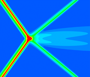
In the present work, the RR problem is considered in the following formulation. Two IS waves are generated by two wedges placed in a supersonic viscous flow. A typical flow structure is presented in figure 2. Dashed green lines on the plot denote upstream and downstream viscous shock ‘boundaries’. They can be defined quite arbitrarily, e.g. by one per cent difference in density from the RH upstream and downstream values, and are plotted only for illustration purposes.

Figure 2. Flow structure in the RR problem.
The flow Mach number is defined as
 \begin{equation} Ma_\infty = \frac{v_\infty}{\sqrt{\gamma RT_\infty}} = \frac{v_\infty}{\sqrt{5 RT_\infty/3}}, \end{equation}
where  $v_\infty$ and $T_\infty$ are the free stream velocity and temperature, respectively. The Mach number and the angle of the wedge, $\theta _w$, are specifically chosen to ensure that the RR is possible and the Mach reflection is impossible. The angle of both IS and RS, as well as the flow parameters behind them can be determined analytically. We consider the case where the flow remains supersonic downstream of the RR area. Computations are conducted for the free stream Mach number $Ma_\infty =20$ and the wedge angle $\theta _w = 17.061^\circ$. Under these conditions, the Mach number normal to the IS $Ma_n$ is equal to 8; therefore, the IS is equally strong to the considered 1-D planar shock so that one can expect a comparable degree of thermal non-equilibrium in the two problems under consideration. This fact allows for meaningful qualitative comparisons of the planar shock and RR results.
The Knudsen number for the considered flow can be defined as the ratio of the free stream mean free path  $\lambda _\infty$ to the length of the windward side of the wedge $w$:
$w$:
 \begin{equation} Kn = \frac{\lambda_\infty}{w}. \end{equation}
The free stream mean free path for the variable hard sphere (VHS) molecular model (see Bird Reference Bird1994) consistent with the power-law viscosity dependence on temperature is defined by
 \begin{equation} \lambda_{\infty} = \frac{2(5 - 2\omega)(7 - 2\omega)}{15\sqrt{\rm \pi}} \frac{\mu_{\infty}}{\rho_{\infty}\sqrt{2 RT_\infty}}, \end{equation}
where  $\rho _{\infty }$ and $\mu _{\infty }$ are free stream values of density and dynamic viscosity, respectively.
The Reynolds number for this flow can be defined as follows:
 \begin{equation} {\textit{Re}} = \frac {\rho_{\infty} v_\infty w } { \mu_{\infty} }. \end{equation}
For the VHS molecules it can be calculated from the Mach and Knudsen numbers with the following expression:
 \begin{equation} {\textit{Re}} = \frac{2 (5 - 2\omega) (7 - 2\omega) }{15 \sqrt{\rm \pi}} \sqrt{\frac{ \gamma }{2 }} \frac{Ma_\infty }{Kn}. \end{equation}
 In the present work the wedges are used only for generation of the shock waves; only a relatively small zone in the near vicinity of the reflection point is analysed which is independent of the macroscopic length scale  $w$. Apart from the molecular collision model parameters for considered monatomic gas with power-law viscosity dependence on temperature, such a problem has only two similarity parameters: Mach number $Ma_\infty$ and wedge angle $\theta _w$ (alternatively, $Ma_n$ can be used instead of $Ma_\infty$ or the angle between the IS and plane of symmetry, which equals 23.58 $^\circ$ in the present study, instead of $\theta _w$). The choice of the Knudsen number is therefore quite arbitrary: it only should be low enough for the shock wave thickness to be much smaller than the size of the computational domain. In particular, the zone of interest about the reflection point must be small enough so the expansion fans which emanate from the trailing edges of the wedges do not affect it. The Knudsen number of 0.001 is considered in the present study, which corresponds to the Reynolds number of 27 185. The distance between the trailing edges of the wedges, which is also an arbitrary parameter chosen using similar considerations, is 0.2132 $w$.
$w$.
Computations performed by all numerical techniques employ similar boundary conditions. Non-permeability boundary conditions (specular reflection of molecules in the DSMC method) are used for the wedge surface (the wedge is used only for IS generation; therefore, the boundary layer is ignored). The free stream parameters are imposed on the left boundary. Supersonic outflow is used on the right boundary (in the DSMC method, free outflow is considered with no molecules entering the computational domain).
3. Gas flow models and numerical methods
3.1. The Navier–Stokes–Fourier equations
The NSF equations for compressible flows can be obtained by the Chapman–Enskog expansion from the kinetic Boltzmann equation (Kogan Reference Kogan1969; Chapman & Cowling Reference Chapman and Cowling1991). The conservation laws of mass, momentum and energy correspondingly are as follows:
 $$\begin{gather} \frac{\partial \rho }{\partial t}+\frac{\partial \rho {{v }_{k}}}{\partial {{x}_{k}}}=0, \end{gather}$$
 $$\begin{gather}\rho \frac{\partial {{v }_{i}}}{\partial t}+\rho {{v }_{k}}\frac{\partial {{v }_{i}}}{\partial {{x}_{k}}}+\frac{\partial p}{\partial {{x}_{i}}}+\frac{\partial {{\mathsf{\sigma}}_{ik}^{NSF}}}{\partial {{x}_{k}}}=0, \end{gather}$$
 $$\begin{gather}\frac{3}{2}\rho \frac{\partial \theta }{\partial t}+\frac{3}{2}\rho {{v }_{k}}\frac{\partial \theta }{\partial {{x}_{k}}}+\frac{\partial {{q}_{k}^{NSF}}}{\partial {{x}_{k}}}+p\frac{\partial {{v }_{k}}}{\partial {{x}_{k}}}+{{\mathsf{\sigma}}_{ij}^{NSF}}\frac{\partial {{v }_{i}}}{\partial {{x}_{j}}}=0, \end{gather}$$
where the mass density  $\rho$, velocity $v_i$, temperature $\theta$ in energy units $\theta =({k}/{m})T=RT$ ( $k$ is the Boltzmann constant, $m$ is the molecular mass and $R=k/m$ is the gas constant), trace-free viscous stress tensor ${\mathsf{\sigma}}_{ij}$ (with ${\mathsf{\sigma}}_{kk}={\mathsf{\sigma}}_{11}+{\mathsf{\sigma}}_{22}+{\mathsf{\sigma}}_{33}$ = 0) and heat flux $q_i$ form 13 variables in three-dimensional case. The pressure is given by the ideal gas law $p=\rho \theta$. The Chapman–Enskog method yields the Navier–Stokes and Fourier laws for monatomic gas with the Prandtl number of 2/3 as
 \begin{equation} {\mathsf{\sigma}}_{ij}^{NSF} ={-}2\mu \frac{\partial{{v}_{\langle {i}}}}{\partial {{x}_{j\rangle}}},\quad q_{i}^{NSF} ={-}\frac{15}{4}\mu \frac{\partial \theta }{\partial {{x}_{i}}} \end{equation}
with the viscosity coefficient  $\mu$ calculated using a temperature–viscosity exponent of 0.72. The angular brackets in the subscripts indicate the trace-free and symmetric part of the tensor (Struchtrup Reference Struchtrup2005). The NSF equations are numerically solved with two independent flow solvers: CFS3D and ANSYS Fluent. The CFS3D solver is a time-explicit shock-capturing code developed at the Khristianovich Institute of Theoretical and Applied Mechanics and it is based on a fifth-order weighted essentially non-oscillatory reconstruction (Jiang & Shu Reference Jiang and Shu1996) of convective terms and a mixed, central-biased, fourth-order approximation of dissipation terms (Kudryavtsev & Khotyanovsky Reference Kudryavtsev and Khotyanovsky2005). Time marching is performed with the second-order Runge–Kutta scheme. Computations performed with ANSYS Fluent use a density-based solver in a steady formulation with the second-order upwind scheme for convective terms and the second-order central difference scheme for dissipation terms. The other details of the flow-solver set-up can be found in Shoev & Ogawa (Reference Shoev and Ogawa2019). Both NSF flow solvers showed identical numerical solutions, therefore we do not distinguish them further.
3.2. The regularized 13-moment equations
The regularization of Grad's original 13-moment system (Grad Reference Grad1949; Kogan Reference Kogan1969) was conducted in 2003 (Struchtrup & Torrilhon Reference Struchtrup and Torrilhon2003) by a Chapman–Enskog expansion (Chapman & Cowling Reference Chapman and Cowling1991) of higher moment equations only, based on the assumption of faster relaxation times for higher moments. Since relaxation times for moments only vary slightly between different moments, this assumption is somewhat artificial. So later derivations of the R13 equations were developed explicitly without this assumption (Struchtrup Reference Struchtrup2005). There are many examples of successful applications of this system of equations for slow moderately rarefied flows (Torrilhon & Struchtrup Reference Torrilhon and Struchtrup2008; Timokhin, Ivanov & Kryukov Reference Timokhin, Ivanov and Kryukov2014; Torrilhon Reference Torrilhon2016; Claydon et al. Reference Claydon, Shrestha, Rana, Sprittles and Lockerby2017; Baliti, Hssikou & Alaoui Reference Baliti, Hssikou and Alaoui2019; Westerkamp & Torrilhon Reference Westerkamp and Torrilhon2019). It has been shown that the R13 equations predict the internal structure of shock waves quite accurately (Torrilhon & Struchtrup Reference Torrilhon and Struchtrup2004; Timokhin et al. Reference Timokhin, Bondar, Kokhanchik, Ivanov, Ivanov and Kryukov2015, Reference Timokhin, Struchtrup, Kokhanchik and Bondar2017) and can be successfully applied to modelling of supersonic flows (Torrilhon Reference Torrilhon2006; Znamenskaya et al. Reference Znamenskaya, Ivanov, Kryukov, Mursenkova and Timokhin2014; Timokhin, Ivanov & Kryukov Reference Timokhin, Ivanov and Kryukov2018; Timokhin et al. Reference Timokhin, Struchtrup, Kokhanchik and Bondar2019). The tensor form of the regularized 13-moment system (R13) can be written as
 $$\begin{gather} \frac{\partial \rho }{\partial t}+\frac{\partial \rho {{v }_{k}}}{\partial {{x}_{k}}}=0, \end{gather}$$
 $$\begin{gather}\rho \frac{\partial {{v }_{i}}}{\partial t} + \rho {{v }_{k}}\frac{\partial {{v }_{i}}}{\partial {{x}_{k}}} + \frac{\partial p}{\partial {{x}_{i}}} + \frac{\partial {{\mathsf{\sigma}}_{ik}}}{\partial {{x}_{k}}}=0, \end{gather}$$
 $$\begin{gather}\frac{3}{2}\rho \frac{\partial \theta }{\partial t} + \frac{3}{2}\rho {{v }_{k}}\frac{\partial \theta }{\partial {{x}_{k}}} + \frac{\partial {{q}_{k}}}{\partial {{x}_{k}}} + p\frac{\partial {{v}_{k}}}{\partial {{x}_{k}}} + {{\mathsf{\sigma}}_{ij}}\frac{\partial {{v}_{i}}}{\partial {{x}_{j}}} = 0, \end{gather}$$
 $$\begin{gather}\frac{\partial {{\mathsf{\sigma}}_{ij}}}{\partial t} + \frac{\partial {{\mathsf{\sigma}}_{ij}}{{v }_{k}}}{\partial {{x}_{k}}} + \frac{4}{5}\frac{\partial {{q}_{\langle i}}}{\partial {{x}_{j\rangle }}} + 2p\frac{\partial {{v}_{\langle i}}}{\partial {{x}_{j\rangle }}} + 2{{\mathsf{\sigma}}_{k\langle i}}\frac{\partial {{v }_{j\rangle }}}{\partial {{x}_{k}}} + \frac{\partial {{\mathsf{m}}_{ijk}}}{\partial {{x}_{k}}}={-}\frac{{{\sigma }_{ij}}}{\tau}, \end{gather}$$
 \begin{align} & \frac{\partial {{q}_{i}}}{\partial t} + \frac{\partial {{q}_{i}}{{v }_{k}}}{\partial {{x}_{k}}}+\frac{5}{2}p\frac{\partial \theta }{\partial {{x}_{i}}} + \frac{5}{2}{{\mathsf{\sigma}}_{ik}}\frac{\partial \theta }{\partial {{x}_{k}}}+\theta \frac{\partial {{\mathsf{\sigma}}_{ik}}}{\partial {{x}_{k}}} \nonumber\\ &\quad -{{\mathsf{\sigma}}_{ik}}\theta \frac{\partial \rho }{\partial {{x}_{k}}} - \frac{{{\mathsf{\sigma}}_{ij}}}{\rho }\frac{\partial {{\mathsf{\sigma}}_{jk}}}{\partial {{x}_{k}}} + \frac{7}{5}{{q}_{k}}\frac{\partial {{v }_{i}}}{\partial {{x}_{k}}} + \frac{2}{5}{{q}_{k}}\frac{\partial {{v }_{k}}}{\partial {{x}_{i}}} \nonumber\\ &\quad + \frac{2}{5}{{q}_{i}}\frac{\partial{{v}_{k}}}{\partial {{x}_{k}}} + \frac{1}{2}\frac{\partial {{\mathsf{R}}_{ik}}}{\partial {{x}_{k}}} + \frac{1}{6}\frac{\partial \varDelta}{\partial {{x}_{i}}} + {{\mathsf{m}}_{ijk}}\frac{\partial {{v }_{j}}}{\partial {{x}_{k}}}={-} \frac{2}{3}\frac{{{q}_{i}}}{\tau }, \end{align}
where pressure is determined by the ideal gas law  $p=\rho \theta$ and $\tau ={\mu }/{p}$ is the relaxation time obtained with the viscosity coefficient $\mu$. Mass density $\rho$, velocity $v_i$, temperature in energy units $\theta$, trace-free viscous stress tensor ${\mathsf{\sigma}}_{ij}$ and heat flux $q_i$ form 13 primitive variables. Equations (3.5)–(3.7) are the conservation laws for mass, momentum and energy; (3.8) and (3.9) are the moment equations for the stress tensor and heat flux vector, respectively. These 13 equations must be closed by constitutive relations for the higher moments ${\mathsf{R}}_{ij}$, $\varDelta$, ${\mathsf{m}}_{ijk}$, and they differ based on the method of regularization. For Grad's original 13 moment equations (Grad Reference Grad1949), ${\mathsf{R}}_{ij} =\varDelta ={\mathsf{m}}_{ijk}=0$.
There are several nonlinear variants of the R13 equations which are different in higher-order moment relations (Struchtrup & Torrilhon Reference Struchtrup and Torrilhon2003; Struchtrup Reference Struchtrup2005; Rana & Struchtrup Reference Rana and Struchtrup2016; Timokhin et al. Reference Timokhin, Struchtrup, Kokhanchik and Bondar2016, Reference Timokhin, Struchtrup, Kokhanchik and Bondar2017). The linear variant of the R13 equations has been used in the present study. In the linear case (gradient transport mechanism (Gu & Emerson Reference Gu and Emerson2009)), higher-order moments have the following form:
 \begin{equation}
{{\mathsf{m}}_{ijk}}={-}2\tau
\theta\frac{\partial {{\mathsf{\sigma}}_{\langle ij}}}{\partial
{{x}_{k\rangle }}},\quad {{\mathsf{R}}_{ij}}={-}\frac{24}{5}\tau
\theta\frac{\partial {{q}_{\langle i}}}{\partial
{{x}_{j\rangle }}}, \quad \varDelta ={-}12\tau
\theta\frac{\partial {{q}_{l}}}{\partial {{x}_{l}}}.
\end{equation}
\begin{equation}
{{\mathsf{m}}_{ijk}}={-}2\tau
\theta\frac{\partial {{\mathsf{\sigma}}_{\langle ij}}}{\partial
{{x}_{k\rangle }}},\quad {{\mathsf{R}}_{ij}}={-}\frac{24}{5}\tau
\theta\frac{\partial {{q}_{\langle i}}}{\partial
{{x}_{j\rangle }}}, \quad \varDelta ={-}12\tau
\theta\frac{\partial {{q}_{l}}}{\partial {{x}_{l}}}.
\end{equation}The numerical method used for solving the R13 system in this work was described in detail by Ivanov, Kryukov & Timokhin (Reference Ivanov, Kryukov and Timokhin2013) and Timokhin et al. (Reference Timokhin, Bondar, Kokhanchik, Ivanov, Ivanov and Kryukov2015).
3.3. The DSMC method
The DSMC method is a numerical technique which treats the gas flow as an ensemble of model particles. Each model particle represents a large number ( ${\sim }10^{12}\unicode{x2013}10^{20}$) of real molecules (or atoms) of the gas. The modelling process is split into two independent stages at each time step $\Delta t$: free-molecular transfer and collisional relaxation. At the first stage the model particles are shifted by distances proportional to their velocities. If the model particle collides with the body surface during its free-molecular travel, its reflection is modelled in accordance with a specified law of gas–surface interaction. At the second stage, molecular collisions are simulated stochastically in each collisional cell of the computational domain, disregarding the mutual positions of the model particles. The spatial distributions of gas-dynamic parameters, such as velocity, density, temperature, etc., are obtained by averaging molecular properties sampled in each cell over some time interval after reaching the steady state.
The DSMC method can be considered a Monte Carlo method for the numerical solution of the kinetic Boltzmann equation when the number of model particles tends to infinity (see Ivanov & Rogasinsky Reference Ivanov and Rogasinsky1988). The DSMC solutions for the strong shock fronts are known to be in perfect agreement with the direct numerical solution of the Boltzmann equation (see e.g. Malkov et al. Reference Malkov, Bondar, Kokhanchik, Poleshkin and Ivanov2015). In the present work the DSMC results are considered benchmark solutions. The applicability and accuracy of the other two approaches are analysed by comparison with the DSMC method.
The DSMC computations are performed with the SMILE++ software system (Kashkovsky et al. Reference Kashkovsky, Bondar, Zhukova, Ivanov and Gimelshein2005; Ivanov et al. Reference Ivanov, Kashkovsky, Vashchenkov and Bondar2011) that is based on the majorant frequency scheme (Ivanov & Rogasinsky Reference Ivanov and Rogasinsky1988). The VHS model was applied for elastic collisions. The model is consistent with the power-law temperature dependence of viscosity used in both continuum methods and  $\omega$ can be considered its input parameter. At the start of the simulation process, the domain is populated by model particles according to the Maxwell distribution function corresponding to the free stream parameters. Then the computation is run until the steady state is reached and sampling of molecular properties begins in order to obtain macroparameter flow fields.
3.4. Accuracy of computational results
The grid for all three methods considered was fine enough providing the linear cell sizes are small in comparison with the local mean free path at the steady state. This means in all computations shock structures were well-resolved with dozens of grid points inside shock fronts. The computation time step in all methods was chosen small enough (smaller than mean collision time) to ensure high accuracy of results. All numerical data presented below can be considered grid- and timestep-independent. In the DSMC computations, the number of particles exceeded by orders of magnitudes all accuracy requirements (see e.g. Shevyrin, Bondar & Ivanov Reference Shevyrin, Bondar and Ivanov2005), and the sample size was large enough to make the statistical error negligible. A detailed analysis of the grid convergence of all three methods for the RR problem is presented in the Appendix.
4. Results and discussion
The following non-dimensionalization of the flow parameters is used in this section:
 \begin{equation} \left.\begin{gathered} {\widehat{v_i}}=\frac{v_i}{C_\infty},\quad {\hat{x}}=\frac{x}{\lambda_{\infty}},\quad {\hat{T}}={\hat{\theta}}=\frac{T}{T_\infty},\quad {\hat{\rho}}=\frac{\rho}{\rho_\infty}, \\ {\hat{p}}=\frac{p}{{\rho_\infty}{C_\infty^2}} = \frac{1}{2}\hat{\rho}\hat{T},\quad {\widehat{q_i}}=\frac{q_i}{{\rho_\infty}{C_\infty^3}},\quad {\hat{\mathsf{\sigma}}_{ij}}=\frac{\sigma_{ij}}{{\rho_\infty}{C_\infty^2}}, \end{gathered}\right\} \end{equation}
where  $C_\infty =\sqrt {2RT_\infty }$ is the absolute value of the free stream most probable peculiar molecular velocity. The $\infty$ subscript denotes the free stream values. Only non-dimensional variables (4.1) are used below in the present section with the ‘hat’ symbol omitted except for the non-dimensional coordinates in figures where they are denoted as $x / \lambda _{\infty }$ and $y / \lambda _{\infty }$.
4.1. General features of flow fields
The main focus of the present study is the relatively small region of the incident oblique shock wave reflection from the plane of symmetry. Figure 3 presents the numerical results of the distributions of dimensionless temperature in this region (see (4.1)) obtained by the NSF, R13 equations and DSMC. The point with the coordinates  $(0,0)$ is the reflection point obtained analytically from the inviscid solution (see figure 2). The black lines present the shock-wave discontinuities in the inviscid solution.

Figure 3. Temperature distribution fields for NSF (a), R13 (b) and DSMC (c).
All three considered viscous flow models predict non-uniform temperature behind the RS that shows essentially viscous and non-continuum effects since the inviscid continuum solution given by the Euler equations predicts the uniform flow behind the RS. In particular, they all predict the appearance of a 2-D maximum (overshoot) to the right of the point  $(0,0)$. The zone with the temperature maximum behind the RS is called the non-RH zone (Sternberg Reference Sternberg1959; Ivanov et al. Reference Ivanov, Bondar, Khotyanovsky, Kudryavtsev and Shoev2010; Shoev et al. Reference Shoev, Kudryavtsev, Khotyanovsky and Bondar2023) (this term was originally coined for the flow near the triple point in the irregular shock reflection). Indeed, the temperature value behind two oblique shocks given by RH conditions correspond to the orange colour in the legend. It is quite clear that all three approaches predict values of temperature that exceed the RH values.
The presence of a temperature extremum for the DSMC and R13 solutions might be expected in connection with similar results in the problem of the 1-D structure of the shock wave (see the § 4.2). The presence of an overshoot in the planar shock wave structure problem at large Mach numbers has been shown in many papers using both kinetic description (Elliott & Baganoff Reference Elliott and Baganoff1974; Erofeev & Friedlander Reference Erofeev and Friedlander2002; Dodulad & Tcheremissine Reference Dodulad and Tcheremissine2013; Malkov et al. Reference Malkov, Bondar, Kokhanchik, Poleshkin and Ivanov2015) and extended gas dynamics methods (Jin, Pareschi & Slemrod Reference Jin, Pareschi and Slemrod2002; Torrilhon & Struchtrup Reference Torrilhon and Struchtrup2004; Erofeev & Friedlander Reference Erofeev and Friedlander2007; Ivanov et al. Reference Ivanov, Kryukov, Timokhin, Bondar, Kokhanchik and Ivanov2012; Timokhin et al. Reference Timokhin, Bondar, Kokhanchik, Ivanov, Ivanov and Kryukov2015). In addition, it was shown that this maximum is observed at all types of molecular interaction potentials with the Mach number  $Ma \geq 3.9$ (Yen Reference Yen1984; Erofeev & Friedlander Reference Erofeev and Friedlander2002). At the same time, it can be shown (Struchtrup Reference Struchtrup2005) that it is impossible to obtain a non-monotonic temperature distribution in a planar shock wave with the NSF equations. It is interesting to obtain a temperature maximum in the NSF solution of this 2-D problem. The same effect was also demonstrated with the NSF equations by Khotyanovsky et al. (Reference Khotyanovsky, Bondar, Kudryavtsev, Shoev and Ivanov2009). These results suggest that the appearance of such a maximum is not due to non-equilibrium effects as in the planar shock wave case, but rather can be explained by 2-D effects (see § 4.4). Another difference between these two cases is that the planar shock overshoot is located within the shock front while the present 2-D results clearly indicate that the maximum is separated from the RS front (see figure 3). For the sake of clarity, in what follows the term ‘temperature overshoot’ is used for the planar shock wave maximum (which is also observed in oblique shock waves) and the term ‘temperature maximum’ is applied to the maximum which is observed on the symmetry plane in the RR problem.
As it can be seen from the comparison of temperature flow fields in figure 3, the numerical results by the R13 equations turn out to be not only qualitatively but quantitatively very close to the DSMC kinetic solution. Figure 4 presents a comparison of temperature isolines for all three numerical approaches (figure 4a gives NSF versus R13, and figure 4b gives DSMC versus R13). The NSF numerical solution is far from the R13 numerical solution – R13 demonstrates greater thickness for both IS and RS waves. This disagreement is expected since the NSF equations fail to predict the internal structure of a shock wave accurately if the Mach number of the free stream is higher than  $Ma=2.0$ (Pham-Van-Diep, Erwin & Muntz Reference Pham-Van-Diep, Erwin and Muntz1991). The R13 results agree with the DSMC benchmark solution quite well. The quantitative agreement between the two methods improves with the decreasing of the local Mach number (as it moves downstream). This R13 equations’ behaviour is similar to that in the 1-D shock wave structure problem, where the fast upstream part of a shock wave is predicted much more poorly than the downstream slower flow part (Timokhin et al. Reference Timokhin, Struchtrup, Kokhanchik and Bondar2017).

Figure 4. Temperature isolines for NSF–R13 (a) and R13–DSMC (b).
Figure 5 presents the comparison of the density and temperature profiles for all three models over horizontal cross-sections at different distances from the symmetry plane. The curves at finite distances from the symmetry plane consist of distinct incident oblique and RS-wave profiles and areas of nearly uniform flow (zones (1), (2), (3) in figure 1) while the curves for the  $y=0$ cross-section resemble ordinary planar 1-D shock-wave profiles (IS and RS fronts are merged into one). The profiles along the symmetry plane for all three models also clearly reveal a temperature maximum which was observed in the flow fields. The maximum exceeds 5 per cent for the DSMC and R13 and is much smaller for the NS. The density profile along the symmetry plane especially for the R13 and DSMC case lies below the RH value of density behind IS and RS even a hundred mean free paths downstream of the reflection point. It is consistent with the long wake observed in the temperature flow fields. It is interesting that at the distance of five and 10 mean free paths from the symmetry plane all the density profiles reach the RH value rapidly as in a typical shock wave, although tiny overshoots are observed in the DSMC and R13 density profiles.

Figure 5. Profiles of density (a) and temperature (b) for NSF, R13 and DSMC along  $x$ at $y=0.0$, $y=5\lambda _\infty$, $y=10\lambda _\infty$ and $y=15\lambda _\infty$. Dashed lines show RH values behind incident (bottom) and reflected (top) shocks.
The NSF equations provide results that are significantly different from the benchmark DSMC solution. As can be expected, disagreement is observed inside both IS and RS: the NSF model significantly underpredicts thickness of the shock front and does not predict a temperature overshoot inside the IS at various distances from the symmetry plane (a purely 1-D effect predicted by the R13 and DSMC for high Mach numbers). This 1-D overshoot is shown in the zoomed zone of the figure 5(b). The other difference is that the effects mentioned above (the temperature maximum on the symmetry plane and long downstream density tail lying below the RH value) are not prominent in the NSF solution. On the contrary, the distributions of the macroparameters of the R13 moment solution are quantitatively consistent with the DSMC kinetic solution in all cross-sections. The exceptions include the overestimated 1-D temperature overshoot in the IS and temperature distributions in the region of formation of the leading front of shock waves. Both of these effects are well known (see the results of Timokhin et al. (Reference Timokhin, Bondar, Kokhanchik, Ivanov, Ivanov and Kryukov2015) and Timokhin et al. (Reference Timokhin, Struchtrup, Kokhanchik and Bondar2017)). Another small difference is slight overestimation of the temperature maximum on the symmetry plane by the R13 equations.
Figure 6 presents the results for temperature and density in the cross-sections perpendicular to the flow direction in the free stream: along  $x=-20.6\lambda _\infty$, $x=0$ and $x=20.6\lambda _\infty$ lines. Two velocity components in the same cross-sections are shown in figure 7. Solid black lines present the inviscid solution on both sides of the shock waves. The dashed vertical lines show the positions of the IS and RS. The R13 results inside the fronts of oblique shock waves (parts of the profiles for $x = -20.6\lambda _\infty$ and $x =20.6\lambda _\infty$) turn out to be much closer to the reference DSMC solution than the NSF equations solution. The qualitative behaviour of the solutions by all three approaches is similar for the main flow macroparameters.

Figure 6. Profiles of density and temperature for NSF, R13 and DSMC along  $y$ at $x=-20.6\lambda _\infty$, $x=0$ and $x=20.6\lambda _\infty$.

Figure 7. Profiles of velocity components for NSF, R13 and DSMC along  $y$ at $x=-20.6\lambda _\infty$, $x=0$ and $x=20.6\lambda _\infty$.
Note, that the inviscid solution for temperature, density and flow velocity is constant for  $x=0$ and equal to their values behind the IS. For all three models of the viscous flow one observes clearly non-constant solutions in this cross-section. In particular, temperature exhibits more than a 50 per cent maximum in comparison with its value behind the IS. The NSF equations underpredict the temperature in this zone while the R13 equations overpredict the maximum value of the temperature in the vicinity of the origin. There are also visible non-uniformities in the R13 and NS density profiles and an $x$-velocity minimum in the origin. The value of this minimum is overpredicted by the R13 model while the NSF model predicts it accurately.
The quantitative difference between the three models under consideration for all the variables become smaller with increasing  $x$-coordinate. Most significant differences are observed for the upstream cross-section ( $x=-20.6\lambda _\infty$), while the downstream cross-section ( $x=20.6\lambda _\infty$) reveals the smallest difference between all three models. In this case, the results of the R13 equations almost repeat the DSMC data profiles. This trend correlates with the decrease in the local Mach number and increase of density of the flow downstream. It is interesting to notice that in the downstream cross-section near the symmetry plane the DSMC and R13 models predict temperature higher and $x$-velocity lower than that given by the RH conditions. It agrees with the figures shown above which confirm the existence of the large non-RH-zone behind the point of the shock-wave reflection.
4.2. Comparison of structures of the planar shock wave and the zone of the RR of an oblique shock wave
The flow fields and profiles of macroparameters along the symmetry plane presented in the previous subsection demonstrates that the area in the vicinity of the reflection point where IS and RS merge resembles an ordinary normal shock (such as Mach stem in the case of Mach reflection, see e.g. Ben-Dor Reference Ben-Dor2007) with macroparameter isolines normal to the symmetry plane and a steep rise of density and temperature along the streamline. The present section is devoted to the analysis of the similarities and differences in the macroparameters’ distributions of the NSF, R13 and DSMC solutions in the 1-D normal shock and along the symmetry plane in the 2-D RR flow. Recall, that we consider the normal shock wave with Mach number  $Ma= 8.0$ equal to the normal Mach number for the IS in the RR case, $Ma_n=8.0$ to ensure comparable degree of thermal non-equilibrium inside the shocks in both flows. Below, macroparameters’ comparison is presented starting with zeroth- and first-order moments of the distribution function (density and velocity) and moving on to higher-order moments such as temperature, viscous stress tensor and heat flux. The origin for the normal shock wave case is located in the shock centre – a point with the density equal to the mean value of the densities upstream and downstream of the shock.
The figures 8, 9 and 10 present density, velocity and temperature profiles for both flows obtained with all three gas flow models. The black lines here illustrate the inviscid solutions. As it can be seen from the profiles, the thickness of the 1-D shock wave (characterized by maximal slope of the profile) is approximately 10 mean free paths, while the thickness of the 2-D structure along the symmetry plane in the RR case is more than two times greater. The reference DSMC solution in the 2-D RR case reveals that a very long tail is observed after the steep part of the profile with all the macroparameters reaching the RH values rather slowly in comparison with the normal shock case. While it takes approximately five mean free paths from the origin to reach the RH values in the normal shock case, in the 2-D RR case density, velocity and temperature are substantially different from the RH values 35 mean free paths downstream of the origin, or in other words the non-RH-zone is observed. The velocity profiles for the two cases considered have a qualitative difference in the region behind the shock wave front. A minimum of velocity is observed in the problem of RR in the non-RH-zone (figure 9b). Its position coincides with the position of the temperature maximum (figure 10b).

Figure 8. The NSF, R13 and DSMC density profiles for the 1-D shock structure problem (a) and 2-D RR problem (b).

Figure 9. The NSF, R13 and DSMC velocity profiles for the 1-D shock structure problem (a) and 2-D RR problem (b).

Figure 10. The NSF, R13 and DSMC temperature profiles for the 1-D shock structure problem (a) and 2-D RR problem (b).
The NSF equations greatly underestimate the thickness of the shock structures in both cases (the slope of the profiles is almost two times steeper than for the DSMC solution). The R13 solution agrees well with the DSMC one for density. A significant difference is observed in velocity and temperature at the leading edge of the shock wave which is manifested in a longer upstream tail of the DSMC profile (figures 9a and 10a). A detailed discussion of the behaviour of shock-wave solutions of various variants of the R13 system is given by Timokhin et al. (Reference Timokhin, Struchtrup, Kokhanchik and Bondar2017).
As it was mentioned above, both the R13 equations and the DSMC method predict temperature overshoot in the planar shock wave (see figure 10a) while the NSF solution is monotonic. For  $Ma_\infty =8$ the size of the overshoot in the DSMC solution is approximately $1\,\%$ with respect to the value behind the shock front. The overshoot in the R13 solution is much bigger (approximately $3\,\%$), and the NSF temperature profile does not have this peak at all. For the flow along the plane of symmetry (see figure 10b), all models considered predict a temperature maximum, and its value in the DSMC and R13 solutions is approximately 5 % with respect to the downstream temperature, which is substantially greater than the maximum predicted by the NSF solution (approximately 2 %).
The distribution of temperatures associated with thermal motion of molecules in different directions can provide additional information on the structure of the flows under consideration. Gas temperature can be represented as follows:
 \begin{equation} T= \tfrac{1}{3} (T_x + T_y + T_z), \end{equation}
where  $T_x$, $T_y$ and $T_z$ are kinetic temperatures defined by mean energy of thermal motion of molecules in the $x$,
$x$,  $y$ and $z$ directions (temperature components or $x$-,
$x$-,  $y$- and $z$-temperature, respectively). The following expressions relate these temperatures to the diagonal components of stress tensor in the non-dimensional form (4.1):
 $$\begin{gather} \theta_x=T_x=2(p+\sigma_{xx})/\rho, \end{gather}$$
 $$\begin{gather}\theta_y=T_y=2(p+\sigma_{yy})/\rho, \end{gather}$$
 $$\begin{gather}\theta_z=T_z=2(p+\sigma_{zz})/\rho. \end{gather}$$
In the problem of the structure of a planar shock wave, so called transverse temperatures  $T_y$ and $T_z$ are equal to each other. So an overall gas temperature (4.2) in the 1-D case can be written as $T= \frac {1}{3} ( T_x + 2T_y )$.
Figures 11 and 12 show the comparisons of the temperature components for both problems obtained using all three approaches. In figure 11 NSF and DSMC results are presented. As for other macroparameters the NSF solution predicts much steeper slope and much less gradual onset of the profiles for both problems. Except for these differences the NSF and DSMC profiles are qualitatively similar for the planar shock wave case: streamwise temperature  $T_x$ has a significant maximum while transverse temperature $T_y$ increases monotonically and the RH postshock value is reached within five free stream mean free paths by both temperatures. Moreover, the value of the streamwise temperature maximum in the planar shock wave is similar for both gas flow models, which is predicted by Yen's solution (Yen Reference Yen1966). The profiles of temperature components for the 2-D RR profile reveal the similar differences between the NSF and DSMC results from the planar shock wave cases witnessed above: the zone of steep gradients is approximately two times thicker and a very long non-RH-zone is observed downstream.

Figure 11. Different components of temperature predicted by the NSF and DSMC. The 1-D shock-wave structure (a) and internal structure of RR along the symmetry plane (b).

Figure 12. Different components of temperature predicted by the R13 and DSMC. The 1-D shock-wave structure (a) and internal structure of RR along the symmetry plane (b).
All temperature distributions provided by the R13 are much closer to the DSMC data for both problems (see figure 12) as it can be expected from the profiles of the macroparameters analysed above. However, longer upstream tails in the DSMC distributions are observed similar to other macroparameters. Note, that in the RR  $x$ and $y$ temperature components are overpredicted by the R13 near the origin. These overestimated values of these two temperature components lead to an overestimated value of the total temperature in this region (see figure 5b for $y=0$).
The most significant qualitative difference in distributions of directional temperatures between the two problems under consideration, is that in the RR the mentioned streamwise temperature maximum is not observed at all. Instead all three approaches predict prominent maxima of  $T_y$ temperature near the origin, while $T_x$ and $T_z$ temperature are very close to each other and steadily increase up to the point of equalization of all three directional temperatures. Farther downstream all the temperatures decrease down to the RH value, so, strictly speaking, all three temperatures exhibit a non-monotonic behaviour. This $T_y$ maximum can be explained by a sharp flow deceleration along the $y$-direction to a zero value of velocity $y$-component on the plane of symmetry in the vicinity of the point of origin (0,0). This part of the kinetic energy goes into thermal molecular motion. Obviously, the translational $y$-temperature must get more energy. At the same time, the molecules need time to undergo a sufficient number of collisions to dissipate thermal motion over all translational molecular degrees of freedom. This local thermal non-equilibrium leads to such behaviour of directional temperatures observed in figures 11(b) and 12(b).
Figures 13 and 14 present a comparison of the components of the viscous stress tensor and the longitudinal heat flux component in the same format as above. The heat flux is the highest moment of the local distribution function among considered. Therefore, one can expect a greater difference in the results of continuum approaches from the kinetic solution. Figures 13(a) and 14(a) compare the results of the NSF, R13 and DSMC for the normal shock. As it can be seen, the results of the R13 equations are in good agreement with the low-speed part of the DSMC shock wave front. The extrema for both macroparameters are predicted fairly accurately by the R13 equations. At the same time, significant differences are observed in the high-speed part of the structure. The NSF equations provide  ${\mathsf{\sigma}} _{xx}$ and $q_x$ distributions which is significantly different from the DSMC ones: the value of the viscous stress maximum is overpredicted by 20 % while the value of the heat flux minimum is underpredicted by the same degree.

Figure 13. The  $\sigma$-components predicted by NSF, R13 and DSMC. The 1-D shock-wave structure (a) and internal structure of RR along the symmetry plane (b).

Figure 14. The  $q_{x}$ predicted by NSF, R13 and DSMC. The 1-D shock-wave structure (a) and internal structure of RR along the symmetry plane (b).
Due to the presence of a large transverse gradient of the  $y$-velocity component (see § 4.4) near the RR point, the behaviour of the components of the viscous stress tensor differs qualitatively from the results of the 1-D problem. Figure 13(b) shows the distributions of the components ${\mathsf{\sigma}} _{xx}$ and ${\mathsf{\sigma}} _{yy}$ obtained by all the proposed methods. Figure 14(b) presents a similar comparison of the longitudinal heat flux $q_x$. As it can be seen from the both figures, the difference between the R13 and the DSMC solution appears to be significant in the entire considered region. The absolute values of the extrema are underestimated by the R13 equations (the differences reach approximately 20 %). Moreover, the NSF equations overestimate the absolute values of extrema by up to 30 %. The qualitative behaviour of the viscous stress tensor diagonal components is in agreement with the distributions of directional temperatures (see figures 11 and 12) which are related to them by (4.3)–(4.5).
4.3. The 2-D effects in the confluence of the incident and reflected shock wave
The present subsection aims at explaining the effects in the flow along the symmetry plane streamline in the RR discussed in the previous subsection. Let us first start with the flow at some distance from the symmetry plane where the IS and RS fronts can be separated from one another.
As mentioned above, the considered free stream Mach number  $Ma=20$ and the wedge angle $\theta _w=17.061$ correspond to the normal Mach number $Ma_n=8$ of the incident oblique shock wave. The normal Mach number for the oblique RS wave in the considered case is $Ma_n=2.1$. It is well known that the RH conditions across any oblique shock are similar to the normal shock if one formulates them in terms of the normal Mach number and takes into account that the tangential flow velocity component is equal on both sides of the shock front (see e.g. Landau & Lifshitz Reference Landau and Lifshitz1987). Moreover, the problem of internal structure of an oblique shock wave can be reduced to a problem of internal structure of a normal shock by considering it in the frame of reference which is moving with the component of the free stream velocity tangential to the shock front. In this frame of reference tangential gas velocity becomes equal to zero and the problem formulation fully coincides with that of the 1-D normal shock. Hence the structures of the normal and oblique shocks differ only in the presence of the constant tangential component of flow velocity in the latter case.
The profiles across the IS and RS along the free stream direction ( $x$ axis, symmetry plane) at different $y$-coordinate were compared with the planar shock wave profiles computed at $Ma=8.0$ and $Ma=2.1$. For the sake of such comparison the normal shock profiles were linearly transformed from the shock-front reference frame to the laboratory reference frame. The scheme of such a transformation is shown in figure 15. A planar shock wave lies schematically between two blue lines. The red segment AB is the shock wave profile along the normal to the shock front, and the green segment AC is the result of the transformation (non-orthogonal projection in the direction parallel to the shock front onto the $x$ axis). In order to obtain the required shock wave profile along the AC segment the coordinate across the original 1-D normal shock profile (AB segment) is divided by the sine of the oblique shock angle.

Figure 15. Scheme of comparison between 1-D and 2-D numerical results.
The comparison series of the NSF results of transformed temperature distributions for two 1-D shock waves and the results for the 2-D RR problem is presented in figure 16 in decreasing order of distance to the symmetry plane (for  $y=\{15\lambda _\infty$, $8\lambda _\infty$, $3\lambda _\infty$ and $0\lambda _\infty \}$). The red and green curves represent the projections of the 1-D profiles of the IS and RS, respectively. Symbols indicate the results of the regular reflection computation. Far from the reflection point, the results of two 1-D shock waves exactly repeat the 2-D solution (see the first two plots in figure 16 for $y = 15\lambda _\infty$ and $y=8\lambda _\infty$). This indicates the absence of 2-D effects of the investigated flow at such a distance. As one approaches the symmetry plane, at a distance of the order of a mean free path, 2-D effects start playing a significant role in the distribution of macroparameters in the vicinity of the reflection point: two shock waves merge in the RR problem (see the other two plots in figure 16 for $y = 3\lambda _\infty$ and $y = 0\lambda _\infty$). In addition to the difference in the region around the point $x = 0$, the temperature maximum is observed in the 2-D problem when it cannot be predicted by 1-D computations.

Figure 16. Comparison between transformed 1-D temperature distributions and temperature distributions in the RR problem at  $y=$ const. (NSF).
Similar results obtained with the DSMC method are presented in figure 17. At a distance of 15 mean free paths from the symmetry plane the IS and RS do not affect each other (2-D effects are negligible) and the RR profile coincides with the 1-D solutions as in the NSF case. At a distance of eight mean free paths, however, some minor 2-D effects are seen in the profile of the RS: temperature immediately behind the shock is slightly smaller than in the 1-D case and approaches the RH value farther downstream. This result is consistent with temperature isolines presented in figure 4. In the other two plots for  $y = 3\lambda _\infty$ and $y = 0\lambda _\infty$ one can observe clear 2-D merging of two shocks with a much more prominent temperature maximum in the DSMC solution than in the NSF one. The R13 model provides qualitatively similar results to the DSMC (not presented in the plots).

Figure 17. Comparison between transformed 1-D temperature distributions and temperature distributions in the RR problem at  $y=$ const. (DSMC).
Profiles of directional temperatures  $T_x$, $T_y$ and $T_z$ for various distances from the symmetry plane are presented in figures 18 and 19 for all three gas flow models. Despite the clearly demonstrated fact that internal structure of an oblique shock coincides with that of a normal shock, these profiles exhibit unexpected pronounced overshoots of $T_y$ inside the fronts while $T_x$ and $T_z$ are monotonic. Recall, that an overshoot of $T_x$ is typical for a normal shock. This seeming contradiction is explained by the choice of the axis direction in these two problems. Indeed, the $T_x$ temperature in the RR problem is not associated with thermal motion of molecules in the direction normal to the front but rather in the direction of the free stream. Due to significant inclination of both IS and RS with respect to the free stream (more than 45 degrees) the thermal motion of the molecules in the direction normal to the shocks mainly contribute to the $T_y$ temperature which explains its overshoots inside the shock fronts. With decreasing distance from the symmetry plane, $T_y$ overshoots start to merge and eventually form the sole overshoot at the symmetry plane for all three gas flow models under consideration. This fact clearly explains the presence of the $T_y$ overshoot discussed in the previous subsection as a result of the confluence of two shocks each of which has its own $T_y$ overshoot.

Figure 18. Temperatures  $T_x$, $T_y$ and $T_z$ at $y=$ const. for the RR problem. The NSF and DSMC results: $y=10\lambda _\infty$ (a), $y=5\lambda _\infty$ (b), $y=3\lambda _\infty$ (c), $y=0\lambda _\infty$ (d).

Figure 19. Temperatures  $T_x$, $T_y$ and $T_z$ at $y=$ const. for the RR problem. The R13 and DSMC results: $y=10\lambda _\infty$ (a), $y=5\lambda _\infty$ (b), $y=3\lambda _\infty$ (c), $y=0\lambda _\infty$ (d).
4.4. Analyses of the flow with conservation equations
The results on RR presented above clearly demonstrate deviation from the RH values downstream of the reflection point, e.g. the existence of a non-RH zone. Recall, that the RH relations can be considered as a corollary of the 1-D conservation laws. Deviation from the RH relations can be explained by 2-D effects in the region of the shock reflections. In order to clarify which processes are important in this regard an analysis of mass, momentum and energy conservation equations is performed for the symmetry plane streamline. In addition, the normal shock problem is also considered. Note, that the conservation equations are presented in the general form. All of them directly follow from the Boltzmann equation and must hold for any dilute gas flow model, including the three models employed in the present paper. As the R13 equations provide results which are qualitatively consistent with the DSMC ones, only the NSF and R13 models were used in the analyses.
The mass and momentum conservation equations for a steady 2-D flow along the plane of symmetry streamline can be written in terms of the substantial derivatives
 \begin{equation} \frac{{\rm D}}{{\rm D} t} = \frac{\partial}{\partial t} + v_x \frac{\partial}{\partial x} +\underline{v_y \frac{\partial}{\partial y}} = v_x \frac{\partial}{\partial x} +\underline{v_y \frac{\partial}{\partial y}} \end{equation}
as follows:
 $$\begin{gather} \frac{{\rm D} \rho}{{\rm D} t} ={-} \rho \left(\frac{\partial v_x}{\partial x} + \underline{\frac{\partial v_y}{\partial y}}\right), \end{gather}$$
 $$\begin{gather}\frac{{\rm D} v_x }{{\rm D} t} ={-} \frac{1}{\rho} \left(\frac{\partial p}{\partial x} + \frac{\partial {\mathsf{\sigma}}_{xx}}{\partial x} + \underline{\frac{\partial {\mathsf{\sigma}}_{xy}}{\partial y}}\right). \end{gather}$$
The underlined terms are caused by the two-dimensionality of the flow. The rest of the terms remain in the 1-D case of a planar shock wave structure problem.
The energy conservation law along the symmetry plane has the following form:
 \begin{equation} \frac{{\rm D} E }{{\rm D} t} ={-} \frac{1}{\rho} \left(\frac{\partial v_xp}{\partial x} + \frac{\partial v_yp}{\partial y}+ \frac{\partial v_x{\mathsf{\sigma}}_{xx}} {\partial x} + \frac{\partial v_x{\mathsf{\sigma}}_{xy}}{\partial y}+ \frac{\partial v_y{\mathsf{\sigma}}_{yy}}{\partial y} + \frac{\partial q_x}{\partial x}+ \frac{\partial q_y}{\partial y} \right), \end{equation}
where  $E$ is the total internal energy per unit mass containing kinetic $E_K = {v^2}/{2}$ and internal $E_I = e$ parts,
 \begin{equation} E = E_K + E_I = \frac{v^2}{2} + e = \frac{v^2}{2} + \frac{3}{4} T. \end{equation}
This form of the conservation laws allows one to analyse an evolution of density, velocity and total internal energy of a ‘fluid element’ of a constant mass and variable volume as it moves along the streamline (see e.g. Anderson Reference Anderson2019). The rates of change of these three parameters are determined by the terms on the right-hand side of the equations, which describe various physical processes, to be discussed below in detail. The term ‘fluid element’ typical of conventional continuum fluid dynamics is used hereafter for convenience. Note, that it should not be understood literally because all three considered gas flow models presume exchange of molecules between such an imaginary element and the gas medium which surrounds it.
To illustrate the influence and physical meaning of the right-hand part terms of the energy conservation equation (4.9) let us rewrite it taking into account that the terms  $v_y({\partial p}/{\partial y})$, $v_y ({\partial {\mathsf{\sigma}} _{yy}}/{\partial y})$ and ${\mathsf{\sigma}} _{xy} ({\partial v_x}/{\partial y})$ are equal to zero on the symmetry plane
 \begin{align} \frac{{\rm D} E }{{\rm D} t} &={-} \frac{1}{\rho} \left( v_x \frac{\partial p} {\partial x} + p \frac{\partial v_x} {\partial x}+ v_x \frac{\partial {\mathsf{\sigma}}_{xx}} {\partial x} + {\mathsf{\sigma}}_{xx} \frac{\partial v_x} {\partial x} + \frac{\partial q_x} {\partial x} \right. \nonumber\\ &\quad \left.+ \underline{v_x \frac{\partial {\mathsf{\sigma}}_{xy}} {\partial y} } + \underline{p \frac{\partial v_y} {\partial y} } + \underline{{\mathsf{\sigma}}_{yy} \frac{\partial v_y} {\partial y} } + \underline{\frac{\partial q_y} {\partial y} }\right), \end{align}
where the underlined terms are present only in the 2-D RR problem and hence describe 2-D effects on the symmetry plane. Equation (4.11) can be rewritten into two governing equations for kinetic and internal parts of  $E$ (see e.g. Anderson Reference Anderson2019) as follows:
 $$\begin{gather} \frac{{\rm D}}{{\rm D}
t} \left( \frac{v^2}{2} \right) = \underbrace{-
\frac{1}{\rho} \left( v_x \frac{\partial p} {\partial x} +
v_x \frac{\partial {\mathsf{\sigma}}_{xx}} {\partial x}
\right)}_{{P_{xx}\ gradient\ power}\quad}
\underbrace{-\underline{\frac{1}{\rho}\left(v_x
\frac{\partial {\mathsf{\sigma}}_{xy}} {\partial
y}\right)}}_{viscous\ friction\ power},
\end{gather}$$
$$\begin{gather} \frac{{\rm D}}{{\rm D}
t} \left( \frac{v^2}{2} \right) = \underbrace{-
\frac{1}{\rho} \left( v_x \frac{\partial p} {\partial x} +
v_x \frac{\partial {\mathsf{\sigma}}_{xx}} {\partial x}
\right)}_{{P_{xx}\ gradient\ power}\quad}
\underbrace{-\underline{\frac{1}{\rho}\left(v_x
\frac{\partial {\mathsf{\sigma}}_{xy}} {\partial
y}\right)}}_{viscous\ friction\ power},
\end{gather}$$
 $$\begin{gather}\frac{{\rm D}}{{\rm D} t} \left( e \right) = \underbrace{ - \frac{1}{\rho} \left( p \frac{\partial v_x} {\partial x} + {\mathsf{\sigma}}_{xx} \frac{\partial v_x} {\partial x} + \underline{p \frac{\partial v_y} {\partial y} } + \underline{{\mathsf{\sigma}}_{yy} \frac{\partial v_y} {\partial y} } \right)}_{adiabatic\ compression\ power} \underbrace{- \frac{1}{\rho} \left( \frac{\partial q_x} {\partial x} + \underline{\frac{\partial q_y} {\partial y}}\right)}_{heat\ input\ power}. \end{gather}$$
Note, that the first kinetic energy equation is, strictly speaking, redundant, because it follows directly from the momentum conservation equation.
Figures 20–23 present the distribution of various terms on the right-hand sides of the conservation equations obtained from NSF and R13 numerical solutions of the planar shock and RR problems.

Figure 20. Mass conservation terms for 1-D shock-wave structure (a) and internal structure of RR along the symmetry plane (b) for the NSF equations. Panels (c,d) are similar results for the R13 equations.

Figure 21. Momentum conservation terms for 1-D shock-wave structure (a) and internal structure of RR along the symmetry plane (b) for the NSF equations. Panels (c,d) are similar results for the R13 equations.

Figure 22. Energy conservation terms (kinetic part) for 1-D shock-wave structure (a) and internal structure of RR along the symmetry plane (b) for the NSF equations. Panels (c,d) are similar results for the R13 equations.

Figure 23. Energy conservation terms (internal part) for 1-D shock-wave structure (a) and internal structure of RR along the symmetry plane (b) for the NSF equations. Panels (c,d) are similar results for the R13 equations.
The terms of the mass conservation equation (4.7) shown in figure 20 demonstrate the compression of the fluid element caused by the velocity gradient. The values of all terms are higher for the NSF solution than for the R13 one. This can be explained by the fact the R13 equations predict a thicker shock wave front. For the planar shock wave the net compression across the shock wave is similar for all the models and is given by the RH density value. This is why a thicker shock front must lead to the lower compression terms’ values. The compression terms caused by the  $x$-velocity gradient are more than two times lower for the RR reflection than for the 1-D planar shock. The major contribution to the fluid element compression in the RR case is provided by the $y$-velocity gradient: it is one order of magnitude higher than that of the $x$-velocity gradient and is more than four times higher than the compression term for the planar shock problem. This fact demonstrates that even at the level of the mass conservation equation, the 2-D effects dominate the flow structure for the RR problem. The terms of the momentum conservation equation (4.8) shown in figure 21 differ similarly between the NSF and the R13 cases: on the one hand, the R13 shock front (or reflection region structure in the 2-D case) is approximately one and a half times thicker than the NSF one, and on the other hand the values of parameters are approximately one and a half times higher for the NSF model. There is also a noticeable feature of the R13 profiles which is also seen in some R13 profiles in figure 20: the profiles have many inflection points (extrema of the derivative) and therefore look less smooth than the NSF profiles.
The momentum equation terms describe the contribution of various forces to the deceleration of the fluid element. In both problems considered the normal stress  $P_{xx}$ gradient clearly contributes to the deceleration everywhere from the undisturbed flow upstream to the undisturbed flow downstream (see figure 21). However, if we consider the contribution of the gradients of pressure $p$ and normal viscous stress ${\mathsf{\sigma}} _{xx}$ (recall that ${\mathsf{P}}_{xx}=p+{\mathsf{\sigma}} _{xx}$) that the situation qualitatively differs between the two problems considered. The pressure gradient also contributes to the deceleration everywhere in both problems. As for the normal viscous stress ${\mathsf{\sigma}} _{xx}$, in the case of the planar shock (figure 21a,c) the term related to its gradient decelerates the fluid element in the upstream high-speed part of the shock front but accelerates it in the downstream part. On the contrary, in the RR problem (figure 21b,d) normal stress accelerates the flow in the upstream part of the structure and decelerates farther downstream. This fact is consistent with the sign of the ${\mathsf{\sigma}} _{xx}$ gradient which is evident from the profiles for both problems shown in figure 13.
Additionally to the normal stress in the RR problem there is an effect of the shear stress (dashed black curves in figure 21) which is more than two times higher and opposite to that of the normal stress. The effect of the shear stress is quite evident because accordingly to the 2-D flow structure ‘gas layers’ which are located farther from the symmetry plane start passing through the IS first and decelerate the ‘gas layer of the symmetry plane’ due to shear stress in the upstream part of the structure. On the other hand, farther downstream the symmetry-plane layer is accelerated via the shear stress by the neighbouring layers which did not yet pass through the RS.
The profiles of kinetic energy conservation equation (4.12) terms shown in figure 22 are fully consistent with the considered results for the momentum conservation equation and reflect power produced by all considered forces which result in the change of kinetic energy of the fluid element. Recall, that the kinetic energy conservation equation is a corollary of the momentum conservation equation, and on the symmetry plane, as it can be seen, all the right-side terms of the former are obtained by the multiplication of the corresponding terms of the later by the absolute value of local gas velocity  $v_x$. Nevertheless, this result cannot be considered completely redundant because it allows us to provide comparison of the presented terms with the right-side terms of the internal energy conservation equation (4.13) given in figure 23. Also it is worth noting, that the values of power produced by normal stress are more than two times higher in the 2-D problem than in the 1-D shock, which can be explained by much higher non-dimensional velocity values (see figure 9).
In the planar shock problem internal energy of a fluid element is changing due to heat conduction and compression by pressure forces which can be divided into pressure and normal viscous stress terms. Their profiles are given in figure 23(a,c). The contribution of compression to the internal energy change is positive everywhere while the effect of heat conduction is positive in the upstream cold part of the front and negative in the downstream cold one. The differences between the NSF and R13 results reflect the familiar pattern: the R13 equations predict a thicker shock front and smaller local values of the terms than the NSF equations. The values of these terms in the RR problem (see figure 23b,d) are significantly smaller, moreover, the term which describes power of compression due to  ${\mathsf{\sigma}} _{xx}$ viscous stress has a minimum instead of maximum (this difference is explained by the behaviour of ${\mathsf{\sigma}} _{xx}$ inside the front for these two problems shown in figure 13).
The most striking feature of the internal energy balance in the RR problem is that for considered flow parameters the terms related to 2-D effects (their profiles are presented by dashed curves in figure 23) are an order of magnitude higher than 1-D terms shown by solid curves which are present also in the planar shock problem. Again the difference between the NSF and R13 solution manifests itself mainly in the width of the structure which is higher in the R13 and absolute values of the terms which are lower in the R13. The green and blue dashed curves which are related to the work of normal stress in the  $y$-direction resulting in compression of the fluid element are positive and have maxima. Their relatively large values are consistent with the already-discussed effect of high compression of the fluid element along the $y$ axis (see figure 20). The term related to the change of the internal energy of the fluid element due to heat flux along $y$ axis (black dashed curve) is positive in the upstream cold part of the shock structure and negative in the downstream hot part being much higher in the absolute value. The value of the term in the downstream part is comparable to the power of compression due to pressure forces (green curves).
Generally one can conclude from the conducted analysis of kinetic and internal energy equations that the terms related to the 2-D effect such as acceleration and deceleration of the flow due two shear stress, compression due to pressure and normal viscous stress in the  $y$-direction and heat conduction in the $y$-direction contribute to the energy of a fluid element on the RR problem comparably to the $x$-direction terms which present also in the 1-D case. While the kinetic energy for the most part is governed by a 1-D term related to deceleration due to the pressure gradient, the internal energy is determined by virtually only 2-D terms related to compression and heat conduction in the direction normal to the symmetry plane.
In order to analyse the net effect of the processes represented by the terms on the right-hand sides of the conservation equation on the parameters of the fluid element, let us consider integration of the conservation equations along the trajectory of the element. Below, (4.7), (4.8), (4.12) and (4.13) are presented in the following form:
 $$\begin{gather} \frac{{\rm D} \rho}{{\rm D} t} = \sum_{i=1}^2 \dot{\rho}_i, \end{gather}$$
 $$\begin{gather}\frac{{\rm D} v_x}{{\rm D} t} = \sum_{i=1}^3 \dot{v}_{xi}, \end{gather}$$
 $$\begin{gather}\frac{{\rm D}}{{\rm D} t} (E_K) = \frac{{\rm D}}{{\rm D} t} \left(\frac{v^2}{2} \right) = \sum_{i=1}^3 \dot{E}_i,\end{gather}$$
 $$\begin{gather}\frac{{\rm D}}{{\rm D} t} (E_I) = \frac{{\rm D}}{{\rm D} t} (e) = \sum_{i=4}^9 \dot{E}_i, \end{gather}$$
where  $\dot {E}_i$ is a power of mechanical force or heat input. The expressions for $\dot {\rho }_i$, $\dot {v}_{xi}$ and $\dot {E}_i$ are presented in table 1 with their physical meaning and the NSF expressions through transport coefficients and gradients of pressure, temperature and velocity.
Table 1. The terms and their physical meaning in the conservation equations of mass, momentum and energy across the normal shock front and along the symmetry plane in the RR problem.

Increments of the density, velocity, kinetic and internal energy of a fluid element with respect to their free stream values can be calculated for any position  $x$ of the element on the symmetry plane by evaluating the following integrals:
 $$\begin{gather} \Delta \rho (x)=\int_{-\infty}^{t(x)} \sum_{i=1}^2 \dot{\rho}_i \,{\rm d} t = \int_{-\infty}^{x} \sum_{i=1}^2 \frac{\dot{\rho}_i}{v_x} {{\rm d}\kern0.7pt x},\end{gather}$$
 $$\begin{gather}\Delta v_x (x)=\int_{-\infty}^{t(x)} \sum_{i=1}^3 \dot{v}_{xi} \,{\rm d} t = \int_{-\infty}^{x} \sum_{i=1}^3 \frac{\dot{v}_{xi}}{v_x} {{\rm d}\kern0.7pt x}, \end{gather}$$
 $$\begin{gather}\Delta E_K (x)=\int_{-\infty}^{t(x)} \sum_{i=1}^3 \dot{E}_i \,{\rm d} t = \int_{-\infty}^{x} \sum_{i=1}^3 \frac{\dot{E}_i}{v_x} {{\rm d}\kern0.7pt x}, \end{gather}$$
 $$\begin{gather}\Delta E_I (x)=\int_{-\infty}^{t(x)} \sum_{i=4}^9 \dot{E}_i \,{\rm d} t = \int_{-\infty}^{x}\sum_{i=4}^9 \frac{\dot{E}_i}{v_x} {{\rm d}\kern0.7pt x}. \end{gather}$$
The profiles of these increments across the normal shock and along the symmetry plane streamline in the RR problem are given in figure 24. Qualitatively the behaviour of the increments is almost similar for the normal shock and the RR problem: density and internal energy are increasing while velocity and kinetic energy are decreasing with a lower rate for the R13 and with a higher rate for the NSF equations. Quantitatively the increments in the RR problem are substantially higher (e.g. more than two times higher for both energies). Some differences between the two problems are manifested in subtle features like minima of velocity and kinetic energy increments present in the RR results. There is a maximum of internal energy in the RR increment of the internal energy, however, it is also present in the normal shock problem but only in the R13 and not in the NSF results. This is not surprising, because the internal energy is proportional to temperature with a constant coefficient and the temperature profiles exhibit similar features (see figure 10). Note, that while in the normal shock problem all increments approach analytical RH values behind the shock, in the RR problem the downstream values depend on the gas flow model which is explained by the presence of a long non-RH wake behind the shock reflection zone more prominent in the R13 model.

Figure 24. The NSF and R13 results for  $\Delta \rho (x)$, $\Delta v_x (x)$, $\Delta E_K (x)$ and $\Delta E_I (x)$ in 1-D shock wave structure (a) and internal structure of RR along the symmetry plane (b). Black dashed lines are the analytical downstream values.
The contribution of each term  $\dot {E}_i$ to the increments of kinetic and internal energies for a 1-D planar shock wave and the RR problem along the symmetry line can be evaluated as follows:
 \begin{equation} \Delta E_i (x)=\int_{-\infty}^{t(x)} \dot{E}_i \,{\rm d} t = \int_{-\infty}^x \frac{\dot{E}_i}{v_x} {{\rm d}\kern0.7pt x}. \end{equation}
 The profiles of the increments of the terms of the kinetic energy conservation equation are presented in figure 25. As could be expected from the already-discussed distribution of the right-side terms of the kinetic energy conservation equation  $\Delta E_1$ increment which reflects the work of the pressure gradient force is decreasing for both problems and both models (reducing the kinetic energy of the fluid element) while $\Delta E_2$, the work of the normal stress gradient force, has a minimum in the normal shock and a maximum in the RR problem. A less evident fact is that the net contribution of the $E_2$ term to the total kinetic energy is negative for the normal shock and positive for the RR problem (see the downstream values). Another interesting fact is that the net contributions of $E_1$ and $E_2$ depend on the gas flow model. At the same time the sum of these two contributions for the normal shock $\Delta (E_1+E_2)$ (total work of the normal stress gradient force which results in deceleration of the fluid element) which equals $\Delta E_K$ in the 1-D case do not depend on the model for the normal shock and is related to the RH downstream velocity. This is not the case for the RR problem: total work of the normal viscous stress gradient force depends on the mathematical model of the gas flow. There is also a contribution of the shear stress gradient to the net kinetic energy change in the RR problem: consistently with already discussed ${\mathsf{\sigma}} _{xy}$ profiles, the $\Delta E_3$ increment has a minimum inside the shock structure and, more interestingly, its net contribution to the kinetic energy change is negative and depends on the gas flow model used (it is less for the R13 than for the NSF equations).

Figure 25. The  $\Delta E_i$ contributions (kinetic part) for 1-D shock-wave structure (a) and internal structure of RR along the symmetry plane (b) for the NSF equations. Panels (c,d) are similar results for the R13 equations. Black dashed lines in (a,c) are the analytical downstream values.
The increments of the terms describing contribution of various processes to the change of internal energy is given in figure 26. It is clear that the term related to the heat flux input  $\Delta E_8$ has a maximum inside the normal shock and its net contribution to the internal energy of a fluid element passing the shock is equal to zero for both models considered. Indeed, if we one takes into account that in the 1-D stationary case mass flux is constant $\rho _x v_x = \rho _{\infty } v_{\infty }$ and heat flux asymptotically tends to zero in the free stream and downstream, then the net increment $\Delta E_8$ across the shock front is
 \begin{equation} \Delta E_8^{total}=\int_{-\infty}^{\infty} \frac{\dot{E}_8}{v_x} {{\rm d}\kern0.7pt x}={-}\int_{-\infty}^{\infty} \frac{1 }{{\rho_x v_x}} \frac{\partial q_x} {\partial x} {{\rm d}\kern0.7pt x} ={-} \frac{1 } {\rho_{\infty} v_{\infty}} \int_{-\infty}^{\infty} \frac{\partial q_x} {\partial x} {{\rm d}\kern0.7pt x} = 0. \end{equation}
Figure 26. The  $\Delta E_i$ contributions (internal part) for 1-D shock-wave structure (a) and internal structure of RR along the symmetry plane (b) for the NSF equations. Panels (c,d) are similar results for the R13 equations. Black dashed lines in (a,c) are the analytical downstream values.
The contribution of pressure and viscous stress forces to the internal energy is positive in the 1-D shock and hence increments  $\Delta E_4$ and $\Delta E_5$ are increasing across the shock and approach positive asymptotic values which depend on the gas flow model. Similarly to the to the case of $E_1$ and $E_2$ the total increment of the sum of $E_4$ and $E_5$ which equals net internal energy increment $\Delta E_I^{total} = \Delta (E_4+E_5)^{total}$ is completely defined by the RH conditions on temperature and therefore is independent of the gas flow model employed. Note, that the total increment of $E_5$ has an opposite sign and is equal in absolute value to $E_2$, which means the net contribution of viscous stress to the energy of a fluid element in the 1-D case equals zero. Indeed, in the 1-D case taking into account that ${\mathsf{\sigma}} _{xx}$ tends to zero with increasing distance from the shock, one obtains
 \begin{align} \Delta (E_2+E_5)^{total} &= \int_{-\infty}^{\infty} \frac{\dot{E}_2+\dot{E}_5}{v_x} {{\rm d}\kern0.7pt x} ={-} \int_{-\infty}^{\infty} \frac{1 } {\rho_{x} v_{x}} \left(v_x \frac{\partial {\mathsf{\sigma}}_{xx}} {\partial x} + {\mathsf{\sigma}}_{xx} \frac{\partial v_x} {\partial x} \right ) {{\rm d}\kern0.7pt x} \nonumber\\ &={-} \frac{1 } {\rho_{\infty} v_{\infty}} \int_{-\infty}^{\infty} \left( v_x \frac{\partial {\mathsf{\sigma}}_{xx}} {\partial x} + {\mathsf{\sigma}}_{xx} \frac{\partial v_x} {\partial x} \right ) {{\rm d}\kern0.7pt x} \nonumber\\ &={-} \frac{1 } {\rho_{\infty} v_{\infty}} \int_{-\infty}^{\infty} \frac{\partial (v_x{\mathsf{\sigma}}_{xx})} {\partial x} {{\rm d}\kern0.7pt x} = 0. \end{align}
This means the viscosity inside the shock is responsible for the transfer of some portion of kinetic energy which depends on the gas flow model to internal energy (viscous dissipation) but it does not contribute to the total energy of the fluid element passing the shock. Due to this fact the total increment of total energy across the normal shock equals  $\Delta E = \Delta (E_1+E_4)^{total}$. This is why the total increment of the sum of $E_1$ and $E_4$ (asymptotic values for the green curves in figures 25a,c and 26a,c) which represents the total work of the pressure forces does not depend on the model and is defined by the RH conditions.
In the RR problem the situation is much more complicated. First, the total  $x$-heat-flux input increment $\Delta E_8^{total}$ is positive and depends on the mathematical model of the gas flow. Second, the total viscous stress $x$-compression increment $\Delta E_5^{total}$ is negative, while the pressure $x$-compression term increment $\Delta E_4^{total}$ is positive and the total increment of their sum in contrast to the 1-D case depends on the model. Third, the net contribution of $x$-viscous stress to the total energy $\Delta (E_2+E_5)^{total}$ is not equal to zero and depends on the model as well. Fourth, the 2-D internal energy terms’ increments (shown in dashed curves) are almost one order of magnitude higher than the increments of the 1-D terms presented by solid curves. It is not surprising that the increments of the terms related to the compression of the fluid element along the $y$ axis provide the most significant positive impact on the total internal energy rise in the shock structure. The increment of the term $E_9$ related to the heat conduction along the $y$ axis behaves non-monotonically: first it increases and approximately five mean free paths before the origin starts to decrease and finally provides a very strong negative contribution to the internal energy which is several times higher than that of all the 1-D terms combined. All these contributions of the 2-D terms strongly depend of the gas flow model: e.g. the contribution of the viscous stress $y$-compression and $y$-heat-conduction terms to the net increment of internal energy are approximately one and a half times higher for the NSF equations than for the R13 model.
It is clearly seen from the slopes of the curves for the RR problem, especially in the R13 results, that the  $y$-compression and $y$-heat-conduction terms continue to significantly contribute to the change of internal energy of a fluid element even as far as 20–30 mean free paths downstream of the origin. These coordinates correspond to what was referred as ‘wake’ in the flow fields. Indeed, the $y$-profiles of $v_y$ in figure 7 indicate the visible $y$-gradient of $v_y$ in the wake area on the symmetry plane, which produce the mentioned compression. The temperature non-uniformity along the $y$ axis of this downstream wake region evident from figure 6 may be the reason for the $y$-heat-flux non-zeroth divergence which contributes to the change of internal energy.
Recall, that the net contributions of viscous stress and heat conduction to the total energy of a fluid element passing the shock wave are both equal to zero for all dilute gas flow models. It leads to the fact that the change of total energy across the shock is determined by the work of pressure forces and hence the change of total enthalpy across the shock is equal to zero (see e.g. Shoev, Timokhin & Bondar Reference Shoev, Timokhin and Bondar2020). This statement can also be applied to a fluid element moving along a streamline in the RR problem sufficiently far from the symmetry plane and passing two separate (incident and reflected) oblique shocks. This is clearly not the case for the plane-of-symmetry streamline in the RR problem. Indeed, it is clear from figures 25b,d and 26b,d that the total contribution of viscous stress to the fluid element energy (given by the total contribution of  $E_2$, $E_3$, $E_5$ and $E_7$ terms) is positive and is somewhat higher for the NS equations than for the R13.
For the kinetic energy, positive normal viscous  $x$-stress contribution (acceleration) and negative shear stress contribution (deceleration) nearly compensate each other, yet there is a small net negative effect more pronounced for the R13 equations. Probably, the presence of the decelerating shear stress leads to a velocity minimum with values predicted by the RH relations. For the internal energy, negative normal viscous $x$-stress contribution (expansion) is more than one order of magnitude smaller than the most significant of all four terms’ $y$-stress contribution (compression). The total positive contribution of the viscous stress terms is almost compensated by the negative contribution of heat conduction which consists of a small positive contribution of $x$-heat flux component (heating) and several times larger negative contribution of $y$-heat flux (cooling). It is also worth noting that for the plane-of-symmetry streamline the net work of pressure forces (in the $x$ direction $\Delta (E_1+E_4)^{total}$ or in both directions $\Delta (E_1+E_4+E_6)^{total}$) depends on the gas flow model hence are not determined by the RH conditions.
In general, one can conclude that in contrast to the flow across any number of normal or oblique shocks the total energy of the fluid element passing through the zone of RR along the symmetry plane is significantly affected by the total non-zeroth contribution of viscosity and heat conduction. The most important effects are essentially 2-D, namely, compression by the normal viscous stress perpendicular to the stream line and heat-conduction cooling in the same direction. One can conclude from the curves corresponding to these processes in figures 25 and 26 that first the fluid element is compressed by the normal viscous stress in the  $y$ direction which leads to the increase of its internal energy (viscous dissipation) and temperature values different to those predicted by the RH relations on the IS and RS. This difference manifests itself in the presence of a non-RH zone with high temperature in the form of the wake downstream of the shock reflection point. The excessive temperature leads to intensive heat transfer in the $y$ direction from the wake towards fluid elements passing two separate shocks and hence having lower temperatures predicted by the RH relations.
5. Summary and conclusions
A detailed study of a structure observed in a reflection of an oblique shock wave from a plane of symmetry was carried out using a hierarchy of mathematical models of the dilute gas flow (Euler, NSF, R13 and Boltzmann equations). While the inviscid Euler equation has a classical analytical solution, all other viscous models require a numerical solution. The NSF and R13 equations were solved by finite volume methods, and for the Boltzmann equation the DSMC method was used. The DSMC solution is considered a benchmark one, and the accuracy of the other models is assessed by comparison with it. The case of the Mach number  $Ma=20$ flow was considered while the angle of the IS was chosen to provide the Mach number in the normal direction to its front to be equal to eight.
All three viscous solutions are qualitatively similar to each other and different from the inviscid one not only inside the shock fronts but also in a wake which extends dozens of mean free paths downstream of the reflection point along the plane of symmetry. In this wake the flow parameters differ from that predicted by the inviscid RH relations. In this sense it is similar to the non-RH zone which have been observed behind the triple point in the viscous calculation of stationary irregular reflection. In this wake the minimum of the velocity is observed while there are maxima of temperature and pressure. While the R13 results are quite close to the DSMC benchmark solution, the NSF equation predicts stronger gradients and less pronounced deviations from the RH values.
It seems natural to compare a structure of the flow along the symmetry-plane streamline in the RR problem with a structure of a 1-D planar shock wave. Despite obvious similarities between these two flows, the performed comparison revealed important qualitative differences. The first one is the wake which extends downstream of the region of high gradients in the RR, which is absent in the planar shock. The temperature maximum is present in the planar shock only when R13 or DSMC are used and absent in the NSF solution, when it is present in the RR problem for all models. The velocity minimum is also characteristic of the RR problem but not the planar shock. The most interesting difference between the two flows is the behaviour of profiles of directional temperatures (or diagonal components of the viscous stress tensor): instead of non-monotonic behaviour of the  $x$-temperature typical of the normal shock, the non-monotonic behaviour is observed for the $y$-temperature in the RR problem. Analysis of the 2-D RR flow structure provides an insight into the source of this effect, which is related to the small angle between both IS and RS and the incoming flow direction. Due to this geometrical feature, if profiles along planes at various distances from the plane of symmetry are considered, $T_y$ has maxima inside the shocks while $T_x$ is monotonic. When one approaches the symmetry plane the two shocks merge and two maxima of $T_y$ merge into a single one. This is also true for other parameters which have maxima inside shocks.
The flow along the symmetry plane in the RR has been also analysed with mass, momentum and energy conservation equations written in non-conservation form, i.e. with respect to substantial derivatives of density, velocity and energy per unit mass. Using the numerical solutions the contribution of various process to the change of density, velocity and energy (both kinetic and internal) of a fluid element moving along the plane of symmetry has been calculated and compared with the similar results for the 1-D normal shock. The results supported the notion that the two considered flows are qualitatively different. The 2-D effects are essential in the RR problem: the source terms present only in the 2-D case are more prominent than 1-D terms in the mass and internal energy conservation equations while in the momentum and kinetic energy conservation equations they are comparable to the 1-D terms. In particular, the compression and heat transfer along the  $y$ axis are of major significance in the RR problem. Note, that the behaviour of some 1-D terms in the momentum and energy equations related to the work of the diagonal viscous stress tensor components are qualitatively different in the normal shock and the RR problem due to differences in the viscous stress tensor between the two problems mentioned above.
Calculation of the net effect of various processes on the kinetic and internal energy of fluid element passing the shock reflection zone along the symmetry plane revealed major differences from the flow across conventional normal and oblique shocks. A stationary flow across any shock wave front has a following feature which is independent of the gas flow model used: there is no net effect of viscosity and heat conduction on total energy or total enthalpy of a fluid element passing the shock. It has been found to be untrue for the plane-of-symmetry stream line in the RR. The most significant viscosity and heat conduction effects comparable in magnitude with inviscid effects appear to be two-dimensional. In particular, the total effect of compression of the fluid element by the  $y$-normal viscous stress (viscous dissipation of kinetic energy of the flow motion towards the plane of symmetry) is positive and is believed to be the source of the existence of the discussed temperature and pressure maxima. The velocity minimum is likely to be caused by the negative net effect of the shear stress. The temperature maximum is in its turn the major source of the heat loss in the direction normal to the stream line which results in the negative total contribution of heat transfer to internal energy of the line-of-symmetry flow.
The present study has a significant limitation related to the lack of parametric analysis of effects of IS angle and intensity (normal Mach number) on the flow in the zone of the RR. One can expect that for larger angles between the shocks and the incoming flow the profiles of directional temperatures and viscous stress along the  $x$ axis could behave differently, possibly the maxima of $T_y$ and ${\mathsf{\sigma}} _{yy}$ would not be observed. Also for some sets of parameters the 2-D heat conduction and viscous dissipation effects may be less prominent in comparison with the 1-D effects. These questions require further investigation.
Its important to note that the analysed effects are essentially non-equilibrium which is related to strong non-Maxwellian shape of the molecular velocity distribution (see Bondar et al. Reference Bondar, Shoev, Kokhanchik and Timokhin2019; Timokhin et al. Reference Timokhin, Kudryavtsev and Bondar2022). The NSF equations less accurate in this regard predict quantitatively different results than the more accurate R13 equations and the benchmark Boltzmann equation (or DSMC method). The authors suggest that the simple regular reflection problem becomes a test case for checking accuracy of various sophisticated models of non-equilibrium gas flows by comparison with benchmark solutions.
Acknowledgements
The authors are thankful to Dr A.N. Kudryavtsev and Dr A.A. Shevyrin for fruitful discussions.
Funding
The study is supported by the Russian Science Foundation (grant no. 22-71-10045). Computational resources of the Equipment Sharing Centre ‘Mechanics’ of ITAM SB RAS were employed for the computations.
Declaration of interests
The authors report no conflict of interest.
Appendix. Grid convergence for the RR problem
To confirm the accuracy of the obtained numerical results, the convergence of the macroparameter distributions was demonstrated in series of computations with increasing spatial resolution of the flow structure for the RR problem.
For the continuum methods (NSF and R13), series of calculations were carried out on identical sets of computational grids. The cell size in the grids used in the vicinity of the shock wave reflection varied with respect to the free stream mean free path as follows: 2.2 $\lambda _\infty$, 1.1 $\lambda _\infty$, 0.54 $\lambda _\infty$, 0.27 $\lambda _\infty$ and 0.14 $\lambda _\infty$. In figures 27 and 28 the NSF and R13 comparisons of density and temperature distributions along the symmetry plane for various computational grids are presented. The convergence of solutions is clearly observed for both methods: all red (0.27 $\lambda _\infty$) and dotted (0.14 $\lambda _\infty$) lines are indistinguishable in figures 27 and 28. The maximum difference for temperature distributions does not exceed 0.4 %. The 0.14 $\lambda _\infty$-grid was used in computations presented in the paper.

Figure 27. Convergence of NSF results for density (a) and temperature (b) along the symmetry plane.

Figure 28. Convergence of R13 results density (a) and temperature (b) along the symmetry plane.
Due to presence of various numerical errors governed by different computational parameters, a DSMC grid convergence study cannot be performed solely by the grid size variation (see Bird Reference Bird1994). For example, reducing the collision cell size (and hence reducing the spatial discretization error) while keeping constant the number of simulated particles would lead to an increase of the error related to the low number of particles in the collisional cell. For this reason, in the series of computations of the present convergence study the collisional cell size  $\Delta x_c$ and total number of simulated particles $N$ were varied simultaneously. The parameter which is proportional to and can be used instead of the total number of simulated particles is $N_\lambda$, which is the number of simulated particles in $\lambda$-cell (in the 2-D case it is a square with the side equal to the local mean free path). For the DSMC computation to be considered accurate this parameter must be higher than unity in the whole flow field (see Shevyrin et al. Reference Shevyrin, Bondar and Ivanov2005).
In the SMILE++ DSMC code (see Ivanov et al. Reference Ivanov, Kashkovsky, Vashchenkov and Bondar2011) employed in the present work two separate rectangular grids are used: the macroparameter sampling grid and the collisional grid. The first grid does not affect the accuracy of the modelling process and only should be fine enough in order to provide sufficient resolution of macroparameter gradients, so it was not varied in the series. The collisional grid is adapted in the course of the computation in order to provide a nearly constant number of particles in the collisional cell throughout the whole flow field. In the present series of computations the free stream  $N_{\lambda _{\infty }}$ was increased while reducing the typical collisional cell size $\Delta x_c$ obtained in the course of automatic adaptation. Here $N_{\lambda _{\infty }}$ was varied from 1 to 32. The values of numerical parameters for the computations of the series is presented in table 2. The total number of simulated particles is proportional to $N_{\lambda _{\infty }}$ and varied from 1.3 to $42.1 \times 10^{6}$ in the series. Local $N_{\lambda }$ is not constant in the flow field due to variations both in local density and mean free path, so it decreases by approximately 40 % downstream of the reflection point. The collisional cell size obtained during the adaptation also varies across the flow field due to variation in local density. It decreases slowly in the series, approximately proportional to the square root of $N_{\lambda _{\infty }}$. This is due to the fact that the square grid is used in the computations with cells similarly adapted along the $x$ and $y$ axes. Comparison of results of the DSMC computation series for density and temperature along the symmetry plane is presented in figure 29. The convergence is clearly reached with increasing $N_{\lambda _{\infty }}$, starting from its value of eight. At higher values of $N_{\lambda _{\infty }}$ (at $\Delta x_c / \lambda _{\infty } < 1$) the results are virtually indistinguishable. The computational results of $N_{\lambda _{\infty }}=32$ case were used in the present study of the RR reflection.
Table 2. Parameters of the series of DSMC computations: total number of simulated particles, number of particles in  $\lambda$-cell in the reflection zone and collision cell size in the reflection zone.


Figure 29. Convergence of DSMC results for density (a) and temperature (b) along the symmetry plane.


 Open access