


1. Introduction
Wave breaking occurs at the ocean surface at moderate to high wind speed, with significant impacts on the transfer of momentum, energy and mass between the ocean and the atmosphere (Melville Reference Melville1996; Deike Reference Deike2022). When waves break, the water surface overturns, which generates sea spray and largely enhances the gas exchange. Visually, it manifests as white capping, widely observable at sea above a certain wind speed. Breaking acts as an energy sink for the waves; it limits the wave height by transferring the excessive wave energy into underwater turbulence and currents, therefore influencing the upper-ocean dynamics as well (McWilliams Reference McWilliams2016; Romero, Lenain & Melville Reference Romero, Lenain and Melville2017).
Describing breaking waves analytically and numerically has been challenging due to their nonlinear nature and the fact that the interface becomes multi-valued. Considering a single breaker, scaling analyses have been successfully proposed for energy dissipation, validated by laboratory experiments (Drazen, Melville & Lenain Reference Drazen, Melville and Lenain2008; Perlin, Choi & Tian Reference Perlin, Choi and Tian2013); and, thanks to advances in numerical methods and increasing computational power, high fidelity simulations of single three-dimensional (3-D) breakers have emerged (Wang, Yang & Stern Reference Wang, Yang and Stern2016; Deike, Melville & Popinet Reference Deike, Melville and Popinet2016; Gao, Deane & Shen Reference Gao, Deane and Shen2021; Di Giorgio, Pirozzoli & Iafrati Reference Di Giorgio, Pirozzoli and Iafrati2022; Mostert, Popinet & Deike Reference Mostert, Popinet and Deike2022). Other approaches to incorporating breaking wave fields into intermediate-scale modelling include work based on Reynolds averaged Navier Stokes equations and large eddy simulation modelling (Larsen & Fuhrman (Reference Larsen and Fuhrman2018) and Derakhti et al. (Reference Derakhti, Kirby, Shi and Ma2016) among others), but are restricted to individual breaking events or prescribe the breaking statistics instead of resolving it (Sullivan, McWilliams & Melville Reference Sullivan, McWilliams and Melville2004, Reference Sullivan, McWilliams and Melville2007).
Phillips (Reference Phillips1985) introduced the  $\varLambda (\boldsymbol {c_b})$ distribution to describe the statistics of breaking waves, where
  $\varLambda (\boldsymbol {c_b})\,{\rm d}\boldsymbol {c_b}$ is the expected length per unit sea surface area of breaking fronts propagating with speeds in the range of
  $(\boldsymbol {c_b}, \boldsymbol {c_b}+{\rm d}\boldsymbol {c_b})$. The independent variable breaking front propagating speed
  $\boldsymbol {c_b}$ is chosen in place of wavenumber
  $\boldsymbol {k}$ because it is a more observable quantity. The link to the wave spectrum is made through the core assumption that
  $c_{b}$ is proportional to the wave phase speed
  $c$, which in turn relates to
  $k$ by the linear dispersion relation
  $c=\sqrt {g/k}$, where g is the gravitational acceleration. The omni-directional
  $\varLambda (c)$ distribution is predicted to have a
  $c^{-6}$ shape. The moments of the distribution have a physical interpretation, with the second moment related to the whitecap coverage, the third to mass exchange, the fourth to momentum flux and the fifth to energy dissipation by breaking (Phillips Reference Phillips1985; Kleiss & Melville Reference Kleiss and Melville2010; Deike & Melville Reference Deike and Melville2018; Romero Reference Romero2019; Deike Reference Deike2022).
Several observational studies have been conducted, which provide measurements of the  $\varLambda (c)$ distribution, and its moments (Phillips, Posner & Hansen Reference Phillips, Posner and Hansen2001; Melville & Matusov Reference Melville and Matusov2002; Gemmrich, Banner & Garrett Reference Gemmrich, Banner and Garrett2008; Kleiss & Melville Reference Kleiss and Melville2010; Sutherland & Melville Reference Sutherland and Melville2013; Banner, Zappa & Gemmrich Reference Banner, Zappa and Gemmrich2014; Schwendeman & Thomson Reference Schwendeman and Thomson2015), made possible by technical advancement including ship-borne and air-borne visible and infrared imagery. Scaling relations have been proposed to describe the breaking statistics for a wide range of conditions, but are facing the usual challenges in the scatter of field data (Sutherland & Melville Reference Sutherland and Melville2013; Deike & Melville Reference Deike and Melville2018), combined with ongoing discussions about the interpretation of the Phillips (Reference Phillips1985) original framework (Banner et al. Reference Banner, Zappa and Gemmrich2014).
Beyond the single breaker description, numerical methods have so far been unable to describe the breaking statistics emerging from an ensemble of propagating surface waves. We propose a numerical framework, leveraging a novel multi-layer formulation of the Navier–Stokes equations and its numerical implementation (Popinet Reference Popinet2020), which is able to capture the multi-scale nonlinear wave field, the intermittent incidences of directional breaking and the highly rotational underwater flow generated by breaking. The wave field is initialised using characteristic wind wave spectra based on field observations. We report the kinematics of the breaking statistics,  $\varLambda (c)$, and its scaling with the mean-square slope and discuss how to link our results to field measurements.
2. Numerical method
2.1. The multi-layer framework
We introduce the modelling framework (sketched in figure 1) proposed by Popinet (Reference Popinet2020), based on a vertically Lagrangian discretisation of the Navier–Stokes equations. We solve a weak form of the mass and momentum conservation equations in a generalised vertical coordinate. Given  $N_L$ layers in total, for layer number
  $l$ the mass and the momentum conservation equations are (Popinet Reference Popinet2020)
 \begin{gather} \frac{\partial h_l}{\partial t} + \boldsymbol{\nabla}_H \boldsymbol{\cdot} (h\boldsymbol{u})_l = 0, \end{gather}
 \begin{gather}\frac{\partial (h\boldsymbol{u})_l}{\partial t} + \boldsymbol{\nabla}_H \boldsymbol{\cdot} (h\boldsymbol{u}\boldsymbol{u})_l ={-}g h_l \boldsymbol{\nabla}_H \eta - \boldsymbol{\nabla}_H(hp_{nh})_l + [p_{nh} \boldsymbol{\nabla}_H z ]_l + [\nu \partial_z \boldsymbol{u}]_l, \end{gather}
 \begin{gather}\frac{\partial (hw)_l}{\partial t} + \boldsymbol{\nabla}_H \boldsymbol{\cdot}(hw \boldsymbol{u})_l ={-}[p_{nh}]_l + [\nu \partial_z w]_l, \end{gather}
 \begin{gather}\boldsymbol{\nabla}_H \boldsymbol{\cdot} (h\boldsymbol{u})_l + [w-\boldsymbol{u} \boldsymbol{\cdot}\boldsymbol{\nabla}_H z ]_l = 0, \end{gather}
with  $l$ the index of the layer,
  $h$ its thickness,
  $\boldsymbol {u}$,
  $w$ the horizontal and vertical components of the velocity, and
  $p_{nh}$ the non-hydrostatic pressure (divided by the density). The surface elevation
  $\eta = z_b + \sum _{l=0}^{N_L} h_l$, and the
  $[\ ]_l$ operator denotes the vertical difference, i.e.
  $[f]_l = f_{l+1/2} - f_{l-1/2}$. There are five unknowns
  $h_l$,
  $\boldsymbol {u_l}$ (
 $u_{lx}$,
  $u_{ly}$),
  $w_l$ and
  $p_{nhl}$ for each layer. Equation (2.1) represents conservation of volume in each layer for layer thicknesses
  $h_l$ following material surfaces (i.e. the discretisation is vertically Lagrangian). Equations (2.2) and (2.3) are the horizontal and vertical momentum equations. We only include the vertical diffusion of momentum (i.e. vertical viscosity), with
  $\nu$ the vertical viscosity coefficient, since vertical diffusion is expected to dominate when the horizontal to vertical aspect ratio is large. Note that horizontal diffusion terms can be added when this assumption is not verified. Equation (2.4) is the mass conservation equation. We apply periodic boundary conditions at the left–right, front–back boundaries. The top boundary is a free-slip surface and the bottom is no slip. The time integration includes an ‘advection’ step and a ‘remapping’ step. In the ‘advection’ step, (2.1) to 2.4 are advanced in time. In the ‘remapping’ step, the layers are remapped, if necessary, onto a prescribed coordinate to prevent any severe distortion of the layer interfaces.

Figure 1. The layers in the multi-layer model, and the fields of each layer. All the fields are functions of horizontal position  $\boldsymbol {x}=(x,y)$ and time
  $t$. Due to the geometric progression choice, there is a fixed depth ratio between two adjacent layers.
Note that this set of equations does not make any assumption on the slope of the layers, which explains the  $\boldsymbol {\nabla }_H z$ ‘metric’ terms appearing in the horizontal momentum equation (2.2) and incompressibility condition (2.4). These metric terms are due to the difference in the slopes of the top and bottom boundaries of the control volumes used to derive the integral conservation equations (see appendix A of Popinet Reference Popinet2020). This is particularly important in the context of steep breaking waves. One can further demonstrate that this set of semi-discrete equations is a consistent discretisation of the incompressible Navier–Stokes equations with a free surface and bottom boundary (Popinet Reference Popinet2020). Note that, in the hydrostatic and small-slope limit, generalised vertical coordinates are widely used in ocean models (Griffies, Adcroft & Hallberg Reference Griffies, Adcroft and Hallberg2020), due to the anisotropic nature of geophysical flows. The choice of the target remapped discretisation is flexible and reflects physical considerations. Here, the remapping step uses a geometric progression of the layer thicknesses which ensures higher vertical resolution of the boundary layer under the free surface.
The numerical schemes (spatial and temporal discretisations, field collocation, grid remapping, etc.) are described in detail in Popinet (Reference Popinet2020), and ensure accurate dispersion relations and momentum conservation.
2.2. Numerical model for breaking
The dissipation due to breaking is modelled with a simple, ad hoc approximation which can be related to the dissipation due to hydraulic jumps in the Saint-Venant system, known to be a surprisingly good first-order model for (shallow-water) breaking waves (Brocchini & Dodd Reference Brocchini and Dodd2008). The horizontal gradient for any layer  $\partial z/\partial x$ in (2.2) and (2.4) is limited by a maximum value
  $s_{max}$
 \begin{equation} \partial z/ \partial x = \left\{\begin{array}{@{}ll} \partial z/\partial x, & |\partial z/\partial x| \leqslant s_{max} \\ \text{sign}(\partial z/\partial x)s_{max}, & |\partial z/\partial x| > s_{max}. \end{array} \right. \end{equation}
Note that the surface slope  $\partial \eta /\partial x$ itself is not affected by this limiter, only the local gradients
  $\partial z/\partial x$ used in the flux calculation in (2.2) and (2.4). Therefore, the local slope
  $\partial \eta /\partial x$ can exceed
  $s_{max}$.
The maximum local gradient  $s_{max}$ is set to 0.577 (
 $30^\circ$), and we have verified that the breaking dissipation and kinematics are not sensitive to this choice within a reasonable range (0.4–0.7), both for the single breaking wave cases and the broad-banded wave field cases. In a recent study (McAllister et al. Reference McAllister, Pizzo, Draycott and van den Bremer2023), it was found that the local surface slope at breaking onset for a variety of wave spectral bandwidths and shapes approaches a value of 0.5774, which independently supports the use of
  $s_{max}$ value here. This gradient limiter is sufficient to stabilise the solver, and dissipates some energy. Note that, given enough horizontal resolution and vertical layers, and in the absence of surface overturning, the multi-layer model converges to the Navier–Stokes equations, with underwater turbulence, and the dissipation rate obtained from breaking is close to that obtained with direct numerical simulations. We demonstrate this convergence by a comparison of the multi-layer solver and the two-phase, volume-of-fluid Navier–Stokes solver used in our previous studies (Mostert et al. Reference Mostert, Popinet and Deike2022) for a single breaking wave, and show that breaking occurrence and dissipation are not sensitive to the
  $s_{max}$ parameter.
2.3. Comparison of the multi-layer and the two-phase Navier–Stokes solvers for a single breaker
Here, we compare the multi-layer model with a two-phase Navier–Stokes simulation (assumed as ‘ground truth’) of a single (3-D) breaking wave. We consider a single wave initialised with a third-order Stokes wave, similar to that in Mostert et al. (Reference Mostert, Popinet and Deike2022). The two-phase 3-D breaking waves resolved by the two-phase Navier–Stokes solver have been extensively validated against laboratory data in terms of breaking kinematics and energy dissipation due to breaking (Deike et al. Reference Deike, Melville and Popinet2016; Mostert et al. Reference Mostert, Popinet and Deike2022).
Figure 2(a) plots the underwater spanwise velocity component  $u_y$ on the central sliced plane and the travelling wave profiles There is a clear generation of 3-D turbulence once the wave breaks. For the two-phase Navier–Stokes solver, there is surface overturning. The multi-layer solver does not permit surface overturning but the turbulence generation is similar in time and magnitude. Overall, the wave profile of the multi-layer solver closely follows that of the Navier–Stokes solver, and figure 2(b) shows that the amount of energy dissipated is close to the Navier–Stokes solver as well. Note that, in Deike et al. (Reference Deike, Melville and Popinet2016) and Mostert et al. (Reference Mostert, Popinet and Deike2022), it has been demonstrated that the energy dissipation in the two-phase Navier–Stokes numerical simulation is in good agreement with laboratory experiments (Rapp & Melville Reference Rapp and Melville1990; Drazen et al. Reference Drazen, Melville and Lenain2008) of single breaking waves.

Figure 2. (a,c,e,g,i,k) Snapshots of the wave profile and spanwise velocity  $u_y$ on the
  $y=0$ central plane slice at times
  $t=(0.8, 1.2, 1.6, 2.0, 2.8, 3.6)\ {\rm T}$ of the multi-layer solver (
 $256\times 256\times 15$ grid); (b,d,f,h,j,l) two-phase Navier–Stokes solver (
 $256\times 256\times 256$ grid) at the same times. (m) A 3-D rendering of the single breaking wave case in the multi-layer solver at
  $t=3.6\ {\rm T}$. Initial wave steepness
  $ak=0.35$, and Reynolds numbers
  $Re\equiv \sqrt {g\lambda ^3}/\nu =40\,000$, where
  $\lambda$ is the wavelength. (n) The energy dissipation of the two solvers compared. Dashed line: two times kinetic energy; dotted line: two times potential energy; solid line: total energy. Initial wave steepness
  $ak=0.35$. (o) The energy dissipation is not sensitive to the specific value of the gradient limiter threshold
  $s_{max}$. Initial wave steepness
  $ak=0.35$,
  $Re=40\,000$.
We have tested that the energy dissipation is largely independent of the threshold  $s_{max}$ in (2.5), as shown in figure 2(c) by varying the value of
  $s_{max}$ between 0.4 and 0.7, which further demonstrates the robustness of the breaking model. Results are also grid converged in terms of the horizontal resolution or number of layers in the multi-layer and grid size in the two-phase solver. In terms of computational time, the multi-layer solver is able to accelerate the calculation by a factor of 40, resulting in approximately 4 CPU hours per wave period integration. The energy dissipation also becomes independent of the Reynolds number at high enough values, as discussed in Mostert et al. (Reference Mostert, Popinet and Deike2022) (see their figure 3).
3. Statistics of wave breaking
We now analyse the occurrence of breaking fronts as geometric features of the surface height  $\eta$, while keeping in mind that dissipation as a consequence of breaking is modelled by the ad hoc breaking model. We investigate the relation between wave statistics (wave spectrum) and breaking statistics (distribution of length of breaking crest). We demonstrate that the breaking statistics and their relation to the wave statistics can be obtained with the current breaking model and propose a simple scaling relationship.
3.1. Numerical simulations of actively breaking wave fields
We initialise the wave field with a directional wavenumber spectrum  $F(k,\theta )$. The corresponding azimuth-integrated wavenumber spectrum has the following shape (in agreement with field measurements, see Romero & Melville (Reference Romero and Melville2010) and Lenain & Melville (Reference Lenain and Melville2017); and the discussion in Deike Reference Deike2022):
 \begin{equation} \phi(k) = Pg^{{-}1/2}k^{{-}2.5}\exp[{-}1.25(k_p/k)^2]. \end{equation}
The value of  $P$ controls how energetic the wave field is, and is of the dimension of velocity, while
  $k_p$ is the peak wavenumber of the wave spectrum. As shown in § 3.2 and Appendix A, the initial spectral shape will not affect the final analysis in steep enough cases, as the spectra will converge to a shape controlled by the breaking dynamics. The ratio
  $k_pL_0$, with
  $L_0$ the domain size, is kept constant at a sufficiently large value (
 $k_pL_0=10{\rm \pi}$) to avoid confinement effects, and we have verified that the results are independent of this ratio. The total water depth is chosen to be
  $2{\rm \pi} /k_p$ to ensure a deep-water condition. The directional spectrum is
  $F(k,\theta ) = (\phi (k)/k)\cos ^{N}(\theta )/{\int _{-{\rm \pi} /2}^{{\rm \pi} /2} \cos ^N(\theta ) \,{\rm d}\theta }$, with
  $\theta \in [-{\rm \pi} /2, {\rm \pi}/2]$. The directional spreading is controlled by
  $N$, with
  $N=5$ for most cases, and we have tested
  $N=2$ (more spreading) and
  $N=10$ (less spreading).
The initial wave field is a superposition of linear waves:  $\eta = \sum _{i,j} a_{ij}\cos (\psi _{ij})$, with the amplitude
  $a_{ij} = [2F(k_{xi},k_{yj})\,{\rm d}k_x\,{\rm d}k_y]^{1/2}$, and the initial random phase =
 $\psi _{ij} = k_{xi} x + k_{yj} y + \psi _{rand,ij}$. The corresponding orbital velocity is initialised similarly according to the linear wave relation. We use a uniformly spaced initial grid of
  $32 \times 33$ array of (
 $k_{xi},k_{yj}$). The wavenumbers are truncated, and chosen at discrete values of
  $k_{x} = ik_p/5$ for
  $i \in [1,32]$, and
  $k_{y} = jk_p/5$ for
  $j \in [-16,16]$, respectively.
That is, the initial wavenumber lower limit is  $k_{min}L_0=2{\rm \pi}$ and the upper limit is
  $k_{trunc}L_0\approx 225$. The horizontal resolution is
  $N_x = N_y= 1024$, and layer number
  $N_L = 15$, with a geometric progression common ratio 1.29. We have verified that the results presented here are numerically converged in terms of layer number, as well as horizontal resolution. We also verified that the results are independent of the box size, i.e. further increasing the ratio of the longest wavelength to the box
  $k_p L_0$ does not change the results discussed here. The current simulation configuration takes approximately 3 h on 64 CPUs to integrate forward 10 peak wave periods, which is computationally very affordable.
3.2. Evolution of the wave field
We briefly discuss the transient stage of the wave: i.e. from the initialisation to the point that a quasi-steady spectrum shape is established. The main point is that the stage when the breaking statistics are analysed is independent of the initial spectral shape as long as the initial wave field is steep enough. In breaking-dominated scenarios, we find that approximately  $100\omega _p t$ is enough to establish a quasi-steady spectrum independent of the initial shape, and controlled by the steepness of the wave field at that time.
Figure 3(a) shows the time evolution of the wave field and the corresponding wave spectrum. Initially steep but smooth superposed linear waves quickly focus and lead to breaking. The focusing and breaking potentially occur via various mechanisms, including both linear and nonlinear focusing. The space–time wave elevation spectrum is shown in figure 3(b) and the energy is localised around the curve given by the gravity wave linear dispersion relation  $\omega =\sqrt {gk}$, together with an extra branch corresponding to bound waves. Since we start with a truncated spectrum, the initial wave field is smooth while the small-scale features develop over time. There is an energy transfer into the higher wavenumbers which eventually leads to a stable spectrum shape. It is not a Kolmogorov–Zakharov-type wave energy cascade as described by wave-turbulence theory (Zakharov, L'vov & Falkovich Reference Zakharov, L'vov and Falkovich1992), since the weak nonlinearity assumption does not hold and the small features are mostly generated by the breaking events (at a faster rate than weakly nonlinear interaction would act). We verified that the spectrum development is breaking controlled by testing wave spectra that are weakly nonlinear but do not lead to breaking, and then observe a much slower energy transfer into smaller scales over
  $O(100\omega _p t)$. For the steep enough initial spectra, a quasi-steady spectrum of shape
  $k^{-3}$ is obtained typically for
  $\omega _p t>100$ as shown in figure 3(c) with the wave energy spectra independent of the initial spectral shape (demonstrated by comparison with an initial Gaussian spectrum, see Appendix A), and we measure the breaking statistics between
  $\omega _p t=124$ and
  $\omega _p t=149$.

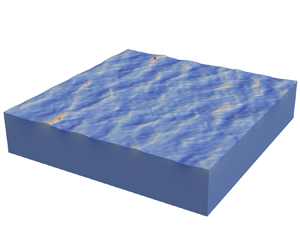
Figure 3. (a) Snapshots of the wave field development for the case of root-mean-square (r.m.s.) slope  $\sigma =0.153$. Breaking statistics are collected between
  $\omega _p t=124$ and
  $\omega _p t=149$ (indicated by the red box). (b) The wave energy spectrum on the frequency–wavenumber plane. The dotted white line is the linear dispersion relation of surface gravity waves
  $k=\omega ^2/g$. (c) Time evolution of the omni-directional wave spectrum
  $\phi (k)$, corresponding to the snapshots in (a). (d) Energy and
  $\sigma$ slope evolution of the wave field. Black line: evolution of wave energy (as the sum of potential and kinetic energy integrated over the whole field). Squares: the r.m.s. slope
  $\sigma$ of the four snapshots shown in (a); circles: the effective slope
  $k_pH_s$ of the four snapshots shown in (a). The breaking statistics are collected during the shaded time interval.
There are two commonly used measurements of the ‘slope’ of a broadband wave field: the effective slope  $k_pH_s$ and the root-mean-square (r.m.s.) slope
  $\sigma$. The effective slope
  $k_pH_s$ is essentially a measure of the wave field energy, where the significant wave height
  $H_s=4\langle \eta ^2\rangle ^{1/2}$ is related to the zeroth moment of the spectrum. The r.m.s. slope
  $\sigma$ is a measure of how ‘rough’ the wave field is and is related to the second moment of the spectrum. Here, we define the low-pass filtered steepness parameter
  $\mu (k)$ as
 \begin{equation} \mu^2(k) = \int_0^k k'^2\phi(k') \,{\rm d}k', \end{equation}
and  $\sigma$ is the asymptotic value of
  $\mu$ with a cutoff at the highest wavenumber we can numerically resolve
  $k_{max}$
 \begin{equation} \sigma^2 = \mu^2(k\to k_{max}) . \end{equation}
The value of  $k_{max}L_0$ is set to
  $2{\rm \pi} N_h/16$ based on the resolution convergence check (see Appendix B). Here,
  $N_h=N_x=N_y$ is the horizontal number of grid points and is 1024 for all the results reported. We note that another way of inferring the same quantity is from the variance of the slope distribution (see e.g. Cox & Munk Reference Cox and Munk1954; Munk Reference Munk2009).
Since there is no forcing mechanism, the total wave energy is slowly decaying (as shown in figure 3d). The Reynolds number defined by the peak wavelength  $\lambda _p$ is
  $Re_p=\lambda _p\sqrt {g\lambda _p}/\nu =3.17\times 10^7$, and the dissipation is Reynolds number independent. Instead, the dissipation is primarily due to the numerical gradient-limiter, and is of the order of magnitude of known dissipation due to breaking (Drazen et al. Reference Drazen, Melville and Lenain2008; Romero Reference Romero2019). We have also verified that the spatially and temporally averaged statistics are a good representation of the ensemble average, mainly because the domain size is large enough.
3.3. Procedure of breaking front detection and velocity measurement
The wave field evolves and breaking occurs intermittently in space and time. We detect the breaking fronts and their velocity, and construct the length of breaking crest distribution. The breaking fronts are defined geometrically as sharp enough ridges of the surface, as illustrated in figure 4(a). Given a surface elevation  $\eta (x,y)$ at one time instance, we find its Gaussian curvatures
  $\kappa _1$ and
  $\kappa _2$, and determine the location of the breaking fronts by the threshold
  $\kappa _2 < -3k_p$ (‘ridges’ of the
  $\eta$ surface), which works well across the different scales. The Gaussian curvatures are computed from the Hessian matrix
  $H(x,y)$ of surface elevation
  $\eta (x,y)$. Here,
  $H(x,y)$ is defined as
  $H(x,y) = \left [\begin {smallmatrix} \eta _{xx} & \eta _{yx} \\ \eta _{xy} & \eta _{yy} \end {smallmatrix}\right ]$, where
  $\eta _{xx}$,
  $\eta _{xy}$,
  $\eta _{yy}$ are the spatial second-order derivatives of
  $\eta$. The Gaussian curvatures
  $\kappa _1$,
  $\kappa _2$ (
 $|\kappa _1|<|\kappa _2|$) are the eigenvalues of this
  $2 \times 2$ matrix. (Since the matrix is symmetric, the eigenvalues are always real.)

Figure 4. (a) A 3-D rendering of the breaking wave field with the colour indicating the surface layer flow velocity. Inset shows the curvature of the breaking fronts as the detection criterion. (b) A more focused view taken from the dotted white square in figure 3(a). The arrows are showing the velocity magnitude and direction of each length element of the breaking fronts.
After the breaking regions (areas) are detected, we extract the breaking fronts (lines), shown in figure 4(b). Then, we use the surface layer Eulerian velocity ( $\boldsymbol {u}_{\boldsymbol {l}-\boldsymbol {1}}$ in figure 1) as an estimate of the Lagrangian velocity of the breaking fronts
  $\boldsymbol {c_b}$. The velocity is mapped on each discretised cell on the lines, which represents an element of length
  $L_0/N_x$. Figure 4(b) shows the mapped velocity magnitude and direction with arrows. The directionality of
  $\boldsymbol {c_b}$ is not discussed in this work, i.e. we only consider the magnitude
  $c_b=|\boldsymbol {c_b}|$. We have tested an alternative velocity mapping method by computing the correlation function between two consecutive images of the detected crests (similar to particle tracking velocimetry), and found no significant difference in the velocity magnitude detected or the resulting
  $\varLambda (c_b)$ distribution.
We follow Phillips (Reference Phillips1985), Kleiss & Melville (Reference Kleiss and Melville2010) and Sutherland & Melville (Reference Sutherland and Melville2013) and assume that  $c=c_b$; and we use a correspondence between the breaking front velocity and the underlying wavenumber through the dispersion relation
  $c=\sqrt {g/k}$. We note that observations have shown that
  $c_{b} = \alpha c$, where
  $\alpha$ is between 0.7 and 0.95 (Rapp & Melville Reference Rapp and Melville1990; Banner et al. Reference Banner, Zappa and Gemmrich2014; Romero Reference Romero2019), at least for large breakers. In the processing we filter out the smaller-scale breakers by imposing a filter
  $\eta (x,y) > 2.5 \langle \eta ^2\rangle ^{1/2}$. This means that only the large breakers with surface elevation above 2.5 r.m.s. value are included. As a result, no further corrections for the underlying long-wave orbital velocity are needed.
3.4. The  $\varLambda (c)$ distribution of different wave fields

We study the relation of the breaking statistics to the wave spectra. Figure 5(a) shows the (later quasi-steady stage) wave spectra for the various conditions, with variations in spectrum maxima larger than one order of magnitude, and described by power laws ranging from  $\phi (k)\propto k^{-2.5}$ to
  $\phi (k)\propto k^{-3}$. Although the energy near the peak frequency varies, a fixed level of saturation seems to be reached for the steeper cases with overlapping spectra in the
  $k^{-3}$ range.

Figure 5. Wave energy spectra of different steepnesses and their  $\varLambda (c)$ distribution. The colours correspond to different
  $\sigma$ slopes according to the colour bar. (a) The wave energy spectra during the breaking statistics collection time interval in non-dimensional form; the vertical grey line is
  $k_pL_0 = 10{\rm \pi}$. Darker colour indicates larger global slope
  $k_pH_s$ (see (b) for the values). (b) The correlation of r.m.s. slopes
  $\sigma$ and the global slopes
  $k_pH_s$ in the simulated cases. Crosses:
  $N=5$; circles:
  $N=2$; squares:
  $N=10$. (c) The non-dimensional breaking distribution
  $\varLambda (c)$ normalised by
  $c_p$ and
  $g$. Solid lines: directional spreading parameter
  $N=5$; dashed lines:
  $N=2$; dotted lines:
  $N=10$. (d) Proposed scaling for the
  $\varLambda (c)$ distribution using
  $\sigma$ and
  $c_p$. The pre-factor of the dotted line is 800.
As we see in figure 5(a), the value of  $\mu (k)$ plateaus due to the drop off of the spectrum. In weak nonlinear theories (such as wave-turbulence theory),
  $\mu < 0.1$ is used to justify the asymptotic expansions, at least for the range of
  $k$ considered (Zakharov et al. Reference Zakharov, L'vov and Falkovich1992). All the breaking cases in our simulation have
  $\mu$ close to or higher than 0.1, underlying the strong nonlinearity of the breaking wave field. The correlation between the two global slope parameters
  $k_pH_s$ (zeroth moment of the spectrum) and
  $\sigma$ (second moment of the spectrum) is shown by figure 5(b), which we caution is specific to the spectrum shape.
Figure 5(c) shows the breaking distribution  $\varLambda (c)$ for increasing
  $\sigma$ (and
  $k_p H_s$) values and the various directionalities. There is no breaking for the smallest
  $\sigma =0.0724$ case (
 $k_p H_s= 0.121$) (not shown in figure 5c). An increase in slope to
  $\sigma =0.0978$ (
 $k_p H_s=0.155$) and
  $\sigma =0.114$ (
 $k_p H_s= 0.173$) starts to generate breakers. The extent of breaking speeds is further increased for the steeper cases with
  $\sigma >0.101$, with a clear
  $\varLambda (c)\propto c^{-6}$ scaling up to around
  $0.9c_p$. This indicates that there exists a critical value of
  $\sigma$, below which the breaking wave field is not saturated, with the threshold expected to depend on the spectrum shape.
The shaded area in figure 5(c) spans the range of the breaker velocity between the peak  $\varLambda _{max}$ and
  $\varLambda (c)=0.01\varLambda _{max}$ (for the case of
  $\sigma =0.153$), where a power law scaling close to
  $\varLambda (c)\propto c^{-6}$ can be observed. The same range in the
  $k$-space is shaded in figure 5(a) as well. The upper limit of
  $\varLambda (c)=0.01\varLambda _{max}$ corresponds to a lower limit of
  $k\approx 4k_p$. Above that velocity, breakers near
  $k_p$ are very rare. We note that removing the filter of
  $\eta (x,y) > 2.5 \langle \eta \rangle ^{1/2}$ only changes the part of the
  $\varLambda (c)$ distribution left of the peak, but does not affect the part with
  $c$ larger than the peak. Similarly, further increasing the horizontal resolution would extend the move up and toward even smaller
  $c$, but the presented power law region is unchanged.
The  $\varLambda (c)$ distributions from spectra of different directionality
  $N$ are also shown with different lines (dashed lines indicate more spreading (
 $N=2$) and dotted lines less spreading (
 $N=10$)). For sufficiently steep cases (
 $\sigma > 0.101$), there is little difference in the
  $\varLambda (c)$ distribution between cases with different
  $N$, while for intermediate steepness (
 $\sigma = 0.85$ and
  $0.101$), there is a notable sensitivity to
  $N$. For the
  $N=10$ cases with more concentrated wave energy, there are overall more breaking events.
3.5. Wave-slope-based $\varLambda (c)$ scaling

The current set of numerical experiments with different wave spectra enables us to study the non-dimensional scaling of the breaking front distribution  $\varLambda (c)$, which has been a goal for many theoretical studies and observational campaigns. The goal is to predict the
  $\varLambda (c)$ distribution based on some global quantities of the spectrum, leveraging similarity of the breaking processes and the spectral shape.
The seminal work of Phillips (Reference Phillips1985) predicted a purely wind-based scaling  $\varLambda (c)\propto u_*^3 g c^{-6}$ through an energy balance argument (
 $u_*$ being the wind friction velocity). The wave action balance equation
  ${\rm d}[g\phi (k)/\omega ]/{\rm d}t = S_{nl}(k)+S_{in}(k)+S_{diss}(k)$ involves the following source terms: divergence of the nonlinear energy flux
  $S_{nl}$, wind input
  $S_{in}$ and dissipation due to breaking
  $S_{diss}$, written as (Phillips Reference Phillips1985)
 \begin{equation} S_{nl} \propto gk^{{-}3}B^3(k), \quad S_{in} \propto gk^{{-}3}\left(\frac{u_*}{c}\right)^2 B(k), \quad \text{and} \quad S_{diss} \propto gk^{{-}3} f(B(k)), \end{equation}
with the saturation  $B(k)=k^3\phi (k)$, and
  $f(B(k))$ a functional dependence solely on
  $B(k)$ (assuming that breaking and consequent dissipation ‘are the result of local excesses, however these excesses are produced’). The balance between
  $S_{nl}$ and
  $S_{diss}$ leads to
  $f(B)\propto B^3$, and therefore
 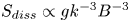 $S_{diss} \propto gk^{-3}B^{-3}$. The breaking front distribution
  $\varLambda (c)$ is then obtained by writing the equality between dissipation in the
  $k$-space and the
  $c$-space:
  $\epsilon (k)\,{\rm d}k = \epsilon (c)\,{\rm d}c$. The left-hand side is
  $\epsilon (k)\,{\rm d}k = (S_{diss}\omega ) \,{\rm d}k$; the right-hand side can be related to the fifth moment of
  $\varLambda (c)$ through a scaling argument
  $\epsilon (c)\,{\rm d}c = bg^{-1}c^5\varLambda (c)\,{\rm d}c$, where
  $b$ is a non-dimensional breaking parameter (Duncan Reference Duncan1981; Phillips Reference Phillips1985). Substituting a spectral shape of
  $\phi (k)\propto k^{-5/2}$ into the
  $S_{diss}$ would then lead to
  $\varLambda (c)\propto c^{-6}$. Considering the equilibrium range,
  $S_{nl} \propto S_{in}$ (Phillips Reference Phillips1985), gives
  $\phi (k) \propto u_*g^{-1/2}k^{-2.5}$, which leads to
 \begin{equation} \varLambda(c) \propto u_*^3gc^{{-}6}. \end{equation}
This wind-only scaling was, however, not confirmed by observations. To resolve this, later works (Sutherland & Melville Reference Sutherland and Melville2013; Deike & Melville Reference Deike and Melville2018, etc.) proposed modification of the scaling using a combination of wind speed, wave spectrum peak speed and significant wave height, in the form of
 \begin{equation} \varLambda(c)c_p^3 g^{{-}1} (c_p/u_*)^{1/2}\propto (c/\sqrt{g H_s})^{{-}6} ,\end{equation}
which significantly improved the collapse between data sets. This modification is empirical and is not based on clear physical reasoning.
In our numerical simulations, since we have no wind forcing, the breaking statistics are expected to scale only with the non-dimensional slope  $\sigma$ and spectrum peak speed
  $c_p$. Shown in figure 5(d), by rescaling
  $c$ using
  $\hat {c} = c/(\sigma c_p)$ and
  $\varLambda (c)$ using
  $\hat {\varLambda }(c) = \varLambda (c)c_p^3g^{-1}\sigma ^{-2}$, we are able to collapse the power law region well (for the sufficiently steep cases). The grey dashed line marks the scaling
 \begin{equation} \varLambda(c)c_p^3g^{{-}1}\sigma^{{-}2} \propto \left(c/(\sigma c_p)\right)^{{-}6} ,\end{equation}
and the corresponding pre-factor is 800. Alternatively, since the r.m.s. slope  $\sigma$ and the effective slope
  $k_pH_s$ are correlated, a scaling using
  $k_pH_s$ could be proposed. However, we have found that
  $\sigma$ works better than
  $k_pH_s$ as a scaling parameter for our simulated cases. The reason is likely because
  $\sigma$ as a global parameter is weighted favourably towards the larger
  $k$ part of the spectrum associated with breaking.
We note that, although most of the curves follow a  $\varLambda (c)\propto c^{-6}$ scaling, the two largest
  $\sigma$ cases exhibit a shallower slope closer to
  $c^{-5}$. We observe that these two cases have the
  $k^{-3}$ region of the energy spectrum extended further near the peak region, i.e. they have higher energy near the peak than the
  $k^{-2.5}$ ‘equilibrium’ shape, which results in more large breakers and therefore a shallower
  $\varLambda (c)$ slope. Similarly, a deficit of energy in the
  $k^{-2.5}$ ‘equilibrium range’ may result in a steeper slope of the power law region, which has been observed in some observational cases as well (Zappa et al. Reference Zappa, Banner, Schultz, Gemmrich, Morison, LeBel and Dickey2012). It is consistent with the argument in Phillips (Reference Phillips1985) that the
  $c^{-6}$ power law is a result of a choice of
  $k^{-2.5}$ spectrum shape.
3.6. Comparison with observations
We test our  $\sigma$-based scaling with observational data sets from field campaigns (Kleiss & Melville Reference Kleiss and Melville2010; Sutherland & Melville Reference Sutherland and Melville2013; Schwendeman, Thomson & Gemmrich Reference Schwendeman, Thomson and Gemmrich2014; Deike, Lenain & Melville Reference Deike, Lenain and Melville2017) where the spectrum information can be retrieved and re-analysed. The results are plotted in figure 6(a) and provide strong evidence that the
  $\sigma$-based scaling can be applied to rescale field data, without further need for wind information. The r.m.s. slope
  $\sigma _{obs}$ was computed from the observed wave spectra using (3.3), with a cutoff at
  $k_{max}=8 \ \text {m}^{-1}$, similar to that in the numerical cases. Data from Schwendeman & Thomson (Reference Schwendeman and Thomson2015) directly report
  $\sigma _{obs}$ from the second moment of the wave spectrum (up to 1 Hz, equivalent to
  $k\approx 4 \ \mathrm {m^{-1}}$). Data from Sutherland & Melville (Reference Sutherland and Melville2013) report the wave spectra measured up to
  $k=100 \ \text {m}^{-1}$ while Kleiss & Melville (Reference Kleiss and Melville2010) have a lower resolution so that we extended the spectra with a
  $k^{-3}$ tail up to
  $k=8\ \text {m}^{-1}$ to compute
  $\sigma _{obs}$. The reason why the Sutherland & Melville (Reference Sutherland and Melville2013) data set extends much further into the small
  $c$ range is that infrared imaging was used to capture very small breaking features. The main focus should be on the horizontal and vertical positions of the power law region. In general, the agreement of all three data sets within the numerically resolved range of
  $c$ gives confidence that the proposed
  $\sigma$-based scaling works well.

Figure 6. Comparison with observational data. (a) Rescaled  $\varLambda (c)$ following wave-slope-based scaling proposed by this work. (b) Rescaled
  $\varLambda (c)$ distribution following Sutherland & Melville (Reference Sutherland and Melville2013) with simplifications proposed by Deike (Reference Deike2022). (c) Whitecap coverage
  $W$ as a function of 10 m wind speed
  $U_{10}$.
The agreement with the two data sets shown in figure 6 is a promising sign that the proposed  $\sigma$-based scaling can provide a concise and physics-based prediction of
  $\varLambda (c)$ only using information of the wave energy spectra. However, there are a limited number of data sets that report both the wave energy spectra and
  $\varLambda (c)$, with more data sets being reported using empirical scaling such as (3.6). To compare with more data sets, and more importantly, to help understand the possible reasons behind the success of the empirical scaling, we perform the following re-analysis of the numerical data by inferring the wind forcing from the wave energy spectrum in the simulation.
Since there is no explicit wind forcing in our simulations, the information of wind speed and fetch/duration are encoded in the spectrum. We use the empirical (but very robust) fetch-limited relationships (Toba Reference Toba1972) that links the non-dimensional wave energy  $gH_s u_*^{-2}$ and the non-dimensional frequency
  $\omega _p g^{-1}u_*$ (wave age
  $u_*/c_p$) by
 \begin{equation} gH_s/u_*^2 = C (u_*/c_p)^{{-}3/2} , \end{equation}
where  $C$ is an order-1 constant. Using (3.8) it is straightforward to show that the scaling equation (3.7) with
  $\sigma \propto \sqrt {k_pH_s}$ is equivalent to the scaling from Sutherland & Melville (Reference Sutherland and Melville2013), since
  $k_pH_s \propto (c_p/u_*)^{1/2}$. After that we plot all the data sets using the empirical mixed wind-wave scaling in figure 6(b), and good agreement is observed. It indicates that the slope-based scaling is fully compatible with the mixed-wind-slope-based scalings, and the reason for that is the underlying fetch-limited relation. Note that the observational data are obtained from complex sea states, and do not necessarily have the same spectrum shape as the current numerical data. Some of the observational curves have been bin averaged according to the wave age
  $c/u_*$ and therefore shows less spreading.
Although we have shown that the proposed slope-based scaling is compatible with the empirical mixed-wind-wave-based one, it provides an alternative form that is both concise and fully interpretable. The wave field at a certain time and space is the result of the wind forcing history, and breaking is caused by excessive energy in the wave spectrum. For a mature and sufficiently steep wave field, breaking (particularly at large scale) is primarily dictated by the wave spectrum itself. Although we do caution that for younger and less steep wave fields, breaking can be more closely coupled to wind forcing. This can be seen from the deviation of curves with very small  $\sigma _{obs}$ in figure 6(a), and such conditions require further studies. An additional note is that the original derivation of the
  $\varLambda (c) \propto c^{-6}$ scaling is based on an energy dissipation argument, whereas in the numerical simulation, breaking is discussed in a purely kinematic sense. It remains to be investigated whether there is a simpler kinematic argument that would give rise to the same
  $\varLambda (c)$ distribution.
Finally, we can infer classic breaking metrics such as the whitecap coverage from our simulations and compare with more field data sets. The whitecap coverage  $W$ quantifies the fraction of the wave surface covered by white foam, and can be estimated through the second moment of
  $\varLambda (c)$ as
  $W=2{\rm \pi} \gamma g^{-1}\int c^2\varLambda (c) \,{\rm d}c$, where
  $\gamma$ is a dimensionless constant representing the ratio of breaking time to wave period (here,
  $\gamma = 0.56$ following Romero Reference Romero2019). Figure 6(b) shows
  $W$ as a function of the 10 m wind speed
  $U_{10}$;
  $U_{10}$ is estimated from
  $u_*$ (inferred using (3.8)) by the COARE parameterisation (Edson et al. Reference Edson, Jampana, Weller, Bigorre, Plueddemann, Fairall, Miller, Mahrt, Vickers and Hersbach2013), which is an empirical relation between
  $u_*$ and
  $U_{10}$. The modelled whitecap coverage falls within the scatter of recent data sets (Callaghan et al. Reference Callaghan, de Leeuw, Cohen and O'Dowd2008; Kleiss & Melville Reference Kleiss and Melville2010; Schwendeman & Thomson Reference Schwendeman and Thomson2015; Brumer et al. Reference Brumer, Zappa, Brooks, Tamura, Brown, Blomquist, Fairall and Cifuentes-Lorenzen2017).
4. Conclusion
We demonstrate that a novel multi-layer model (Popinet Reference Popinet2020) can be used to simulate free-surface waves with strong nonlinearity (and underwater turbulence) with reduced computational complexity compared with a two-phase Navier–Stokes solver. We apply it to study the breaking statistics associated with an ensemble of phase-resolved surface waves simulated in the physical space. We analyse the breaking front distribution introduced by Phillips (Reference Phillips1985), and find good agreement with field observations. The breaking distribution largely follows  $\varLambda (c) \propto c^{-6}$ even in the absence of wind input, and can be scaled by the wave r.m.s. slope, indicating that the universal breaking kinematics is primarily governed by the wave field itself, while the wind controls the development of the wave spectrum. The proposed scaling in terms of the r.m.s. slope is shown to apply to field data as well.
Our approach provides an unprecedented numerical framework to study breaking statistics for complex wave spectra, which could help to understand the breaking distribution in complex seas (in the presence of swell or currents) and complement existing modelling approaches such as Romero (Reference Romero2019). In addition to the physical discussion of breaking statistics, we demonstrate the capability of the multi-layer approach to solve highly nonlinear geophysical flows with strong vertical–horizontal anisotropy.
Funding
This work was supported by the National Science Foundation (Physical Oceanography) under Grant No. 2122042 to L.D., the High Meadows Environmental Institute Energy and Climate Grand Challenge, the NASA Ocean Vector Winds Science Team 22-OVWST22-0012 and the Cooperative Institute for Earth System Modeling between Princeton and the Geophysical Fluid Dynamics Laboratory (GFDL) NOAA. Computations were partially performed using the Extreme Science and Engineering Discovery Environment (XSEDE), which is supported by NSF Grant No. ACI-1053575; and on resources managed and supported by Princeton Research Computing, a consortium of groups including the Princeton Institute for Computational Science and Engineering and the Office of Information Technology's High Performance Computing Center and Visualization Laboratory at Princeton University. J.W. would also like to acknowledge the support of the Mary and Randall Hack ’69 Graduate Award received through the High Meadows Environmental Institute.
Declaration of interests
The authors report no conflict of interest.
Appendix A. Independence of the breaking statistics from the initial spectral shape
In the numerical simulation, we observe that the wave field dissipates the excessive energy and reaches a  $\phi (k)\propto k^{-3}$ quasi-steady energy spectrum independent of the initial spectral shape, as long as there is excessive energy initially. This is consistent with the idea of saturation, which dates back to Phillips (Reference Phillips1958). It explains that in the limit where the wave field is constrained by breaking, the spectrum should follow a
  $k^{-3}$ shape. As a result, the breaking statistics are not dependent on the choice of the initial spectral shape either (but still dependent on the steepness).
To demonstrate that the breaking front distribution results are not due to the choice of a particular initial spectral shape, we performed a simulation where the initial spectrum is a Gaussian distribution given by
 \begin{equation} \phi(k) = \frac{P}{s}\exp[{-}0.5(k-k_p)^2/s^2]. \end{equation}
In addition, we have considered a large variance  $s$ of the Gaussian distribution so that there is more energy in the shorter-wave range than a typical wind wave spectrum. We can see from figure 7 that the breaking model quickly dissipates the excessive energy and establishes a quasi-steady
  $k^{-3}$ distribution. After a quasi-steady spectrum is established, the breaking front distribution exhibits a power law similar to cases initialised with typical wind wave spectra, close to
  $\varLambda (c)\propto c^{-6}$. In figure 8 we compare the two initial Gaussian spectra cases with the other initial wind wave spectra cases. The correlation between
  $k_pH_s$ and
  $\sigma$ cases is spectrum shape dependent, but the proposed scaling for the
  $\varLambda (c)$ distribution works as well (because the spectra at late times are independent from the initial conditions) and the pre-factor is the same for all cases.

Figure 7. (a,b) Same as figure 3 but with the initially Gaussian spectra cases. A quasi-steady state spectrum is obtained after  $O(100\omega _p t)$, with a
  $k^{-3}$ shape. (c) The
  $\varLambda (c)$ distribution computed during different time windows in the quasi-steady regime.

Figure 8. Same as figure 5 comparing the initially Gaussian spectra cases and the wind wave initial spectra. Once a quasi-steady state is reached (due to breaking and loss of excess energy), the wave spectra and breaking distribution are comparable.
Appendix B. Resolution effects on the wave energy spectrum and breaking statistics
We show with the following verification cases that the wave energy spectra and breaking distributions are converged with respect to the horizontal number of grid point  $N_h$.
Case 1 and case 2 are two cases with different initial energy contents. Their spectrum evolution is shown in figure 9(a–c). The spectrum evolution is largely unchanged between horizontal grid point  $N_h=1024$ and 2048 for
  $k$ smaller than the resolution limit
  $k_{max}$, which is determined from 9(b,c) to be
  $2{\rm \pi} /(16\varDelta )$, where
  $\varDelta =L_0/N_h$ is the horizontal grid size. We use this value as our upper integration limit
  $k_{max}$ in
  $\sigma$ calculation.

Figure 9. Convergence between horizontal grid point  $N_h = 1024$ and 2048. (a–c) Wave energy spectra at
  $\omega _p t = 0,146,292$, respectively. The grey vertical lines indicate
  $k_{max}L_0$ for
  $N_h = 1024$ and 2048 respectively. (d) Energy evolution for case 1 and case 2 with varying horizontal grid points
  $N_h$. Solid lines: total energy; dashed lines: two times kinetic energy; dotted lines: two times potential energy. (e) Breaking distribution for case 1 and case 2 with varying horizontal grid points
  $N_h$. The grey vertical lines indicate the phase speed
  $k_{max}$ for
  $N_h = 1024$ and 2048, respectively.
The only discernible change when increasing the resolution is that there is a longer  $k^{-3}$ spectral tail in figure 9(b,c). Apart from the resolution effect, case 1 (less initial energy) has an earlier fall off than case 2 (more initial energy) because of the less frequent breaking events and therefore slower energy transfer to the large
  $k$ range. In a word, the extent of the
  $k^{-3}$ range is both breaking limited and resolution limited. Given enough time, case 1 will develop a
  $k^{-3}$ tail as well.
The energy decay for case 1 and case 2 is shown in figure 9(d). Between  $N_h=512$ and 1024 the difference is very significant, especially for the less steep case 1, therefore we use
  $N_h=1024$ for all the cases reported in the paper. There remains a small difference in energy dissipation between
  $N_h=1024$ and 2048, and the difference is mostly in the kinetic energy, which indicates a discrepancy mostly in the underwater turbulence.
As a result of the convergence in the wave energy spectra, there is a convergence in the breaking distribution  $\varLambda (c)$ shown in 9(e), for
  $c$ that are larger than the resolution limit. Again this indicates that the kinematics of breaking is a direct result of the wave energy spectrum, but not strongly coupled to its dynamic effects such as breaking-induced dissipation.


 Open access