2 Problem formulation and main results

In this paper we consider Maxwell equations for a three-dimensional two-component periodic dielectric composite when the dielectric properties of the constituent materials exhibit a high degree of contrast. We assume that the reference cell $Q:= [\!0,1\!)^{3}$ contains an inclusion $Q_{0},$ which is an open set with sufficiently smooth boundary. We also assume that the “matrix” $Q_{1}:=Q\backslash \overline{Q_{0}}$ is simply connected Lipschitz set.

We consider a composite with high contrast in the dielectric permittivity $\unicode[STIX]{x1D716}_{\unicode[STIX]{x1D702}}=\unicode[STIX]{x1D716}_{\unicode[STIX]{x1D702}}(x/\unicode[STIX]{x1D702})$ at points $x\in \unicode[STIX]{x1D702}(Q_{1}+m)$ , $m\in \mathbb{Z}^{3},$ and $x\in \unicode[STIX]{x1D702}(Q_{0}+m),$ $m\in \mathbb{Z}^{3},$ namely

$$\begin{eqnarray}\unicode[STIX]{x1D716}_{\unicode[STIX]{x1D702}}(y)=\left\{\begin{array}{@{}ll@{}}\unicode[STIX]{x1D702}^{-2}\unicode[STIX]{x1D716}_{0}(y), & y\in Q_{0},\\ \unicode[STIX]{x1D716}_{1}(y), & y\in Q_{1},\end{array}\right.\end{eqnarray}$$

where $\unicode[STIX]{x1D702}\in (0,1)$ is the period and $\unicode[STIX]{x1D716}_{0}$ , $\unicode[STIX]{x1D716}_{1}$ are continuously differentiable $Q$ -periodic positive-definite scalar functions.

We also assume moderate contrast in the magnetic permeability, and for simplicity of exposition we shall set $\unicode[STIX]{x1D707}\equiv 1$ . We consider the open cube $\mathbb{T}:=(0,T)^{3}$ and those values of the parameter $\unicode[STIX]{x1D702}$ for which $T/\unicode[STIX]{x1D702}\in \mathbb{N}.$ By rescaling the spatial variable (which can also be viewed as non-dimensionalization) we assume that $T=1$ and that $\unicode[STIX]{x1D702}^{-1}\in \mathbb{N}.$ We shall study the behaviour of the magnetic component $H^{\unicode[STIX]{x1D702}}$ of the electromagnetic wave of frequency $\unicode[STIX]{x1D714}$ propagating through the domain $\mathbb{T}$ occupied by a dielectric material with permittivity $\unicode[STIX]{x1D716}_{\unicode[STIX]{x1D702}}(x/\unicode[STIX]{x1D702}).$ More precisely, we consider pairs $(\unicode[STIX]{x1D714}_{\unicode[STIX]{x1D702}},H^{\unicode[STIX]{x1D702}})\in \mathbb{R}_{+}\times [H_{\#}^{1}(\mathbb{T})]^{3}$ satisfying the system of equations

(2.1) $$\begin{eqnarray}\text{curl}_{}\biggl(\unicode[STIX]{x1D716}_{\unicode[STIX]{x1D702}}^{-1}\biggl(\frac{\cdot }{\unicode[STIX]{x1D702}}\biggr)\text{curl}_{}\,H^{\unicode[STIX]{x1D702}}\biggr)=\unicode[STIX]{x1D714}_{\unicode[STIX]{x1D702}}^{2}H^{\unicode[STIX]{x1D702}}.\end{eqnarray}$$

Notice that solutions of (2.1) are automatically solenoidal, that is, $\text{div}\,H^{\unicode[STIX]{x1D702}}=0$ .

We seek solutions to the above problem in the form of an asymptotic expansion

(2.2) $$\begin{eqnarray}\displaystyle \begin{array}{@{}c@{}}\displaystyle H^{\unicode[STIX]{x1D702}}(x)=H^{0}\biggl(x,\frac{x}{\unicode[STIX]{x1D702}}\biggr)+\unicode[STIX]{x1D702}H^{1}\biggl(x,\frac{x}{\unicode[STIX]{x1D702}}\biggr)+\unicode[STIX]{x1D702}^{2}H^{2}\biggl(x,\frac{x}{\unicode[STIX]{x1D702}}\biggr)+\cdots \,,\\ \displaystyle \unicode[STIX]{x1D714}_{\unicode[STIX]{x1D702}}=\unicode[STIX]{x1D714}+\unicode[STIX]{x1D702}\unicode[STIX]{x1D714}_{1}+\unicode[STIX]{x1D702}^{2}\unicode[STIX]{x1D714}_{2}+\cdots \,,\end{array} & & \displaystyle\end{eqnarray}$$

where the vector functions $H^{j}(x,y)$ , $j=0,1,2,\ldots ,$ are $Q$ -periodic in the variable $y$ . (Note that the terms of order $O(\unicode[STIX]{x1D702})$ and higher in the expansion for $\unicode[STIX]{x1D714}_{\unicode[STIX]{x1D702}}$ will be of no importance in what follows.) Substituting (2.2) into (2.1) and gathering the coefficients for each power of the parameter $\unicode[STIX]{x1D702}$ results in a system of recurrence relations for $H^{j},$ $j=0,1,2,\ldots$  ; see §4. In particular, the function $H^{0}$ is an eigenfunction of a limit (“homogenized”) system of partial differential equations, as described in the following theorem.

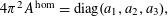
Theorem 2.1. Consider the constant matrix

$$\begin{eqnarray}A^{\text{hom}}:=\int _{Q_{1}}\unicode[STIX]{x1D716}_{1}^{-1}(y)(\text{curl}\,N(y)+I)\,dy,\end{eqnarray}$$

where the vector function $N$ is a solution to the “unit-cell problem”

(2.3) $$\begin{eqnarray}\displaystyle \begin{array}{@{}c@{}}\displaystyle \text{curl}(\unicode[STIX]{x1D716}_{1}^{-1}[\text{curl}\,N+I])=0\quad \text{in }Q_{1},\\ \displaystyle \unicode[STIX]{x1D716}_{1}^{-1}(\text{curl}\,N+I)\times n=0\quad \text{on }\unicode[STIX]{x2202}Q_{0},N\text{ is }Q\text{-periodic},\end{array} & & \displaystyle\end{eqnarray}$$

in which $n$ is the exterior normal to $\unicode[STIX]{x2202}Q_{0}$ .

Suppose that $\unicode[STIX]{x1D714}\in \mathbb{R}_{+}$ and $H^{0}(x,y)=u(x)+\unicode[STIX]{x1D6FB}_{y}v(x,y)+z(x,y),$ where the tripletFootnote ¹ $(u,v,z)\in [H_{\#\text{curl}}^{1}(\mathbb{T})]^{3}\times L^{2}(\mathbb{T};H_{\#}^{2}(Q))\times [L^{2}(\mathbb{T};H_{0}^{1}(Q_{0}))]^{3}$ satisfies the system of equations

(2.4) $$\begin{eqnarray}\displaystyle & \displaystyle \text{curl}_{x}(A^{\text{hom}}\,\text{curl}_{x}\,u(x))=\unicode[STIX]{x1D714}^{2}\biggl(u(x)+\int _{Q_{0}}z(x,y)\,dy\biggr),\quad x\in \mathbb{T}, & \displaystyle\end{eqnarray}$$

(2.5) $$\begin{eqnarray}\displaystyle & \displaystyle \text{div}_{y}(\unicode[STIX]{x1D6FB}_{y}v(x,y)+z(x,y))=0,\quad (x,y)\in \mathbb{T}\times Q, & \displaystyle\end{eqnarray}$$

(2.6) $$\begin{eqnarray}\displaystyle \begin{array}{@{}c@{}}\displaystyle \text{curl}_{y}(\unicode[STIX]{x1D716}_{0}^{-1}(y)\,\text{curl}_{y}\,z(x,y))=\unicode[STIX]{x1D714}^{2}(u(x)+\unicode[STIX]{x1D6FB}_{y}v(x,y)+z(x,y)),\\ \displaystyle \qquad \qquad \qquad (x,y)\in \mathbb{T}\times Q_{0}.\end{array} & & \displaystyle\end{eqnarray}$$

Then:

1. (1) There exists at least one eigenfrequency $\unicode[STIX]{x1D714}_{\unicode[STIX]{x1D702}}$ for (2.1) such that

   (2.7) $$\begin{eqnarray}|\unicode[STIX]{x1D714}_{\unicode[STIX]{x1D702}}-\unicode[STIX]{x1D714}|<C\unicode[STIX]{x1D702},\end{eqnarray}$$
   with an $\unicode[STIX]{x1D702}$ -independent constant $C>0$ .

2. (2) Consider the finite-dimensional vector space

   $$\begin{eqnarray}X_{\unicode[STIX]{x1D702}}:=\text{span}\{H^{\unicode[STIX]{x1D702}}:\text{(2.1) holds, where }\unicode[STIX]{x1D714}_{\unicode[STIX]{x1D702}}\text{ satisfies (2.7)}\}.\end{eqnarray}$$
   There exists an $\unicode[STIX]{x1D702}$ -independent constant $\widehat{C}>0$ such that
   $$\begin{eqnarray}\inf _{H\in X_{\unicode[STIX]{x1D702}}}\biggl\|H^{0}\biggl(\cdot ,\frac{\cdot }{\unicode[STIX]{x1D702}}\biggr)-H(\cdot )\biggr\|_{L^{2}(\mathbb{T})}<\widehat{C}\unicode[STIX]{x1D702}.\end{eqnarray}$$

The matrix $A^{\text{hom}}$ is described by solutions to certain degenerate “cell problems”, as follows. Consider the spaces

(2.8) $$\begin{eqnarray}V:=\{v\in [H_{\#}^{1}(Q)]^{3}:\text{curl}_{}\,v=0\text{ in }Q_{1}\}\end{eqnarray}$$

and $V^{\bot },$ the orthogonal complement of $V$ in $[H_{\#}^{1}(Q)]^{3}$ with respect to the equivalent $H^{1}(Q)$ -norm

$$\begin{eqnarray}\Vert v\Vert _{H^{1}(Q)}:=\biggl(\biggl|\int _{Q}v\biggr|^{2}+\int _{Q}|\unicode[STIX]{x1D6FB}v|^{2}\biggr)^{1/2},\end{eqnarray}$$

associated with the inner product

$$\begin{eqnarray}(v,w)_{H^{1}(Q)}:=\biggl(\int _{Q}v\biggr)\cdot \biggl(\int _{Q}w\biggr)+\int _{Q}\unicode[STIX]{x1D6FB}v\cdot \unicode[STIX]{x1D6FB}w.\end{eqnarray}$$

Then

(2.9) $$\begin{eqnarray}A^{\text{hom}}\unicode[STIX]{x1D709}=\int _{Q}\unicode[STIX]{x1D716}_{1}^{-1}(\text{curl}\,N_{\unicode[STIX]{x1D709}}+\unicode[STIX]{x1D709}),\quad \unicode[STIX]{x1D709}\in \mathbb{R}^{3},\end{eqnarray}$$

where $N_{\unicode[STIX]{x1D709}}$ , $\unicode[STIX]{x1D709}\in \mathbb{R}^{3}$ , is the unique (weak) solution in $V^{\bot }$ to the problem (2.3), that is,

(2.10) $$\begin{eqnarray}\int _{Q}\unicode[STIX]{x1D716}_{1}^{-1}(\text{curl}_{\,}N_{\unicode[STIX]{x1D709}}+\unicode[STIX]{x1D709})\cdot \text{curl}_{\,}\unicode[STIX]{x1D711}=0\quad \text{for all }\unicode[STIX]{x1D711}\in V^{\bot }.\end{eqnarray}$$

Existence and uniqueness of $N_{\unicode[STIX]{x1D709}}$ are discussed in §4.

Notice that

(2.11) $$\begin{eqnarray}A^{\text{hom}}\unicode[STIX]{x1D709}\cdot \unicode[STIX]{x1D709}=\min _{U\in [H_{\#}^{1}(Q)]^{3}}\int _{Q_{1}}\unicode[STIX]{x1D716}_{1}^{-1}(\text{curl}\,U+\unicode[STIX]{x1D709})\cdot (\text{curl}\,U+\unicode[STIX]{x1D709}),\quad \unicode[STIX]{x1D709}\in \mathbb{R}^{3}.\end{eqnarray}$$

Indeed, for the functional

$$\begin{eqnarray}F_{\unicode[STIX]{x1D709}}(U):=\int _{Q_{1}}\unicode[STIX]{x1D716}_{1}^{-1}(\text{curl}\,U+\unicode[STIX]{x1D709})\cdot (\text{curl}\,U+\unicode[STIX]{x1D709}),\end{eqnarray}$$

we find $F_{\unicode[STIX]{x1D709}}(U)=F_{\unicode[STIX]{x1D709}}(P_{V^{\bot }}U)$ for all $U\in [H_{\#}^{1}(Q)]^{3}$ , where $P_{V^{\bot }}$ is the orthogonal projection onto $V^{\bot }$ . Therefore, without loss of generality, $F_{\unicode[STIX]{x1D709}}$ can be minimized on $V^{\bot }$ for which (2.10) is the corresponding Euler–Lagrange equation.

The variational formulation (2.11) allows one to obtain a representation for the matrix $\unicode[STIX]{x1D716}_{\text{stiff}}^{\text{hom}}$ such that

(2.12) $$\begin{eqnarray}\displaystyle \unicode[STIX]{x1D716}_{\text{stiff}}^{\text{hom}}\unicode[STIX]{x1D709}\cdot \unicode[STIX]{x1D709}:=\inf _{\substack{ u\in H_{\#}^{1}(Q), \\ \unicode[STIX]{x1D6FB}u=-\unicode[STIX]{x1D709}\text{in }Q_{0}}}\int _{Q_{1}}\unicode[STIX]{x1D716}_{1}(\unicode[STIX]{x1D6FB}u+\unicode[STIX]{x1D709})\cdot (\unicode[STIX]{x1D6FB}u+\unicode[STIX]{x1D709}),\quad \unicode[STIX]{x1D709}\in \mathbb{R}^{3}, & & \displaystyle\end{eqnarray}$$

which arises in the homogenization of periodic problems with stiff inclusions; see [Reference Jikov, Kozlov and Oleinik5, §3.2].Footnote ²

Indeed, as shown in [Reference Jikov, Kozlov and Oleinik5, p. 101], the following representation holds:

(2.13) $$\begin{eqnarray}(\unicode[STIX]{x1D716}_{\text{stiff}}^{\text{hom}})^{-1}\unicode[STIX]{x1D709}\cdot \unicode[STIX]{x1D709}=\inf _{\substack{ v\in [L^{2}(Q)]_{\text{sol}}^{3}, \\ \langle v\rangle =0}}\int _{Q_{1}}\unicode[STIX]{x1D716}_{1}^{-1}(v+\unicode[STIX]{x1D709})\cdot (v+\unicode[STIX]{x1D709}),\quad \unicode[STIX]{x1D709}\in \mathbb{R}^{3}.\end{eqnarray}$$

Notice that for each vector $v$ in (2.13) there exists $U_{v}\in [H_{\#}^{1}(Q)]^{3}$ such that $v=\text{curl}\,U_{v}$ (see [Reference Jikov, Kozlov and Oleinik5, pp. 6–7]), and hence

$$\begin{eqnarray}\int _{Q_{1}}\unicode[STIX]{x1D716}_{1}^{-1}(v+\unicode[STIX]{x1D709})\cdot (v+\unicode[STIX]{x1D709})=\int _{Q_{1}}\unicode[STIX]{x1D716}_{1}^{-1}(\text{curl}(P_{V^{\bot }}U_{v})+\unicode[STIX]{x1D709})\cdot (\text{curl}(P_{V^{\bot }}U_{v})+\unicode[STIX]{x1D709}).\end{eqnarray}$$

It follows that for all $\unicode[STIX]{x1D709}\in \mathbb{R}^{3}$ one has

$$\begin{eqnarray}\displaystyle (\unicode[STIX]{x1D716}_{\text{stiff}}^{\text{hom}})^{-1}\unicode[STIX]{x1D709}\cdot \unicode[STIX]{x1D709} & = & \displaystyle \inf _{U\in [H_{\#}^{1}(Q)]^{3}}\int _{Q_{1}}\unicode[STIX]{x1D716}_{1}^{-1}(\text{curl}(P_{V^{\bot }}U)+\unicode[STIX]{x1D709})\cdot (\text{curl}(P_{V^{\bot }}U)+\unicode[STIX]{x1D709})\nonumber\\ \displaystyle & = & \displaystyle A^{\text{hom}}\unicode[STIX]{x1D709}\cdot \unicode[STIX]{x1D709}.\nonumber\end{eqnarray}$$

3 On the spectrum of the limit problem

In this section we study the set of values $\unicode[STIX]{x1D714}^{2}$ such that there exists a non-trivial triple $(u,v,z)$ solving the two-scale limit spectral problem (2.4)–(2.6).

3.1 Equivalent formulation and spectral decomposition of the limit problem

Let $G$ be the Green function for the scalar periodic Laplacian, that is, for all $y\in Q$ , one has

$$\begin{eqnarray}-\unicode[STIX]{x1D6E5}G(y)=\unicode[STIX]{x1D6FF}_{0}(y)-1,\quad y\in Q,G\text{ is }Q\text{-periodic},\end{eqnarray}$$

where $\unicode[STIX]{x1D6FF}_{0}$ is the Dirac delta function supported at zero, on $Q$ considered as a torus. Then, as the functions $v$ , $z$ solve (2.5), we have $v(x,\cdot )=G\ast (\text{div}_{y}\,z)(x,\cdot ),$ and (2.6) takes the form

(3.1) $$\begin{eqnarray}\displaystyle & & \displaystyle \text{curl}_{y}(\unicode[STIX]{x1D716}_{0}^{-1}(y)\text{curl}_{y}\,z(x,y))\nonumber\\ \displaystyle & & \displaystyle \quad =\unicode[STIX]{x1D714}^{2}\biggl(u(x)+\unicode[STIX]{x1D6FB}_{y}\int _{Q_{0}}G(y-y^{\prime })\,\text{div}_{y^{\prime }}\,z(x,y^{\prime })\,dy^{\prime }+z(x,y)\biggr),\nonumber\\ \displaystyle & & \displaystyle \qquad (x,y)\in \mathbb{T}\times Q_{0}.\end{eqnarray}$$

For the case $\unicode[STIX]{x1D714}=0$ the set of solutions $z$ to (3.1) subject to the condition $z(x,y)=0$ , $x\in \mathbb{T},$ $y\in \unicode[STIX]{x2202}Q_{0},$ is clearly given by $L^{2}(\mathbb{T},{\mathcal{H}}_{0}),$ where ${\mathcal{H}}_{0}:=\{u\in [H_{0}^{1}(Q_{0})]^{3}:\text{curl}\,u=0\}.$

Further, for $\unicode[STIX]{x1D714}\neq 0,$ as (3.1) is linear in $u(x)$ and $\text{curl}_{y}\unicode[STIX]{x1D6FB}_{y}=0$ , we set

(3.2) $$\begin{eqnarray}\unicode[STIX]{x1D6FB}_{y}\int _{Q_{0}}G(y-y^{\prime })\,\text{div}_{y^{\prime }}\,z(x,y^{\prime })\,dy^{\prime }+z(x,y)=\unicode[STIX]{x1D714}^{2}B(y)u(x),\end{eqnarray}$$

where $B$ is a $3\times 3$ matrix function whose column vectors $B^{j}$ , $j=1,2,3,$ are solutions in $[H_{\#}^{1}(Q)]^{3}$ to the system

(3.3) $$\begin{eqnarray}\displaystyle \text{curl}_{}(\unicode[STIX]{x1D716}_{0}^{-1}\,\text{curl}_{}B^{j}) & = & \displaystyle e_{j}+\unicode[STIX]{x1D714}^{2}B^{j}\quad \text{in }Q_{0},\end{eqnarray}$$

(3.4) $$\begin{eqnarray}\displaystyle \text{curl}\,B^{j} & = & \displaystyle 0\quad \text{in }Q_{1},\end{eqnarray}$$

(3.5) $$\begin{eqnarray}\displaystyle \text{div}\,B^{j} & = & \displaystyle 0\quad \text{in }Q,\end{eqnarray}$$

(3.6) $$\begin{eqnarray}\displaystyle a(B^{j}) & = & \displaystyle 0,\end{eqnarray}$$

where $e_{j}$ , $j=1,2,3,$ are the Euclidean basis vectors and $a(B^{j})$ is the “circulation” of $B^{j},$ that is defined as the continuous extension, in the sense of the $H^{1}$ norm, of the map given by $a(\unicode[STIX]{x1D719})_{i}=\int _{0}^{1}\unicode[STIX]{x1D719}_{i}(te_{i})\,dt$ , $i=1,2,3$ , for $\unicode[STIX]{x1D719}\in [C^{\infty }(Q)]^{3}$ . Note that, since $B^{j}\in [H^{1}(Q)]^{3}$ , equation (3.4) implies $\unicode[STIX]{x1D716}_{0}^{-1}\text{curl}_{}\,B^{j}\times n|_{-}=0$ on $\unicode[STIX]{x2202}Q_{0}$ . Furthermore, the system (3.3)–(3.6) implies the variational problem of finding $B^{j}\in [H_{\#}^{1}(Q)]^{3},$ subject to the constraints (3.4)–(3.6), such that the following identity holds:

(3.7) $$\begin{eqnarray}\displaystyle & & \displaystyle \int _{Q_{0}}\unicode[STIX]{x1D716}_{0}^{-1}\,\text{curl}\,B^{j}\cdot \text{curl}\,\unicode[STIX]{x1D711}\nonumber\\ \displaystyle & & \displaystyle \quad =\int _{Q}e_{j}\cdot \unicode[STIX]{x1D711}+\unicode[STIX]{x1D714}^{2}\int _{Q}B^{j}\cdot \unicode[STIX]{x1D711}\quad \text{for all }\unicode[STIX]{x1D711}\in [H_{\#}^{1}(Q)]^{3}\text{ satisfying (3.4){-}(3.6).}\nonumber\\ \displaystyle & & \displaystyle\end{eqnarray}$$

Indeed, functions $\unicode[STIX]{x1D711}\in [H_{\#}^{1}(Q)]^{3}$ which satisfy (3.4) and (3.6) admit (see Lemma 4.1 below) the representation $\unicode[STIX]{x1D711}=\unicode[STIX]{x1D6FB}p+\unicode[STIX]{x1D713}$ , $p\in H_{\#}^{2}(Q)$ , $\unicode[STIX]{x1D713}\in [H_{0}^{1}(Q_{0})]^{3}$ . Therefore, it is straightforward to show (3.7) holds for $\unicode[STIX]{x1D711}=\unicode[STIX]{x1D713}$ if and only if (3.3) holds. Similarly, one can show (3.7) holds for $\unicode[STIX]{x1D711}=\unicode[STIX]{x1D6FB}p$ if and only if (3.5) holds.

Substituting the representation (3.2) into (2.4) and using the fact that

$$\begin{eqnarray}\int _{Q}(\unicode[STIX]{x1D6FB}_{y^{\prime }}G\ast (\text{div}_{y}\,z)(x,y^{\prime })+z(x,y^{\prime }))\,dy^{\prime }=\int _{Q_{0}}z(x,y)\,dy,\end{eqnarray}$$

leads to the operator-pencil spectral problem

(3.8) $$\begin{eqnarray}\text{curl}_{}(A^{\text{hom}}\,\text{curl}_{}\,u(x))=\unicode[STIX]{x1D6E4}(\unicode[STIX]{x1D714})u(x),\quad x\in \mathbb{T},\end{eqnarray}$$

where $\unicode[STIX]{x1D6E4}$ is a matrix-valued function that vanishes at $\unicode[STIX]{x1D714}=0,$ and for $\unicode[STIX]{x1D714}\neq 0$ has elements

(3.9) $$\begin{eqnarray}\unicode[STIX]{x1D6E4}_{ij}(\unicode[STIX]{x1D714})=\unicode[STIX]{x1D714}^{2}\biggl(\unicode[STIX]{x1D6FF}_{ij}+\unicode[STIX]{x1D714}^{2}\int _{Q}B_{i}^{j}\biggr),\quad i,j=1,2,3.\end{eqnarray}$$

We denote by ${\mathcal{H}}_{1}$ the space of vector fields in $[H_{\#}^{1}(Q)]^{3}$ that satisfy conditions (3.4)–(3.6). It can be shownFootnote ³ that there exist countably many pairs $(\unicode[STIX]{x1D6FC}^{k},r^{k})\in \mathbb{R}\times {\mathcal{H}}_{1}$ such that $\Vert r^{k}\Vert _{[L^{2}(Q)]^{3}}=1$ and

$$\begin{eqnarray}\text{curl}_{}(\unicode[STIX]{x1D716}_{0}^{-1}\,\text{curl}_{}\,r^{k})=\unicode[STIX]{x1D6FC}^{k}r^{k}\quad \text{in }Q_{0}.\end{eqnarray}$$

Moreover, the sequence $(r^{k})_{k\in \mathbb{N}}$ can be chosen to form an orthonormal basis of the closure $\overline{{\mathcal{H}}}_{1}$ of ${\mathcal{H}}_{1}$ in $[L^{2}(Q)]^{3}$ and, upon a suitable rearrangement, one has

$$\begin{eqnarray}0<\unicode[STIX]{x1D6FC}^{1}\leqslant \unicode[STIX]{x1D6FC}^{2}\leqslant \cdots \leqslant \unicode[STIX]{x1D6FC}^{k}\leqslant \cdots \stackrel{k\rightarrow \infty }{\longrightarrow }\infty .\end{eqnarray}$$

Performing a decompositionFootnote ⁴ of the functions $B^{j}$ , $j=1,2,3,$ with respect to the above basis yields

$$\begin{eqnarray}B_{i}^{j}=\mathop{\sum }_{k=1}^{\infty }\frac{\int _{Q}r_{j}^{k}}{\unicode[STIX]{x1D6FC}^{k}-\unicode[STIX]{x1D714}^{2}}r_{i}^{k},\quad \unicode[STIX]{x1D714}^{2}\notin \cup \,\{\unicode[STIX]{x1D6FC}^{k}\}_{k=1}^{\infty },\end{eqnarray}$$

where $r_{j}^{k}$ , $j=1,2,3,$ are the components of the vector $r^{k},$ $k\in \mathbb{N}$ .

Consider the functions $\unicode[STIX]{x1D719}^{k}\in [H_{0}^{1}(Q_{0})]^{3}$ , $k\in \mathbb{N},$ that solve the non-local problems

(3.10) $$\begin{eqnarray}\displaystyle & & \displaystyle \text{curl}_{}(\unicode[STIX]{x1D716}_{0}^{-1}(y)\,\text{curl}_{}\unicode[STIX]{x1D719}^{k}(y))\nonumber\\ \displaystyle & & \displaystyle \quad =\unicode[STIX]{x1D6FC}^{k}\biggl(\unicode[STIX]{x1D6FB}\int _{Q_{0}}G(y-y^{\prime })\,\text{div}\,\unicode[STIX]{x1D719}^{k}(y^{\prime })\,dy^{\prime }+\unicode[STIX]{x1D719}^{k}(y)\biggr),\quad y\in Q_{0},\end{eqnarray}$$

and satisfy the orthonormality conditions

$$\begin{eqnarray}\int _{Q_{0}}\int _{Q_{0}}(\unicode[STIX]{x1D6FB}^{2}G(y-y^{\prime })+I)\unicode[STIX]{x1D719}^{j}(y)\cdot \overline{\unicode[STIX]{x1D719}^{k}(y^{\prime })}\,dy\,dy^{\prime }=\unicode[STIX]{x1D6FF}_{jk},\quad j,k=1,2,\ldots ,\end{eqnarray}$$

where $\unicode[STIX]{x1D6FB}^{2}G$ is the Hessian matrix of $G.$ Using the formula

$$\begin{eqnarray}r^{k}(y)=\unicode[STIX]{x1D6FB}\int _{Q_{0}}G(y-y^{\prime })\,\text{div}\,\unicode[STIX]{x1D719}^{k}(y^{\prime })\,dy^{\prime }+\unicode[STIX]{x1D719}^{k}(y),\quad y\in Q,\end{eqnarray}$$

we obtain the following representation for $\unicode[STIX]{x1D6E4}$ :

(3.11) $$\begin{eqnarray}\displaystyle \unicode[STIX]{x1D6E4}_{ij}(\unicode[STIX]{x1D714}) & = & \displaystyle \unicode[STIX]{x1D714}^{2}\unicode[STIX]{x1D6FF}_{ij}+\unicode[STIX]{x1D714}^{4}\mathop{\sum }_{k=1}^{\infty }\frac{(\int _{Q_{0}}\unicode[STIX]{x1D719}_{i}^{k})(\int _{Q_{0}}\unicode[STIX]{x1D719}_{j}^{k})}{\unicode[STIX]{x1D6FC}^{k}-\unicode[STIX]{x1D714}^{2}},\nonumber\\ \displaystyle & & \displaystyle i,j=1,2,3,\quad \unicode[STIX]{x1D714}^{2}\notin \{0\}\cup \{\unicode[STIX]{x1D6FC}^{k}\}_{k=1}^{\infty }.\end{eqnarray}$$

3.2 Analysis of the limit spectrum

Consider the Fourier expansion for the function $u$ in (3.8):

$$\begin{eqnarray}u(x)=\mathop{\sum }_{m\in \mathbb{Z}^{3}}\exp (2\unicode[STIX]{x1D70B}\text{i}m\cdot x)\hat{u} (m),\qquad \hat{u} (m):=\int _{\mathbb{T}}\exp (-2\unicode[STIX]{x1D70B}\text{i}m\cdot x)u(x)\,dx,\end{eqnarray}$$

where the integral is taken componentwise. As $u$ solves (3.8), the coefficients $\hat{u} (m)$ satisfy the equation

(3.12) $$\begin{eqnarray}{\mathcal{M}}(m)\hat{u} (m)=\unicode[STIX]{x1D6E4}(\unicode[STIX]{x1D714})\hat{u} (m),\quad m\in \mathbb{Z}^{3},\end{eqnarray}$$

with the matrix-valued function ${\mathcal{M}}$ given by

$$\begin{eqnarray}\displaystyle {\mathcal{M}}_{lp}(m) & = & \displaystyle 4\unicode[STIX]{x1D70B}^{2}\mathop{\sum }_{i,j,s,t=1}^{3}\unicode[STIX]{x1D700}_{ils}m_{s}A_{ij}^{\text{hom}}\unicode[STIX]{x1D700}_{jpt}m_{t}\nonumber\\ \displaystyle & = & \displaystyle 4\unicode[STIX]{x1D70B}^{2}(e_{l}\times m)\cdot A^{\text{hom}}(e_{p}\times m),\quad m\in \mathbb{Z}^{3},l,p=1,2,3,\nonumber\end{eqnarray}$$

where $e_{j}$ , $j=1,2,3$ are the Euclidean basis vectors. Here $\unicode[STIX]{x1D700}$ is the Levi-Civita symbol:

$$\begin{eqnarray}\unicode[STIX]{x1D700}_{jkl}=\left\{\begin{array}{@{}ll@{}}1, & (jkl)=(123),(231),(312),\\ -1, & (jkl)=(132),(321),(213),\\ 0 & \text{otherwise}.\end{array}\right.\end{eqnarray}$$

Notice that, for all $m\in \mathbb{Z}^{3}\setminus \{0\},$ zero is a simple eigenvalue of ${\mathcal{M}}(m)$ with eigenvector $m,$ and since the matrix $A^{\text{hom}}$ is symmetric and positive definite, the values of ${\mathcal{M}}$ are also symmetric and positive definite on vectors $\unicode[STIX]{x1D709}$ such that $\unicode[STIX]{x1D709}\cdot m=0.$ In particular, for all $m\in \mathbb{Z}^{3},$ one has

(3.13) $$\begin{eqnarray}\displaystyle \unicode[STIX]{x1D6E4}(\unicode[STIX]{x1D714})\hat{u} (m)\cdot m=0 & & \displaystyle\end{eqnarray}$$

whenever $\hat{u} (m)$ is a solution to (3.12). Denote $\tilde{m}:=|m|^{-1}m$ and notice that ${\mathcal{M}}(m)=|m|^{2}{\mathcal{M}}(\tilde{m})$ . Further, we denote by $\tilde{e}_{1}(\tilde{m})=(\tilde{e}_{11}(\tilde{m}),\tilde{e}_{12}(\tilde{m}),\tilde{e}_{13}(\tilde{m}))$ and $\tilde{e}_{2}(\tilde{m})=(\tilde{e}_{21}(\tilde{m}),\tilde{e}_{22}(\tilde{m}),\tilde{e}_{23}(\tilde{m}))$ the normalized eigenvectors of the matrix ${\mathcal{M}}(\tilde{m})$ corresponding to its two positive eigenvalues $\unicode[STIX]{x1D706}_{1}(\tilde{m})$ and $\unicode[STIX]{x1D706}_{2}(\tilde{m})$ , respectively.

We write $\hat{u} (m)$ in terms of the basis $(\tilde{e}_{1}(\tilde{m}),\tilde{e}_{2}(\tilde{m}),\tilde{m}),$ as follows:

$$\begin{eqnarray}\displaystyle \begin{array}{@{}c@{}}\displaystyle \hat{u} (m)=C(\tilde{m})^{\top }\tilde{u} (\tilde{m})+\unicode[STIX]{x1D6FC}(\tilde{m})\tilde{m},\quad \tilde{u} (\tilde{m})\in \mathbb{R}^{2},\unicode[STIX]{x1D6FC}(\tilde{m})\in \mathbb{R},\\ \displaystyle C(\tilde{m})=\left(\begin{array}{@{}ccc@{}}\tilde{e}_{11}(\tilde{m}) & \tilde{e}_{12}(\tilde{m}) & \tilde{e}_{13}(\tilde{m})\\ \tilde{e}_{21}(\tilde{m}) & \tilde{e}_{22}(\tilde{m}) & \tilde{e}_{23}(\tilde{m})\end{array}\right).\end{array} & & \displaystyle \nonumber\end{eqnarray}$$

Finding a non-trivial solution to problem (3.12)–(3.13) is equivalent to determining $(\tilde{u} (\tilde{m}),\unicode[STIX]{x1D6FC}(\tilde{m}))\in \mathbb{R}^{3}\setminus \{0\}$ such that

(3.14) $$\begin{eqnarray}\displaystyle \begin{array}{@{}c@{}}\displaystyle |m|^{2}\unicode[STIX]{x1D6EC}(\tilde{m})\tilde{u} (\tilde{m})=C(\tilde{m})\unicode[STIX]{x1D6E4}(\unicode[STIX]{x1D714})C(\tilde{m})^{\top }\tilde{u} (\tilde{m})+\unicode[STIX]{x1D6FC}(\tilde{m})C(\tilde{m})\unicode[STIX]{x1D6E4}(\unicode[STIX]{x1D714})\tilde{m},\\ \displaystyle \unicode[STIX]{x1D6E4}(\unicode[STIX]{x1D714})C(\tilde{m})^{\top }\tilde{u} (\tilde{m})\cdot \tilde{m}=-\unicode[STIX]{x1D6FC}(\tilde{m})\unicode[STIX]{x1D6E4}(\unicode[STIX]{x1D714})\tilde{m}\cdot \tilde{m},\end{array} & & \displaystyle\end{eqnarray}$$

where

$$\begin{eqnarray}\unicode[STIX]{x1D6EC}(\tilde{m}):=\left(\begin{array}{@{}cc@{}}\unicode[STIX]{x1D706}_{1}(\tilde{m}) & 0\\ 0 & \unicode[STIX]{x1D706}_{2}(\tilde{m})\end{array}\right).\end{eqnarray}$$

We have thus proved the following statement.

Proposition 3.1. The spectrum of the problem (2.4)–(2.6) is the union of the following sets.

1. (1) The elements of $\{\unicode[STIX]{x1D6FC}^{k}:k\in \mathbb{Z}\}$ such that the corresponding $r^{k}$ has zero mean over $Q.$ These are eigenvalues of infinite multiplicity and the corresponding eigenfunctions $H^{0}(x,y)$ are of the form $w(x)r^{k}(y)$ for an arbitrary $w\in L^{2}(\mathbb{T})$ .

2. (2) The set $\{\!\unicode[STIX]{x1D714}^{2}:\exists m\in \mathbb{Z}^{3}$ such that (3.14) holds $\}$ , with the corresponding eigenfunctions $H^{0}(x,y)$ of (2.4)–(2.6) having the form $u(x)+\unicode[STIX]{x1D6FB}_{y}v(x,y)\,+z(x,y)$ , where $u(x)=\exp (2\unicode[STIX]{x1D70B}\text{i}m\cdot x)\hat{u} (m)$ is an eigenfunction of macroscopic problem (3.8) and

   $$\begin{eqnarray}\unicode[STIX]{x1D6FB}_{y}v(x,y)+z(x,y)=\unicode[STIX]{x1D714}^{2}B(y)u(x)\quad \text{a.e. }(x,y)\in \mathbb{T}\times Q,\end{eqnarray}$$
   that is, $H^{0}(x,y)=(I+\unicode[STIX]{x1D714}^{2}B(y))\exp (2\unicode[STIX]{x1D70B}\text{i}m\cdot x)\hat{u} (m)$ .

An immediate consequence of the above analysis is the following result.

Corollary 3.1. If the matrix $\unicode[STIX]{x1D6E4}(\unicode[STIX]{x1D714})$ is negative definite, the value $\unicode[STIX]{x1D706}=\unicode[STIX]{x1D714}^{2}$ does not belong to the spectrum of (2.4)–(2.6).

Proof. Since ${\mathcal{M}}(\tilde{m})$ admits the spectral decomposition $C^{\prime }(\tilde{m})\unicode[STIX]{x1D6EC}^{\prime }(\tilde{m})C^{\prime }(\tilde{m})^{\top },$ where

$$\begin{eqnarray}C^{\prime }(\tilde{m}):=\left(\begin{array}{@{}ccc@{}}\tilde{e}_{11}(\tilde{m}) & \tilde{e}_{12}(\tilde{m}) & \tilde{e}_{13}(\tilde{m})\\ \tilde{e}_{21}(\tilde{m}) & \tilde{e}_{22}(\tilde{m}) & \tilde{e}_{23}(\tilde{m})\\ \tilde{m}_{1} & \tilde{m}_{2} & \tilde{m}_{3}\end{array}\right),\qquad \unicode[STIX]{x1D6EC}^{\prime }(\tilde{m}):=\left(\begin{array}{@{}ccc@{}}\unicode[STIX]{x1D706}_{1}(\tilde{m}) & 0 & 0\\ 0 & \unicode[STIX]{x1D706}_{2}(\tilde{m}) & 0\\ 0 & 0 & 0\end{array}\right),\end{eqnarray}$$

a necessary condition for pairs $(m,\unicode[STIX]{x1D714})$ such that (3.12) has a solution is as follows:

$$\begin{eqnarray}\text{det}(|m|^{2}\unicode[STIX]{x1D6EC}^{\prime }(\tilde{m})-C^{\prime }(\tilde{m})^{\top }\unicode[STIX]{x1D6E4}(\unicode[STIX]{x1D714})C^{\prime }(\tilde{m}))=0.\end{eqnarray}$$

This is not possible since $\unicode[STIX]{x1D6EC}^{\prime }(\tilde{m})$ is positive semidefinite and, by assumption, the matrix $\unicode[STIX]{x1D6E4}(\unicode[STIX]{x1D714})$ is negative definite, and consequently the matrix $C^{\prime }(\tilde{m})^{\top }\unicode[STIX]{x1D6E4}(\unicode[STIX]{x1D714})C^{\prime }(\tilde{m})$ is also negative definite.◻

3.3 Examples of different admissible wave propagation regimes for the effective spectral problem

In this section we explore the effective wave propagation properties of high-contrast electromagnetic media. We demonstrate that the sign-indefinite nature of the matrix-valued function $\unicode[STIX]{x1D6E4}$ gives rise to phenomena not present in the case of polarized waves.

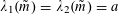
Suppose that the inclusion is symmetric under a rotation by $\unicode[STIX]{x1D70B}$ around at least two of the three coordinate axes. Then the matrices $A^{\text{hom}}$ and $\unicode[STIX]{x1D6E4}(\unicode[STIX]{x1D714})$ are diagonal (see Appendix): $4\unicode[STIX]{x1D70B}^{2}A^{\text{hom}}=\text{diag}(a_{1},a_{2},a_{3}),$ $\unicode[STIX]{x1D6E4}(\unicode[STIX]{x1D714})=\text{diag}(\unicode[STIX]{x1D6FD}_{1}(\unicode[STIX]{x1D714}),\unicode[STIX]{x1D6FD}_{2}(\unicode[STIX]{x1D714}),\unicode[STIX]{x1D6FD}_{3}(\unicode[STIX]{x1D714}))$ . Here $a_{i}$ , $i=1,2,3,$ are positive constants and $\unicode[STIX]{x1D6FD}_{i}$ , $i=1,2,3,$ are real-valued scalar functions. Notice that, since $|\tilde{m}|=1$ , the eigenvalues $\unicode[STIX]{x1D706}_{1,2}(\tilde{m})$ of ${\mathcal{M}}(\tilde{m})$ are the solutions to the quadratic equation

(3.15) $$\begin{eqnarray}\displaystyle & & \displaystyle \unicode[STIX]{x1D706}^{2}-\unicode[STIX]{x1D706}\{(a_{2}+a_{3})\tilde{m}_{1}^{2}+(a_{1}+a_{3})\tilde{m}_{2}^{2}+(a_{1}+a_{2})\tilde{m}_{3}^{2}\}\nonumber\\ \displaystyle & & \displaystyle \quad +\,(a_{1}a_{2}\tilde{m}_{3}^{2}+a_{2}a_{3}\tilde{m}_{1}^{2}+a_{1}a_{3}\tilde{m}_{2}^{2})=0.\end{eqnarray}$$

We will now solve the eigenvalue problem (3.12), equivalently (3.14), for particular examples of such inclusions.

3.3.1 Isotropic propagation (no “weak” band gaps)

If the inclusion $Q_{0}$ is symmetric by a $\unicode[STIX]{x1D70B}/2$ -rotation around at least two of the three axes, say $x_{1}$ and $x_{2},$ then $a=a_{1}=a_{2}=a_{3}$ and $\unicode[STIX]{x1D6FD}(\unicode[STIX]{x1D714})=\unicode[STIX]{x1D6FD}_{1}(\unicode[STIX]{x1D714})=\unicode[STIX]{x1D6FD}_{2}(\unicode[STIX]{x1D714})=\unicode[STIX]{x1D6FD}_{3}(\unicode[STIX]{x1D714})$ . Equation (3.15) takes the form $(\unicode[STIX]{x1D706}-a)^{2}=0,$ and therefore $\unicode[STIX]{x1D706}_{1}(\tilde{m})=\unicode[STIX]{x1D706}_{2}(\tilde{m})=a$ is an eigenvalue of multiplicity two of ${\mathcal{M}}(\tilde{m}),$ with orthonormal eigenvectors given by

(3.16) $$\begin{eqnarray}\tilde{e}_{1}(\tilde{m})=e_{2},\qquad \tilde{e}_{2}(\tilde{m})=e_{3}\quad \text{if }|\tilde{m}_{1}|=1,\end{eqnarray}$$

and

(3.17)

As before, the $e_{j}$ , $j=1,2,3,$ are the Euclidean basis vectors. The system (3.14) takes the form

$$\begin{eqnarray}a|m|^{2}\tilde{u} (\tilde{m})=\unicode[STIX]{x1D6FD}(\unicode[STIX]{x1D714})\tilde{u} (\tilde{m}),\qquad \unicode[STIX]{x1D6FC}(\tilde{m})\unicode[STIX]{x1D6FD}(\unicode[STIX]{x1D714})=0.\end{eqnarray}$$

Notice that if $\unicode[STIX]{x1D714}$ is a zero of $\unicode[STIX]{x1D6FD}$ then necessarily $\tilde{u} (\tilde{m})$ is the zero vector. For such values of $\unicode[STIX]{x1D714},$ the above system is satisfied for any $\unicode[STIX]{x1D6FC}(\tilde{m}),$ that is, the non-trivial eigenvectors to (3.12) are parallel to $\tilde{m}$ . On the other hand, if $\unicode[STIX]{x1D6FD}(\unicode[STIX]{x1D714})\neq 0$ , then $\unicode[STIX]{x1D6FC}(\tilde{m})=0$ and $\unicode[STIX]{x1D714}$ is an eigenvalue of (3.12) if and only if it solves the equation $\unicode[STIX]{x1D6FD}(\unicode[STIX]{x1D714})=a|m|^{2}.$ In this case $\tilde{u} (\tilde{m})$ is an arbitrary element of $\mathbb{R}^{2}$ and $\hat{u} (m)=C(\tilde{m})^{\top }\tilde{u} (\tilde{m})$ is an arbitrary vector of the (two-dimensional) eigenspace spanned by the vectors $\tilde{e}_{1}(\tilde{m})$ and $\tilde{e}_{2}(\tilde{m}).$ Finally, there are no non-trivial solutions $\hat{u}$ when $\unicode[STIX]{x1D6FD}(\unicode[STIX]{x1D714})<0.$

3.3.2 Directional propagation (existence of “weak” band gaps)

If the inclusion $Q_{0}$ is symmetric by a $\unicode[STIX]{x1D70B}/2$ -rotation around one of the three coordinate axis, say $x_{1},$ and by a $\unicode[STIX]{x1D70B}$ -rotation around another axis, say $x_{2},$ one has $a=a_{1}$ , $b=a_{2}=a_{3}$ and $\unicode[STIX]{x1D6FD}_{2}(\unicode[STIX]{x1D714})=\unicode[STIX]{x1D6FD}_{3}(\unicode[STIX]{x1D714})$ . Here, recalling $|\tilde{m}|=1$ , (3.15) takes the form

$$\begin{eqnarray}(\unicode[STIX]{x1D706}-b)(\unicode[STIX]{x1D706}-a(1-\tilde{m}_{1}^{2})-b\tilde{m}_{1}^{2})=0,\end{eqnarray}$$

whence $\unicode[STIX]{x1D706}_{1}(\tilde{m})=a(1-\tilde{m}_{1}^{2})+b\tilde{m}_{1}^{2}$ , $\unicode[STIX]{x1D706}_{2}(\tilde{m})=b$ . There are now two separate cases to consider.

Case 1. Assume that $|\tilde{m}_{1}|=1$ , that is, the vector $\tilde{m}$ is parallel to the axis of higher symmetry. Here, ${\mathcal{M}}(\tilde{m})=\text{diag}(0,b,b)$ and $b$ is an eigenvalue of multiplicity two with the eigenspace spanned by the vectors (3.16). The system (3.14) takes the form

$$\begin{eqnarray}bm_{1}^{2}\tilde{u} (\tilde{m})=\unicode[STIX]{x1D6FD}_{2}(\unicode[STIX]{x1D714})\tilde{u} (\tilde{m}),\qquad \unicode[STIX]{x1D6FC}(\tilde{m})\unicode[STIX]{x1D6FD}_{1}(\unicode[STIX]{x1D714})=0.\end{eqnarray}$$

Here, if $\unicode[STIX]{x1D6FD}_{2}(\unicode[STIX]{x1D714})<0,$ then necessarily $\tilde{u} (\tilde{m})=0$ and non-trivial solutions $\hat{u} (m)=\unicode[STIX]{x1D6FC}(\tilde{m})\tilde{m}$ exist if and only if $\unicode[STIX]{x1D6FD}_{1}(\unicode[STIX]{x1D714})=0.$ On the other hand, if $\unicode[STIX]{x1D6FD}_{1}(\unicode[STIX]{x1D714})<0,$ then necessarily $\unicode[STIX]{x1D6FC}(\tilde{m})=0$ and non-trivial solutions $\hat{u} (m)=C(\tilde{m})^{\top }\tilde{u} (\tilde{m})$ exist if and only if $\unicode[STIX]{x1D6FD}_{2}(\unicode[STIX]{x1D714})>0.$ The first situation only occurs at a discrete set of values  $\unicode[STIX]{x1D714},$ while, unlike in the isotropic case, the second situation can give rise to intervals each of which contains a sequence of admissible $\unicode[STIX]{x1D714},$ obtained from the condition $\sqrt{\unicode[STIX]{x1D6FD}_{2}(\unicode[STIX]{x1D714})/b}\in \mathbb{N},$ with a reduced number of eigenmodes. In the case of the full-space problem these intervals form part of the continuous spectrum of the problem with a reduced number of propagating modes (“weak band gaps”; cf. [Reference Smyshlyaev7, Reference Zhikov and Pastukhova9, Reference Zhikov and Pastukhova10]).

Case 2. Assume $|\tilde{m}_{1}|<1,$ that is, the vector $\tilde{m}$ is not parallel to the axis of higher symmetry. In this case the eigenvectors corresponding to $\unicode[STIX]{x1D706}_{1}(\tilde{m}),$ $\unicode[STIX]{x1D706}_{2}(\tilde{m})$ are given by $\tilde{e}_{1}(\tilde{m}),$ $\tilde{e}_{2}(\tilde{m})$ in (3.17). By setting

$$\begin{eqnarray}\unicode[STIX]{x1D6E4}(\unicode[STIX]{x1D714})=\text{diag}(\unicode[STIX]{x1D6FD}_{1}(\unicode[STIX]{x1D714})-\unicode[STIX]{x1D6FD}_{2}(\unicode[STIX]{x1D714}),0,0)+\unicode[STIX]{x1D6FD}_{2}(\unicode[STIX]{x1D714})I\end{eqnarray}$$

it is easy to see that the system (3.14) takes the form

(3.18)

If $\tilde{m}_{1}=0$ , that is, the vector $\tilde{m}$ is perpendicular to the direction of higher symmetry, then the system (3.18) fully decouples and reduces to

$$\begin{eqnarray}\displaystyle & \displaystyle |m|^{2}a\tilde{u} _{1}(\tilde{m})=\unicode[STIX]{x1D6FD}_{2}(\unicode[STIX]{x1D714})\tilde{u} _{1}(\tilde{m}),\qquad |m|^{2}b\tilde{u} _{2}(\tilde{m})=\unicode[STIX]{x1D6FD}_{1}(\unicode[STIX]{x1D714})\tilde{u} _{2}(\tilde{m}), & \displaystyle \nonumber\\ \displaystyle & \displaystyle \unicode[STIX]{x1D6FC}(\tilde{m})\unicode[STIX]{x1D6FD}_{2}(\unicode[STIX]{x1D714})=0. & \displaystyle \nonumber\end{eqnarray}$$

Suppose $\unicode[STIX]{x1D6FD}_{1}(\unicode[STIX]{x1D714})$ (respectively, $\unicode[STIX]{x1D6FD}_{2}(\unicode[STIX]{x1D714})$ ) is negative for some $\unicode[STIX]{x1D714}$ . Then the above system implies that $\tilde{u} _{2}(\tilde{m})=0$ (respectively, $\tilde{u} _{1}(\tilde{m})=0$ ). In this case, we see that propagation is restricted solely to the direction of $\tilde{e}_{1}(\tilde{m})$ (respectively, $\tilde{e}_{2}(\tilde{m})$ ), which is orthogonal to the eigenvector(s) corresponding to the negative eigenvalue of $\unicode[STIX]{x1D6E4}(\unicode[STIX]{x1D714})$ . In both situations weak band gaps are present in the similar full-space problem.

Remark 3.1. Recently there have been several works on the analysis of problems with “partial” or “directional” wave propagation in the context of elasticity, where at some frequencies, propagation occurs for some but not for all values of the wave vector: the analysis of the vector problems for thin structures of critical thickness [Reference Zhikov and Pastukhova9], the analysis of high-contrast [Reference Zhikov and Pastukhova10], and partially high-contrast [Reference Smyshlyaev7] periodic elastic composites. To our knowledge, the effect we describe here is the first example of a similar kind for Maxwell equations.

Remark 3.2. When the “size” $T$ of the domain $\mathbb{T}$ increases to infinity (equivalently, for a given macroscopic domain, the parameter by which its size is scaled (see §2) tends to zero), the spectrum of (2.4)–(2.6) converges to a union of intervals (“bands”) separated by intervals of those values $\unicode[STIX]{x1D714}^{2}$ for which the matrix $\unicode[STIX]{x1D6E4}(\unicode[STIX]{x1D714})$ is negative definite (“gaps” or “lacunae”). As above, we say that $\unicode[STIX]{x1D714}^{2}$ belongs to a weak band gap (in the spectrum of (2.4)–(2.6)) if at least one eigenvalue of $\unicode[STIX]{x1D6E4}(\unicode[STIX]{x1D714})$ is positive semidefinite and at least one eigenvalue of $\unicode[STIX]{x1D6E4}(\unicode[STIX]{x1D714})$ is negative.

4 Two-scale asymptotic expansion of the eigenfunctions

Here we give the details of the recurrent procedure for the construction of the series (2.2). We use $|_{+}$ and $|_{-}$ to denote the limit values of the expressions to which these symbols are attached, on the outside and on the inside of the boundary of the inclusion $Q_{0}$ , respectively.

Substituting the expansions (2.2) into (2.1) and equating coefficients on $\unicode[STIX]{x1D702}^{-2},\unicode[STIX]{x1D702}^{-1}$ and $\unicode[STIX]{x1D702}^{0},$ we arrive at the following sets of equations, where $x\in \mathbb{T}$ is a parameter:

(4.1) $$\begin{eqnarray}\displaystyle & \displaystyle \text{curl}_{y}(\unicode[STIX]{x1D716}_{1}^{-1}(y)\,\text{curl}_{y}\,H^{0}(x,y))=0,\quad y\in Q_{1}, & \displaystyle\end{eqnarray}$$

(4.2) $$\begin{eqnarray}\displaystyle & \displaystyle \unicode[STIX]{x1D716}_{1}^{-1}(y)\,\text{curl}_{y}\,H^{0}(x,y)\times n(y)|_{+}=0,\quad y\in \unicode[STIX]{x2202}Q_{0}, & \displaystyle\end{eqnarray}$$

(4.3) $$\begin{eqnarray}\displaystyle & & \displaystyle \text{curl}_{y}(\unicode[STIX]{x1D716}_{1}^{-1}(y)\,\text{curl}_{y}\,H^{1}(x,y))\nonumber\\ \displaystyle & & \displaystyle \quad =-(\text{curl}_{y}\,\unicode[STIX]{x1D716}_{1}^{-1}(y)\,\text{curl}_{x}+\text{curl}_{x}\,\unicode[STIX]{x1D716}_{1}^{-1}(y)\,\text{curl}_{y})H^{0}(x,y),\quad y\in Q_{1},\end{eqnarray}$$

(4.4) $$\begin{eqnarray}\displaystyle & & \displaystyle (\unicode[STIX]{x1D716}_{1}^{-1}(y)\,\text{curl}_{y}\,H^{1}(x,y)\times n(y)+\unicode[STIX]{x1D716}_{1}^{-1}(y)\,\text{curl}_{x}\,H^{0}(x,y)\times n(y))|_{+}=0,\nonumber\\ \displaystyle & & \displaystyle \quad y\in \unicode[STIX]{x2202}Q_{0},\end{eqnarray}$$

(4.5) $$\begin{eqnarray}\displaystyle & & \displaystyle \text{curl}_{y}(\unicode[STIX]{x1D716}_{1}^{-1}(y)\,\text{curl}_{y}\,H^{2}(x,y))\nonumber\\ \displaystyle & & \displaystyle \quad =-(\text{curl}_{y}\,\unicode[STIX]{x1D716}_{1}^{-1}(y)\,\text{curl}_{x}+\text{curl}_{x}\,\unicode[STIX]{x1D716}_{1}^{-1}(y)\,\text{curl}_{y})H^{1}(x,y)\nonumber\\ \displaystyle & & \displaystyle \qquad -\,\text{curl}_{x}\,\unicode[STIX]{x1D716}_{1}^{-1}(y)\,\text{curl}_{x}\,H^{0}(x,y)+\unicode[STIX]{x1D714}^{2}H^{0}(x,y),\quad y\in Q_{1},\end{eqnarray}$$

(4.6) $$\begin{eqnarray}\displaystyle & & \displaystyle (\unicode[STIX]{x1D716}_{1}^{-1}(y)\,\text{curl}_{y}\,H^{2}(x,y)+\unicode[STIX]{x1D716}_{1}^{-1}(y)\,\text{curl}_{x}\,H^{1}(x,y))\times n(y)|_{+}\nonumber\\ \displaystyle & & \displaystyle \quad =\unicode[STIX]{x1D716}_{0}^{-1}(y)\,\text{curl}_{y}\,H^{0}(x,y)\times n(y)|_{-},\quad y\in \unicode[STIX]{x2202}Q_{0},\end{eqnarray}$$

and

(4.7) $$\begin{eqnarray}\displaystyle & \displaystyle \text{curl}_{y}(\unicode[STIX]{x1D716}_{0}^{-1}(y)\,\text{curl}_{y}\,H^{0}(x,y))=\unicode[STIX]{x1D714}^{2}H^{0}(x,y),\quad y\in Q_{0}, & \displaystyle\end{eqnarray}$$

(4.8) $$\begin{eqnarray}\displaystyle & \displaystyle H^{0}(x,y)|_{-}=H^{0}(x,y)|_{+},\quad y\in \unicode[STIX]{x2202}Q_{0}. & \displaystyle\end{eqnarray}$$

Multiplying equation (4.1) by $H^{0}$ , integrating by parts over $Q_{1}$ and using (4.2) shows that $\text{curl}_{y}\,H^{0}(x,y)=0$ , $y\in Q_{1}.$ More precisely, for all $x\in \mathbb{T}$ , we seek $H^{0}(x,\cdot )$ from the space $V$ ; see (2.8). Before proceeding, we recall a characterization of the space $V$ (see [Reference Cherednichenko and Cooper1]) that proves useful in the analysis of the term $H^{0}$ .

Lemma 4.1 (Characterization of $V$ ).

A function $v\in [H_{\#}^{1}(Q)]^{3}$ is an element of the space $V$ if and only if

$$\begin{eqnarray}v(y)=a+\unicode[STIX]{x1D6FB}b(y)+c(y)\quad \text{a.e. }y\in Q,\end{eqnarray}$$

for some $a\in \mathbb{R}^{3}$ , $b\in H_{\#}^{2}(Q)$ , $c\in [H_{0}^{1}(Q_{0})]^{3}$ .

Taking into account, via Lemma 4.1, that the leading-order term $H^{0}$ is of the form

(4.9) $$\begin{eqnarray}H^{0}(x,y)=u(x)+\unicode[STIX]{x1D6FB}_{y}v(x,y)+z(x,y)\end{eqnarray}$$

and substituting (4.9) into equations (4.3)–(4.4), we find that the coefficient $H^{1}$ has the representation $H^{1}(x,y)=N(y)\,\text{curl}\,u(x)+\widetilde{H}^{1}(x,y),$ up to the addition of an element of $V$ . Here the term $\widetilde{H}^{1}(x,y)$ satisfies

(4.10) $$\begin{eqnarray}\displaystyle \text{curl}_{y}(\unicode[STIX]{x1D716}_{1}^{-1}(y)\,(\text{curl}_{y}\,\widetilde{H}^{1}(x,y)+\text{curl}_{x}\unicode[STIX]{x1D6FB}_{y}v(x,y))) & = & \displaystyle 0,\quad y\in Q_{1},\end{eqnarray}$$

(4.11) $$\begin{eqnarray}\displaystyle \unicode[STIX]{x1D716}_{1}^{-1}(y)(\text{curl}_{y}\,\widetilde{H}^{1}(x,y)+\text{curl}_{x}\unicode[STIX]{x1D6FB}_{y}v(x,y))\times n(y)|_{+} & = & \displaystyle 0,\quad y\in \unicode[STIX]{x2202}Q_{0},\qquad\end{eqnarray}$$

and $N=N(y)$ is a $Q$ -periodic matrix-valued function whose columns $N^{r}=N^{r}(y)$ , $r=1,2,3,$ are solutions to the problems

(4.12) $$\begin{eqnarray}\displaystyle \begin{array}{@{}c@{}}\displaystyle \text{curl}_{}(\unicode[STIX]{x1D716}_{1}^{-1}(y)(\text{curl}_{}\,N^{r}(y)+e^{r}))=0,\quad y\in Q_{1},\\ \displaystyle \unicode[STIX]{x1D716}_{1}^{-1}(y)(\text{curl}_{}\,N^{r}(y)+e^{r})\times n(y)=0,\quad y\in \unicode[STIX]{x2202}Q_{0},\end{array} & & \displaystyle\end{eqnarray}$$

where $e^{r}$ is the $r$ th Euclidean basis vector. It is shown [Reference Cooper4, Reference Kamotski and Smyshlyaev6] that (4.12) admits a unique solution in $V^{\bot },$ the orthogonal complement to $V$ in the space $[H_{\#}^{1}(Q)]^{3}.$

Looking for $H^{1}(x,\cdot )\in [H_{\#}^{1}(Q)]^{3}$ and taking into account the identity $\text{curl}_{x}\unicode[STIX]{x1D6FB}_{y}=-\text{curl}_{y}\unicode[STIX]{x1D6FB}_{x}$ together with (4.10)–(4.11), we infer that for all $x\in \mathbb{T}$ the function $h(x,\cdot ):=\widetilde{H}^{1}(x,\cdot )-\unicode[STIX]{x1D6FB}_{x}v(x,\cdot )$ is a solution in $[H_{\#}^{1}(Q)]^{3}$ to

$$\begin{eqnarray}\displaystyle \begin{array}{@{}c@{}}\displaystyle \text{curl}_{y}(\unicode[STIX]{x1D716}_{1}^{-1}(y)\,\text{curl}_{y}\,h(x,y))=0,\quad y\in Q_{1},\\ \displaystyle \unicode[STIX]{x1D716}_{1}^{-1}(y)\,\text{curl}_{y}\,h(x,y)\times n(y)|_{+}=0,\quad y\in \unicode[STIX]{x2202}Q_{0}.\end{array} & & \displaystyle \nonumber\end{eqnarray}$$

In particular, the function $h$ belongs to the space $V$ . Therefore, one has

(4.13) $$\begin{eqnarray}H^{1}(x,y)=N(y)\,\text{curl}_{x}\,u(x)+\unicode[STIX]{x1D6FB}_{x}v(x,y),\end{eqnarray}$$

up to the addition of an element of $V$ . (As we discuss in Remark 5.1 below, one can specify the divergence $\text{div}_{y}H^{1}(x,y).$ This, along with the condition that the $y$ -average of $H^{1}$ vanishes, defines this additional element of $V$ in a unique way.)

Further, multiplying equation (4.5) by an arbitrary test function $\unicode[STIX]{x1D719}\in V$ and integrating over $Q_{1}$ yields

(4.14) $$\begin{eqnarray}\displaystyle & & \displaystyle \int _{Q_{1}}\text{curl}_{y}(\unicode[STIX]{x1D716}_{1}^{-1}(y)\,\text{curl}_{y}\,H^{2}(x,y))\cdot \unicode[STIX]{x1D719}(y)\,dy\nonumber\\ \displaystyle & & \displaystyle \quad =\int _{Q_{1}}\unicode[STIX]{x1D714}^{2}H^{0}(x,y)\cdot \unicode[STIX]{x1D719}(y)\,dy-\int _{Q_{1}}\text{curl}_{y}(\unicode[STIX]{x1D716}_{1}^{-1}(y)\,\text{curl}_{x}\,H^{1}(x,y))\cdot \unicode[STIX]{x1D719}(y)\,dy\nonumber\\ \displaystyle & & \displaystyle \qquad -\,\biggl(\int _{Q_{1}}\text{curl}_{x}(\unicode[STIX]{x1D716}_{1}^{-1}(y)\,\text{curl}_{x}\,H^{0}(x,y))\cdot \unicode[STIX]{x1D719}(y)\nonumber\\ \displaystyle & & \displaystyle \qquad +\,\text{curl}_{x}(\unicode[STIX]{x1D716}_{1}^{-1}(y)\,\text{curl}_{y}\,H^{1}(x,y))\cdot \unicode[STIX]{x1D719}(y)\,dy\biggr).\end{eqnarray}$$

We integrate in the left-hand side of (4.14) by parts to determine that

(4.15) $$\begin{eqnarray}\displaystyle & & \displaystyle \int _{Q_{1}}\text{curl}_{y}(\unicode[STIX]{x1D716}_{1}^{-1}(y)\,\text{curl}_{y}\,H^{2}(x,y))\cdot \unicode[STIX]{x1D719}(y)\,dy\nonumber\\ \displaystyle & & \displaystyle \quad =\int _{\unicode[STIX]{x2202}Q_{0}}\unicode[STIX]{x1D716}_{1}^{-1}(y)(\text{curl}_{y}\,H^{2}(x,y)\times n(y)|_{+})\cdot \unicode[STIX]{x1D719}(y)\,dS(y).\end{eqnarray}$$

Now we perform integration by parts on the individual terms on the right-hand side of (4.14).

(4.16) $$\begin{eqnarray}\displaystyle & & \displaystyle -\int _{Q_{1}}\text{curl}_{y}(\unicode[STIX]{x1D716}_{1}^{-1}(y)\,\text{curl}_{x}\,H^{1}(x,y))\unicode[STIX]{x1D719}(y)\,dy\nonumber\\ \displaystyle & & \displaystyle \qquad =-\int _{\unicode[STIX]{x2202}Q_{0}}(\unicode[STIX]{x1D716}_{1}^{-1}(y)\,\text{curl}_{x}\,H^{1}(x,y)\times n(y)|_{+})\cdot \unicode[STIX]{x1D719}(y)\,dS(y)\nonumber\\ \displaystyle & & \displaystyle \,\quad \overset{\text{by (4.6)}}{=}\int _{\unicode[STIX]{x2202}Q_{0}}\{(\unicode[STIX]{x1D716}_{1}^{-1}(y)\,\text{curl}_{y}\,H^{2}(x,y)\times n(y)|_{+})\cdot \unicode[STIX]{x1D719}(y)\nonumber\\ \displaystyle & & \displaystyle \quad \qquad -\,(\unicode[STIX]{x1D716}_{0}^{-1}(y)\,\text{curl}_{y}\,H^{0}(x,y)\times n(y)|_{-})\cdot \unicode[STIX]{x1D719}(y)\!\}\,dS(y)\nonumber\\ \displaystyle & & \displaystyle \qquad =\int _{\unicode[STIX]{x2202}Q_{0}}(\unicode[STIX]{x1D716}_{1}^{-1}(y)\,\text{curl}_{y}\,H^{2}(x,y)\times n(y)|_{+})\cdot \unicode[STIX]{x1D719}(y)\,dS(y)\nonumber\\ \displaystyle & & \displaystyle \quad \qquad +\,\int _{Q_{0}}\text{curl}_{y}(\unicode[STIX]{x1D716}_{0}^{-1}(y)\,\text{curl}_{y}\,H^{0}(x,y))\cdot \unicode[STIX]{x1D719}(y)\,dy\nonumber\\ \displaystyle & & \displaystyle \quad \qquad -\,\int _{Q_{0}}\unicode[STIX]{x1D716}_{0}^{-1}(y)\,\text{curl}_{y}\,H^{0}(x,y)\cdot \text{curl}_{y}\,\unicode[STIX]{x1D719}(y)\,dy\nonumber\\ \displaystyle & & \displaystyle \,\quad \overset{\text{by (4.7)}}{=}\int _{\unicode[STIX]{x2202}Q_{0}}(\unicode[STIX]{x1D716}_{1}^{-1}(y)\,\text{curl}_{y}\,H^{2}(x,y)\times n(y)|_{+})\cdot \unicode[STIX]{x1D719}(y)\,dS(y)\nonumber\\ \displaystyle & & \displaystyle \quad \qquad +\,\int _{Q_{0}}\unicode[STIX]{x1D714}^{2}H^{0}(x,y)\cdot \unicode[STIX]{x1D719}(y)\,dy\nonumber\\ \displaystyle & & \displaystyle \quad \qquad -\,\int _{Q_{0}}\unicode[STIX]{x1D716}_{0}^{-1}(y)\,\text{curl}_{y}\,H^{0}(x,y)\cdot \text{curl}_{y}\,\unicode[STIX]{x1D719}(y)\,dy.\end{eqnarray}$$

Taking into account the representations (4.9) and (4.13), we find that

(4.17) $$\begin{eqnarray}\displaystyle & & \displaystyle \int _{Q_{1}}\{\!\text{curl}_{x}(\unicode[STIX]{x1D716}_{1}^{-1}(y)\,\text{curl}_{x}\,H^{0}(x,y))\cdot \unicode[STIX]{x1D719}(y)\nonumber\\ \displaystyle & & \displaystyle \qquad +\,\text{curl}_{x}(\unicode[STIX]{x1D716}_{1}^{-1}(y)\,\text{curl}_{y}\,H^{1}(x,y))\cdot \unicode[STIX]{x1D719}(y)\!\}\,dy\nonumber\\ \displaystyle & & \displaystyle \quad =\int _{Q_{1}}\text{curl}_{x}\!\{\!\unicode[STIX]{x1D716}_{1}^{-1}(y)(\,(I+\text{curl}\,N(y))\,\text{curl}_{x}\,u(x)\nonumber\\ \displaystyle & & \displaystyle \qquad +\,\text{curl}_{x}\unicode[STIX]{x1D6FB}_{y}v(x,y)+\text{curl}_{y}\unicode[STIX]{x1D6FB}_{x}v(x,y))\!\}\cdot \,\unicode[STIX]{x1D719}(y)\,dy\nonumber\\ \displaystyle & & \displaystyle \quad =\int _{Q_{1}}\text{curl}_{x}\{\unicode[STIX]{x1D716}_{1}^{-1}(y)(I+\text{curl}\,N(y))\,\text{curl}_{x}\,u(x)\}\cdot \unicode[STIX]{x1D719}(y)\,dy,\end{eqnarray}$$

where we again make use of the identity $\text{curl}_{x}\unicode[STIX]{x1D6FB}_{y}=-\text{curl}_{y}\unicode[STIX]{x1D6FB}_{x}.$ Finally, equations (4.14)–(4.17) imply

(4.18) $$\begin{eqnarray}\displaystyle & & \displaystyle \int _{Q_{1}}\text{curl}_{x}\{\unicode[STIX]{x1D716}_{1}^{-1}(y)(I+\text{curl}\,N(y))\,\text{curl}_{x}\,u(x)\}\cdot \unicode[STIX]{x1D719}(y)\,dy\nonumber\\ \displaystyle & & \displaystyle \qquad +\,\int _{Q_{0}}\unicode[STIX]{x1D716}_{0}^{-1}(y)\,\text{curl}_{y}H^{0}(x,y)\cdot \text{curl}_{y}\,\unicode[STIX]{x1D719}(y)\,dy\nonumber\\ \displaystyle & & \displaystyle \quad =\int _{Q}\unicode[STIX]{x1D714}^{2}H^{0}(x,y)\cdot \unicode[STIX]{x1D719}(y)\,dy\quad \text{for all }\unicode[STIX]{x1D719}\in V.\end{eqnarray}$$

In what follows we derive the system (2.4)–(2.6) by considering different choices of the test function $\unicode[STIX]{x1D719}$ in the identity (4.18).

Step 1. Choosing test functions $\unicode[STIX]{x1D719}\in [C_{0}^{\infty }(Q_{0})]^{3}$ in (4.18), we find that

$$\begin{eqnarray}\text{curl}_{y}(\unicode[STIX]{x1D716}_{0}^{-1}(y)\,\text{curl}_{y}\,H^{0}(x,y))=\unicode[STIX]{x1D714}^{2}H^{0}(x,y),\quad y\in Q_{0}.\end{eqnarray}$$

Using the representation (4.9) and the identity $\text{curl}_{y}\unicode[STIX]{x1D6FB}_{y}=0$ , we arrive at (2.6).

Step 2. Choosing $\unicode[STIX]{x1D719}=\unicode[STIX]{x1D6FB}_{y}\unicode[STIX]{x1D713}$ in (4.18), performing integration by parts, using the identity $\text{div}_{y}\,\text{curl}_{x}=-\text{div}_{x}\,\text{curl}_{y}$ and recalling (4.12) gives

$$\begin{eqnarray}\displaystyle & & \displaystyle \int _{Q}\unicode[STIX]{x1D714}^{2}H^{0}(x,y)\cdot \unicode[STIX]{x1D6FB}_{y}\unicode[STIX]{x1D713}\,dy\nonumber\\ \displaystyle & & \displaystyle \quad =\int _{Q_{1}}\text{curl}_{x}\{\unicode[STIX]{x1D716}_{1}^{-1}(y)(I+\text{curl}\,N(y))\,\text{curl}_{x}\,u(x)\}\cdot \unicode[STIX]{x1D6FB}_{y}\unicode[STIX]{x1D713}(y)\,dy\nonumber\\ \displaystyle & & \displaystyle \quad =-\int _{Q_{1}}\text{div}_{y}\,\text{curl}_{x}\{\unicode[STIX]{x1D716}_{1}^{-1}(y)(I+\text{curl}\,N(y))\,\text{curl}_{x}\,u(x)\}\cdot \unicode[STIX]{x1D713}(y)\,dy\nonumber\\ \displaystyle & & \displaystyle \quad =\int _{Q_{1}}\text{div}_{x}\,\text{curl}_{y}\{\unicode[STIX]{x1D716}_{1}^{-1}(y)(I+\text{curl}\,N(y))\,\text{curl}_{x}\,u(x)\}\cdot \unicode[STIX]{x1D713}(y)\,dy=0.\nonumber\end{eqnarray}$$

Therefore, we deduce that

(4.19) $$\begin{eqnarray}\text{div}_{y}H^{0}(x,y)=0,\quad y\in Q,\end{eqnarray}$$

and, taking into account (4.9), we obtain the equation (2.5).

Step 3. Choosing $\unicode[STIX]{x1D719}(y)\equiv 1$ in the identity (4.18), we find, using the representation (4.9) once more, that (2.4) holds, where the matrix $A^{\text{hom}}$ emerges as the result of integrating the expression $\unicode[STIX]{x1D716}_{1}^{-1}(y)(\text{curl}\,N(y)+I)$ with respect to $y\in Q_{1}.$

In the next section we use the above formal construction of the series (2.2) to justify the two claims of Theorem 2.1.

5 Proof of Theorem 2.1

For each $\unicode[STIX]{x1D702}>0,$ denote by ${\mathcal{A}}_{\unicode[STIX]{x1D702}}$ the operator in the spaceFootnote ⁵ $L_{\#\text{sol}}^{2}(\mathbb{T})$ defined in a standard way by the bilinear form (cf. (2.1))

$$\begin{eqnarray}\int _{\mathbb{T}}\unicode[STIX]{x1D700}_{\unicode[STIX]{x1D702}}^{-1}\biggl(\frac{\cdot }{\unicode[STIX]{x1D702}}\biggr)\text{curl}\,u\cdot \text{curl}\,v,\quad u,v\in [H_{\#}^{1}(\mathbb{T})]^{3}\cap L_{\#\text{sol}}^{2}(\mathbb{T})=:{\mathcal{H}}.\end{eqnarray}$$

For fixed $\unicode[STIX]{x1D714}$ in the spectrum of (2.4)–(2.6), let $H^{0}$ be a corresponding eigenfunction. Consider the (unique) solution $\widetilde{H}^{\unicode[STIX]{x1D702}}\in {\mathcal{H}}$ to the problem

(5.1) $$\begin{eqnarray}({\mathcal{A}}_{\unicode[STIX]{x1D702}}+I)\widetilde{H}^{\unicode[STIX]{x1D702}}=(\unicode[STIX]{x1D714}^{2}+1)H^{0}\biggl(\cdot ,\frac{\cdot }{\unicode[STIX]{x1D702}}\biggr).\end{eqnarray}$$

Denote also

$$\begin{eqnarray}\mathfrak{b}_{\unicode[STIX]{x1D702}}(u,v):=\int _{\mathbb{T}}\unicode[STIX]{x1D700}_{\unicode[STIX]{x1D702}}^{-1}\biggl(\frac{\cdot }{\unicode[STIX]{x1D702}}\biggr)\text{curl}\,u\cdot \text{curl}\,v+\int _{\mathbb{T}}u\cdot v,\quad u,v\in [H_{\#}^{1}(\mathbb{T})]^{3},\end{eqnarray}$$

and (cf. (2.2))

(5.2) $$\begin{eqnarray}H^{(2)}(\cdot ,\unicode[STIX]{x1D702}):=H^{0}\biggl(\cdot ,\frac{\cdot }{\unicode[STIX]{x1D702}}\biggr)+\unicode[STIX]{x1D702}H^{1}\biggl(\cdot ,\frac{\cdot }{\unicode[STIX]{x1D702}}\biggr)+\unicode[STIX]{x1D702}^{2}H^{2}\biggl(\cdot ,\frac{\cdot }{\unicode[STIX]{x1D702}}\biggr),\end{eqnarray}$$

where $H^{j}$ , $j=1,2,$ are solutions of the system of recurrence relations described in §4. The existence of solutions $H^{1}$ , $H^{2}$ is guaranteed by a result established in [Reference Cherednichenko and Cooper1, Lemma 3.4]. As these solutions are unique up to the addition of an element from $V$ , we shall choose them as in Remark 5.1.

Proposition 5.1. There exists a constant $\widehat{C}>0$ such that the estimate

(5.3)

holds for all $\unicode[STIX]{x1D711}\in [H_{\#}^{1}(\mathbb{T})]^{3}.$

Proof. Using the definition of the function $\widetilde{H}^{\unicode[STIX]{x1D702}}$ and the recurrence relations (4.1)–(4.8) yields

(5.4) $$\begin{eqnarray}\displaystyle & & \displaystyle \mathfrak{b}_{\unicode[STIX]{x1D702}}(\widetilde{H}^{\unicode[STIX]{x1D702}}-H^{(2)}(\cdot ,\unicode[STIX]{x1D702}),\unicode[STIX]{x1D711})\nonumber\\ \displaystyle & & \displaystyle \quad =\int _{\mathbb{T}}\unicode[STIX]{x1D700}_{\unicode[STIX]{x1D702}}^{-1}\biggl(\frac{\cdot }{\unicode[STIX]{x1D702}}\biggr)\text{curl}\,\widetilde{H}^{\unicode[STIX]{x1D702}}\cdot \text{curl}\,\unicode[STIX]{x1D711}+\int _{\mathbb{T}}\widetilde{H}^{\unicode[STIX]{x1D702}}\cdot \unicode[STIX]{x1D711}\nonumber\\ \displaystyle & & \displaystyle \qquad -\,\int _{\mathbb{T}}\unicode[STIX]{x1D700}_{\unicode[STIX]{x1D702}}^{-1}\biggl(\frac{\cdot }{\unicode[STIX]{x1D702}}\biggr)\,\text{curl}\biggl(H^{0}\biggl(\cdot ,\frac{\cdot }{\unicode[STIX]{x1D702}}\biggr)+\unicode[STIX]{x1D702}H^{1}\biggl(\cdot ,\frac{\cdot }{\unicode[STIX]{x1D702}}\biggr)+\unicode[STIX]{x1D702}^{2}H^{2}\biggl(\cdot ,\frac{\cdot }{\unicode[STIX]{x1D702}}\biggr)\biggr)\cdot \text{curl}\,\unicode[STIX]{x1D711}\nonumber\\ \displaystyle & & \displaystyle \qquad -\,\int _{\mathbb{T}}\biggl(H^{0}\biggl(\cdot ,\frac{\cdot }{\unicode[STIX]{x1D702}}\biggr)+\unicode[STIX]{x1D702}H^{1}\biggl(\cdot ,\frac{\cdot }{\unicode[STIX]{x1D702}}\biggr)+\unicode[STIX]{x1D702}^{2}H^{2}\biggl(\cdot ,\frac{\cdot }{\unicode[STIX]{x1D702}}\biggr)\biggr)\cdot \unicode[STIX]{x1D711}\nonumber\\ \displaystyle & & \displaystyle \quad =\int _{\mathbb{T}}F^{1}(\cdot ,\unicode[STIX]{x1D702})\cdot \unicode[STIX]{x1D711}+\int _{\mathbb{T}}F^{2}(\cdot ,\unicode[STIX]{x1D702})\cdot \unicode[STIX]{x1D702}\,\text{curl}_{}\unicode[STIX]{x1D711}.\end{eqnarray}$$

Here, $F^{1},F^{2}$ are elements of $L^{2}(\mathbb{T})$ defined for a.e. $x\in \mathbb{T}$ by

(5.5) $$\begin{eqnarray}\displaystyle F^{1}(x,\unicode[STIX]{x1D702}) & = & \displaystyle -\unicode[STIX]{x1D702}(\unicode[STIX]{x1D712}_{0}(y)\,\text{curl}_{x}(\unicode[STIX]{x1D716}_{0}^{-1}(y)\,\text{curl}_{y}\,H^{0}(x,y))\nonumber\\ \displaystyle & & \displaystyle +\,\unicode[STIX]{x1D712}_{1}(y)\{\!\text{curl}_{x}(\unicode[STIX]{x1D716}_{1}^{-1}(y)\,\text{curl}_{x}\,H^{1}(x,y))\nonumber\\ \displaystyle & & \displaystyle +\,\text{curl}_{x}(\unicode[STIX]{x1D716}_{1}^{-1}(y)\,\text{curl}_{y}\,H^{2}(x,y))\!\}+H^{1}(x,y)+\unicode[STIX]{x1D702}H^{2}(x,y))\!|_{y=x/\unicode[STIX]{x1D702}},\nonumber\\ \displaystyle F^{2}(x,\unicode[STIX]{x1D702}) & = & \displaystyle -\unicode[STIX]{x1D702}(\unicode[STIX]{x1D712}_{0}(y)\unicode[STIX]{x1D716}_{0}^{-1}(y)\{\!\text{curl}_{x}\,H^{0}(x,y)\nonumber\\ \displaystyle & & \displaystyle +\,\text{curl}_{y}\,H^{1}(x,y)+\unicode[STIX]{x1D702}\,\text{curl}_{x}\,H^{1}(x,y)\nonumber\\ \displaystyle & & \displaystyle +\,\unicode[STIX]{x1D702}\,\text{curl}_{y}\,H^{2}(x,y)+\unicode[STIX]{x1D702}^{2}\,\text{curl}_{x}\,H^{2}(x,y)\!\}\nonumber\\ \displaystyle & & \displaystyle +\,\unicode[STIX]{x1D712}_{1}(y)\unicode[STIX]{x1D716}_{1}^{-1}(y)\,\text{curl}_{x}\,H^{2}(x,y))\!|_{y=x/\unicode[STIX]{x1D702}}.\end{eqnarray}$$

Notice that the functions $H^{0}=H^{0}(x,y),H^{1}=H^{1}(x,y),H^{2}=H^{2}(x,y)$ all belong to the space $C_{\#}^{\infty }(\mathbb{T},H_{\#}^{1}(Q))$ . Indeed, this is seen to be true for $H^{0}$ by Proposition 3.1; in the case of $\unicode[STIX]{x1D714}=\unicode[STIX]{x1D6FC}^{k}$ we choose $w\in C_{\#}^{\infty }(\mathbb{T})$ . The assertions for $H^{1}$ and $H^{2}$ now follow from formula (4.13) for the corrector $H^{1}(x,y),$ and the boundary-value problem (4.5)–(4.6) for the function $H^{2}(x,y).$ It then follows from (5.5) (see, for example, [Reference Cherednichenko and Smyshlyaev3, p. 1353]) that $\Vert F^{1}(\cdot ,\unicode[STIX]{x1D702})\Vert _{L^{2}(\mathbb{T})}\leqslant C\unicode[STIX]{x1D702}$ , $\Vert F^{2}(\cdot ,\unicode[STIX]{x1D702})\Vert _{L^{2}(\mathbb{T})}\leqslant C\unicode[STIX]{x1D702}$ , and by applying the Hölder inequality to (5.4) we deduce that

$$\begin{eqnarray}|\mathfrak{b}_{\unicode[STIX]{x1D702}}(\widetilde{H}^{\unicode[STIX]{x1D702}}-H^{(2)}(\cdot ,\unicode[STIX]{x1D702}),\unicode[STIX]{x1D711})|\leqslant C\unicode[STIX]{x1D702}\biggl(\int _{\mathbb{ T}}|\unicode[STIX]{x1D711}|^{2}+\int _{\mathbb{ T}}|\unicode[STIX]{x1D702}\,\text{curl}\,\unicode[STIX]{x1D711}|^{2}\biggr)^{1/2},\end{eqnarray}$$

as required.◻

The above proposition implies the following statement.

Theorem 5.1. There exists a constant $C$ such that the estimate

$$\begin{eqnarray}\Vert \widetilde{H}^{\unicode[STIX]{x1D702}}-H^{0}(\cdot ,\cdot /\unicode[STIX]{x1D702})\Vert _{L^{2}(\mathbb{T})}\leqslant C\unicode[STIX]{x1D702}\end{eqnarray}$$

holds for all $\unicode[STIX]{x1D702}.$

Proof. Setting $\unicode[STIX]{x1D711}=\widetilde{H}^{\unicode[STIX]{x1D702}}-H^{(2)}(\cdot ,\unicode[STIX]{x1D702})$ in the estimate (5.3) yields

$$\begin{eqnarray}\widehat{C}^{2}\unicode[STIX]{x1D702}^{2}\geqslant \mathfrak{b}_{\unicode[STIX]{x1D702}}(\widetilde{H}^{\unicode[STIX]{x1D702}}-H^{(2)}(\cdot ,\unicode[STIX]{x1D702}),\widetilde{H}^{\unicode[STIX]{x1D702}}-H^{(2)}(\cdot ,\unicode[STIX]{x1D702}))\geqslant \Vert \widetilde{H}^{\unicode[STIX]{x1D702}}-H^{(2)}(\cdot ,\unicode[STIX]{x1D702})\Vert _{L^{2}(\mathbb{T})}^{2}.\end{eqnarray}$$

The claim of the theorem now follows by noting that in view of (5.2), we have

$$\begin{eqnarray}\Vert H^{(2)}(\cdot ,\unicode[STIX]{x1D702})-H^{0}(\cdot ,\cdot /\unicode[STIX]{x1D702})\Vert _{L^{2}(\mathbb{T})}\leqslant \widetilde{C}\unicode[STIX]{x1D702}\end{eqnarray}$$

for some $\widetilde{C}>0,$ and hence

$$\begin{eqnarray}\displaystyle \Vert \widetilde{H}^{\unicode[STIX]{x1D702}}-H^{0}(\cdot ,\cdot /\unicode[STIX]{x1D702})\Vert _{L^{2}(\mathbb{T})} & {\leqslant} & \displaystyle \Vert \widetilde{H}^{\unicode[STIX]{x1D702}}-H^{(2)}(\cdot ,\unicode[STIX]{x1D702})\Vert _{L^{2}(\mathbb{T})}\nonumber\\ \displaystyle & & \displaystyle +\,\Vert H^{(2)}(\cdot ,\unicode[STIX]{x1D702})-H^{0}(\cdot ,\cdot /\unicode[STIX]{x1D702})\Vert _{L^{2}(\mathbb{T})}\leqslant (\widehat{C}+\widetilde{C})\unicode[STIX]{x1D702},\nonumber\end{eqnarray}$$

as required. ◻

The claims of Theorem 2.1 now follow from the estimate

(5.6) $$\begin{eqnarray}\displaystyle & & \displaystyle \Vert ((\unicode[STIX]{x1D714}^{2}+1)^{-1}-({\mathcal{A}}_{\unicode[STIX]{x1D702}}+I)^{-1})H^{0}(\cdot ,\cdot /\unicode[STIX]{x1D702})\Vert _{L^{2}(\mathbb{T})}\nonumber\\ \displaystyle & & \displaystyle \quad \leqslant (\unicode[STIX]{x1D714}^{2}+1)^{-1}\Vert H^{0}(\cdot ,\cdot /\unicode[STIX]{x1D702})-\widetilde{H}^{\unicode[STIX]{x1D702}}\Vert _{L^{2}(\mathbb{T})}\leqslant C\unicode[STIX]{x1D702},\end{eqnarray}$$

where we used the definition (5.1) of the function $\widetilde{H}^{\unicode[STIX]{x1D702}}$ and Theorem 5.1. Indeed, from [Reference Vishik and Lyusternik8, p. 109], we infer that the quantities $\text{dist}((\unicode[STIX]{x1D714}^{2}+1)^{-1},\text{Sp}(({\mathcal{A}}_{\unicode[STIX]{x1D702}}+1)^{-1}))$ and $\text{dist}((\unicode[STIX]{x1D714}^{2}+1)^{-1}H^{0}(\cdot ,\cdot /\unicode[STIX]{x1D702}),X_{\unicode[STIX]{x1D702}})$ are controlled above by the right-hand side of (5.6), which completes the proof of Theorem 2.1.

Remark 5.1. Note that $H^{(2)}$ is not solenoidal in general, but can be defined in such a way that it is “close” to a solenoidal field, thanks to equation (4.19) (equivalently, (2.5)) and the special choice of the function $H^{1}$ so that

$$\begin{eqnarray}\text{div}_{x}H^{0}(x,y)+\text{div}_{y}H^{1}(x,y)=0\quad \text{a.e. }(x,y)\in \mathbb{T}\times Q.\end{eqnarray}$$

The function $H^{(2)}$ thus defined is $\unicode[STIX]{x1D702}$ -close to the eigenspace $X_{\unicode[STIX]{x1D702}}$ in the norm of $[H_{\#}^{1}(Q)]^{3}$ .