


1. Introduction
Hypersaline water bodies such as the Dead Sea, soda lakes or industrial salt ponds frequently exist in a state where they are fully saturated with salt. If such a saturated brine layer is cooled from above, its vertical density profile is modified via two separate mechanisms. On one hand, the lower temperature will raise the fluid density near the surface. The thickness of this cold fluid layer will grow diffusively until a critical value of a suitably defined Rayleigh number is reached for thermal convection to begin (Foster Reference Foster1965; Horsch & Stefan Reference Horsch and Stefan1988; Horsch, Stefan & Gavali Reference Horsch, Stefan and Gavali1994; Bednarz, Lei & Patterson Reference Bednarz, Lei and Patterson2009). Concurrently, the lower temperature reduces the solubility of salt in the brine, so that dense halite crystals precipitate and subsequently settle under gravity, thereby giving rise to a sedimenting particle front that can develop its own instabilities (Burns & Meiburg Reference Burns and Meiburg2012, Reference Burns and Meiburg2015; Sutherland, Barrett & Gingras Reference Sutherland, Barrett and Gingras2015). Hence, cooling the brine triggers the formation of both a temperature density front as well as a density front of settling crystals. The present study investigates the evolution and interaction of these density fronts by means of numerical simulations to provide an understanding of the mechanisms governing the sedimentation of the crystals. This, in turn, is important for predicting the evolution of the salt deposits in the Dead Sea in time and space (Sirota, Arnon & Lensky Reference Sirota, Arnon and Lensky2016; Sirota, Enzel & Lensky Reference Sirota, Enzel and Lensky2017).
2. Problem set-up and governing equations
Within the current investigation, we focus on the early, predominantly two-dimensional stages of the frontal evolution, so that we limit ourselves to two-dimensional direct numerical simulations in a rectangular region of height  $H$ and width $W$. Initially, the domain contains saturated brine of constant temperature $T_0$, salinity $S_0$ and density $\rho _0$, with the halite crystal concentration $C_0=0$ everywhere. At time $t=0$, the fluid is at rest, and cooling from the top initiates with a nominal temperature gradient ${\partial T}/{\partial y}|_0$ that is a negative constant in time everywhere along the top boundary. Initially, this results in a diffusively growing cold temperature boundary layer. Within this boundary layer, the brine becomes oversaturated and halite crystals begin to precipitate out, forming a front of sedimenting particles. After a critical value of a suitably defined Rayleigh number is reached (Foster Reference Foster1965), the diffusive temperature boundary layer becomes unstable to convective perturbations. Thereafter, the flow is dominated by two fronts that develop in space and time; the first of which is termed the ‘temperature front’ and the second is the ‘crystal front’. We terminate the simulations before the fronts reach the bottom wall.
2.1. Governing equations
We base our simulations on the incompressible Navier–Stokes equations for small density changes, so that we can employ the Boussinesq approximation (Kundu, Cohen & Dowling Reference Kundu, Cohen and Dowling2012). Advection-diffusion equations are solved for the transport of  $T$,
$T$,  $S$ and $C$. Here, we assume the crystals to be small and non-inertial, so that they settle with the Stokes settling velocity $v_s$ relative to the surrounding fluid. The advection velocity of the crystals is thus given by the superposition of the fluid velocity $\boldsymbol {u}$ and their settling velocity $\boldsymbol {v_{s}}=-v_s \boldsymbol {e}_{y}$. We consider a dilute crystal concentration field, so that particle–particle interactions such as collisions or hindered settling are negligible. We furthermore assume that the crystals are monodisperse, so that the settling velocity $v_s$ has a constant value in space and time. We remark that for larger crystals inertial effects may become important. Those can be taken into account by calculating the particle dynamics, for example, via the Maxey–Riley equation (Maxey & Riley Reference Maxey and Riley1983). The governing equations thus take the form
 $$\begin{gather} \boldsymbol{\nabla}\boldsymbol{\cdot}\boldsymbol{u} = 0, \end{gather}$$
 $$\begin{gather}\frac{\partial\boldsymbol{u}}{\partial t} +\left(\boldsymbol{u}\boldsymbol{\cdot}\boldsymbol{\nabla}\right) \boldsymbol{u} ={-}\frac{1}{\rho_{0}}\boldsymbol{\nabla}p -g\left(\frac{\rho-\rho_{0}}{\rho_{0}}\right)\boldsymbol{e}_{y} + \nu \nabla^2 \boldsymbol{u}. \end{gather}$$
 Here,  $\boldsymbol {u}$ represents the two-dimensional Cartesian fluid velocity vector, $p$ denotes the pressure of the fluid, $g$ indicates the gravitational acceleration in scalar form and $\nu$ the kinematic viscosity. The density $\rho$ is assumed to be a linear function of the three scalar fields $T,S,C$
 \begin{equation} \rho=\rho_{0}\left[1-\alpha\left(T-T_{0}\right)+\beta_{S}\left(S-S_{0}\right)+\beta_{C}C\right], \end{equation}
where  $\alpha$, $\beta _{S}$ and $\beta _C$ are the respective dimensional expansion coefficients. Typical values for $\alpha$ and $\beta _{S}$ are given, for example, by Ouillon et al. (Reference Ouillon, Lensky, Lyakhovsky, Arnon and Meiburg2019) and Stern (Reference Stern1960), and for simplicity, we assume $\beta _{C}=\beta _{S}$.
The transport equations for the three scalar fields  $T$,
$T$,  $S$ and $C$ take the form
 $$\begin{gather} \frac{\partial T}{\partial t}+\boldsymbol{u}\boldsymbol{\cdot}\boldsymbol{\nabla}T =\kappa_{T}\nabla^{2}T , \end{gather}$$
 $$\begin{gather}\frac{\partial S}{\partial t} +\boldsymbol{u}\boldsymbol{\cdot}\boldsymbol{\nabla}S = \kappa_{S}\nabla^{2}S +\mathcal{F}_{S}\left(T,S,C\right), \end{gather}$$
 $$\begin{gather}\frac{\partial C}{\partial t} +\left(\boldsymbol{u}+\boldsymbol{v}_{s}\right)\boldsymbol{\cdot}\boldsymbol{\nabla}C =\kappa_{C}\nabla^{2}C +\mathcal{F}_{C}\left(T,S,C\right), \end{gather}$$
where  $\kappa _{T}$, $\kappa _{S}$, $\kappa _{C}$ denote the thermal, solute salt and salt crystal diffusivities, respectively. The solubility of salt is assumed to vary linearly with temperature
 \begin{equation} Se=Se_{0}+\sigma_{Se}\left(T-T_{0}\right), \end{equation}
where  $Se_{0}$ is the solubility at the reference temperature $T_{0}$. Rather than explicitly calculating the source/sink terms $\mathcal {F}_{S}$ and $\mathcal {F}_{C}$ in the equations for solute and crystal salt from evolution equations, we instead assume thermodynamic equilibrium, so that upon updating (2.3a), (2.3b) and (2.3c) without the source/sink terms, we obtain the new values of $S$ and $C$ as $S^{*}(T)=\min (S+C,Se(T))$ and $C^{*}(T)=C+S-S^{*}(T)$ for every grid cell and time step, following Ouillon et al. (Reference Ouillon, Lensky, Lyakhovsky, Arnon and Meiburg2019). In this way, the source and sink terms do not have to be evaluated explicitly.
2.2. Non-dimensionalization
To render the above equations dimensionless, we introduce a set of characteristic scales. The only velocity scale in the system is the settling velocity  $v_{s}$, and hence we employ it to define characteristic length and time scales as ${\kappa _{T}}/{v_{s}}$ and ${\kappa _{T}}/{v_{s}^{2}}$, respectively. Here we choose $\kappa _T$ rather than the diffusivities of solute or crystal salt, since the diffusive heat flux across the top boundary drives the flow. At time $t$, a salt crystal formed at the top at $t=0$ will be located at $v_s t$. At the same time, a diffusive front initiated at the top at $t=0$ will have reached the location $\sqrt {\kappa _T t}$. At time $t={\kappa _T}/{v^{2}_{s}}$, both of these will be co-located at ${\kappa _T}/{v_{s}}$. We note that we assume the domain height $H$ to be sufficiently large so that it does not affect the dynamics of the emerging fronts. A characteristic temperature scale is provided by ${\rm \Delta} T=\big|{\partial T}/{\partial y}|_{0}\big|({\kappa _{T}}/{v_s})$, and we employ ${\rm \Delta} S={\rm \Delta} C=\sigma _{Se}{\rm \Delta} T$ as a characteristic scale for both solute salt and crystal salt concentration. In addition to these scales, a characteristic density scale is given as ${\rm \Delta} \rho =\rho _{0} \alpha {\rm \Delta} T$, a saturation scale as ${\rm \Delta} Se=\sigma _{Se}{\rm \Delta} T$ and a pressure scale as $\rho _0 v_{s}^{2}$. The dimensionless variables thus take the form
 \begin{equation} \left.\begin{gathered} \boldsymbol{u}' = \frac{\boldsymbol{u}}{v_{s}},\quad \boldsymbol{x}' = \boldsymbol{x}\frac{v_{s}}{\kappa_{T}},\quad t' = t\frac{v_{s}^{2}}{\kappa_{T}} \\ T' = \frac{T-T_{0}}{{\rm \Delta} T},\quad S' = \frac{S-S_{0}}{{\rm \Delta} S},\quad C' = \frac{C}{{\rm \Delta} C}\\ p' = \frac{p}{\rho_0 v_{s}^{2}},\quad Se'=\frac{Se-Se_{0}}{{\rm \Delta} Se},\quad \rho' = \frac{\rho-\rho_{0}}{{\rm \Delta} \rho} \end{gathered}\right\}. \end{equation}
This system gives rise to the dimensionless parameters
 \begin{equation} \left.\begin{gathered} Pr = \frac{\nu}{\kappa_{T}},\quad Sc = \frac{\nu}{\kappa_{S}} \\ \tau_{S} = \frac{\kappa_{S}}{\kappa_{T}},\quad \tau_{C} = \frac{\kappa_{C}}{\kappa_{T}} \\ \beta_{S,C}' = \beta_{S,C}\frac{\sigma_{Se}}{\alpha},\quad Ra ={-}g\frac{\alpha\left.\dfrac{\partial T}{\partial y}\right|_{0} \left(\dfrac{\kappa_{T}}{v_{s}}\right)^4}{\kappa_T \nu} \end{gathered}\right\}, \end{equation}
where  $Pr$ and $Sc$ represent the Prandtl and Schmidt numbers, respectively, and $\tau _{S}$ and $\tau _{C}$ are the inverse of the Lewis number for solute salt and salt crystals, respectively. Here, $Ra$ is the Rayleigh number defined using the characteristic length scale introduced above. From here on, unless otherwise stated, we will discuss dimensionless quantities only, so that we drop the primes. The system of governing dimensionless equations thus is
 $$\begin{gather} \boldsymbol{\nabla}\boldsymbol{\cdot}\boldsymbol{u} = 0, \end{gather}$$
 $$\begin{gather}\frac{\partial\boldsymbol{u}}{\partial t} + \left(\boldsymbol{u}\boldsymbol{\cdot}\boldsymbol{\nabla}\right)\boldsymbol{u} ={-}\boldsymbol{\nabla}p - Pr Ra \rho \boldsymbol{e}_{y} + Pr \nabla^{2}\boldsymbol{u}, \end{gather}$$
 $$\begin{gather}\frac{\partial T}{\partial t}+\boldsymbol{u}\boldsymbol{\cdot}\boldsymbol{\nabla}T = \nabla^{2}T, \end{gather}$$
 $$\begin{gather}\frac{\partial S}{\partial t}+\boldsymbol{u}\boldsymbol{\cdot}\boldsymbol{\nabla}S = \tau_{S}\nabla^{2}S+\mathcal{F}_{S}\left(T,S,C\right), \end{gather}$$
 $$\begin{gather}\frac{\partial C}{\partial t}+\left(\boldsymbol{u}-\boldsymbol{e}_{y}\right) \boldsymbol{\cdot}\boldsymbol{\nabla}C = \tau_{C}\nabla^{2}C +\mathcal{F}_{C}\left(T,S,C\right), \end{gather}$$
 $$\begin{gather}\rho ={-}T+\beta_{S}S+\beta_{C}C, \end{gather}$$
 $$\begin{gather}Se = T. \end{gather}$$
 We remark that  $\beta _{S}$ and $\beta _{C}$ in (2.7f) are in dimensionless form, as defined in (2.6). In the horizontal direction, we assume periodic boundary conditions. At the bottom wall, we impose ${\partial T}/{\partial y} = {\partial S}/{\partial y} = {\partial C}/{\partial y}= 0$ and $\boldsymbol {u}=\boldsymbol {0}$. At the top wall, we impose ${\partial S}/{\partial y} = {\partial C}/{\partial y} = 0$ along with a slip condition for the velocity field. For the temperature field, we impose a slightly perturbed dimensionless heat flux at the top wall which is constant in time in the form ${\partial T}/{\partial y}=-1+ \varepsilon \times (random [0,1] - 0.5)$, where $\varepsilon$ denotes the perturbation amplitude and $random[0,1]$ generates uniformly distributed random numbers between 0 and 1 to allow for the convective instability to grow.
2.3. Potential scenarios
During the initial stage, the cold top layer will remain at rest and grow diffusively in width, while the front of the precipitating crystals will settle with the Stokes settling velocity. Once the cold layer has grown sufficiently thick to exceed a critical  $Ra$-value based on the layer thickness, convection commences and the thermal front propagates downwards more rapidly. Subsequently, three different scenarios appear possible. For moderate cooling rates, the convective propagation velocity of the thermal front may remain too small for the thermal front to catch up to the crystal front. At higher cooling rates, however, the propagation velocity of the thermal front can exceed the Stokes settling velocity, so that the two fronts will eventually recombine. Finally, for very high cooling rates, the thermal front may become convectively unstable before the crystal front can outrun it, so that a single front will be present at all times. In the following, we will discuss each of these cases to estimate the $Ra$ values at which these transitions take place.
2.4. Solution approach
We solve the above system of equations with the open-source OpenFOAM toolkit (www.openfoam.org) for Boussinesq flows (buoyantBoussinesqPimpleFOAM). The code employs an implicit Euler scheme in time, along with second-order accurate spatial discretization. It furthermore uses a built-in simplified diagonal-based incomplete lower-upper preconditioner for all fields except pressure, for which the diagonal-based incomplete Cholesky preconditioner was used. Most of our simulations employ  $600 \times 3000$ grid points, and we continuously adjust the time step to maintain the $CFL$ number below 0.5, while also satisfying the stability condition imposed by the diffusive terms.
2.5. Validation
We validate the computational code by means of simulating a canonical double-diffusive flow, for which we reproduce the most dominant fingering wavenumber and its growth rate predicted by linear stability theory (Radko Reference Radko2012). Towards this end, we consider a two-dimensional rectangular domain, with no-slip and constant temperature and salinity boundary conditions at the top and bottom, along with periodic boundary conditions in the horizontal direction. The initial temperature and salinity profiles increase linearly in the upwards direction. The non-dimensional quantities are those of Radko (Reference Radko2012). The temperature and salinity profiles span the range of  $0$ to $1$, and the domain length and height are $600$ and $60$, respectively.
We take a diffusivity ratio  $\kappa _T / \kappa _S = 4$ and ${\alpha {\rm \Delta} T}/{\beta {\rm \Delta} S}=1.1264$, for which linear stability theory predicts a dominant dimensionless wavenumber of 0.55 and a dimensionless growth rate of 0.45.
A representative snapshot of the flow is shown in figure 1(a). The dominant horizontal wavenumber of the flow, obtained from an FFT of the temperature field, has a value of  $0.52\pm 0.01$. The growth rate can be evaluated from the rms fluctuations of the temperature field. Figure 1(b) shows that for a substantial period of time, it is close to the predicted value of 0.45. This comparison demonstrates that the computational approach is able to reproduce the double-diffusive dynamics with good accuracy.

Figure 1. (a) Two-dimensional profiles of the temperature, salinity and density fields for a double-diffusive flow in the fingering regime. (b) Logarithm of the rms value of the difference between the initial and instantaneous temperatures as function of time, calculated over the whole domain, and (c) fast Fourier transform of the temperature at  $t=20$. The peak is located at $k=0.50$.
3. Results
3.1. Flow development
We begin with a qualitative description of the flow field for different imposed  $Ra$ values. In all simulations, we set $Pr=7.1$, which corresponds to the Dead Sea (Ouillon et al. Reference Ouillon, Lensky, Lyakhovsky, Arnon and Meiburg2019). Initially, we set $\tau _S = \tau _C = 1$ so that $Sc=7.1$, although different values down to $\tau _S = \tau _C = 1/40$ will be explored subsequently. We remark that we expect the instability to be driven by a Rayleigh–Bénard-like mechanism, i.e. by dense fluid above lighter fluid, while double-diffusive effects should be of minor importance (Radko Reference Radko2012; Garaud Reference Garaud2018). Along similar lines, the diffusivities of dissolved and crystallized salt will be different, but this effect is expected to be small so that it is not being explored here. Nevertheless, given that the diffusivities of heat and salt in water differ by $O(100)$, we will also explore the influence of this ratio. We furthermore employ $\beta _{S}=\beta _{C}=0.522$ (Ouillon et al. Reference Ouillon, Lensky, Lyakhovsky, Arnon and Meiburg2019). The amplitude $\varepsilon$ of the random perturbations primarily affects the time to onset of instability, and is set to $0.02$ here. We note that the combined effects of cooling at the top, particle precipitation and settling are captured by the single dimensionless parameter $Ra$. The thermal front velocity evolves $\propto \sqrt {t}$ during the diffusive stage, while the crystal front propagates $\propto t$. When the thermal boundary layer reaches a critical thickness (as discussed in § 4), it will develop a convective instability that accelerates its propagation; this instability will set in earlier for larger $Ra$ values. The above mechanisms will govern the flow field evolution for different $Ra$ values, as will be discussed below.
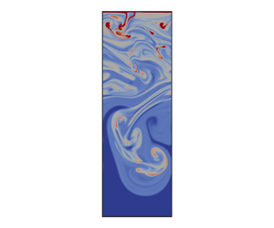
Figure 2 depicts the flow evolution for the representative value of  $Ra = 2.9 \times 10^{-5}$. Figure 2(a–e) shows the early time $t=5000$, with a diffusively growing cold temperature boundary layer at the top whose thickness grows proportionally to $\sqrt {t}$ (Bednarz et al. Reference Bednarz, Lei and Patterson2009). This boundary layer has not yet reached the critical thickness required for convective instability to set in. The solubility in this cold boundary layer is reduced, so that crystals precipitate out. The resulting crystal front propagates downwards in a stable fashion, with the Stokes settling velocity of the individual crystals. We remark that we identified the front locations as peaks in the vertical derivative of the horizontal average of $\rho$.

Figure 2. Two-dimensional fields of the (a, f) velocity magnitude  $||\boldsymbol {u}||$, (b,g) temperature $T$, (c,h) solute salt $S$, (d,i) crystal salt $C$ and (e,j) density $\rho$, for $Ra = 2.9 \times 10^{-5}$. We observe the formation of a distinct temperature front, indicated by the red arrow, and a separate front of settling crystals shown by a grey arrow, at (a–e) $t=5000$ and ( f–j) $40\,000$. The convective front propagates downwards more slowly than the settling particles.
Shortly after the time shown in figure 2(a–e), the temperature boundary layer becomes convectively unstable. Consequently, due to the random perturbations added to the temperature boundary condition, we observe the formation of downwards propagating plumes, which can be seen in Figure 2( f–j) for time  $t=40\,000$. We note that these plumes do not catch up with the particle front, so that two distinct fronts continue to exist.
Figure 3 shows the corresponding flow field for  $Ra = 5 \times 10^{-4}$, corresponding to a larger cooling rate. Early on, the diffusive propagation velocity of the temperature front is still smaller than the crystal settling velocity, so that we again observe the formation of two distinct fronts early on ( $t=1680$). As in figure 2, the diffusively growing cold layer has not yet reached the thickness required for instability. However, for this larger $Ra$ value, the convective instability sets in earlier in time, after which the thermal front propagates downwards more rapidly than the crystal front. Eventually, the temperature front catches up to the crystal front, and the two fronts recombine into a single front by $t=13\,400$. The propagation velocity of this single front is governed by the combined effects of the density gradients due to temperature and crystal concentration (figure 5b). It propagates faster than the two separate fronts individually, suggesting that the particles sediment faster than the Stokes settling velocity of an individual particle, as expected for particles that are advected by the fluid.

Figure 3. Two-dimensional fields of the (a, f) velocity magnitude  $||\boldsymbol {u}||$, (b,g) temperature $T$, (c,h) solute salt $S$, (d,i) crystal salt $C$ and (e,j) density $\rho$, for $Ra = 5 \times 10^{-4}$. At the early time (a–e) $t=1680$, we observe distinct temperature (red arrow) and crystal (grey arrow) fronts. However, by ( f–j) $t=13\,400$, the convectively unstable temperature front has caught up with the crystal front, and the two fronts have combined into one.
For an even larger value,  $Ra = 1.2 \times 10^{4}$, figure 4 shows that two distinct fronts never form. The crystals cannot outrun the evolving temperature front even during the early stages. As a result, even early on, only one unstable density front exists whose propagation in time is governed by the combined effects of temperature, solute salt and crystal concentration gradients. This combined front propagates downwards more rapidly than the Stokes settling velocity of the crystals (figure 5c). Timelapse movies of the flows presented in figures
2–4 are given in the supplementary material.
$Ra = 1.2 \times 10^{4}$, figure 4 shows that two distinct fronts never form. The crystals cannot outrun the evolving temperature front even during the early stages. As a result, even early on, only one unstable density front exists whose propagation in time is governed by the combined effects of temperature, solute salt and crystal concentration gradients. This combined front propagates downwards more rapidly than the Stokes settling velocity of the crystals (figure 5c). Timelapse movies of the flows presented in figures
2–4 are given in the supplementary material.

Figure 4. Two-dimensional fields of the (a, f) velocity magnitude  $||\boldsymbol {u}||$, (b,g) temperature $T$, (c,h) solute salt $S$, (d,i) crystal salt $C$ and (e,j) density $\rho$, for $Ra = 1.2 \times 10^{4}$. We observe a single combined temperature and crystal front both for the early time (a–e) $t=0.3$ (stretched in the vertical direction by a factor of 3 to show the instability at the top) and for the late time ( f–j) $t=3$.

Figure 5. Vertical location of the temperature and crystal concentration fronts as functions of time for:(a) small  $Ra=2.9\times 10^{-5}$, where the two fronts remain distinct for all times; (b) intermediate $Ra=5\times 10^{-4}$, where the crystal front initially outruns the temperature front, but the latter catches up with the former after some time and they recombine; (c) large $Ra=1.2\times 10^4$, where one combined front is observed at all times. The black lines represent the Stokes settling velocity of the crystals, whereas the coloured dots indicate the location of the temperature/combined fronts, showing that in panel (a), the crystals sediment at their Stokes settling velocity, and in panel (b,c), they effectively sediment faster than that. The grey line in panel (a) is a fit over the propagation of the thermal convective front according to (4.8). (d) Phase diagram of the flow regimes for different $Ra$ and diffusivity ratios $\tau$. The simulation presented in figure 6 corresponds to the single blue dot at $\tau =1/40$ in the phase diagram. The colour scheme is consistent in all simulations, and dots denote individual simulations.

Figure 6. Location of the (a) crystal and (b) thermal fronts in time, for  $\tau _S=\tau _C=1/40$ (green) and $\tau _S=\tau _C=1$ (blue). The other parameter values are kept constant at $Ra=7.9\times 10^{-3}$, $Pr=7.1$. The front locations remain close to each other, even after convection starts at approximately $t=400$.
To explore the influence of the diffusivity ratios  $\tau _S$ and $\tau _C$ on the overall evolution of the flow, we conducted additional simulations with $\tau _S = \tau _C = 0.5$ and 0.25. Lower values of $\tau$ imply that the diffusion of temperature is faster than that of salinity and crystals, so that the steepness of the thermal density front declines more rapidly than that of the crystal front. However, the simulations did not show a substantial influence of this effect on the interaction of the two fronts (figure 5d).
This finding is confirmed by two simulations that employ a much finer mesh with  $4200\times 21\,000$ grid points. The first simulation has $\tau _S=\tau _C=1$ ( $Sc=7.1$), while the second one has $\tau _S = \tau _C=\frac {1}{40}$ ( $Sc=284$). This corresponds to Lewis numbers of $1$ and $40$, respectively, for both soluble salt and crystals. All parameters but $\tau _S$, $\tau _C$ and $Sc$, including the boundary condition perturbations, were identical in both simulations; $Ra=7.9\times 10^{-3}$, $Pr=7.1$ and $\beta _S=\beta _C=0.522$.
Figure 6 shows the thermal and crystal front locations as functions of time for both simulations. We observe only minor differences between the front velocities of the two simulations, which confirms our hypothesis that double diffusion does not play a major role in the flowfield under consideration.
3.2. Phase diagram
Consistent with the above observations, we identify three distinct flow regimes, as shown in figure 5. For large Rayleigh numbers, a single combined temperature and crystal concentration front forms from the very beginning, whereas for small Rayleigh numbers, the crystal front outruns the temperature front, and the two fronts remain separate at all times. For intermediate Rayleigh numbers, the crystal front initially descends more rapidly than the temperature front, but after some time, the latter catches up with the former, so that a combined front emerges. For the range of parameter values explored here, the Rayleigh number at which each of these transitions occurs does not seem to depend on the diffusivity ratio  $\tau$.
We remark that if the crystals did not have a settling velocity, their precipitation would not affect the density distribution, since the crystals are assumed to have the same expansion coefficient as the dissolved salt. Hence, under those conditions, the density would vary with temperature only. However, if the crystals have a finite settling velocity, they will sediment out of the colder surface boundary layer, thereby reducing its excess density. Consequently, we expect that particle settling will cause the colder surface boundary layer to go unstable later in time, and with a smaller growth rate. Hence, faster settling of the crystals not only speeds up the crystal front propagation, but it also reduces the velocity of the thermal front.
The vertical black lines in figure 5(d) indicate the approximate values at which the transition between the different flow regimes occurs. The transition from two fronts that do not recombine to two fronts that merge occurs at  $Ra\approx 3\times 10^{-4}$. The second transition, from two fronts that recombine to a single one at all times, takes place near $Ra\approx 6.5$. In the absence of an analytical expression for the propagation velocity of the convectively unstable thermal front, it would be difficult to estimate these transition values.
4. Discussion
In the following, we make an attempt to develop simplified scaling arguments to estimate the approximate  $Ra$ values at which the regime transitions identified in figure 5 occur. For clarity, we denote dimensionless quantities by primes.
4.1. Diffusive behaviour of the thermal front
The transition from diffusive to convective behaviour of the thermal front occurs once the local Rayleigh number  $Ra_{loc}$, formed with the thickness and density difference of the cool surface layer, exceeds a critical value. For the purpose of defining this local Rayleigh number, let us consider the location $y'=-h'_{T,diff}$ where the diffusive temperature is the average between the values at the surface and far below the surface, i.e. $T'(y'=-h'_{T,diff}) = 0.5 T'(y'=0)$. From Bednarz et al. (Reference Bednarz, Lei and Patterson2009), the dimensionless $T$-profile is $T'(y')=-2\sqrt {{t'}/{{\rm \pi} }}\exp ({-({y'^2}/{4t'})})+y'\textit {erfc}({-y'}/{2\sqrt {t'}})$, which gives for the surface temperature $T'(y'=0)=-2\sqrt {{t'}/{{\rm \pi} }}$. Hence, we numerically obtain for the dimensionless thickness of the cool surface layer
 \begin{equation} h'_{T,diff}\left(t'\right) \approx 0.7\sqrt{t'}, \end{equation}
which is valid as long as the thermal front propagates diffusively. The local Rayleigh number  $Ra_{loc}$, formed with the dimensional layer thickness $h'_{T,diff}({\kappa _T}/{v_{s}})$, is therefore
 \begin{equation} Ra_{loc} = \frac{g {\rm \Delta}\rho \left(h'_{T,diff}\dfrac{\kappa_T}{v_{s}}\right)^3}{2 \rho_0 \kappa_{T} \nu}. \end{equation}
By substituting  ${\rm \Delta} \rho =\rho _0\alpha ({T(y=0)}/{2})=\rho _0\alpha \big|{\partial T}/{\partial y}|_{0}({\kappa _T}/{v_{s}})\big|\sqrt {{t'}/{{\rm \pi} }}$ in dimensional form, and using $Ra=-g({\alpha ({\partial T}/{\partial y})|_{0}\kappa _T^3}/{v_{s}^{4} \nu })$, we obtain
 \begin{equation} Ra_{loc} = Ct'^2Ra, \end{equation}
where  $C$ is a constant of $O(1)$. From analogy with classical Rayleigh–Bénard convection, we estimate that the thermal front will become convectively unstable when $Ra_{loc} \approx O(10^3)$, which yields for the time $t'_c$ at which convection commences
 \begin{equation} t'_c \approx 30 Ra^{{-}1/2}, \end{equation}
which is similar to the relation obtained by Lei & Patterson (Reference Lei and Patterson2005). For the case with  ${Ra = 2.9 \times 10^{-5}}$ shown in figure 5(a), this yields $t'_c \approx 6 \times 10^3$, which is in good agreement with simulation data, as shown in figure 7.


4.2. Convective behaviour of the thermal front
In the following, we explore the extent to which simple models of the temperature profile in the convective region, and of the dependence of the convective front velocity on this temperature profile, can reproduce the numerically observed dependence of the convective front location on time. Based on the representative horizontally averaged temperature profiles shown in figure 8(a–c), we approximate these profiles in the convective plume region as being linear functions of depth, reaching  $T'=0$ at the convective front ${y'=-h'_{T,conv}}$,
 \begin{equation} T'\left(y'\right)\propto{-}C_1\left(t'\right) \left(y' + h'_{T,conv}\right), \end{equation}
where  $C_1$ is a function of time only. Conservation of thermal energy implies that the temporal integral of the surface heat flux equals the change in thermal energy across the water column. Any diffusive heat flux below the convective layer is very small and can be neglected, so that we obtain
 \begin{equation} \int_0^t \kappa_T \left.\frac{\partial T}{\partial y}\right|_{0} {\rm d} t \propto \int_{{-}h_{T,conv}}^0 T\left(y\right){{\rm d}y} \end{equation}
in dimensional form. In dimensionless form, this yields  $\frac {1}{2} C_1(t') h'^2_{T,conv}\propto t'$.

Figure 8. Horizontal averages of the temperature profile (black lines) for three different times of the simulation shown in figure 2: (a)  $t'=15\,000$, (b) $t'=27\,000$, (c) $t'=71\,000$. Also shown are linear fits of $T'(y')$ in dashed blue. Black dots in panel (d) denote the slopes of the linear fits of the temperature profile as a function of time, alongside a theoretical line $C_1\propto t'^{-({1}/{3})}$, showing good agreement between the two. Red dots denote the times presented in panel (a–c).
By assuming that the convective front propagation velocity scales with the horizontally averaged vertical temperature gradient in the convective region
 \begin{equation} \frac{{\rm d} h'_{T,conv}}{{\rm d} t'} \propto C_1\left(t'\right), \end{equation}
we obtain
 \begin{equation} h'_{T,conv}\propto t'^{2/3}. \end{equation}
This functional dependence is indicated by the grey line in figure 5(a), and it agrees well with the simulation data for the convective front location in the aforementioned simulation. It follows that  $C_1 \propto t'^{-({1}/{3})}$, which is consistent with this simulation data, as shown in figure 8(d). We remark that we did not observe the above scaling relations for all of the simulations we conducted, so that further work is needed to establish the degree to which these scaling considerations have general applicability.
4.3. The fronts separate and merge
A cooling front is expected to diffuse downwards with a velocity that is proportional to  $t'^{-({1}/{2})}$ from the theory of diffusive processes and the boundary condition at the top, so the front velocity theoretically diverges at very early times. Since the water is saturated with salt, crystals will nucleate at the front due to the temperature drop, producing a single combined density front. Once the propagation of the thermal front will slow down to below the crystal settling velocity, i.e. ${\textrm {d} h'_{T,diff}}/{\textrm {d} t'}=1$, the crystals will depart from the thermal front and propagate ahead of it. From (4.1), this departure is expected to happen at time $t'=0.12$. The thermal front becomes convective at $t'=t'_c$ and will merge with the crystals afterwards, at sufficiently large $Ra$ numbers. Figure 9 depicts the fronts in time for a simulation with $Ra=4$, for which $t'_c\approx 15$, showing a crystal front propagating ahead of the thermal one during the predicted times $0.12< t'< t'_c$.

Figure 9. Thermal (red) and crystal (grey) front locations as functions of time, for a simulation with  ${Ra=4}$. The predicted time for the separation of the crystal front from the thermal one is $t'\approx 0.12$. The onset of convection happens at $t'\approx 10$ and soon afterwards, the fronts merge, in reasonable agreement with the predicted time of $t'_c\approx 15$.
4.4. Application to the Dead Sea
The simulations in figure 5(d) investigate the  $Ra$ range from $1.2\times 10^{-5}$ to $1.2\times 10^{4}$. In the following, we explore the applicability of these results to the conditions of the Dead Sea, which represents the largest hypersaline lake on Earth today (Arnon, Selker & Lensky Reference Arnon, Selker and Lensky2016; Sirota et al. Reference Sirota, Enzel and Lensky2017; Ouillon et al. Reference Ouillon, Lensky, Lyakhovsky, Arnon and Meiburg2019). Recent heat flux measurements (Hamdani et al. Reference Hamdani, Assouline, Tanny, Lensky, Gertman, Mor and Lensky2018; Lensky et al. Reference Lensky, Lensky, Peretz, Gertman, Tanny and Assouline2018) show typical values near $400$ W m $^{-2}$ outwards during winter that last over several hours around sunset. For a density $\rho _0=1240$ kg m $^{-3}$, thermal conductivity 0.8 W K $^{-1}$ m $^{-1}$ (Ben-Avraham, Hänel & Villinger Reference Ben-Avraham, Hänel and Villinger1978) and heat capacity $C_p=3030$ J kg $^{-1}$ K $^{-1}$, we obtain a surface temperature gradient ${\partial T}/{\partial y}|_0=-380$ K m $^{-1}$, assuming purely conductive heat flux. A representative halite crystal radius in the Dead Sea is $10^{-4}$ m (Sirota et al. Reference Sirota, Enzel, Mor, Moshe, Eyal, Lowenstein and Lensky2021), for which Lensky et al. (Reference Lensky, Hochman, Moshe and Bodzin2013) measure a typical settling velocity $v_s=6.2\times 10^{-3}$ m s $^{-1}$. This gives $Ra = 3.1\times 10^{-6}$ over some $10^6$ dimensionless time units which, according to figure 5(d), corresponds to two distinct density fronts that do not recombine, so that the crystals sediment with their settling velocity. However, we need to keep in mind the various assumptions underlying our analysis, such as thermodynamic equilibrium, monodisperse crystals and a limited range of $\tau$-values. Hence, it will be important to validate the above prediction by field measurements.
5. Summary and conclusions
When a saturated layer of brine is cooled from above, a top-heavy density profile forms due to the cold boundary layer at the top. Initially, this boundary layer grows diffusively, but upon reaching a critical thickness, it becomes unstable, giving rise to convection and a downwards propagating cold front. In addition to modifying the fluid density near the top, the surface cooling also reduces the solubility of salt, so that halite crystals precipitate out and sediment, leaving behind less saline brine. This loss of salinity reduces the overall density of the surface layer, but it results in a downwards propagating front of halite crystals. Hence, there are two distinct mechanisms by which surface cooling can generate top-heavy density fronts in saturated brine.
By rendering the governing equations dimensionless, we found that the dominant dimensionless parameter can be cast in the form of a Rayleigh number. We then employed two-dimensional simulations that reproduce the emergence and interaction of the temperature and crystal concentration fronts, and depending on the value of the above dimensionless parameter, we observed the existence of three distinct flow regimes: for small Rayleigh numbers, the two fronts remain distinct at all times and the effective sedimentation velocity of the crystals is their Stokes settling velocity; for intermediate Rayleigh numbers, the crystal front initially outruns the temperature front, but the latter catches up to the former after some time and they recombine; for large Rayleigh numbers, one combined front is observed at all times. The effective sedimentation velocity of the crystals after recombination is hence faster than the Stokes settling velocity.
Based on numerical observations and simple model assumptions about the temperature profile in the convective region, and for the dependence of the convective front velocity on this profile, we furthermore propose approximate scaling laws for the propagation of the thermal and crystal fronts in each regime. We compare these with the simulation data, with generally good agreement.
We note that in the present investigation, we assumed monodisperse halite crystals with a Stokes settling velocity that is constant in space and time. In real world applications, we expect the crystal size distribution to be polydisperse and the crystals to grow in time, so that their settling velocity will change (Lensky et al. Reference Lensky, Hochman, Moshe and Bodzin2013). Moreover, our assumption of thermodynamic equilibrium does not account for supersaturation in the system, and hence there is no delay in the formation of crystals. These effects may modify the above simulation data to some extent, so that it will be useful to conduct field measurements for comparison. Such experiments are currently being planned.
Supplementary material
Supplementary material is available at https://doi.org/10.1017/jfm.2023.809.
Acknowledgements
Several insightful comments by the anonymous reviewers contributed to improvements of the manuscript. E.M. gratefully acknowledges the hospitality of the Hebrew University of Jerusalem, along with financial support through a Lady Davis fellowship. This study was furthermore funded through grants ISF-1471/18, BSF-2019/637, NSF-1936358 and ARO-W911NF-18-1-0379. Finite-volume simulations were conducted using the OpenFOAM buoyantBoussinesqPimpleFoam tool kit, http://www.openfoam.com/, and images of two-dimensional field profiles were generated using ParaView, https://www.paraview.org/ and Adobe Illustrator http://www.adobe.com/.
Declaration of interests
The authors report no conflict of interest.


 Open access