


1. Introduction
In recent years, interest in non-trivial forms of fluid particles was stimulated by applications of non-spherical microparticles to have important potential as building blocks for self-assembled materials, including clustering of cells, imaging probes for therapy, drug carriers, and more (see e.g. Champion, Katare & Mitragotri Reference Champion, Katare and Mitragotri2007; Yan Reference Yan2015; Zabarankin & Grechuk Reference Zabarankin and Grechuk2017). One of the advanced methods for producing microparticles of complex shapes is the solidification of drops deformed by the flow in microfluidic devices. The flow affecting the deformation of a microdrop, can be approximated by a linear one. The resulting linear flow can have shear and rotational components. Systems that may involve such simultaneous components can be found also in multiphase polymer processing such as injection moulding or cases where two impinging jets collide. Further examples of industrial devices in which domains that have a combination of such rotation and extension components are rotary pumps Dmytriv et al. (Reference Dmytriv, Lanets, Dmytriv and Horodetskyy2021) and cyclone separators Li, Huang & Li (Reference Li, Huang and Li2023).
There has been an enormous body of publications concerning the deformation of a drop embedded in a viscous domain and subject to a linear flow field. A comprehensive review of the early studies can be found in Stone (Reference Stone1994). In particular, when a viscous drop, initially spherical at rest, is deforming in an extensional or shear flow, the works of Taylor (Reference Taylor1932), Rallison & Acrivos (Reference Rallison and Acrivos1978) and Hinch & Acrivos (Reference Hinch and Acrivos1980) suggest that with increasing flow rate, the drop can reach a critical shape at which it loses its stable form and beyond which its shape becomes unstable in the flow. A similar transition is found by Acrivos & Lo (Reference Acrivos and Lo1978) for a slender body in extensional flow where more than one branch of the solution of the equations of motion, and more than one stationary shape, stable and unstable, are reported for given flow conditions.
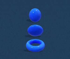
The study of rotating liquid drops has been performed by several authors experimentally, theoretically as well as numerically (see e.g. Chandrasekhar Reference Chandrasekhar1965; Brown & Scriven Reference Brown and Scriven1980; Fontelos, García-Garrido & Kindelán Reference Fontelos, García-Garrido and Kindelán2011; Lyttleton Reference Lyttleton2013; Nurse, Coriell & McFadden Reference Nurse, Coriell and McFadden2015; Elms et al. Reference Elms, Hynd, Lopez and McCuan2017; Holgate & Coppins Reference Holgate and Coppins2018). The computational study of equilibrium shapes of such drops was conducted by Poincaré (Reference Poincaré1885) and Appell (Reference Appell1932). According to Poincaré (Reference Poincaré1885), two families of solutions could be obtained, which consist of axisymmetric and asymmetric shapes. A detailed classification of all rotationally symmetric figures of equilibrium corresponding to rotating liquid masses subject to surface tension was given in Elms et al. (Reference Elms, Hynd, Lopez and McCuan2017). Fontelos et al. (Reference Fontelos, García-Garrido and Kindelán2011) studied the stationary shapes, evolution and breakup of a viscous rotating drop, making use of the Stokes model and a boundary integral approach. Multiple axisymmetric solutions were found for a range of governing parameters. Ellipsoidal, flat dimpled and toroidal shapes may exist for the same flow conditions.
The multiplicity of stationary shapes of drops deforming in a linear compressional flow was also reported in Zabarankin et al. (Reference Zabarankin, Smagin, Lavrenteva and Nir2013), Zabarankin, Lavrenteva & Nir (Reference Zabarankin, Lavrenteva and Nir2015) and Ee et al. (Reference Ee, Lavrenteva, Smagin and Nir2018). There, the reported branches of solutions were either stable stationary flat drops or unstable yet stationary toroidal drops. These predictions comprise dual branches of stationary solutions, resulting at a given capillary number, but they appeared to be unconnected, in contrast to the drops deforming in a rotational flow field, where the stationary branches of flat and toroidal drops are connected by a branch of flat discs having ever-growing dimples (Fontelos et al. Reference Fontelos, García-Garrido and Kindelán2011). Lavrenteva et al. (Reference Lavrenteva, Ee, Smagin and Nir2021) proposed to approximate stationary shapes of the drops in compressional flow by using generalized Cassini ovals. The analysis reproduced the branches with shapes of stationary stable flat drops and stationary unstable toroidal drops, available from numerical calculation, and predicted the transition branch between oval and toroidal shapes, consisting of flat drops with ever-growing dimples up to collapse.
Malik, Lavrenteva & Nir (Reference Malik, Lavrenteva and Nir2020) considered deformation of an immiscible drop in a linear flow that is composed of two simultaneous components, rotational flow and axisymmetric flow, either compressional or extensional. The dynamic deformation, stationarity and stability with respect to axisymmetric perturbation were characterized using dimensionless parameters such as the Bond number and capillary number. A domain in the phase plane of the Bond number and the capillary number within which the deformed drop will be stable is obtained. Malik, Lavrenteva & Nir (Reference Malik, Lavrenteva and Nir2021) reported on the branch of toroidal stationary shapes existing under the same conditions as simply connected ones. Malik et al. (Reference Malik, Lavrenteva, Idan and Nir2022) used a feedback-control approach to extend the branch of toroidal drops up to near collapse. Yet the branches of singly connected and toroidal shapes remained unconnected in cases with and without rotation.
The main goal of this study is to construct the connecting branch in the case when the outer linear flow consists of rotational and axisymmetric (extensional or compressional) components. The method that was employed is based on the use of classical control theory similar to that employed in Malik et al. (Reference Malik, Lavrenteva, Idan and Nir2022). Methods of control theory are employed extensively and successfully to stabilize various types of flow, e.g. for controlling the onset of turbulence, and turbulence suppression in channel and pipe flow. A comprehensive review of the modern state of this subject can be found in Jovanović (Reference Jovanović2021). Fikl & Bodony (Reference Fikl and Bodony2021) developed optimal control methods for stationary and time-dependent deformation of a drop in viscous flow.
In the present study, a simple proportional-integral controller is used. The intensity of the extensional component of the outer flow is chosen for a control signal. The controller is designed using a simplified model of the system and employed for the full model, demonstrating sufficient robustness. In § 2, we give the mathematical model used for the analysis. The design of the controller based on a simplified model of the process is described in § 3. Section 4 presents the implementation of the controller to the full (boundary integral) dynamic problem. A discussion of the results concerning stationary solutions is given in § 5, followed by concluding remarks in § 6.
2. Problem formulation and solution methodology
2.1. Drop dynamics in linear viscous flow
We consider a viscous drop of fixed volume  $V=4{\rm \pi} l^3/3$ embedded in an immiscible unbounded viscous fluid, where $l$ is the radius of the undeformed spherical drop. Let the domain occupied by the drop be denoted by $\varOmega _1$, and let the unbounded external domain be defined by $\varOmega _2$. The viscosity and density of the drop and the ambient fluid are represented by $\mu _1, \rho _1$ and $\mu _2, \rho _2$, respectively. The velocity and pressure fields in $\varOmega _i$, $i=1,2$, are denoted as ${\boldsymbol {u}}_i, p_i$, respectively. The drop and external fluid are supposed to rotate in an axisymmetric manner around a common axis with angular velocity $\omega$.
In this study, the external flow is considered to be extensional or compressional in combination with rotation. In the reference frame rotating with the angular velocity  $\omega$, the velocity of external flow, in the absence of a drop, is
 \begin{equation} u_i^0= G_{ij}x_j, \end{equation}
where  $G_{11}=G_{22}=G$, $G_{33}=-2G$, and $G_{ij}=0$ whenever $i \neq j$. Here, $G$ denotes a shear rate that characterizes the intensity of the flow, which may be positive or negative, representing the compression and extension modes of the flow, respectively.
In what follows, throughout the paper, non-dimensional variables are used, where  $l$,
$l$,  $U=\gamma /\mu _2$, $\varPi =\gamma /l$ and $T=l/U$ are the length, velocity, pressure and time scales, respectively. The governing parameters of the problem are the viscosity ratio $\lambda = \mu _1/\mu _2$, the capillary number $Ca=\mu _2 G l /\gamma$, and the rotational Bond number $Bo=(\rho _1-\rho _2)\omega ^2 l^3/\gamma$. In the present study, the drop and the ambient fluid are considered to have the same viscosity, i.e. $\lambda =1$.
In this investigation, we explored the realm of creeping incompressible flow conditions, where the viscosities of the drop and the ambient fluid are considered to be same. When inertia and sedimentation effects are ignored, the Stokes system in a rotating frame of reference is given as
 \begin{gather} \boldsymbol{\nabla} \boldsymbol{\cdot} {\boldsymbol{u}}_i=0 \qquad\qquad \text{in}\ \varOmega_i(t), \ i=1,2, \end{gather}
 \begin{gather} {-\boldsymbol{\nabla} P_i} +\Delta {\boldsymbol{u}}_i=0 \quad \text{in}\ \varOmega_i(t), \ i=1,2. \end{gather}
Here,  $P_i$ is the non-dimensional form of modified pressure as given in Fontelos et al. (Reference Fontelos, García-Garrido and Kindelán2011). The stress balance at the drop interface is maintained as
 \begin{equation} \left(\sigma_{1}-\sigma_{2}\right) \boldsymbol{\cdot} {\boldsymbol{n}}={-}\frac{1}{Ca}\left(\kappa-\frac{Bo}{2}\,r^2 \right){\boldsymbol{n}} \quad \text{in} \ \partial \varOmega(t), \end{equation}
where the  $\sigma _i$ denote the interfacial stresses, ${\boldsymbol {n}}$ is the unit normal vector pointing outwards from the drop interface, and $\kappa$ is the surface mean curvature. The non-dimensional parameters $Ca$ and $Bo$ are the capillary and Bond numbers, respectively. At the interface of the drop ( $\delta \varOmega$), the velocity ( ${\boldsymbol {u}}_s$) is assumed to be equal to the velocity of the ambient fluid, i.e.
 \begin{equation} {\boldsymbol{u}}_1={\boldsymbol{u}}_2={\boldsymbol{u}}_s. \end{equation}
The dynamics of this surface is determined by the kinematic condition
 \begin{equation} u_n={\boldsymbol{u}}_s \boldsymbol{\cdot} {\boldsymbol{n}} \quad \text{on} \ \partial \varOmega(t), \end{equation}
where  $u_n$ denotes the velocity of the surface in the normal direction. Far from the drop,
 \begin{equation} {\boldsymbol{u}}_2 \rightarrow Ca\,{\boldsymbol{u}}^\infty \quad \textrm{when}\ |{\boldsymbol{x}}| \rightarrow \infty, \quad{\boldsymbol{u}}^\infty= (x_1, x_2, -2 x_3). \end{equation}
 It should be noted that the parameters  $Ca$ and $Bo$ can assume positive as well as negative values. Here, the positive and negative values of $Ca$ represent the compressional and extensional flow, respectively. When $Bo$ is positive, the drop density exceeds the density of the ambient fluid, which we call a heavy drop; and when $Bo$ is negative, the density of the ambient fluid exceeds the drop density, which we call a light drop.
2.2. Boundary integral formulation
For a given shape of the drop, the problem (2.2)–(2.5), (2.7) can be formulated as a system of integral equations for the velocity at the interface  $\partial \varOmega$ as given by Rallison & Acrivos (Reference Rallison and Acrivos1978) and Pozrikidis (Reference Pozrikidis1992). In the case of equal viscosity of the phases, the velocity at the interface is given by an explicit expression,
 \begin{equation} u_j({\boldsymbol{x}}_p)=Ca \, u^\infty_j({\boldsymbol{x}}_p)-\frac{1}{8{\rm \pi}}\int_{\partial \varOmega} \left(\kappa ({\boldsymbol{x}})-\frac{Bo \,r^2}{2} \right) n_i({\boldsymbol{x}})\, J_{ij}({\boldsymbol{x}}-{\boldsymbol{x}}_p) \,{\rm d}S(x), \end{equation}
where  ${\boldsymbol {x}}_p$ denotes the position vector of any point $p$ on the surface, and
 \begin{equation} J_{ij}(\kern0.7pt\boldsymbol{y})=\frac{\delta_{ij}}{|{\boldsymbol{y}}|}+\frac{y_i y_j}{|{\boldsymbol{y}}|^3}. \end{equation}
Recall that  ${\boldsymbol {u}}^\infty (\kern0.7pt\boldsymbol{y})=(y_1,y_2,-2 y_3)$, and the positive and negative signs of $Ca$ refer to compressional and extensional flow, respectively. Here, $\delta _{ij}$ is the Kronecker delta. In this study, $y_3=z$, and the $z$-axis is considered to be the axis of rotation. The pressure and velocity are independent of azimuth angle $\phi$ in the cylindrical coordinates $(r, z, \phi )$. Equation (2.8) can be integrated over the angular coordinate and reduced to expressions for the components of the velocity at the interface in cylindrical coordinates containing curvilinear integrals over the cross-section of the drop interface $L$:
$L$:
 \begin{align} u_j(r_p, z_p) &= Ca \,
u^\infty_j(r_p, z_p) -\frac{1}{8{\rm \pi}}\int_{L} \left(\kappa
(r, z)-\frac{Bo\,
r^2}{2} \right)\nonumber\\
&\quad\times n_i(r, z)\,M_{ij}(r_p, z_p, r, z) \,{\rm
d}L, \quad j=r, z.
\end{align}
\begin{align} u_j(r_p, z_p) &= Ca \,
u^\infty_j(r_p, z_p) -\frac{1}{8{\rm \pi}}\int_{L} \left(\kappa
(r, z)-\frac{Bo\,
r^2}{2} \right)\nonumber\\
&\quad\times n_i(r, z)\,M_{ij}(r_p, z_p, r, z) \,{\rm
d}L, \quad j=r, z.
\end{align} The resulting expressions for the kernels  $M_{ij}$ can be found in Pozrikidis (Reference Pozrikidis1992). The simulation process of dynamic deformation starts with the solution for some given shape of a singly connected drop of volume $4{\rm \pi} /3$. At each time step, the velocity at the interface is computed from (2.10), and the drop's surface is updated accordingly in the normal direction in a quasi-stationary manner with the help of the kinematic condition (2.6). The detailed literature concerning this approach can be found in Zabarankin et al. (Reference Zabarankin, Smagin, Lavrenteva and Nir2013), where it was used for simulating the dynamic deformations of a drop in a compressional flow in the absence of rotation, $Ca>0$, $Bo=0$. The same approach was employed recently by Malik et al. (Reference Malik, Lavrenteva and Nir2020) to study deformation of a drop under the combined action of rotation and compressional or extensional flow. It was demonstrated that for every pair $(Bo, Ca)$, the drop either stabilizes to a stationary shape or eventually breaks up.
2.3. Stationary drop shapes
The drop is of stationary shape if the normal velocity at its interface vanishes, that is,
 \begin{equation} u_n ={\boldsymbol{u}}_s \boldsymbol{\cdot} {\boldsymbol{n}} = 0. \end{equation}
In the dynamic computations (Zabarankin et al. Reference Zabarankin, Smagin, Lavrenteva and Nir2013; Malik et al. Reference Malik, Lavrenteva and Nir2020), the solution was assumed to be stationary if (2.11) was established to a desired degree of accuracy. We note that, following Malik et al. (Reference Malik, Lavrenteva and Nir2020, Reference Malik, Lavrenteva, Idan and Nir2022), with a mesh of 100 surface elements, the criterion for stationarity is set at  $\max (|u_n|) \leq O(10^{-3})$. The obtained singly connected stationary shapes do not change for an indefinitely long time, and are addressed as stable with respect to axisymmetric perturbations. The region of stable drop shapes in terms of $Bo$ and $Ca$ has been presented in Malik et al. (Reference Malik, Lavrenteva and Nir2020).
In the special case when  $Ca=0$, the velocity field in the laboratory reference frame is just that of a solid body rotation, and the shape of the interface can be found via solving a system of ordinary differential equations (see e.g. Fontelos et al. Reference Fontelos, García-Garrido and Kindelán2011). Analysis of these equations reveals that the solution is not unique. For a certain region of $Bo$, oval shapes coexist with toroidal and flattened, dimpled ones.
An alternative method to find stationary solutions is to use an iterative procedure to minimize a norm of the normal velocity at the interface. For a stationary shape, this minimum should be zero. This method is not necessarily related to the actual dynamics of the drop and can be advantageous in finding unstable shapes. In particular, the effectiveness of such an approach is anticipated when the shape of the drop can be approximated by a simple geometric shape defined by a small number of parameters. Numerous such approximations are available in the literature. Zabarankin et al. (Reference Zabarankin, Smagin, Lavrenteva and Nir2013) suggested several such approximations in the case  $Bo = 0$ and $\lambda = 1$, which were shown to provide excellent fitting to all the stable shapes obtained by the dynamic simulations. Lavrenteva et al. (Reference Lavrenteva, Ee, Smagin and Nir2021) used generalized Cassini ovals to approximate drop cross-sections and find stationary shapes by minimizing a convex functional of normal velocity at the interface. The analysis reproduced the branches with shapes of stationary stable flat drops and stationary toroidal ones available from numerical calculation in the case $Bo = 0$ and $\lambda = 1$. Furthermore, it predicts the point of loss of stability of the flat drop to exhibit the transition branch that leads into the formation of the toroidal shapes, and shows that this branch shows stationary, yet unstable, flat drops with ever-growing dimples up to collapse. However, as it was shown in Malik et al. (Reference Malik, Lavrenteva and Nir2020) that in the presence of rotation, the cross-sections of stationary drops did not always resemble Cassini ovals. Thus another method is required to find the branch of unstable dimpled shapes.
In this paper, we employ a method based on the use of a classical control theory, where the problem is reduced to a dynamical system with a low number of variables (states). We find a stationary solution of this system, linearize the system in the vicinity of this stationary solution, and on the basis of the linearized model, design a linear feedback controller. This controller is then used on the original nonlinear dynamic model of the system. For a control signal, we used the capillary number  $Ca$ that is proportional to the intensity of the outer flow. A similar approach was used in Malik et al. (Reference Malik, Lavrenteva, Idan and Nir2022) to stabilize toroidal drop shapes. Detailed descriptions of the algorithm and obtained results are presented in the forthcoming sections.
3. Design of the control
3.1. Simplified model for axisymmetric drop dynamics
Consider a two-parameter family of singly-connected bodies of rotation having the same volume as a unit sphere. Let the cross-section  $L$ of the surface of a body of this family be described by the parametric equations
 \begin{equation} r=a_1 \cos \theta,\quad z= \sin \theta\,(a_2 +a_3 P_1(2 \sin \theta -1)), \end{equation}
where  $\theta \in [0,{\rm \pi} /2]$, and the coefficients $a_k$ satisfy
 \begin{equation} a_1^2 (a_2 + 2 a_3)= 2 \end{equation}
to ensure that the volume of the drop is equal to that of the unit sphere.
In what follows, we use the notation
 \begin{equation} R_{max}=r(0)=a_1, \quad Z_0=z({\rm \pi}/2)=a_2+a_3. \end{equation}
To construct the dynamic equations for these two parameters, we use the kinematic conditions at  $\theta = 0$ and ${\rm \pi} /2$, i.e. at the points on the interface with coordinates $(R_{max},0)$ and $(0,Z_0)$, and take $R_{max}(t)$ and $Z_0(t)$ for the states of the dynamic system. Due to the symmetry of the interface, at $(R_{max},0)$ we have $u_z=0$ and $n_z=0$, while at $(0,Z_0)$ we have $u_r=0$ and $n_r=0$. Thus the dynamic system takes the form
 $$\begin{gather} \frac{{\rm d} R_{max}}{{\rm d} t} = f_1(R_{max}, Z_0, Ca, Bo) =u_r(R_{max},0,Ca,Bo), \end{gather}$$
 $$\begin{gather}\frac{{\rm d} Z_0}{{\rm d} t} = f_2(R_{max}, Z_0, Ca, Bo) =u_z(0,Z_0,Ca,Bo). \end{gather}$$
Here,  $u_r$ and $u_z$ are computed from (2.10), with $L$ defined by (3.1), where coefficients $a_1$, $a_2$ and $a_3$ are given by
 \begin{equation} a_1=R_{max}, \quad a_2=2 R^{{-}2}_{max}-Z_0, \quad a_3=2(Z_0-R^{{-}2}_{max}). \end{equation}
Note that the right-hand sides of (3.4) are nonlinear functions of the model variables  $R_{max}$ and $Z_0$, and depend also on the flow characteristics defined by $Bo$ and $Ca$. The latter will be utilized when the drop shape control is addressed in the sequel.
3.2. Feedback control to determine stationary solutions
A linear feedback controller is designed using an approximate model of the drop deformation presented in the previous subsection. Consequently, this controller is used for the nonlinear dynamic model formulated in § 2. Since the controller is robust only to limited variations in the model parameters, i.e. in the flow conditions, once the limit of flow variations for which a stationary solution can be found is reached, a new controller is designed for the new stationary solution that is close to that limit. The process is repeated and covers the entire range of flow conditions of interest.
Note that the dynamic model, even the simplified one, is nonlinear. However, since our main goal is to find stationary solutions, and not to perform advanced nonlinear regulation and tracking control tasks, we will employ a linearization-based classical linear control design, using the simple model and a single-input-single-output controller.
In the present study, for any fixed  $Bo$, the control signal is chosen to be $Ca$. In a previous work (Malik et al. Reference Malik, Lavrenteva and Nir2021) it was found that for a fixed $Bo$,
$Bo$,  $R_{max}$ dictates a unique drop shape. Therefore, the dictated control input and the feedback signal that is used by the controller are chosen as $R_{max}$.
The control is designed on the basis of the approximate two-state model described in § 3.1. The states of this model are  $\boldsymbol {x}(t)=(R_{max}(t),Z_0(t))$, and their nonlinear dynamics is governed by (3.4). For the controller design, this model is linearized around a stationary solution denoted by $\boldsymbol {x}^0$, corresponding to $Ca^0$. The linearized model is given by
 $$\begin{gather} \delta \dot{\boldsymbol{x}}=\boldsymbol{A}\,\delta \boldsymbol{x}+ \boldsymbol{B}\,\delta Ca, \end{gather}$$
 $$\begin{gather}\delta R_{max}= \boldsymbol{C}\,\delta \boldsymbol{x} + \boldsymbol{D}\,\delta Ca, \end{gather}$$
where  $\dot {\boldsymbol {x}}$ denotes ${{\rm d}\kern0.7pt x}/{{\rm d}t}$, and
 \begin{align}
\left. \begin{gathered}
\boldsymbol{A}=\left[\dfrac{\partial
\boldsymbol{f}}{\partial \boldsymbol{x}}
\right]_{\boldsymbol{x}^0}=\left[
\begin{array}{cc} \dfrac{\partial f_1}{\partial R_{max}} &
\dfrac{\partial f_1}{\partial Z_0} \\ \dfrac{\partial
f_2}{\partial R_{max}} & \dfrac{\partial f_2}{\partial Z_0}
\end{array} \right],\quad
\boldsymbol{B}=\left[\dfrac{\partial
\boldsymbol{f}}{\partial Ca}
\right]_{\boldsymbol{x}^0}=\left[ \begin{array}{c}
\dfrac{\partial f_1}{\partial Ca} \\ \dfrac{\partial
f_2}{\partial Ca} \end{array} \right]=\left[
\begin{array}{c} R^0_{max} \\ -2 Z^0_0 \end{array}
\right],\\ \boldsymbol{C}=\left[\dfrac{\partial
R_{max}}{\partial \boldsymbol{x}}
\right]_{\boldsymbol{x}^0}=\left[
\begin{array}{cc} \dfrac{\partial R_{max}}{\partial
R_{max}} & \dfrac{\partial R_{max}}{\partial Z_0}
\end{array} \right]=\left[ \begin{array}{cc} 1 & 0
\end{array} \right],\quad \boldsymbol{D}=
\left[\dfrac{\partial R_{max}}{\partial Ca}
\right]_{\boldsymbol{x}^0}=0 .
\end{gathered} \right\} \end{align}
\begin{align}
\left. \begin{gathered}
\boldsymbol{A}=\left[\dfrac{\partial
\boldsymbol{f}}{\partial \boldsymbol{x}}
\right]_{\boldsymbol{x}^0}=\left[
\begin{array}{cc} \dfrac{\partial f_1}{\partial R_{max}} &
\dfrac{\partial f_1}{\partial Z_0} \\ \dfrac{\partial
f_2}{\partial R_{max}} & \dfrac{\partial f_2}{\partial Z_0}
\end{array} \right],\quad
\boldsymbol{B}=\left[\dfrac{\partial
\boldsymbol{f}}{\partial Ca}
\right]_{\boldsymbol{x}^0}=\left[ \begin{array}{c}
\dfrac{\partial f_1}{\partial Ca} \\ \dfrac{\partial
f_2}{\partial Ca} \end{array} \right]=\left[
\begin{array}{c} R^0_{max} \\ -2 Z^0_0 \end{array}
\right],\\ \boldsymbol{C}=\left[\dfrac{\partial
R_{max}}{\partial \boldsymbol{x}}
\right]_{\boldsymbol{x}^0}=\left[
\begin{array}{cc} \dfrac{\partial R_{max}}{\partial
R_{max}} & \dfrac{\partial R_{max}}{\partial Z_0}
\end{array} \right]=\left[ \begin{array}{cc} 1 & 0
\end{array} \right],\quad \boldsymbol{D}=
\left[\dfrac{\partial R_{max}}{\partial Ca}
\right]_{\boldsymbol{x}^0}=0 .
\end{gathered} \right\} \end{align}
The partial derivatives in the expression for  $\boldsymbol {A}$ are calculated numerically using a second-order central difference scheme.
The open-loop transfer function between the control input  $\delta Ca$ and the output $\delta R_{max}$, which will be used in the controller design, is given by
 \begin{equation} G_{ol} = \boldsymbol{C}\left(s\boldsymbol{I}-\boldsymbol{A}\right)^{{-}1}\boldsymbol{B}+\boldsymbol{D},\end{equation}
where  $s$ is the complex Laplace variable, and $\boldsymbol {I}$ is a $2\times 2$ identity matrix.
The uncontrolled process corresponds to  $Ca=Ca^0$, i.e. $\delta Ca=0$. If at least one eigenvalue of $\boldsymbol {A}$ in (3.6), or equivalently, one of the poles of $G_{ol}(s)$, has a positive real part, then the stationary solution of (3.4) is unstable. In the current study, we chose $R_{max}$ to be the controlled output variable.
In order to design a controller that stabilizes the system of (3.6) and also can generate a neighbouring solution defined by  $\delta R_{max}^D= R_D- R_{max}^0$, we introduce the error term between the desired and calculated outputs:
 \begin{equation} {e}(t)= R_D - R_{max}= \delta R_{max}^D- \delta R_{max}. \end{equation}
The control input  $\delta Ca$ is chosen in a such a manner that the transfer function in (3.8) does not have a pole at the origin, and to ensure type one characteristics of the closed loop system, a proportional-integral controller is used to stabilize the system (Ogata Reference Ogata2010), given by
 \begin{equation} \delta Ca={-}{K}_p \boldsymbol{e}-{K}_I \boldsymbol{e}_I, \end{equation}
where
 \begin{equation} \dot{\boldsymbol{e}}_I = \boldsymbol{e}. \end{equation}
Here,  ${K}_p$ and ${K}_I$ are proportional and integral gains designed to stabilize the closed loop system. The integral component of the controller is introduced for robustness and to better account for the modelling errors caused by the simplified model. Also, this component will allow us to move from one stationary solution to the neighbouring one.
In the present study, the parameters  ${K}_p$ and ${K}_I$ are designed using the classical root-locus tuning techniques. The transfer function of the controller is given by
 \begin{equation} C(s)=\frac{\delta Ca}{\boldsymbol{e}}(s)=K_p+\frac{K_I}{s}. \end{equation}
The corresponding closed loop transfer function of the system is
 \begin{equation} G_{cl}(s)=\frac{\delta R_{max}}{\delta R_{max}^D}(s) = \frac{G_{ol}(s)\,C(s)}{1+G_{ol}(s)\,C(s)}. \end{equation}
 As discussed earlier, the above controller is used in the vicinity of the stationary solution  $\boldsymbol {x}^0$ to find neighbouring stationary shapes. This is carried out by applying this control logic to the full nonlinear model of the system (2.10). Since the linear controller computes only deviations in the capillary number, the value used in the simulations is given by $Ca=Ca^0+\delta Ca$, as is discussed next.
4. Control implementation to the full boundary integral formulation
For a chosen pair  $(Ca^0, Bo)$, the controller gains $K_p$ and $K_I$ are determined as described in the previous section. Once the controller for the simplified model is established, it is applied to the full nonlinear dynamics model of (2.8) or (2.10) to determine the stationary solution with $R_{max}=R_D$. Namely, in (2.10), the capillary number is changed dynamically as
 \begin{equation} Ca(t)= Ca^0 -{K}_p \left(R_{max}(t)- R_D\right)-{K}_I \int_0^t\left(R_{max}(\tau)- R_D\right){\rm d}\tau, \end{equation}
where
 \begin{equation} R_{max}(t)=\max_{(r,z) \in S_t}(r). \end{equation}
For the initial conditions, we chose the established shape  $S_0$ corresponding to particular $(Ca^0, Bo)$, and set some $R_D$ that is relatively close to $R_{max}^0 =\max _{(r,z) \in S_0}(r)$. If the deviation in $R_{max}$ is sufficiently small and the controller is robust enough, then simulation will converge to a neighbouring solution of the nonlinear model. An example of the controlled dynamics is presented in figure 1. The control was designed for $Bo = 0$ and $Ca_0 = 0.1969$, which is close to the critical point reported in Malik et al. (Reference Malik, Lavrenteva and Nir2020). The corresponding stationary shape has $R_{max} \simeq 1.70648$. The gains were chosen as ${K_p=0.5473}$ and $K_I=0.0274$. Figures 1(a) and 1(b) show the dynamics of $R_{max}-R_D$ and $Ca$, respectively.

Figure 1. Controlled dynamics of (a)  $R_{max}-R_D$ and (b) $Ca$, when $Bo=0$.
In figure 1(a), the dynamics of  $R_{max}-R_D$ is presented. In this presentation, the desired stationary shape of the drop is assumed to be attained when $|R_{max}-R_D|$ approaches zero while the capillary number tends to some constant value. The dynamics for $R_D=1.706472$ (solid blue line) begins with $R_{max}-R_D=0$, and the modification in $Ca(t)$ (see figure 1b) corrects the $R_{max}(t)$ value in order to approach the stationary solution corresponding to the desired shape. Evidently, the difference $R_{max}-R_D$ increases initially, and after a certain time it starts decreasing towards $R_{max}-R_D=0$. In the cases described by the dashed red, dash-dotted yellow and dotted purple lines in figure 1(a), the desired values of $R_{max}$ are obtained successfully in a similar manner. A previously obtained stationary shape is used as an initial shape for simulating the next desired shape. Note that the overshoot and the settling time of $R_{max}-R_D$ are increasing with increasing $R_D$ values. The reason behind this may be the decreasing impact of a particular control on higher values of $R_D$. In figure 1(b), in all cases, $Ca(t)$ settles down quickly, and eventually stabilizes to the $Ca$ values (i.e. $Ca^D$) that maintain $R_{max}=R_D$ as depicted in figure 1(a). Note that all cases of the dynamics illustrated in figure 1 are obtained with the same control.
For non-zero values of the Bond number, an algorithm of receiving stationary solutions is similar: a control designed on the basis of the two-state model for a given pair  $(Bo, Ca^0)$, corresponding to a stationary shape with $R_{max}^0$, when applied to a full system with this very stationary shape as initial condition, converges to a stationary solution with $R_D \in \bigcup (R_{max}^0)$ i.e. in some vicinity of $R_{max}^0$. When the same initial stationary state fails to generate the new desired shape, we use the last obtained stationary shape of the stabilized drop as the initial shape for simulation, with the same controller gain values. As in the case $Bo=0$, in cases where $Bo \neq 0$, we begin with $(Bo, Ca^0)$, close to the critical point report Malik et al. (Reference Malik, Lavrenteva and Nir2020). Note that the instability in drop shape develops faster with the advance along the unstable branch of the solution in any particular case of $Bo$. The stabilization of such ‘more unstable’, i.e. faster diverging, shapes may not be attained with the previously designed controller, $K_P$ and $K_I$ (this is a typical case for $Bo \neq 0$), and is likely to require higher controller gains. At this point, we design a new controller for the updated stationary values corresponding to the new $Ca$ and the corresponding shape. The simulation and stabilization of drops for neighbouring flow conditions are performed considering this new stationary shape. With the help of the procedure described above, we succeeded in obtaining stationary shapes close to those of collapse at the centre of the drop with $Z_0$ as small as $0.01$.
Examples of such controlled dynamics for  $Bo=-5$ are presented in figure 2. The dynamics for $R_D=1.72$ (dashed red lines) begins with the shape given in Malik et al. (Reference Malik, Lavrenteva and Nir2020) with $R_{max}^0$ just a little lower than $R_D$. Then the modification in $Ca(t)$ (see figure 2b) corrects the $R_{max}(t)$ value in order to get the stationary solution corresponding to the desired shape. Evidently, after a short time, $R_{max}$ approaches $R_D$. In the cases described by the dotted yellow lines, dash-dotted purple lines and solid magenta lines (figure 2a), the differences between the initial and desired values of $R_{max}$ are relatively high. For example, in the case described by the dotted yellow line ( $R_D =2.4$), the control designed for $R_{max}^0=1.72$ was employed. In this case, it took much longer time to achieve the stationary state, and one can see oscillations of $R_{max}(t)$ and $Ca(t)$ at the initial period of time reflecting complex eigenvalues of the controlled system. Consequently, in the cases corresponding to the dash-dotted purple and solid magenta lines, new controllers were designed based on the updated stationary states and capillary numbers. This results in faster convergence and less noticeable oscillations.

Figure 2. Dynamics of  $R_{max}(=R_{z=0})$ and $Ca$. (a) Dynamics of $R_{z=0}$ when $Bo=-5$. (b) Dynamics of $Ca$ when $Bo=-5$.
The calculations described below were run up to  $t = 100$, then the normal velocity at the interface was checked. The observed $\max (|u_n|)$ at $t = 100$ was typically $O(10^{-5})$ or less, while in more complex geometry, such as deep dimples or in the vicinity of the region of transition from simply connected to toroidal branches, it was $O(10^{-3})$ or less. The particular levels of accuracy are indicated in the discussions following the results displayed below in § 5.
5. Results and discussion
5.1. Stationary axisymmetrically rotating drops
Malik et al. (Reference Malik, Lavrenteva and Nir2020) reported on dynamic deformation of an immiscible singly connected drop in a linear flow that is composed of two simultaneous components, rotational flow and axisymmetric flow. It was demonstrated that if the Bond number and the capillary number lie within a certain domain in the phase plane, then the drops stabilize to stationary shapes. It has been claimed that outside these bounds, instabilities dominate the drop shapes; hence no stable stationary shapes were obtained. In the present work, we focus on finding new stationary unstable drop shapes. These are attained and stabilized with the help of a control algorithm as described in §§ 3 and 4.
Recall that the control approach starts with an approximation of drop shape close to the desired one that is deforming in the dynamically modified flow field to obtain the shape with a desired characteristic ( $R_{max}=R_D$ in our case). In other words, the control method aims to attain a desired drop shape, defined in terms of length of radial axis ( $R_D$), by modifying the ambient flow field, represented by capillary number $Ca$.
$Ca$.
The obtained stationary drop shapes of the cases depicted in figure 1(a) are shown in figure 3. Drop shapes in these cases of the outer flow corresponding to capillary numbers  $Ca=0.196843, 0.195015, 0.189963, 0.183298$ are shown as solid lines. Approximate solutions of similar cases obtained by Lavrenteva et al. (Reference Lavrenteva, Ee, Smagin and Nir2021), using generalized Cassini ovals, are shown by dashed lines with $Ca=0.196, 0.195, 0.19$, and $0.1831$ for figures 3(a,b,c,d), respectively. The shapes are almost indistinguishable. However, the normal velocities at the interface approximated by the generalized Cassini ovals are of the order $10^{-3}$ (see Lavrenteva et al. Reference Lavrenteva, Ee, Smagin and Nir2021), being several orders of magnitude higher than those associated with the shapes of the present paper in figure 3, i.e. $\max |u_n|=8.5 \times 10^{-6}, 1.5 \times 10^{-5}, 2.0 \times 10^{-5}, 3.3 \times 10^{-5}$, respectively.

Figure 3. Shapes corresponding to  $Bo=0$: (a) $Ca=0.196843$, $R_{max}=1.706473$, $z_{r=0}=0.231444$;(b) $Ca=0.195015$, $R_{max}=1.8$, $z_{r=0}=0.163002$; (c) $Ca=0.189963$, $R_{max}=1.9$, $z_{r=0}=0.088505$; (d) $Ca=0.183298$, $R_{max}=1.985231$, $z_{r=0}=0.009633$. The dashed red curves correspond to the Cassini approximation (Lavrenteva et al. Reference Lavrenteva, Ee, Smagin and Nir2021).
The computations of Malik et al. (Reference Malik, Lavrenteva and Nir2020) revealed that the heavy drops ( $Bo \ge 0$) lose stability with the appearance of a slight dimple at the central part of the drop. In figures 4(a,b,c,d), we present the controlled stationary dimpled shapes of heavy drops for $Bo=4$, and $Ca=0.021656$, $0.012215$, $0.001945$ and $0.000003$, respectively, with $|u_n|_{max} \leq O(10^{-4})$. Note that the case presented by figure 4(d) resembles the shape of the drop for $Bo=4.0004$ with $Ca=0$ as presented in figure 3(d) of Malik et al. (Reference Malik, Lavrenteva and Nir2020). This regenerated result is represented by a dashed line overlapping the present result.

Figure 4. Shapes corresponding to  $Bo=4$: (a) $Ca=0.021656$, $R_{max}=1.5$, $z_{r=0}=0.230345$;(b) $Ca=0.012215$, $R_{max}=1.6$, $z_{r=0}=0.098454$; (c) $Ca=0.001943$, $R_{max}=1.66$, $z_{r=0}=0.015117$; (d) $Ca=0.000003$, $R_{max}=1.67$, $z_{r=0}=0.002214$ (solid line). The dashed line in (d) corresponds to solid body rotation, $Ca=0$, $Bo=4.0004$ (Malik et al. Reference Malik, Lavrenteva and Nir2020).
Figures 3 and 4 suggest that shapes of rotating heavy drops are less extended in the  $r$ direction than those deformed by compressional flow without rotation. In both cases, with the decrease of $Ca$, an ever-growing dimple in the middle is evident, and at some critical $Ca$, when the thickness at $r=0$ is totally collapsed, the drop may transform to a toroidal shape.
Unlike heavy drops, light drops ( $Bo<0$) lose stability at shapes without dimples (see Malik et al. Reference Malik, Lavrenteva and Nir2020). Figure 5 presents the case $Bo=-4$, where this effect is demonstrated. Shapes depicted by dashed, dotted, dash-dotted and solid shapes correspond to $(Ca,R_{max}) = (0.351324, 1.8)$, $(0.326788, 2.2)$, $(0.302938, 2.8)$ and $(0.301842, 2.85)$, respectively. The stationary shape at $R_{max}=1.8$ is thick in the mid-section and is relatively thin at the radial endpoints. At lower $Ca$ and higher radial extension, i.e. $R_{max}=2.2$, the sides of the drop rather than the mid-section are compressed and extended. This is due to the opposite effects of rotation and compressional flow. The thickness of the mid-portion decreases at $R_{max}=2.8$. In this case, most of the internal fluid is transferred to the radial endpoints of the drop. The drop achieved an almost collapsed shape when $Ca=0.301842$ with $R_{max}=2.85$.

Figure 5. Shapes corresponding to  $Bo=-4$: green dashed lines, $Ca=0.35132$, $R_{max}=1.8$, $z_{r=0}=0.36835$; black dotted lines, $Ca=0.32679$, $R_{max}=2.2$, $z_{r=0}=0.29488$; red dash-dotted line, $Ca=0.30294$, $R_{max}=2.8$, $z_{r=0}=0.07098$; blue solid lines $Ca=0.30184$, $R_{max}=2.85$, $z_{r=0}=0.01527$.
This transformation described in the previous paragraph is typical for light drops that emerged in the fluids with a higher rate of rotation. A further example, at  $Bo =-5$, is depicted in figure 6, where dashed, dotted, dash-dotted and solid shapes correspond to $(Ca,R_{max}) = (0.3831, 1.72)$, $(0.32815, 2.4)$, $(0.32417, 2.8)$ and $(0.31423, 3.19)$, respectively. The stationary shape at $R_{max}=1.72$ is thick in the mid-section and is relatively thin at the radial endpoints. At lower $Ca$ and higher radial extension, the sides of the drop are more compressed than the mid-section, and a dimple in the centre appears only for highly compressed shape $R_{max}=3.19$, close to collapse. In the cases described in figures 5 and 6, $|u_n|_{max} \leq O(10^{-3})$, slightly higher than those in figures 3 and 4.

Figure 6. Shapes corresponding to  $Bo=-5$: green dashed lines, $Ca=0.3831$, $R_{max}=1.72$, $z_{r=0}=0.42943$; black dotted lines, $Ca=0.32815$, $R_{max}=2.4$, $z_{r=0}=0.36528$; red dash-dotted line, $Ca=0.32147$, $R_{max}=2.8$, $z_{r=0}=0.23023$; blue solid lines, $Ca=0.31423$, $R_{max}=3.19$, $z_{r=0}=0.01139$.
5.2. Branching into unstable stationary flat drops
The obtained results on the stationary drop shapes are collected in figure 7, where the Taylor deformation factor  $D=(R_{max}-Z_{max})/(R_{max}+Z_{max})$ is plotted versus capillary number for various values of the Bond number. There, the newly obtained controlled stationary shapes, beyond those obtained numerically by Malik et al. (Reference Malik, Lavrenteva and Nir2020), are represented by different coloured circles.

Figure 7. Deformation curves for singly connected drops: Taylor deformation factor versus capillary number at various values of the Bond number. Critical points are marked by full diamonds. Parts of the curves below and above these points correspond to stable and unstable shapes, respectively.
An interesting phenomenon, which is evident in figure 7 for all cases of  $Bo$, is that there is a maximal value of the capillary number, $Ca_{max}(Bo)$, beyond which no stationary shapes were observed. These are marked by full diamonds. A further increase in $R_{max}$ is associated with a decrease in the capillary number toward the point of centre collapse at $Ca=Ca_{collapse}$, and is expressed in the monotonous increase in $D$. The points next to collapse are marked by solid blue dots. Note that in the region $Ca_{collapse} < Ca < Ca_{max}$, there exist two different stationary solutions associated with different shapes, $R_{max}$ and $D$ values, for a given $Ca$ and $Bo$. The shapes with lower $D$ are stable, while those with higher $D$ are unstable and are stabilized by control. Note also that the extreme transition in shape of lighter drops, shown in figures 5 and 6, results in non-monotonous change of the curvature of deformation curves in figure 7.
A summary of this phenomenon is presented in figure 8(a), where  $Ca_{max}$ (the critical region) and $Ca_{collapse}$ (the transition phase) are shown for varying $Bo$ in the region $-5 < Bo < 4$. The upper curve corresponds to critical $Ca$ where drops lose their axisymmetric stability. The lower curve corresponds to the total collapse of the centre region in the drop shape where transition to toroidal shapes is expected. The region between these two curves provides a subdomain of the $(Bo, Ca)$ plane, where the singly connected stationary unstable shapes coexist with the stable stationary drops. Hence no solution exists above the upper curve, while only stable solutions prevail below the lower curve, as reported by Malik et al. (Reference Malik, Lavrenteva and Nir2020). It is worth noting that the span of this region of dual solutions in the $Ca$ direction is almost unchanged for heavy drops (when $Bo>0$), but that it increases with decreasing drop density (when $Bo<0$). In a similar manner, the deformation factor at transition phase and at critical region with respect to $Bo$ is presented in figure 8(b). Here, the deformation near the transition phase with increasing $Bo$ values is monotonically decreasing for all $Bo$ values. However, the deformation at the loss of stability of the drops at $Ca=Ca_{max}$ increases monotonically for $-5 < Bo < -1$, and decreases for $-1 < Bo < 4$. Note again the non-monotonic change of the deformation at critical point at high Bond number. It is associated with the observed dramatic changes in the drop interfaces from convex shapes near $Ca=Ca_{max}$ to dimpled ones before the breakup at $Ca=Ca_{collapse}$.

Figure 8. Lines marked by diamonds and circles correspond to the critical (loss of stability) and transition (collapse to toroidal shapes) points.
We now proceed to link together the branches of deformed axisymmetric drops discussed above and the toroidal shapes observed in our previous works, i.e. Malik et al. (Reference Malik, Lavrenteva and Nir2020, Reference Malik, Lavrenteva and Nir2021), with the various deformations obtained under the combined action of rotation and extensional or compressional flow. Malik et al. (Reference Malik, Lavrenteva and Nir2021) reported on the branches of stable and unstable toroidal drops obtained by direct dynamic simulations. Stable with respect to axisymmetric disturbances tori were found in the case of extensional flow,  $Ca<0$. That report was short of displaying the entire span of the capillary numbers for these solutions due to the increasing instability level that was encountered with shapes in the region near the inner collapse of the tori. The latter obstacle was overcome by Malik et al. (Reference Malik, Lavrenteva, Idan and Nir2022), where the range of $Ca$ was extended by employing a control algorithm to stabilize those branches of deformed tori and complete the missing regions of $Ca$ for the various Bond numbers. It is evident and quite remarkable that the points of near collapsed tori reported in Malik et al. (Reference Malik, Lavrenteva, Idan and Nir2022) practically coincide with those obtain as $Ca_{collapse}$ in this work and reported in figure 8.
Also, in Malik et al. (Reference Malik, Lavrenteva, Idan and Nir2022) it was observed that there exists a thin domain on the phase plane  $(Bo, Ca)$ where two unstable toroidal shapes are possible. Now one can see that this domain lies inside the domain of double singly connected shapes. Thus under certain outer flow, up to four stationary shapes of the submerged drop coexist. This effect was observed previously for a rotation fluid mass (Fontelos et al. Reference Fontelos, García-Garrido and Kindelán2011). Also, approximate solutions of Lavrenteva et al. (Reference Lavrenteva, Ee, Smagin and Nir2021) suggested that this is the case for the drop in compressional flow without rotation.
The shapes near collapse of the torus and near breakup of the singly connected drop at  $Ca_{collapse}$ for the cases $Bo=4$, 0 and $-4$ are depicted in figures 9(a), 9(b) and 9(c), respectively. The overlap of most of the corresponding surfaces is evident. Thus in figure 10, we combine the deformation plots of all four branches of stationarity: a stable branch of singly connected flat drops in the range $Ca < Ca_{max}$, an unstable branch (stabilized by control) of highly deformed flat drops in the range $Ca_{collapse} < Ca < Ca_{max}$, and two unstable (stabilized by control) branches of toroidal drops in the range $Ca < Ca_{collapse}$. We consider this figure as a major integral result of our efforts in Malik et al. (Reference Malik, Lavrenteva and Nir2020, Reference Malik, Lavrenteva and Nir2021, Reference Malik, Lavrenteva, Idan and Nir2022) and the current paper.

Figure 9. Full and close-up shapes of the singly connected (solid lines) and toroidal (dashed) drops near the transition region, for (a)  $Bo=4$, (b) $Bo=0$, (c) $Bo=-4$.

Figure 10. Deformation curves for various Bond numbers. Solid lines indicate singly connected shapes by Malik et al. (Reference Malik, Lavrenteva and Nir2020) and the present work; dashed lines indicate toroidal shapes by Malik et al. (Reference Malik, Lavrenteva and Nir2021, Reference Malik, Lavrenteva, Idan and Nir2022). Parts of the curves, above full circles, correspond to toroidal shapes that are stable with respect to axisymmetric disturbances.
6. Concluding remarks
In this paper, we have addressed stable and unstable stationary branches of axisymmetric deformed flat drops. The unstable branches were rendered stable with the aid of a control scheme used by us in Malik et al. (Reference Malik, Lavrenteva, Idan and Nir2022) to stabilize unstable stationary toroidal drops. The linked description of branches given in figure 10 reveals a complex combination of possible deformation patterns of drops subject to rotation and compression or extension fields. It is noted that for any discussed Bond number, there appear to exist up to four stationary deformed shapes, with only one with the lowest deformation being naturally stable. The four branches are separated by  $Ca_{max}$ and $Ca_{collapse}$, being the bifurcation points, having values associated with the particular Bond number. We note here that this effect was observed previously by Fontelos et al. (Reference Fontelos, García-Garrido and Kindelán2011) in the particular case of rotation, where $Ca = 0$, and was also suggested by Lavrenteva et al. (Reference Lavrenteva, Ee, Smagin and Nir2021) using approximate solutions in the case of bi-extensional flow without rotation, $Bo = 0$.
The work described here does not claim that these four stationary branches are the only ones possible for the problem formulated in § 2. Recall that the transition to toroidal shapes at the centre contact of the flat drops is assumed, as its prediction may involve more than macroscopic continuum mechanics consideration that is outside the scope of this work. Indeed, it is shown in Fontelos et al. (Reference Fontelos, García-Garrido and Kindelán2011) in the case  $Ca = 0$ that the evolution to an unstable pizza shape, with a zero thickness yet singly connected centre region, may evolve. The authors also do not rule out the possibility of finding stationary solutions in cases of $Ca\gg 1$ and other values of the viscosity ratio different to 1, as presented by Acrivos & Lo (Reference Acrivos and Lo1978) for slender drops in extensional flow. Moreover, non-axisymmetric stationary shapes can be anticipated as in the case $Ca=0$ (see Elms et al. Reference Elms, Hynd, Lopez and McCuan2017).
Funding
This work was supported by the Israel Science Foundation (grant no. ISF 1207/18). O.M.L. also acknowledges the support of the Israel Ministry of Immigrant Absorption.
Declaration of interests
The authors report no conflict of interest.


 Open access