


1 Introduction
1.1 Walks in a quadrant
Over the last two decades, the enumeration of walks in the nonnegative quadrant
 $$\begin{align*}\mathcal{Q}:= \{ (i,j) : i \geq 0 \text{ and } j \geq 0 \} \end{align*}$$
has attracted a lot of attention and established its own scientific community with close to 100 research papers (see, e.g., [Reference Bousquet-Mélou and Mishna10] and citing papers). Most of the attention has focused on walks with small steps, that is, taking their steps in a fixed subset $\mathcal S$
of
$\mathcal S$
of $\{-1,0, 1\}^2\setminus \{(0,0)\}$
. We often call
$\{-1,0, 1\}^2\setminus \{(0,0)\}$
. We often call $\mathcal S$
-walk, a walk taking its steps in
$\mathcal S$
-walk, a walk taking its steps in $\mathcal S$
. For each step set
$\mathcal S$
. For each step set $\mathcal S$
(often called a model, henceforth), one considers a three-variate generating function
$\mathcal S$
(often called a model, henceforth), one considers a three-variate generating function $Q(x,y;t)$
defined by
$Q(x,y;t)$
defined by
 $$ \begin{align} Q(x,y;t)= \sum_{n \ge 0}\sum_{i,j \in \mathcal{Q}} q_{i,j}(n) x^i y^j t^n, \end{align} $$
where $q_{i,j}(n)$
is the number of quadrant
$q_{i,j}(n)$
is the number of quadrant $\mathcal S$
-walks starting from
$\mathcal S$
-walks starting from $(0,0)$
, ending at
$(0,0)$
, ending at $(i,j)$
, and having in total n steps. For each small step model
$(i,j)$
, and having in total n steps. For each small step model $\mathcal S$
, one now knows whether and where the series
$\mathcal S$
, one now knows whether and where the series $Q(x,y;t)$
fits in the following classical hierarchy of series:
$Q(x,y;t)$
fits in the following classical hierarchy of series:
 $$ \begin{align} \mbox{ rational } \subset \mbox{ algebraic } \subset \mbox{ D-finite } \subset \mbox{ D-algebraic}. \end{align} $$
Recall that a series (say $Q(x,y;t)$
in our case) is rational if it is the ratio of two polynomials, algebraic if it satisfies a polynomial equation (with coefficients that are polynomials in the variables), D-finite if it satisfies three linear differential equations (one in each variable), again with polynomial coefficients, and finally D-algebraic if it satisfies three polynomial differential equations. One central result in the classification of quadrant problems is that, for the
$Q(x,y;t)$
in our case) is rational if it is the ratio of two polynomials, algebraic if it satisfies a polynomial equation (with coefficients that are polynomials in the variables), D-finite if it satisfies three linear differential equations (one in each variable), again with polynomial coefficients, and finally D-algebraic if it satisfies three polynomial differential equations. One central result in the classification of quadrant problems is that, for the $79$
(nontrivial and essentially distinct) models with small steps, the series
$79$
(nontrivial and essentially distinct) models with small steps, the series $Q(x,y;t)$
is D-finite if and only if a certain group, which is easy to construct from the step set
$Q(x,y;t)$
is D-finite if and only if a certain group, which is easy to construct from the step set $\mathcal S$
, is finite [Reference Bostan and Kauers5, Reference Bostan, Raschel and Salvy6, Reference Bousquet-Mélou and Mishna10, Reference Kurkova and Raschel24, Reference Melczer and Mishna25, Reference Mishna and Rechnitzer27].
$\mathcal S$
, is finite [Reference Bostan and Kauers5, Reference Bostan, Raschel and Salvy6, Reference Bousquet-Mélou and Mishna10, Reference Kurkova and Raschel24, Reference Melczer and Mishna25, Reference Mishna and Rechnitzer27].
1.2 Walks in a three-quadrant cone
In 2016, the author turned her attention to nonconvex cones [Reference Bousquet-Mélou9] and initiated the enumeration of lattice paths confined to the three-quadrant cone
 $$\begin{align*}\mathcal{C} := \{ (i,j) : i \geq 0 \text{ or } j \geq 0 \} \end{align*}$$
(see Figure 1). We can say that such walks avoid the negative quadrant. These problems turn out to be significantly harder than their quadrant counterparts. In [Reference Bousquet-Mélou9], the two most natural models were solved: simple walks with steps in $\{\rightarrow , \uparrow , \leftarrow , \downarrow \}$
and diagonal walks with steps in
$\{\rightarrow , \uparrow , \leftarrow , \downarrow \}$
and diagonal walks with steps in $\{\nearrow , \nwarrow , \swarrow , \searrow \}$
. The associated series
$\{\nearrow , \nwarrow , \swarrow , \searrow \}$
. The associated series $C(x,y;t)$
, defined analogously to (1.1),
$C(x,y;t)$
, defined analogously to (1.1),
 $$\begin{align*}C(x,y;t) = \sum_{n \geq 0} \sum_{(i,j) \in \mathcal{C}} c_{i,j}(n) x^i y^j t^n, \end{align*}$$
was proved to be D-finite for both models. It then became natural to explore more three-quadrant problems, in particular to understand whether the D-finiteness of $C(x,y;t)$
was again related to the finiteness of the associated group—or even whether the series
$C(x,y;t)$
was again related to the finiteness of the associated group—or even whether the series $C(x,y;t)$
and
$C(x,y;t)$
and $Q(x,y;t)$
would always lie in the same class of the hierarchy (1.2) (with the exception of five “singular” models that are nontrivial for the quadrant problem but become trivial, with a rational series, for the three-quadrant cone). This conjecture of Dreyfus and Trotignon [Reference Dreyfus and Trotignon17] holds so far for all solved cases, and will only be reinforced by this paper.Footnote
1
$Q(x,y;t)$
would always lie in the same class of the hierarchy (1.2) (with the exception of five “singular” models that are nontrivial for the quadrant problem but become trivial, with a rational series, for the three-quadrant cone). This conjecture of Dreyfus and Trotignon [Reference Dreyfus and Trotignon17] holds so far for all solved cases, and will only be reinforced by this paper.Footnote
1
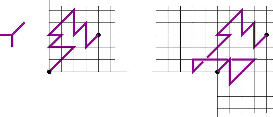
Figure 1: Two walks with Kreweras steps $\nearrow , \leftarrow , \downarrow $
, one in the first quadrant
$\nearrow , \leftarrow , \downarrow $
, one in the first quadrant $\mathcal {Q}$
(left), and one in the three-quadrant cone
$\mathcal {Q}$
(left), and one in the three-quadrant cone $\mathcal {C}$
(right). The associated generating functions are algebraic.
$\mathcal {C}$
(right). The associated generating functions are algebraic.
Using an asymptotic argument, Mustapha [Reference Mustapha28] quickly proved that the $51$
three-quadrant problems associated with an infinite group have, as their quadrant counterparts, a non-D-finite solution. Regarding exact solutions, Raschel and Trotignon obtained in [Reference Raschel and Trotignon31] sophisticated integral expressions for
$51$
three-quadrant problems associated with an infinite group have, as their quadrant counterparts, a non-D-finite solution. Regarding exact solutions, Raschel and Trotignon obtained in [Reference Raschel and Trotignon31] sophisticated integral expressions for $C(x,y;t)$
for the step sets
$C(x,y;t)$
for the step sets $\mathcal S$
of Table 1 (apart from the diagonal model). The first four have a finite group, and the expressions of [Reference Raschel and Trotignon31] imply that
$\mathcal S$
of Table 1 (apart from the diagonal model). The first four have a finite group, and the expressions of [Reference Raschel and Trotignon31] imply that $C(x,y;t)$
is indeed D-finite for these models (at least in x and y). The other four have an infinite group, and
$C(x,y;t)$
is indeed D-finite for these models (at least in x and y). The other four have an infinite group, and $C(x,y;t)$
is non-D-finite by [Reference Mustapha28]. These four non-D-finite models, labeled from
$C(x,y;t)$
is non-D-finite by [Reference Mustapha28]. These four non-D-finite models, labeled from $\#6$
to
$\#6$
to $\#9$
in Table 1, were further studied by Dreyfus and Trotignon [Reference Dreyfus and Trotignon17]: they proved that
$\#9$
in Table 1, were further studied by Dreyfus and Trotignon [Reference Dreyfus and Trotignon17]: they proved that $C(x,y;t)$
is D-algebraic for the first one (
$C(x,y;t)$
is D-algebraic for the first one ( $\#6$
), but not for the other three. More recently, the method used in the original paper [Reference Bousquet-Mélou9] was adapted to solve the so-called king model where all eight steps are allowed [Reference Bousquet-Mélou and Wallner11, Reference Bousquet-Mélou and Wallner12], again with a D-finite solution (and a finite group). Finally, remarkable results of Budd [Reference Budd13] and Elvey Price [Reference Elvey Price19] on the winding number of various families of plane walks provide explicit D-finite expressions for several series counting walks in
$\#6$
), but not for the other three. More recently, the method used in the original paper [Reference Bousquet-Mélou9] was adapted to solve the so-called king model where all eight steps are allowed [Reference Bousquet-Mélou and Wallner11, Reference Bousquet-Mélou and Wallner12], again with a D-finite solution (and a finite group). Finally, remarkable results of Budd [Reference Budd13] and Elvey Price [Reference Elvey Price19] on the winding number of various families of plane walks provide explicit D-finite expressions for several series counting walks in $\mathcal {C}$
with prescribed endpoints.
$\mathcal {C}$
with prescribed endpoints.
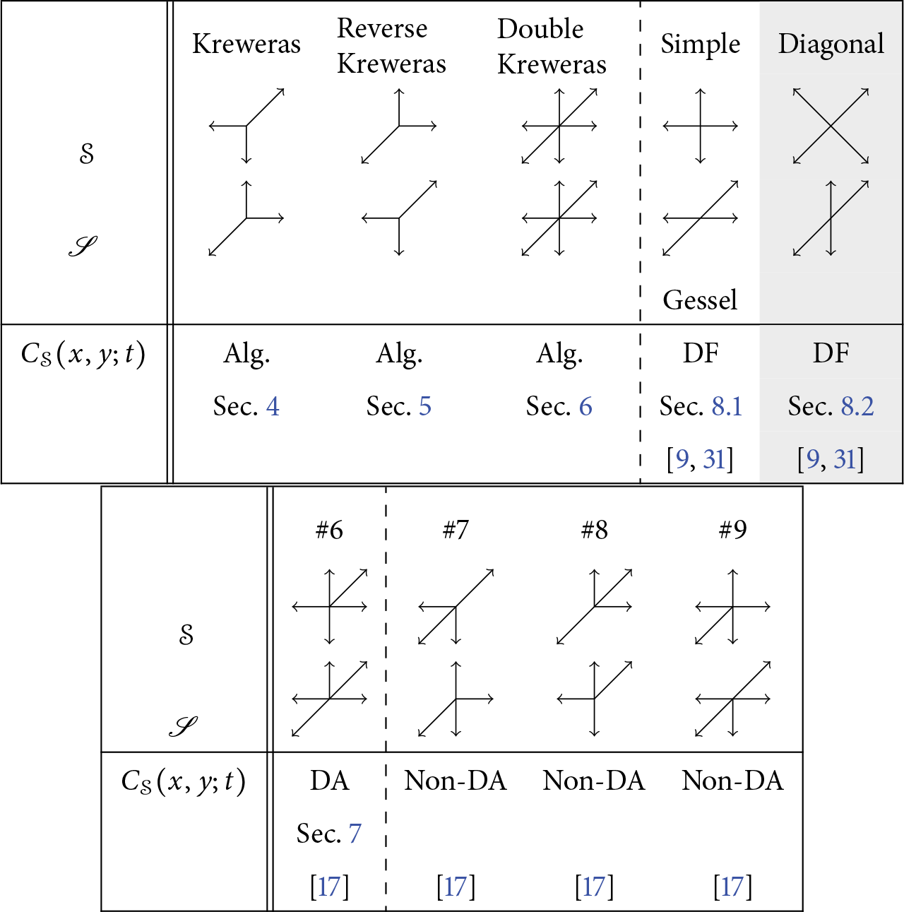
Table 1: The nine models $\mathcal S$
considered in this paper. One is the diagonal model (shaded column). The others are the eight models with
$\mathcal S$
considered in this paper. One is the diagonal model (shaded column). The others are the eight models with $x/y$
-symmetry and no step
$x/y$
-symmetry and no step $\nwarrow $
nor
$\nwarrow $
nor $\searrow $
. Each model is shown with its companion model
$\searrow $
. Each model is shown with its companion model $\mathscr S$
, with step polynomial
$\mathscr S$
, with step polynomial $S(1/x, xy)$
(or
$S(1/x, xy)$
(or $S(1/\sqrt x , \sqrt x y)$
for the diagonal model). The first five models have a finite group, and the other four an infinite group.
$S(1/\sqrt x , \sqrt x y)$
for the diagonal model). The first five models have a finite group, and the other four an infinite group.
1.3 Invariants
One of the many approaches that have been applied to quadrant walks relies on the notion of invariants, introduced by William Tutte in the seventies and eighties in his study of colored planar triangulations [Reference Tutte33]. These invariants come by pairs and consist of two series $I(x;t)$
and
$I(x;t)$
and $J(y;t)$
satisfying some properties (precise definitions will be given later). It follows from [Reference Bernardi, Bousquet-Mélou and Raschel2, Reference Bostan, Chyzak, van Hoeij, Kauers and Pech4, Reference Dreyfus, Hardouin, Roques and Singer15, Reference Dreyfus, Hardouin, Roques and Singer16, Reference Hardouin and Singer22] that invariants play a crucial role in the classification of quadrant models. In particular, it was first proved in [Reference Bernardi, Bousquet-Mélou and Raschel2] that:
$J(y;t)$
satisfying some properties (precise definitions will be given later). It follows from [Reference Bernardi, Bousquet-Mélou and Raschel2, Reference Bostan, Chyzak, van Hoeij, Kauers and Pech4, Reference Dreyfus, Hardouin, Roques and Singer15, Reference Dreyfus, Hardouin, Roques and Singer16, Reference Hardouin and Singer22] that invariants play a crucial role in the classification of quadrant models. In particular, it was first proved in [Reference Bernardi, Bousquet-Mélou and Raschel2] that:
-
• among the $79$
nontrivial quadrant models, exactly
$13$
admit invariants involving the series
$Q(x,y;t)$
: four of these models have a finite group and nine an infinite group;
$79$
nontrivial quadrant models, exactly
$13$
admit invariants involving the series
$Q(x,y;t)$
: four of these models have a finite group and nine an infinite group; -
• one can use these invariants to prove, in a uniform manner, that
$Q(x,y;t)$
is algebraic for the four models with a finite group (and invariants); -
• one can use these invariants to prove, in a uniform manner, that
$Q(x,y;t)$
is D-algebraic for the nine models with an infinite group (and invariants).


Moreover, it was already known at that time that the other $19$
models with a finite group are transcendental (i.e., not algebraic) [Reference Bostan, Chyzak, van Hoeij, Kauers and Pech4]. Hence, for finite group models, algebraicity is equivalent to the existence of invariants involving Q. Similarly, the D-algebraicity results for the nine infinite group models were complemented using differential Galois theory [Reference Dreyfus, Hardouin, Roques and Singer15, Reference Dreyfus, Hardouin, Roques and Singer16], proving that for infinite group models, D-algebraicity is equivalent to the existence of invariants involving Q. This equivalence has recently been generalized to quadrant walks with weighted steps (in the infinite group case) [Reference Hardouin and Singer22].
$19$
models with a finite group are transcendental (i.e., not algebraic) [Reference Bostan, Chyzak, van Hoeij, Kauers and Pech4]. Hence, for finite group models, algebraicity is equivalent to the existence of invariants involving Q. Similarly, the D-algebraicity results for the nine infinite group models were complemented using differential Galois theory [Reference Dreyfus, Hardouin, Roques and Singer15, Reference Dreyfus, Hardouin, Roques and Singer16], proving that for infinite group models, D-algebraicity is equivalent to the existence of invariants involving Q. This equivalence has recently been generalized to quadrant walks with weighted steps (in the infinite group case) [Reference Hardouin and Singer22].
1.4 Main results
The aim of this paper is to explore the applicability of invariants in the solution of three-quadrant models. We focus on the nine models of Table 1, because the series $C(x,y;t)$
can then be described by an equation that is reminiscent of a quadrant equation, although more complex. These models (apart from the diagonal one) are already those considered in [Reference Raschel and Trotignon31]. Our first contribution is, for this (admittedly small) set of models, a collection of results that are perfect analogues of the above quadrant results:
$C(x,y;t)$
can then be described by an equation that is reminiscent of a quadrant equation, although more complex. These models (apart from the diagonal one) are already those considered in [Reference Raschel and Trotignon31]. Our first contribution is, for this (admittedly small) set of models, a collection of results that are perfect analogues of the above quadrant results:
-
• Exactly four of these nine models admit invariants involving the series
$C(x,y;t)$
: three of them (those of the Kreweras trilogy on the left of the top table) have a finite group, and one (
$\#6$
) has an infinite group. Moreover, these four models are also those that admit invariants involving the series
$Q(x,y;t)$
(Proposition 3.1). -
• We use these invariants to prove, in a uniform manner, that the series
$C(x,y;t)$
is algebraic for the three models with a finite group (and invariants); this series was already known to be D-finite in x and y [Reference Raschel and Trotignon31], and conjectured to be algebraic [Reference Bousquet-Mélou9]. -
• We use these invariants to (re)prove that the series
$C(x,y;t)$
is D-algebraic for the (unique) model with an infinite group and invariants. This series was already known to be D-algebraic [Reference Dreyfus and Trotignon17], but the expression that we obtain is new.


As in the quadrant case, these “positive” results are complemented by “negative” ones from the existing literature, which imply a tight connection between invariants and (D)-algebraicity: the series $C(x,y;t)$
is transcendental for the fourth and fifth models with a finite group (simple walks and diagonal walks) [Reference Bousquet-Mélou9], and non-D-algebraic for the other three models with an infinite group [Reference Dreyfus and Trotignon17]. These properties are summarized in Table 1.
$C(x,y;t)$
is transcendental for the fourth and fifth models with a finite group (simple walks and diagonal walks) [Reference Bousquet-Mélou9], and non-D-algebraic for the other three models with an infinite group [Reference Dreyfus and Trotignon17]. These properties are summarized in Table 1.
Our second contribution is a new solution of two (transcendental) D-finite models via invariants: simple walks with steps $\rightarrow , \uparrow , \leftarrow , \downarrow $
and diagonal walks with steps
$\rightarrow , \uparrow , \leftarrow , \downarrow $
and diagonal walks with steps $\nearrow , \nwarrow , \swarrow , \searrow $
(fourth and fifth in the table). This may seem surprising, since, for finite group models, invariants have so far been used to prove algebraicity results. However, as shown in [Reference Bousquet-Mélou9] for both models, it is natural to introduce a series
$\nearrow , \nwarrow , \swarrow , \searrow $
(fourth and fifth in the table). This may seem surprising, since, for finite group models, invariants have so far been used to prove algebraicity results. However, as shown in [Reference Bousquet-Mélou9] for both models, it is natural to introduce a series $A(x,y;t)$
that differs from
$A(x,y;t)$
that differs from $C(x,y;t)$
by a simple explicit D-finite series (expressed in terms of
$C(x,y;t)$
by a simple explicit D-finite series (expressed in terms of $Q(x,y;t)$
), and then the heart of the solution of [Reference Bousquet-Mélou9] is to prove that
$Q(x,y;t)$
), and then the heart of the solution of [Reference Bousquet-Mélou9] is to prove that $A(x,y;t)$
is algebraic. What we show here is how to reprove this algebraicity via invariants.
$A(x,y;t)$
is algebraic. What we show here is how to reprove this algebraicity via invariants.
In the six cases that we solve via invariants (the first six in Table 1), what we actually establish is an algebraic relation between the three-quadrant series $C(x,y;t)$
(or
$C(x,y;t)$
(or $A(x,y;t)$
in the simple and diagonal cases) for the model
$A(x,y;t)$
in the simple and diagonal cases) for the model $\mathcal S$
, and the quadrant series
$\mathcal S$
, and the quadrant series $\mathscr Q(x,y;t)$
for a companion model
$\mathscr Q(x,y;t)$
for a companion model $\mathscr S$
also shown in Table 1. The (D)-algebraicity of
$\mathscr S$
also shown in Table 1. The (D)-algebraicity of $C(x,y;t)$
(or
$C(x,y;t)$
(or $A(x,y;t)$
) then follows from the (D)-algebraicity of
$A(x,y;t)$
) then follows from the (D)-algebraicity of $\mathscr Q(x,y;t)$
. (Note that
$\mathscr Q(x,y;t)$
. (Note that $\mathscr Q(x,y;t)$
is also D-algebraic for the three models that we do not solve, but the lack of invariants involving
$\mathscr Q(x,y;t)$
is also D-algebraic for the three models that we do not solve, but the lack of invariants involving $C(x,y;t)$
prevents us from relating
$C(x,y;t)$
prevents us from relating $C(x,y;t)$
and
$C(x,y;t)$
and $\mathscr Q(x,y;t)$
.) We thus obtain either explicit algebraic expressions of
$\mathscr Q(x,y;t)$
.) We thus obtain either explicit algebraic expressions of $C(x,y;t)$
or
$C(x,y;t)$
or $A(x,y;t)$
, or, for the model that is only D-algebraic, an expression in terms of the weak invariant of [Reference Bostan, Bousquet-Mélou and Melczer3].
$A(x,y;t)$
, or, for the model that is only D-algebraic, an expression in terms of the weak invariant of [Reference Bostan, Bousquet-Mélou and Melczer3].
Finally, for the five models $\mathcal S$
that are (at least) D-finite, we derive from our results explicit algebraic expressions for the series
$\mathcal S$
that are (at least) D-finite, we derive from our results explicit algebraic expressions for the series $\sum _{i,j} H_{i,j} x^i y^j$
, where
$\sum _{i,j} H_{i,j} x^i y^j$
, where $\left (H_{i,j}\right ) _{(i,j)\in \mathcal {C}}$
is a discrete positive harmonic function in
$\left (H_{i,j}\right ) _{(i,j)\in \mathcal {C}}$
is a discrete positive harmonic function in $\mathcal {C}$
associated with the reverse set of steps,
$\mathcal {C}$
associated with the reverse set of steps, $\mathcal S^*:=\{(-i,-j): (i,j)\in \mathcal S\}$
. It is widely believed that there exists a unique such function, up to a multiplicative constant. As can now be expected, the above series is related to the series describing the/a harmonic function associated with the step set
$\mathcal S^*:=\{(-i,-j): (i,j)\in \mathcal S\}$
. It is widely believed that there exists a unique such function, up to a multiplicative constant. As can now be expected, the above series is related to the series describing the/a harmonic function associated with the step set $\mathscr S^*$
in the quadrant. We prove that this relation still holds, under natural assumptions, for the sixth model that we solve.
$\mathscr S^*$
in the quadrant. We prove that this relation still holds, under natural assumptions, for the sixth model that we solve.
1.5 Outline of the paper
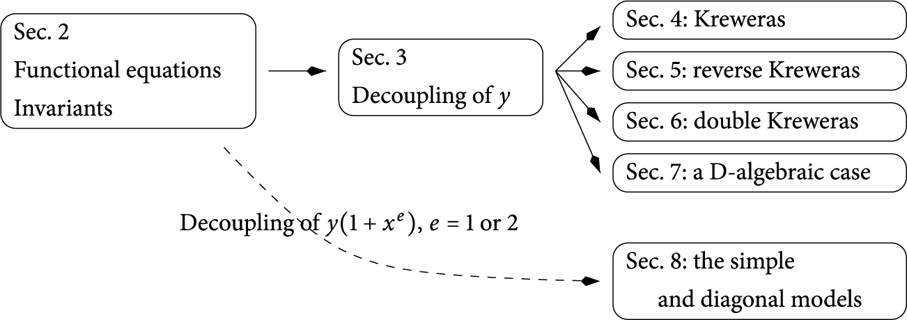
The paper is organized as follows. In Section 2, we introduce general tools, like basic functional equations for walks in $\mathcal {C}$
, and also the key notion of pairs of invariants. For each of the models
$\mathcal {C}$
, and also the key notion of pairs of invariants. For each of the models $\mathscr S$
of Table 1, we give one or two pairs of
$\mathscr S$
of Table 1, we give one or two pairs of $\mathscr S$
-invariants, borrowed from [Reference Bernardi, Bousquet-Mélou and Raschel2]: one pair involves the generating function
$\mathscr S$
-invariants, borrowed from [Reference Bernardi, Bousquet-Mélou and Raschel2]: one pair involves the generating function $\mathscr Q(x,y;t)$
of quadrant walks with steps in
$\mathscr Q(x,y;t)$
of quadrant walks with steps in $\mathscr S$
, and the other one, which only exists for finite group models, is rational. In Section 3, we construct, for models of the Kreweras trilogy and for the
$\mathscr S$
, and the other one, which only exists for finite group models, is rational. In Section 3, we construct, for models of the Kreweras trilogy and for the $6$
th model of the table, a new pair of
$6$
th model of the table, a new pair of $\mathscr S$
-invariants involving the generating function of walks in
$\mathscr S$
-invariants involving the generating function of walks in $\mathcal {C}$
with steps in
$\mathcal {C}$
with steps in $\mathcal S$
(note the change in the step set). This construction is based on a certain decoupling property in these models, which we relate to the decoupling property used in the solution of quadrant walks with steps in
$\mathcal S$
(note the change in the step set). This construction is based on a certain decoupling property in these models, which we relate to the decoupling property used in the solution of quadrant walks with steps in $\mathcal S$
by invariants (Proposition 3.1). A basic, but useful, invariant lemma (Lemma 2.6) allows us to relate these new invariants to the known ones. This connection is made explicit in Sections 4–7 for Kreweras steps, reverse Kreweras steps, double Kreweras steps, and for the
$\mathcal S$
by invariants (Proposition 3.1). A basic, but useful, invariant lemma (Lemma 2.6) allows us to relate these new invariants to the known ones. This connection is made explicit in Sections 4–7 for Kreweras steps, reverse Kreweras steps, double Kreweras steps, and for the $6$
th model of Table 1, respectively. We thus relate the generating function
$6$
th model of Table 1, respectively. We thus relate the generating function $C(x,y;t)$
for three-quadrant
$C(x,y;t)$
for three-quadrant $\mathcal S$
-walks to the generating function
$\mathcal S$
-walks to the generating function $\mathscr Q(x,y;t)$
for quadrant
$\mathscr Q(x,y;t)$
for quadrant $\mathscr S$
-walks. In Section 8, we apply the same approach to solve the simple and diagonal models, proving that the series
$\mathscr S$
-walks. In Section 8, we apply the same approach to solve the simple and diagonal models, proving that the series $A(x,y;t)$
is algebraic in both cases. We finish in Section 9 with comments and perspectives.
$A(x,y;t)$
is algebraic in both cases. We finish in Section 9 with comments and perspectives.
The paper is accompanied by six Maple sessions (one per step set) available on the author’s web page (http://www.labri.fr/perso/bousquet/publis.html).
1.6 Kreweras’ model
To illustrate our results, we now present those that deal with Kreweras’ model, $\mathcal S=\{\nearrow , \leftarrow , \downarrow \}$
. Note that we often omit the dependency in t of our series, denoting, for instance,
$\mathcal S=\{\nearrow , \leftarrow , \downarrow \}$
. Note that we often omit the dependency in t of our series, denoting, for instance, $C(x,y)$
for
$C(x,y)$
for $C(x,y;t)$
. We also use the notation
$C(x,y;t)$
. We also use the notation $\bar x=1/x$
and
$\bar x=1/x$
and $\bar y=1/y$
.
$\bar y=1/y$
.
Theorem 1.1 The generating function $C(x,y)$
of walks with steps in
$C(x,y)$
of walks with steps in $\{\nearrow , \leftarrow , \downarrow \}$
starting from
$\{\nearrow , \leftarrow , \downarrow \}$
starting from $(0,0)$
and avoiding the negative quadrant is algebraic of degree
$(0,0)$
and avoiding the negative quadrant is algebraic of degree $96$
. It is given by the following identity:
$96$
. It is given by the following identity:
 $$\begin{align*}(1-t(\bar x+\bar y +xy)) C(x,y)=1 -t\bar y C_-(\bar x) -t\bar x C_-(\bar y), \end{align*}$$
where $C_-(x)$
is a series in t with polynomial coefficients in x, algebraic of degree
$C_-(x)$
is a series in t with polynomial coefficients in x, algebraic of degree $24$
. This series can be expressed explicitly in terms of the unique formal power series
$24$
. This series can be expressed explicitly in terms of the unique formal power series $V\equiv V(t)$
satisfying
$V\equiv V(t)$
satisfying
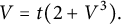 $$ \begin{align} V=t(2+V^3).\\[-9pt]\nonumber \end{align} $$
Indeed,
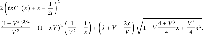 $$ \begin{align*} &2\left(t\bar x C_-(x)+ x - \frac 1 {2t}\right)^2=\\ &\frac{ (1-V^3)^{3/2}}{V^2}+ (1-xV)^2 \left(\frac 1 {V^2}-\frac 1 x\right) + \left(\bar x +V-\frac{2x}V\right) \sqrt{1-V\frac{4+V^3}4 x+\frac{ V^2} 4 x^2}.\\[-9pt] \end{align*} $$
One recognizes, as announced, some ingredients of the quadrant generating function for the companion model $\mathscr S=\{\rightarrow , \uparrow , \swarrow \}$
, which satisfies [Reference Bousquet-Mélou and Mishna10, Reference Mishna26]
$\mathscr S=\{\rightarrow , \uparrow , \swarrow \}$
, which satisfies [Reference Bousquet-Mélou and Mishna10, Reference Mishna26]
 $$ \begin{align} \mathscr Q(x,0)=\frac{V(4-V^3)}{16t} - \frac{t-x^2+tx^3}{2xt^2}+ \left(\bar x +V-\frac{2x}V\right) \sqrt{1-V\frac{4+V^3}4 x+\frac{ V^2} 4 x^2}.\\[-9pt]\nonumber \end{align} $$
Note, however, that $\mathscr Q(x,0)$
has degree
$\mathscr Q(x,0)$
has degree $6$
only.
$6$
only.
We can complement Theorem 1.1 with the following one, which counts walks in $\mathcal {C}$
ending on the diagonal: as before, the variable t records the length, and the variable x the abscissa of the endpoint. Note that the expressions in the two theorems only differ by a sign in front of the square root.
$\mathcal {C}$
ending on the diagonal: as before, the variable t records the length, and the variable x the abscissa of the endpoint. Note that the expressions in the two theorems only differ by a sign in front of the square root.
Theorem 1.2 The generating function $D(x)$
of walks with steps in
$D(x)$
of walks with steps in $\{\nearrow , \leftarrow , \downarrow \}$
starting from
$\{\nearrow , \leftarrow , \downarrow \}$
starting from $(0,0)$
, avoiding the negative quadrant, and ending on the first diagonal is algebraic of degree
$(0,0)$
, avoiding the negative quadrant, and ending on the first diagonal is algebraic of degree $24$
. It can be written explicitly in terms of the series V defined by (1.3):
$24$
. It can be written explicitly in terms of the series V defined by (1.3):
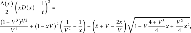 $$ \begin{align*} &\frac{\Delta(x)}2\left(xD(x)+ \frac 1 {t}\right)^2=\\ &\frac{ (1-V^3)^{3/2}}{V^2}+ (1-xV)^2 \left(\frac 1 {V^2}-\frac 1 x\right) - \left(\bar x +V-\frac{2x}V\right) \sqrt{1-V\frac{4+V^3}4 x+\frac{ V^2} 4 x^2},\\[-9pt] \end{align*} $$
where $ \Delta (x)= (1-tx)^2-4t^2\bar x$
.
$ \Delta (x)= (1-tx)^2-4t^2\bar x$
.
The generating function of excursions (that is, walks ending at $(0,0)$
) was conjectured in [Reference Bousquet-Mélou9] to be algebraic of degree
$(0,0)$
) was conjectured in [Reference Bousquet-Mélou9] to be algebraic of degree $6$
. More generally, it is natural to ask about the generating function
$6$
. More generally, it is natural to ask about the generating function $C_{i,j}$
of walks ending at a specific point
$C_{i,j}$
of walks ending at a specific point $(i,j)$
. In order to describe these series, we introduce an extension of degree
$(i,j)$
. In order to describe these series, we introduce an extension of degree $4$
of
$4$
of $\mathbb {Q}(V)$
(hence of degree
$\mathbb {Q}(V)$
(hence of degree $12$
over
$12$
over $\mathbb {Q}(t)$
). First, due to the periodicity of the model (walks ending at position
$\mathbb {Q}(t)$
). First, due to the periodicity of the model (walks ending at position $(i,j)$
have length
$(i,j)$
have length $-i-j$
modulo
$-i-j$
modulo $3$
), it makes sense to consider
$3$
), it makes sense to consider $t^3$
as the natural variable for this problem. Note that
$t^3$
as the natural variable for this problem. Note that
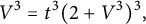 $$\begin{align*}V^3=t^3(2+V^3)^3, \end{align*}$$
so that all series in $t^3$
can be written as series in
$t^3$
can be written as series in $V^3$
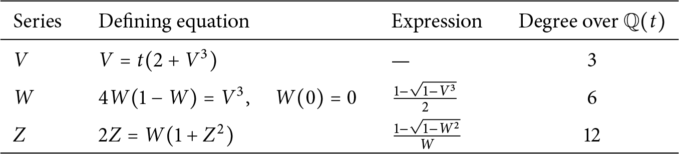
. We then define the series W and Z as described in Table 2. Both are formal power series in
$V^3$
. We then define the series W and Z as described in Table 2. Both are formal power series in $t^3$
, and we have the following tower of extensions:
$t^3$
, and we have the following tower of extensions:
 $$\begin{align*}\mathbb{Q}(t^3) \stackrel{3}{\hookrightarrow} \mathbb{Q}(V^3) \stackrel{2}{\hookrightarrow} \mathbb{Q}(W) \stackrel{2}{\hookrightarrow} \mathbb{Q}(Z). \end{align*}$$
Table 2: Relevant extensions of $\mathbb {Q}(t)$
for Kreweras (and reverse Kreweras) steps.
$\mathbb {Q}(t)$
for Kreweras (and reverse Kreweras) steps.
Corollary 1.3 Let us define $V, W $
, and Z as above. For any
$V, W $
, and Z as above. For any $(i,j) \in \mathcal {C}$
, the generating function
$(i,j) \in \mathcal {C}$
, the generating function $C_{i,j}$
of walks avoiding the negative quadrant and ending at
$C_{i,j}$
of walks avoiding the negative quadrant and ending at $(i,j)$
is algebraic of degree (at most)
$(i,j)$
is algebraic of degree (at most) $12$
, and belongs to
$12$
, and belongs to $\mathbb {Q}(t, Z)$
. More precisely,
$\mathbb {Q}(t, Z)$
. More precisely, $t^{i+j}C_{i,j}$
belongs to
$t^{i+j}C_{i,j}$
belongs to $\mathbb {Q}(Z)$
. If
$\mathbb {Q}(Z)$
. If $i=j$
or
$i=j$
or $i=j\pm 1$
with
$i=j\pm 1$
with $i,j\ge 0$
, then
$i,j\ge 0$
, then $t^{i+j}C_{i,j}$
has degree
$t^{i+j}C_{i,j}$
has degree $6$
at most and belongs to
$6$
at most and belongs to $\mathbb {Q}(W)$
.
$\mathbb {Q}(W)$
.
For instance, we have
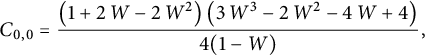 $$ \begin{align} C_{0,0}&={\frac { \left(1+2\,W- 2\,{W}^{2} \right) \left( 3\,{W}^{3}-2\,{W}^{2}-4\,W+4 \right) }{4(1-W)}}, \end{align} $$
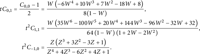 $$ \begin{align} tC_{0,1} = \frac {C_{0,0}-1} {2} & = {\frac {W \left( -6 {W}^{4}+10 {W}^{3}+7 {W}^{2}-18 W+8 \right) }{8(1-W)}}, \nonumber \\ t^2 C_{1,1}&= {\frac { W\left( 35 {W}^{6}-100 {W}^{5}+20 {W}^{4}+144 {W}^{3 }-96 {W}^{2}-32 W+32 \right) }{ 64\left(1- W \right) \left(1+2 W- 2 {W}^{2} \right) }}, \nonumber \\ t^2 C_{-1,0}&= {\frac {Z \left( {Z}^{3}+3 {Z}^{2}-3 Z+1 \right) }{ {Z}^{4}+4 {Z}^{3}-6 {Z}^{2}+4 Z+1 }}. \end{align} $$
We can derive from such results asymptotic estimates for the number of walks ending at $(i,j)$
via singularity analysis [Reference Flajolet and Sedgewick21, Chapter VII.7]. For instance,
$(i,j)$
via singularity analysis [Reference Flajolet and Sedgewick21, Chapter VII.7]. For instance,
 $$\begin{align*}c_{0,0}(3m) \sim -\frac{27\sqrt 3}{4\Gamma(-3/4)} 3^{3m} (3m)^{-7/4}. \end{align*}$$
Note that this asymptotic behavior was already known, but only up to a constant [Reference Mustapha28]. More generally, we obtain an explicit description of a discrete positive harmonic function associated with $\mathcal S^*$
-walks in the three-quadrant cone
$\mathcal S^*$
-walks in the three-quadrant cone $\mathcal C$
, where we recall that
$\mathcal C$
, where we recall that $\mathcal S^*=\{(-i,-j), (i,j)\in \mathcal S\}$
.
$\mathcal S^*=\{(-i,-j), (i,j)\in \mathcal S\}$
.
Corollary 1.4 For $(i,j)\in \mathcal C$
, there exists a positive constant
$(i,j)\in \mathcal C$
, there exists a positive constant $H_{i,j}$
such that, as
$H_{i,j}$
such that, as $n\rightarrow \infty $
with
$n\rightarrow \infty $
with $n+i+j \equiv 0\ \mod 3$
,
$n+i+j \equiv 0\ \mod 3$
,
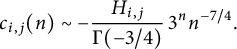 $$ \begin{align} c_{i,j}(n) \sim -\frac{H_{i,j}}{\Gamma(-3/4)}\, 3^n n^{-7/4}. \end{align} $$
The function H is discrete harmonic for the step set $\mathcal S^*=\{\swarrow , \rightarrow , \uparrow \}$
. That is,
$\mathcal S^*=\{\swarrow , \rightarrow , \uparrow \}$
. That is,
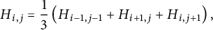 $$ \begin{align} H_{i,j} = \frac 1 3 \left( H_{i-1,j-1}+ H_{i+1,j} + H_{i,j+1}\right), \end{align} $$
where $H_{i,j}=0$
if
$H_{i,j}=0$
if $(i,j) \not \in \mathcal C$
. By symmetry,
$(i,j) \not \in \mathcal C$
. By symmetry, $H_{i,j}=H_{j,i}$
. The generating function
$H_{i,j}=H_{j,i}$
. The generating function
 $$ \begin{align} \mathcal H(x,y):=\sum_{j\ge 0, i\le j} H_{i,j} x^{j-i} y^j, \end{align} $$
which is a formal power series in x and y, is algebraic of degree $16$
, given by
$16$
, given by
 $$ \begin{align} \qquad \left(1+xy^2+x^2y-3xy\right) \mathcal H(x,y)= \mathcal H_-(x)+\frac 1 2 \left(2+xy^2-3xy\right) \mathcal H_d(y), \end{align} $$
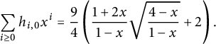
where
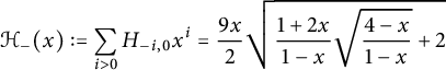 $$ \begin{align} \mathcal H_-(x):=\sum_{i>0} H_{-i,0} x^i=\frac {9x}{2} \sqrt{ \frac{1+2x}{1-x} \sqrt{\frac {4-x}{1-x}}+2} \end{align} $$
and
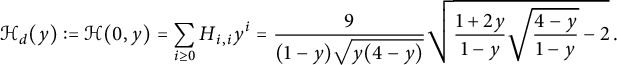 $$ \begin{align} \qquad \mathcal H_d(y):=\mathcal H(0,y)=\sum_{i\ge 0} H_{i,i}y^i = \frac 9 { (1-y) \sqrt{y(4-y)}}\sqrt{ \frac{1+2y}{1-y} \sqrt{\frac {4-y}{1-y}}-2}\,. \end{align} $$
Remark 1.5 It may seem surprising to read that we derive, from the asymptotic enumeration of $\mathcal S$
-walks in
$\mathcal S$
-walks in $\mathcal {C}$
, the expression of a function H that is
$\mathcal {C}$
, the expression of a function H that is $\mathcal S^*$
-harmonic, rather than
$\mathcal S^*$
-harmonic, rather than $\mathcal S$
-harmonic. This is simply due to the definition of discrete harmonic functions (e.g., [Reference Raschel30]): a function
$\mathcal S$
-harmonic. This is simply due to the definition of discrete harmonic functions (e.g., [Reference Raschel30]): a function $f_{i,j}$
is harmonic for the (uniform) random walk with steps in
$f_{i,j}$
is harmonic for the (uniform) random walk with steps in $\mathcal P$
if
$\mathcal P$
if
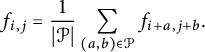 $$\begin{align*}f_{i,j}= \frac 1 {|\mathcal P|} \sum_{(a,b)\in \mathcal P} f_{i+a,j+b}. \end{align*}$$
A $\mathcal P$
-harmonic function typically occurs in the asymptotic enumeration of
$\mathcal P$
-harmonic function typically occurs in the asymptotic enumeration of $\mathcal P$
-walks starting (rather than ending) at
$\mathcal P$
-walks starting (rather than ending) at $(i,j)$
. In many cases, this number behaves like
$(i,j)$
. In many cases, this number behaves like $f_{i,j} \mu ^n n^\gamma $
, for constants
$f_{i,j} \mu ^n n^\gamma $
, for constants $\mu $
and
$\mu $
and $\gamma $
, where the function f is
$\gamma $
, where the function f is $\mathcal P$
-harmonic. As already mentioned, it is widely believed (and proved in some cases [Reference Bouaziz, Mustapha and Sifi7, Reference Duraj, Raschel, Tarrago and Wachtel18, Reference Ignatiouk-Robert23, Reference Mustapha and Sifi29]) that for many domains
$\mathcal P$
-harmonic. As already mentioned, it is widely believed (and proved in some cases [Reference Bouaziz, Mustapha and Sifi7, Reference Duraj, Raschel, Tarrago and Wachtel18, Reference Ignatiouk-Robert23, Reference Mustapha and Sifi29]) that for many domains $\mathcal D$
and step sets with zero drift, there exists (up to a multiplicative constant) a unique positive harmonic function in
$\mathcal D$
and step sets with zero drift, there exists (up to a multiplicative constant) a unique positive harmonic function in $\mathcal D$
that vanishes at the boundary.
$\mathcal D$
that vanishes at the boundary.
The first expression of a/the harmonic function, implying its algebraicity, was given by Trotignon [Reference Trotignon32]. It is, however, less explicit than in Corollary 1.4. The connection between walks in $\mathcal C$
with steps in
$\mathcal C$
with steps in $\mathcal S$
and walks in
$\mathcal S$
and walks in $\mathcal {Q}$
with steps in the companion model
$\mathcal {Q}$
with steps in the companion model $\mathscr S$
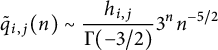
, already observed at the level of generating functions (see Theorem 1.1 and (1.4)), is also visible at the level of harmonic functions. Indeed, the number of quadrant
$\mathscr S$
, already observed at the level of generating functions (see Theorem 1.1 and (1.4)), is also visible at the level of harmonic functions. Indeed, the number of quadrant $\mathscr S$
-walks of length n ending at
$\mathscr S$
-walks of length n ending at $(i,j)\in \mathcal {Q}$
is
$(i,j)\in \mathcal {Q}$
is
 $$ \begin{align} \tilde q_{i,j}(n) \sim \frac{h_{i,j} }{\Gamma(-3/2)} 3^n n^{-5/2} \end{align} $$
(for $n\equiv i+j $
mod
$n\equiv i+j $
mod $3$
) with
$3$
) with
 $$ \begin{align} \sum_{i\ge0} h_{i,0} x^i= \frac 9 4 \left( \frac{1+2x}{1-x} \sqrt{\frac{4-x}{1-x}}+2\right). \end{align} $$
This should be compared to (1.11) and (1.12). This expression can be derived from (1.4) by singularity analysis. See also [Reference Raschel30] for a more general expression that applies to any quadrant model with small steps and zero drift. We explain in Remark 4.1 how one can predict, under a natural assumption, the relation between the $\mathcal S^*$
-harmonic function
$\mathcal S^*$
-harmonic function $H_{i,j}$
in
$H_{i,j}$
in $\mathcal C$
and the
$\mathcal C$
and the $\mathscr S^*$
-harmonic function
$\mathscr S^*$
-harmonic function $h_{i,j}$
in
$h_{i,j}$
in $\mathcal {Q}$
. Note that (1.13) also describes the asymptotic number of walks with steps in the original model
$\mathcal {Q}$
. Note that (1.13) also describes the asymptotic number of walks with steps in the original model $\mathcal S$
confined to the nonpositive quadrant, joining
$\mathcal S$
confined to the nonpositive quadrant, joining $(0,0)$
to
$(0,0)$
to $(-i,-j)$
.
$(-i,-j)$
.
Let us finally consider the total number of n-step walks avoiding the negative quadrant, which we denote by $c_n$
.
$c_n$
.
Corollary 1.6 The generating function $C(1,1)$
counting all walks confined to the three-quadrant cone
$C(1,1)$
counting all walks confined to the three-quadrant cone $\mathcal {C}$
is algebraic of degree
$\mathcal {C}$
is algebraic of degree $24$
, and given by
$24$
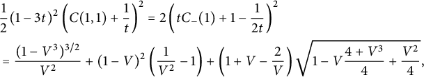
, and given by
 $$ \begin{align} \qquad &\frac 1 2 (1-3t)^2\left( C(1,1)+\frac 1 t\right)^2 = 2\left(t C_-(1)+ 1 - \frac 1 {2t}\right)^2 \nonumber \\ &= \frac{ (1-V^3)^{3/2}}{V^2}+ (1-V)^2 \left(\frac 1 {V^2}-1\right) + \left(1+V-\frac{2}V\right) \sqrt{1-V\frac{4+V^3}4 +\frac{ V^2} 4 }, \end{align} $$
where V is the series defined by (1.3). The series $C(1,1)$
has radius of convergence
$C(1,1)$
has radius of convergence $1/3$
, with dominant singularities at
$1/3$
, with dominant singularities at $\zeta /3$
, where
$\zeta /3$
, where $\zeta $
is any cubic root of unity. For the first-order asymptotics of the coefficients
$\zeta $
is any cubic root of unity. For the first-order asymptotics of the coefficients $c_n$
, only the singularity at
$c_n$
, only the singularity at $1/3$
contributes, and
$1/3$
contributes, and
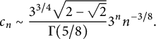 $$ \begin{align} c_n \sim \frac{3^{3/4}\sqrt{2-\sqrt 2}}{\Gamma(5/8)} 3^{n} n^{-3/8}. \end{align} $$
2 General tools
We first introduce some basic notation. For a ring R, we denote by $R[t]$
(resp.
$R[t]$
(resp. $R[[t]]$
) the ring of polynomials (resp. formal power series) in t with coefficients in R. If R is a field, then
$R[[t]]$
) the ring of polynomials (resp. formal power series) in t with coefficients in R. If R is a field, then $R(t)$
stands for the field of rational functions in t, and
$R(t)$
stands for the field of rational functions in t, and $R((t))$
for the field of Laurent series in t, that is, series of the form
$R((t))$
for the field of Laurent series in t, that is, series of the form $ \sum _{n \ge n_0} a_n t^n, $
with
$ \sum _{n \ge n_0} a_n t^n, $
with $n_0\in \mathbb {Z}$
and
$n_0\in \mathbb {Z}$
and $a_n\in R$
. This notation is generalized to several variables. For instance, the generating function
$a_n\in R$
. This notation is generalized to several variables. For instance, the generating function $C(x,y;t)$
of walks confined to
$C(x,y;t)$
of walks confined to $\mathcal C$
belongs to
$\mathcal C$
belongs to $\mathbb {Q}[x,\bar x,y,\bar y ][[t]]$
, where we denote
$\mathbb {Q}[x,\bar x,y,\bar y ][[t]]$
, where we denote $\bar x=1/x$
and
$\bar x=1/x$
and $\bar y=1/y$
. We often omit in our notation the dependency in t of our series, writing, for instance,
$\bar y=1/y$
. We often omit in our notation the dependency in t of our series, writing, for instance, $C(x,y)$
instead of
$C(x,y)$
instead of $C(x,y;t)$
. For a series
$C(x,y;t)$
. For a series $F(x,y) \in \mathbb {Q}[x, \bar x, y, \bar y][[t]]$
and two integers i and j, we denote by
$F(x,y) \in \mathbb {Q}[x, \bar x, y, \bar y][[t]]$
and two integers i and j, we denote by $F_{i,j}$
the coefficient of
$F_{i,j}$
the coefficient of $x^i y^j$
in
$x^i y^j$
in $F(x,y)$
. This is a series in
$F(x,y)$
. This is a series in $\mathbb {Q}[[t]]$
. Similarly, if
$\mathbb {Q}[[t]]$
. Similarly, if $F(x) \in \mathbb {Q}[x, \bar x][[t]]$
, then
$F(x) \in \mathbb {Q}[x, \bar x][[t]]$
, then $F_{i}$
stands for the coefficient of
$F_{i}$
stands for the coefficient of $x^i$
in
$x^i$
in $F(x)$
.
$F(x)$
.
We consider a set of “small” steps $\mathcal S$
in
$\mathcal S$
in $\mathbb {Z}^2$
, meaning that
$\mathbb {Z}^2$
, meaning that $\mathcal S\subset \{-1, 0, 1\}^2\setminus \{(0,0)\}$
. We define the step polynomial
$\mathcal S\subset \{-1, 0, 1\}^2\setminus \{(0,0)\}$
. We define the step polynomial $S(x,y)$
by
$S(x,y)$
by
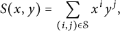 $$\begin{align*}S(x,y)=\sum_{(i,j)\in \mathcal S} x^i y^j, \end{align*}$$
and six (Laurent) polynomials $H_0$
,
$H_0$
, $H_-$
,
$H_-$
, $H_+$
,
$H_+$
, $V_0$
,
$V_0$
, $V_-$
, and
$V_-$
, and $V_+$
by
$V_+$
by
 $$ \begin{align} \qquad S(x,y)= \bar y H_-(x)+ H_0(x)+yH_+(x) = \bar x V_-(y) + V_0(y) + xV_+(y). \end{align} $$
The notation H (resp. V) recalls that these polynomials record horizontal (resp. vertical) moves: for instance, $H_-(x)$
describes the horizontal displacements of steps that move down. The group associated with
$H_-(x)$
describes the horizontal displacements of steps that move down. The group associated with $\mathcal S$
can be easily defined at this stage, but we do not use it in this paper, and simply refer the interested reader to, e.g., [Reference Bousquet-Mélou and Mishna10].
$\mathcal S$
can be easily defined at this stage, but we do not use it in this paper, and simply refer the interested reader to, e.g., [Reference Bousquet-Mélou and Mishna10].
2.1 Functional equations for walks avoiding a quadrant
In this subsection, we first restrict our attention to step sets $\mathcal S$
satisfying the following two assumptions:
$\mathcal S$
satisfying the following two assumptions:
This corresponds to the models shown in Table 1, apart from the diagonal model. As we shall explain, the latter model should still be considered in the same class, as the associated generating function satisfies the same kind of functional equation.
It is easy to write a functional equation defining the series
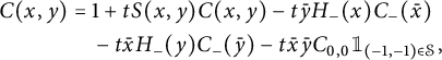
 $C(x,y)$
, based on a step-by-step construction of the walks:
$C(x,y)$
, based on a step-by-step construction of the walks:
where the series $C_{-}(\bar x)$
counts walks ending on the negative x-axis:
$C_{-}(\bar x)$
counts walks ending on the negative x-axis:
 $$ \begin{align} C_{-}(\bar x) = \sum_{i<0, n \geq 0} c_{i,0}(n)x^i t^n. \end{align} $$
In the above functional equation, each term with a minus sign corresponds to a forbidden move: moving down from the negative x-axis, moving left from the negative y-axis, or performing a South-West step from the point $(0,0)$
. Observe that we have exploited the
$(0,0)$
. Observe that we have exploited the $x/y$
-symmetry of
$x/y$
-symmetry of $\mathcal S$
. The above equation rewrites as
$\mathcal S$
. The above equation rewrites as
where $K(x,y):=1-tS(x,y)$
is the kernel of the equation.
$K(x,y):=1-tS(x,y)$
is the kernel of the equation.
Following [Reference Raschel and Trotignon31], we will now work in convex cones by splitting the three-quadrant cone in two symmetric halves. The rest of this subsection simply rephrases Section 2.2 of [Reference Raschel and Trotignon31], with a slightly different presentation. (Another strategy, namely splitting in three quadrants, is applied in [Reference Bousquet-Mélou9, Reference Bousquet-Mélou and Wallner11, Reference Bousquet-Mélou and Wallner12, Reference Elvey Price20].) We write
 $$ \begin{align} C(x,y)=\bar x U(\bar x, xy)+ D(xy)+ \bar y U(\bar y,xy), \end{align} $$
with $D(y) \in \mathbb {Q}[y][[t]]$
and
$D(y) \in \mathbb {Q}[y][[t]]$
and $U(x,y) \in \mathbb {Q} [x,y][[t]]$
. Observe that these properties, together with the above identity, define the series D and U uniquely: the series
$U(x,y) \in \mathbb {Q} [x,y][[t]]$
. Observe that these properties, together with the above identity, define the series D and U uniquely: the series $\bar x U(\bar x, xy)$
(resp.
$\bar x U(\bar x, xy)$
(resp. $D(xy)$
,
$D(xy)$
, $\bar y U(\bar y,xy)$
) counts walks ending strictly above (resp. on, strictly below) the diagonal (see Figure 2). We will now write functional equations for U and D, based again on a step-by-step construction (we could also derive them algebraically from (2.4), but we prefer a combinatorial argument). This requires to classify steps of
$\bar y U(\bar y,xy)$
) counts walks ending strictly above (resp. on, strictly below) the diagonal (see Figure 2). We will now write functional equations for U and D, based again on a step-by-step construction (we could also derive them algebraically from (2.4), but we prefer a combinatorial argument). This requires to classify steps of $\mathcal S$
according to whether they lie above, on or below the main diagonal. We write accordingly
$\mathcal S$
according to whether they lie above, on or below the main diagonal. We write accordingly
 $$ \begin{align} S(x,y)=\bar x\, \mathscr V_+(xy) + \mathscr V_0(xy) +x \mathscr V_-(xy). \end{align} $$
Note that this is only possible because we have forbidden steps $(1,-1)$
and
$(1,-1)$
and $(-1,1)$
, which would contribute terms of the form
$(-1,1)$
, which would contribute terms of the form $x^2 (\bar x\bar y)$
and
$x^2 (\bar x\bar y)$
and $\bar x^2 (xy)$
, respectively. Let us explain the notation
$\bar x^2 (xy)$
, respectively. Let us explain the notation $\mathscr V_+, \mathscr V_0, \mathscr V_-$
, which is reminiscent of (2.1). We define the companion set of steps
$\mathscr V_+, \mathscr V_0, \mathscr V_-$
, which is reminiscent of (2.1). We define the companion set of steps
 $$ \begin{align} \mathscr S:= \{(j-i,j): (i,j) \in \mathcal S\}, \end{align} $$
with step polynomial $\mathscr S(x,y)= S(\bar x,xy)$
(we hope that using the same notation
$\mathscr S(x,y)= S(\bar x,xy)$
(we hope that using the same notation $\mathscr S$
for the set of steps and its generating polynomial will not cause any inconvenience). Then
$\mathscr S$
for the set of steps and its generating polynomial will not cause any inconvenience). Then
 $$\begin{align*}\mathscr S(x,y)= S(\bar x, xy)= x\mathscr V_+(y) + \mathscr V_0(y) + \bar x\,\mathscr V_-(y), \end{align*}$$
which is indeed the decomposition of $\mathscr S$
along horizontal moves. Note that the transformation
$\mathscr S$
along horizontal moves. Note that the transformation $\mathcal S\mapsto \mathscr S$
maps Kreweras steps to reverse Kreweras steps, and vice versa, and leaves double Kreweras steps globally unchanged. The full correspondence between
$\mathcal S\mapsto \mathscr S$
maps Kreweras steps to reverse Kreweras steps, and vice versa, and leaves double Kreweras steps globally unchanged. The full correspondence between $\mathcal S$
and
$\mathcal S$
and $\mathscr S$
is shown in Table 1.
$\mathscr S$
is shown in Table 1.
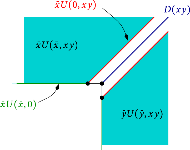
Figure 2: The series $D(xy)$
counts walks ending on the diagonal, and
$D(xy)$
counts walks ending on the diagonal, and $\bar x U(\bar x, xy)$
those ending above the diagonal.
$\bar x U(\bar x, xy)$
those ending above the diagonal.
We claim that the generating function of walks ending on the diagonal satisfies

The two terms involving D on the right-hand side count walks whose last step starts from the diagonal, and those involving U count walks whose last step starts from the lines $j=i\pm 1$
. For instance,
$j=i\pm 1$
. For instance, $\bar x U(0,xy)$
counts walks ending on the line
$\bar x U(0,xy)$
counts walks ending on the line $j=i+1$
, and the multiplication by
$j=i+1$
, and the multiplication by $ t \left (x \mathscr V_-(xy)\right )$
corresponds to adding a subdiagonal step. The factor
$ t \left (x \mathscr V_-(xy)\right )$
corresponds to adding a subdiagonal step. The factor $2$
accounts for the
$2$
accounts for the $x/y$
-symmetry of the model. The final term prevents from moving from
$x/y$
-symmetry of the model. The final term prevents from moving from $(-1,0)$
to
$(-1,0)$
to $(-1,-1)$
(or symmetrically). For walks ending (strictly) above the diagonal, we obtain
$(-1,-1)$
(or symmetrically). For walks ending (strictly) above the diagonal, we obtain

Again, the terms involving D (resp. U) count walks whose last step starts on (resp. above) the diagonal. The term involving $H_-(x)$
corresponds to walks that would enter the negative quadrant through the negative x-axis, and the term involving
$H_-(x)$
corresponds to walks that would enter the negative quadrant through the negative x-axis, and the term involving $\mathscr V_-(xy)$
counts walks that would in fact end on the diagonal. The final term corresponds to walks ending at
$\mathscr V_-(xy)$
counts walks that would in fact end on the diagonal. The final term corresponds to walks ending at $(-1,0)$
, extended by a South step: they have been subtracted twice, once in each of the previous two terms.
$(-1,0)$
, extended by a South step: they have been subtracted twice, once in each of the previous two terms.
We now perform the change of variables $(x,y) \mapsto (\bar x,xy)$
. This gives
$(x,y) \mapsto (\bar x,xy)$
. This gives


Using the first equation, we can eliminate $U(0,y)$
(and
$U(0,y)$
(and $U_{0,0}$
) from the second. Multiplying finally by
$U_{0,0}$
) from the second. Multiplying finally by $2y$
, we obtain the functional equation that we are going to focus on:
$2y$
, we obtain the functional equation that we are going to focus on:

with $\mathscr K(x,y) =1-tS(\bar x,xy)$
. It will be convenient to write it in terms of
$\mathscr K(x,y) =1-tS(\bar x,xy)$
. It will be convenient to write it in terms of $\mathscr S$
only: we thus observe that
$\mathscr S$
only: we thus observe that
 $$ \begin{align} (-1,-1) \in \mathcal S \Leftrightarrow (0,-1) \in \mathscr S \qquad \text{and} \qquad H_-(\bar x)=x \mathscr H_-(x), \end{align} $$
where we write
 $$ \begin{align} \quad \mathscr S(x,y)=\bar x \, \mathscr V_-(y) + \mathscr V_0(y) +x \mathscr V_+(y) = \bar y \mathscr H_-(x) +\mathscr H_0 +y \mathscr H_+(x). \end{align} $$
Lemma 2.1 For a step set $\mathcal S$
satisfying the assumptions (2.2), the series
$\mathcal S$
satisfying the assumptions (2.2), the series $U(x,y)$
and
$U(x,y)$
and $D(y)$
defined by (2.5) are related by
$D(y)$
defined by (2.5) are related by

with $\mathscr K(x,y):=K(\bar x,xy)=1-tS(\bar x,xy)$
. Note that
$\mathscr K(x,y):=K(\bar x,xy)=1-tS(\bar x,xy)$
. Note that $\mathscr K(x,y)$
is the kernel associated with the step set
$\mathscr K(x,y)$
is the kernel associated with the step set $\mathscr S$
defined by (2.7), which may not be
$\mathscr S$
defined by (2.7), which may not be $x/y$
-symmetric.
$x/y$
-symmetric.
This equation holds for the diagonal model $\mathcal S=\{ \nearrow , \nwarrow , \swarrow , \searrow \}$
as well, provided we define the series D and U by
$\mathcal S=\{ \nearrow , \nwarrow , \swarrow , \searrow \}$
as well, provided we define the series D and U by
 $$ \begin{align} C(x,y)=\bar x^2 U(\bar x^2, xy)+ D(xy)+ \bar y^2 U(\bar y^2,xy), \end{align} $$
and take $\mathscr S= \{\nearrow , \uparrow , \swarrow , \downarrow \}$
, that is,
$\mathscr S= \{\nearrow , \uparrow , \swarrow , \downarrow \}$
, that is,
 $$\begin{align*}\mathscr K(x,y)= 1-t \mathscr S(x,y)= 1-tS\left(\sqrt {\bar x},\sqrt xy\right)= 1-t(xy+y+\bar x\bar y +\bar y). \end{align*}$$
Proof We have already justified the equation under the assumptions (2.2). Now, consider the diagonal model. The only points $(i,j)$
that can be visited by a walk starting from
$(i,j)$
that can be visited by a walk starting from $(0,0)$
are such that
$(0,0)$
are such that $i+j$
is even. This allows us to write
$i+j$
is even. This allows us to write $C(x,y)$
as (2.13), where
$C(x,y)$
as (2.13), where $U(x,y)$
and
$U(x,y)$
and $D(y)$
are in
$D(y)$
are in $\mathbb {Q}[x,y][[t]]$
and
$\mathbb {Q}[x,y][[t]]$
and $\mathbb {Q}[y][[t]]$
, respectively. One then writes basic step-by-step equations for
$\mathbb {Q}[y][[t]]$
, respectively. One then writes basic step-by-step equations for $D(xy)$
and
$D(xy)$
and $\bar x^2 U(\bar x^2, xy)$
, and then performs the change of variables
$\bar x^2 U(\bar x^2, xy)$
, and then performs the change of variables $(x,y) \mapsto ( \sqrt {\bar x}, \sqrt x y)$
. This leads to the following counterparts of (2.8) and (2.9):
$(x,y) \mapsto ( \sqrt {\bar x}, \sqrt x y)$
. This leads to the following counterparts of (2.8) and (2.9):
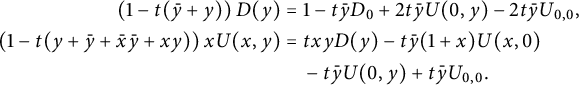 $$ \begin{align*} \left(1-t(\bar y+y)\right) D(y)&= 1-t\bar y D_0 +2t\bar y U(0,y)-2t\bar y U_{0,0},\\ \left(1-t(y+\bar y +\bar x\bar y+xy)\right)x U(x,y)& =txyD(y) -t\bar y (1+x) U(x,0)\\ &\quad -t\bar y U(0,y)+ t\bar y U_{0,0}. \end{align*} $$
The combination of these two equations gives
 $$ \begin{align} &2xy \left(1-t(y+\bar y+xy+\bar x\bar y)\right) U(x,y)=\nonumber\\ &\phantom{2xy (1-t(y+\bar y)}y+y\big(t(y+\bar y)+2txy-1\big) D(y) -2t(1+x)U(x,0)-tD_0, \end{align} $$
which coincides with (2.12).
Remark 2.2 The (single) equation in Lemma 2.1 really defines the two series $U(x,y)$
and
$U(x,y)$
and $D(y)$
. Indeed, equation (2.8) relating
$D(y)$
. Indeed, equation (2.8) relating $D(y)$
and
$D(y)$
and $U(0,y)$
can be recovered by setting
$U(0,y)$
can be recovered by setting $x=0$
in (2.12).
$x=0$
in (2.12).
Our solution of three-quadrant models will involve the generating function of walks with steps in $\mathscr S$
confined to the first (nonnegative) quadrant
$\mathscr S$
confined to the first (nonnegative) quadrant $\mathcal {Q}$
. This series
$\mathcal {Q}$
. This series $\mathscr Q(x,y)\equiv \mathscr Q(x,y;t)\in \mathbb {Q}[x,y][[t]]$
satisfies a similar looking equation [Reference Bousquet-Mélou and Mishna10]:
$\mathscr Q(x,y)\equiv \mathscr Q(x,y;t)\in \mathbb {Q}[x,y][[t]]$
satisfies a similar looking equation [Reference Bousquet-Mélou and Mishna10]:
where we have used the notation (2.11). This equation is simpler than (2.12), because its right-hand side, apart from the simple term $xy$
, is the sum of a function of x and a function of y. This is not the case in (2.12), because the factor
$xy$
, is the sum of a function of x and a function of y. This is not the case in (2.12), because the factor $\left (t \mathscr V_0(y)+ 2tx \mathscr V_+(y) -1\right )$
involves x. However, the square of this factor is a function of y only—modulo
$\left (t \mathscr V_0(y)+ 2tx \mathscr V_+(y) -1\right )$
involves x. However, the square of this factor is a function of y only—modulo $\mathscr K(x,y)$
. This property is already exploited in [Reference Raschel and Trotignon31].
$\mathscr K(x,y)$
. This property is already exploited in [Reference Raschel and Trotignon31].
Lemma 2.3 Let $\mathscr S$
be a collection of small steps, and define
$\mathscr S$
be a collection of small steps, and define $\mathscr V_+, \mathscr V_0$
, and
$\mathscr V_+, \mathscr V_0$
, and $\mathscr V_-$
by (2.11). Then
$\mathscr V_-$
by (2.11). Then
 $$\begin{align*}\big(t \mathscr V_0(y)+ 2tx \mathscr V_+(y) -1\big)^2=\Delta(y)-4tx \mathscr V_+(y) \mathscr K(x,y), \end{align*}$$
where $\mathscr K(x,y)=1-t\mathscr S(x,y)$
and
$\mathscr K(x,y)=1-t\mathscr S(x,y)$
and
 $$ \begin{align} \Delta(y)= \left(1-t\mathscr V_0(y)\right)^2-4t^2\mathscr V_-(y) \mathscr V_+(y) \end{align} $$
is the discriminant (in x) of $x\mathscr K(x,y)$
.
$x\mathscr K(x,y)$
.
The proof is a simple calculation, which we leave to the reader.
2.2 Invariants
We now define the notion of invariant that we use in this paper. We refer to [Reference Bernardi, Bousquet-Mélou and Raschel1, Reference Bernardi, Bousquet-Mélou and Raschel2] for a slightly different notion that applies to rational functions only. The definition that we adopt here allows us a uniform treatment of all the models that we solve, whereas in [Reference Bernardi, Bousquet-Mélou and Raschel2], quadrant walks with reverse Kreweras steps had to be handled by a different argument. We will only use our notion of invariants for small step models, but this subsection could actually be applied to any model in $ \{-1, 0, 1, 2, 3, \ldots \}^2$
.
$ \{-1, 0, 1, 2, 3, \ldots \}^2$
.
For reasons that are related to the form of the functional equation (2.12), we consider in this subsection a set of steps that we denote $\mathscr S$
rather than
$\mathscr S$
rather than $\mathcal S$
. Before all, observe that the series
$\mathcal S$
. Before all, observe that the series
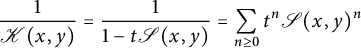 $$ \begin{align} \frac 1{\mathscr K(x,y)}=\frac 1{1-t \mathscr S(x,y)} =\sum_{n\ge 0} t^n \mathscr S(x,y)^n \end{align} $$
counts all walks with steps in $\mathscr S$
, starting from the origin, by the length (variable t) and the coordinates of the endpoint (variables x and y). The coefficient of
$\mathscr S$
, starting from the origin, by the length (variable t) and the coordinates of the endpoint (variables x and y). The coefficient of $t^n$
in this series is a Laurent polynomial in x and y. As soon as
$t^n$
in this series is a Laurent polynomial in x and y. As soon as $\mathscr S$
is not contained in a half-plane, the collection of these polynomials has unbounded degree and valuation.
$\mathscr S$
is not contained in a half-plane, the collection of these polynomials has unbounded degree and valuation.
Recall that $ \mathbb {Q}(x,y)((t))$
is the field of Laurent series in t with rational coefficients in x and y. We denote by
$ \mathbb {Q}(x,y)((t))$
is the field of Laurent series in t with rational coefficients in x and y. We denote by $ \mathbb {Q}_{\mathrm{mult}}(x,y)((t))$
the subring consisting of series in which for each n, the coefficient of
$ \mathbb {Q}_{\mathrm{mult}}(x,y)((t))$
the subring consisting of series in which for each n, the coefficient of $t^n$
is of the form
$t^n$
is of the form $p(x,y)/(d(x)d'(y))$
, where
$p(x,y)/(d(x)d'(y))$
, where $p(x,y) \in \mathbb {Q}[x,y]$
,
$p(x,y) \in \mathbb {Q}[x,y]$
, $d(x) \in \mathbb {Q}[x]$
, and
$d(x) \in \mathbb {Q}[x]$
, and $d'(y)\in \mathbb {Q}[y]$
. The reason why we focus on this subring is that:
$d'(y)\in \mathbb {Q}[y]$
. The reason why we focus on this subring is that:
-
• all the series that we handle are of this type;
-
• later (in the proof of Lemma 2.6) we will expand their coefficients as Laurent series in x and y, and with this condition the two expansions can be performed independently, without having to prescribe an order on x and y (as would be the case if we had to expand
$1/(x-y)$
, for instance).

Definition 2.1 A Laurent series $H(x,y)$
in
$H(x,y)$
in $ \mathbb {Q}_{\mathrm{mult}}(x,y)((t))$
is said to have poles of bounded order at
$ \mathbb {Q}_{\mathrm{mult}}(x,y)((t))$
is said to have poles of bounded order at $0$
if the collection of its coefficients (in the t-expansion) has poles of bounded order at
$0$
if the collection of its coefficients (in the t-expansion) has poles of bounded order at $x=0$
, and also at
$x=0$
, and also at $y=0$
. In other words, there exists a monomial
$y=0$
. In other words, there exists a monomial $x^i y^j$
such that
$x^i y^j$
such that $x^i y^j H(x,y)$
expands as a series in t whose coefficients have no pole at
$x^i y^j H(x,y)$
expands as a series in t whose coefficients have no pole at $x=0$
nor at
$x=0$
nor at $y=0$
.
$y=0$
.
Clearly, the series $ 1/{\mathscr K(x,y)}$
shown in (2.17) lies in
$ 1/{\mathscr K(x,y)}$
shown in (2.17) lies in $ \mathbb {Q}_{\mathrm{mult}}(x,y)((t))$
, but does not have poles of bounded order at
$ \mathbb {Q}_{\mathrm{mult}}(x,y)((t))$
, but does not have poles of bounded order at $0$
(unless
$0$
(unless $\mathscr S$
is contained in the first quadrant).
$\mathscr S$
is contained in the first quadrant).
Definition 2.2 (Divisibility)
Fix a step set $\mathscr S$
with kernel
$\mathscr S$
with kernel $\mathscr K(x,y)=1-t\mathscr S(x,y)$
. A Laurent series
$\mathscr K(x,y)=1-t\mathscr S(x,y)$
. A Laurent series $F(x,y)$
in
$F(x,y)$
in $ \mathbb {Q}_{\mathrm{mult}}(x,y)((t))$
is said to be divisible by
$ \mathbb {Q}_{\mathrm{mult}}(x,y)((t))$
is said to be divisible by $\mathscr K(x,y)$
if the ratio
$\mathscr K(x,y)$
if the ratio $F(x,y)/\mathscr K(x,y)$
has poles of bounded order at
$F(x,y)/\mathscr K(x,y)$
has poles of bounded order at $0$
.
$0$
.
Note that if $F(x,y)$
is in
$F(x,y)$
is in $ \mathbb {Q}_{\mathrm{mult}}(x,y)((t))$
, the ratio
$ \mathbb {Q}_{\mathrm{mult}}(x,y)((t))$
, the ratio $F(x,y)/\mathscr K(x,y)$
is always an element of
$F(x,y)/\mathscr K(x,y)$
is always an element of $ \mathbb {Q}_{\mathrm{mult}}(x,y)((t))$
(by (2.17)). The following alternative characterization of divisibility will not be used, but it may clarify the notion.
$ \mathbb {Q}_{\mathrm{mult}}(x,y)((t))$
(by (2.17)). The following alternative characterization of divisibility will not be used, but it may clarify the notion.
Lemma 2.4 Assume that $\mathscr K(x,y)$
has valuation
$\mathscr K(x,y)$
has valuation $-1$
and degree
$-1$
and degree $1$
in x and in y. The Laurent series
$1$
in x and in y. The Laurent series $F(x,y)$
in
$F(x,y)$
in $ \mathbb {Q}_{\mathrm{mult}}(x,y)((t))$
is divisible by
$ \mathbb {Q}_{\mathrm{mult}}(x,y)((t))$
is divisible by $\mathscr K(x,y)$
if and only if:
$\mathscr K(x,y)$
if and only if:
-
(1)
$F(x,y)$
has poles of bounded order at
$0$
; -
(2) if
$\mathscr X\equiv \mathscr X(y)$
(resp.
$\mathscr Y\equiv \mathscr Y(x)$
) denotes the unique root of
$\mathscr K(\cdot , y)$
(resp.
$\mathscr K(x, \cdot )$
) that is a formal power series in t (with coefficients in some algebraic closure of
$\mathbb {Q}(y)$
or
$\mathbb {Q}(x))$
, then
$F(\mathscr X,y)=F(x,\mathscr Y)=0$
.


Proof Assume that $F(x,y)$
is divisible by
$F(x,y)$
is divisible by $\mathscr K(x,y)$
, and write
$\mathscr K(x,y)$
, and write
 $$ \begin{align} F(x,y)= \mathscr K(x,y) H(x,y), \end{align} $$
where $H(x,y)$
has poles of bounded order at
$H(x,y)$
has poles of bounded order at $0$
. Since
$0$
. Since $\mathscr K(x,y)$
is a Laurent polynomial in x, y, and t, then
$\mathscr K(x,y)$
is a Laurent polynomial in x, y, and t, then $F(x,y)$
has poles of bounded order at
$F(x,y)$
has poles of bounded order at $0$
as well. Regarding Property (2), it suffices to prove it for
$0$
as well. Regarding Property (2), it suffices to prove it for $\mathscr X$
, by symmetry. Observe that the equation
$\mathscr X$
, by symmetry. Observe that the equation $\mathscr K(x, y)=0$
can be rewritten as
$\mathscr K(x, y)=0$
can be rewritten as
 $$\begin{align*}x= tx \mathscr S(x,y) = t \left( \mathscr V_-(y)+ x \mathscr V_0(y) + x^2 \mathscr V_+(y)\right). \end{align*}$$
This shows that exactly one of the roots of $\mathscr K(\cdot ,y)$
, denoted by
$\mathscr K(\cdot ,y)$
, denoted by $\mathscr X$
, is a formal power series in t; moreover, it has constant term
$\mathscr X$
, is a formal power series in t; moreover, it has constant term $0$
and coefficients in
$0$
and coefficients in $\mathbb {Q}(y)$
. Since
$\mathbb {Q}(y)$
. Since $F(x,y)$
and
$F(x,y)$
and $H(x,y)$
have poles of bounded order at
$H(x,y)$
have poles of bounded order at $0$
, the series
$0$
, the series $F(\mathscr X,y)$
and
$F(\mathscr X,y)$
and $H(\mathscr X,y)$
are well defined and belong to
$H(\mathscr X,y)$
are well defined and belong to $\mathbb {Q}(y)((t))$
. We now specialize x to
$\mathbb {Q}(y)((t))$
. We now specialize x to $\mathscr X$
in (2.18), and this proves that
$\mathscr X$
in (2.18), and this proves that $F(\mathscr X,y)=0$
.
$F(\mathscr X,y)=0$
.
Now, assume that the two conditions of the lemma hold, and let us prove that the series $H(x,y)$
defined by (2.18) has poles of bounded order at
$H(x,y)$
defined by (2.18) has poles of bounded order at $0$
. By symmetry, it suffices to prove this for the variable x. The second root of
$0$
. By symmetry, it suffices to prove this for the variable x. The second root of $\mathscr K(\cdot , y)$
is
$\mathscr K(\cdot , y)$
is
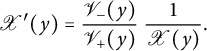 $$\begin{align*}\mathscr X'(y)= \frac{\mathscr V_-(y)}{\mathscr V_+(y)} \ \frac 1 {\mathscr X(y)}. \end{align*}$$
It is a Laurent series in t of valuation $-1$
, with coefficients in
$-1$
, with coefficients in $\mathbb {Q}(y)$
. A partial fraction expansion of
$\mathbb {Q}(y)$
. A partial fraction expansion of $1/\mathscr K(x,y)$
(in the variable x) gives
$1/\mathscr K(x,y)$
(in the variable x) gives
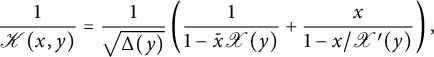 $$\begin{align*}\frac 1 {\mathscr K(x,y)}=\frac 1{\sqrt{\Delta(y)}} \left( \frac 1{1-\bar x \mathscr X(y)} + \frac x {1-x/\mathscr X'(y)}\right), \end{align*}$$
where $\Delta (y)$
is given by (2.16). By assumption,
$\Delta (y)$
is given by (2.16). By assumption, $F(x,y)$
has poles of bounded order at
$F(x,y)$
has poles of bounded order at $x=0$
. Since
$x=0$
. Since $\mathscr X(y)=\mathcal {O}(t)$
and
$\mathscr X(y)=\mathcal {O}(t)$
and $1/\mathscr X'(y)=\mathcal {O}(t)$
, only the first part of the above series has poles at
$1/\mathscr X'(y)=\mathcal {O}(t)$
, only the first part of the above series has poles at $x=0$
, and it suffices to prove that
$x=0$
, and it suffices to prove that
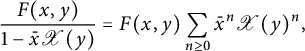 $$ \begin{align} \frac{F(x,y)}{1-\bar x\mathscr X(y)} = F(x,y) \sum_{n\ge 0} \bar x^n \mathscr X(y)^n, \end{align} $$
has poles of bounded order at $x=0$
. By assumption, there exists an integer i such that
$x=0$
. By assumption, there exists an integer i such that
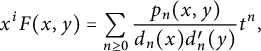 $$\begin{align*}x^i F(x,y)= \sum_{n\ge 0}\frac{p_n(x,y)}{ d_n(x) d^{\prime}_n(y)} t^n, \end{align*}$$
for polynomials $p_n$
,
$p_n$
, $d_n$
, and
$d_n$
, and $d^{\prime }_n$
such that
$d^{\prime }_n$
such that $d_n(0)\not =0$
. Then, by the assumption
$d_n(0)\not =0$
. Then, by the assumption $F(\mathscr X,y)=0$
, we have
$F(\mathscr X,y)=0$
, we have
 $$\begin{align*}\frac{ x^iF(x,y)}{1-\bar x\mathscr X} = \frac{x^iF(x,y)-\mathscr X^iF(\mathscr X,y)}{1-\bar x\mathscr X} = \!\sum_{n\ge 0}\!\left( \!\frac{p_n(x,y)}{ d_n(x) }- \frac{p_n(\mathscr X,y)}{d_n(\mathscr X) }\!\right) \!\frac x {x-\mathscr X} \frac{t^n}{d^{\prime}_n(y)}. \end{align*}$$
The nth summand can be written
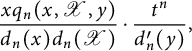 $$\begin{align*}\frac{ x q_n(x,\mathscr X,y)}{d_n(x) d_n(\mathscr X)}\cdot \frac{t^n}{d^{\prime}_n(y)}, \end{align*}$$
for some trivariate polynomial $q_n$
. As a series in t, it belongs to
$q_n$
. As a series in t, it belongs to $\mathbb {Q}_{\mathrm{mult}}(x,y)((t))$
, and its coefficients have no pole at
$\mathbb {Q}_{\mathrm{mult}}(x,y)((t))$
, and its coefficients have no pole at $x=0$
since
$x=0$
since $d(0)\not = 0$
(they are even multiples of x). We thus conclude that the series (2.19), as claimed, has poles of bounded order at
$d(0)\not = 0$
(they are even multiples of x). We thus conclude that the series (2.19), as claimed, has poles of bounded order at $x=0$
.
$x=0$
.
Definition 2.3 (Invariants)
Fix a step set $\mathscr S$
with kernel
$\mathscr S$
with kernel $\mathscr K(x,y)=1-t\mathscr S(x,y)$
. Let
$\mathscr K(x,y)=1-t\mathscr S(x,y)$
. Let $I(x)$
and
$I(x)$
and $J(y)$
be Laurent series in t with coefficients in
$J(y)$
be Laurent series in t with coefficients in $\mathbb {Q}(x)$
and
$\mathbb {Q}(x)$
and $\mathbb {Q}(y)$
, respectively. We say that
$\mathbb {Q}(y)$
, respectively. We say that $(I(x), J(y))$
is a pair of
$(I(x), J(y))$
is a pair of $\mathscr S$
-invariants if
$\mathscr S$
-invariants if $I(x)-J(y)$
is divisible by
$I(x)-J(y)$
is divisible by $\mathscr K(x,y)$
, in the sense of Definition 2.2.
$\mathscr K(x,y)$
, in the sense of Definition 2.2.
Note that $I(x)-J(y)$
is always an element of
$I(x)-J(y)$
is always an element of $\mathbb {Q}_{\mathrm{mult}}(x,y)((t))$
. Furthermore, if
$\mathbb {Q}_{\mathrm{mult}}(x,y)((t))$
. Furthermore, if $(I(x), J(y))$
is a pair of invariants, then
$(I(x), J(y))$
is a pair of invariants, then $I(x)$
and
$I(x)$
and $J(y)$
have poles of bounded order at
$J(y)$
have poles of bounded order at $0$
.
$0$
.
For any series $A\in \mathbb {Q}((t))$
, the pair
$A\in \mathbb {Q}((t))$
, the pair $(A,A)$
is a (trivial) invariant. More interesting examples will be given in the next subsection (see, for instance, (2.20)).
$(A,A)$
is a (trivial) invariant. More interesting examples will be given in the next subsection (see, for instance, (2.20)).
The term invariant comes from the fact that, if both roots $\mathscr X$
and
$\mathscr X$
and $\mathscr X'$
of
$\mathscr X'$
of $\mathscr K(\cdot , y)$
can be substituted for x in
$\mathscr K(\cdot , y)$
can be substituted for x in $I(x)$
, then
$I(x)$
, then $I(\mathscr X)=I(\mathscr X')$
. Of course, a similar observation holds for
$I(\mathscr X)=I(\mathscr X')$
. Of course, a similar observation holds for $J(y)$
.
$J(y)$
.
Lemma 2.5 The componentwise sum of two pairs of invariants $\left (I_1(x), J_1(y)\right )$
and
$\left (I_1(x), J_1(y)\right )$
and $\left (I_2(x), J_2(y)\right )$
is still a pair of invariants. The same holds for their componentwise product.
$\left (I_2(x), J_2(y)\right )$
is still a pair of invariants. The same holds for their componentwise product.
Proof The first result is obvious by linearity. For the second, we observe that
 $$ \begin{align*} I_1(x) I_2(x) -J_1(y) J_2(y)&= \left(I_1(x)-J_1(y)\right) I_2(x) +J_1(y) \left(I_2(x)-J_2(y)\right) \\ &= \mathscr K(x,y) \left( H_1(x,y)I_2(x) + J_1(y) H_2(x,y)\right), \end{align*} $$
where $H_k(x,y)=(I_k(x)-J_k(y))/\mathscr K(x,y)$
, for
$H_k(x,y)=(I_k(x)-J_k(y))/\mathscr K(x,y)$
, for $k=1,2$
. The result follows because series with poles of bounded order at
$k=1,2$
. The result follows because series with poles of bounded order at $0$
form a ring.
$0$
form a ring.
The following lemma is a key tool when playing with invariants.
Lemma 2.6 (Invariant lemma)
Let $I(x)$
and
$I(x)$
and $J(y)$
be Laurent series in t with coefficients in
$J(y)$
be Laurent series in t with coefficients in $\mathbb {Q}(x)$
and
$\mathbb {Q}(x)$
and $\mathbb {Q}(y)$
, respectively. Assume that for all n, the coefficient of
$\mathbb {Q}(y)$
, respectively. Assume that for all n, the coefficient of $t^n$
in the ratio series
$t^n$
in the ratio series
 $$\begin{align*}\frac{I(x)-J(y)}{\mathscr K(x,y)} \end{align*}$$
vanishes at $x=0$
and at
$x=0$
and at $y=0$
. Then
$y=0$
. Then $(I(x), J(y))$
is a pair of invariants by Definition 2.3, but in fact
$(I(x), J(y))$
is a pair of invariants by Definition 2.3, but in fact $I(x)$
and
$I(x)$
and $J(y)$
depend only on t, and are equal. That is, the above ratio is zero.
$J(y)$
depend only on t, and are equal. That is, the above ratio is zero.
Proof The argument is adapted from Lemma 4.13 in [Reference Bernardi, Bousquet-Mélou and Raschel2]. Let us assume, without loss of generality, that $I(x)$
and
$I(x)$
and $J(y)$
contain no negative power of t. By assumption, we have
$J(y)$
contain no negative power of t. By assumption, we have
 $$\begin{align*}I(x)-J(y) = xy \mathscr K(x,y) G(x,y),\\[-9pt] \end{align*}$$
where for each n, the coefficient of $t^n$
in
$t^n$
in $G(x,y) $
is of the form
$G(x,y) $
is of the form $p(x,y)/(d(x) d'(y))$
and has no pole at
$p(x,y)/(d(x) d'(y))$
and has no pole at $x=0$
nor
$x=0$
nor $y=0$
. Hence, this coefficient expands as a formal power series in x and y, and we consider
$y=0$
. Hence, this coefficient expands as a formal power series in x and y, and we consider $G(x,y)$
itself as an element of
$G(x,y)$
itself as an element of $\mathbb {Q}[[x,y,t]]$
. We define a total order on monomials
$\mathbb {Q}[[x,y,t]]$
. We define a total order on monomials $t^n x^i y^j$
, with
$t^n x^i y^j$
, with $(n,i,j) \in \mathbb {N}^3$
, by the lexicographic order on the exponents
$(n,i,j) \in \mathbb {N}^3$
, by the lexicographic order on the exponents $(n,i,j)$
. Observe that
$(n,i,j)$
. Observe that $xy\mathscr K(x,y) \in \mathbb {Q}[t,x,y]$
, and the smallest monomial that occurs in it is
$xy\mathscr K(x,y) \in \mathbb {Q}[t,x,y]$
, and the smallest monomial that occurs in it is $xy$
. Assume that
$xy$
. Assume that $G(x,y)\not =0$
, and let M be the smallest monomial in
$G(x,y)\not =0$
, and let M be the smallest monomial in $G(x,y)$
. Then
$G(x,y)$
. Then $xyM$
is the smallest monomial in
$xyM$
is the smallest monomial in $xy\mathscr K(x,y)G(x,y)$
, and hence in
$xy\mathscr K(x,y)G(x,y)$
, and hence in $I(x)-J(y)$
(once expanded as a series in t, whose coefficients are Laurent series in x or in y). However, the latter series cannot contain monomials involving both x and y. Hence,
$I(x)-J(y)$
(once expanded as a series in t, whose coefficients are Laurent series in x or in y). However, the latter series cannot contain monomials involving both x and y. Hence, $G(x,y)=0$
and the lemma is proved.
$G(x,y)=0$
and the lemma is proved.
2.3 Some known invariants
For each model $\mathscr S$
of Table 1, at least one nontrivial pair of invariants is already known from [Reference Bernardi, Bousquet-Mélou and Raschel2, Section 4], as we now review.
$\mathscr S$
of Table 1, at least one nontrivial pair of invariants is already known from [Reference Bernardi, Bousquet-Mélou and Raschel2, Section 4], as we now review.
Consider, for instance, the set $\mathscr S=\{\nearrow , \leftarrow , \downarrow \}$
of Kreweras’ steps, with
$\mathscr S=\{\nearrow , \leftarrow , \downarrow \}$
of Kreweras’ steps, with $\mathscr K(x,y)=1-t(xy+\bar x+\bar y)$
. The first pair of invariants exhibited in [Reference Bernardi, Bousquet-Mélou and Raschel2] is rational, and symmetric in x and y:
$\mathscr K(x,y)=1-t(xy+\bar x+\bar y)$
. The first pair of invariants exhibited in [Reference Bernardi, Bousquet-Mélou and Raschel2] is rational, and symmetric in x and y:
 $$\begin{align*}I_0(x)=\bar x^2-\bar x/t -x, \qquad J_0(y)=I_0(y).\\[-9pt] \end{align*}$$
Indeed, it is elementary to check that
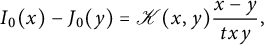 $$ \begin{align} I_0(x)-J_0(y)= \mathscr K(x,y) \frac{x-y}{txy},\\[-9pt]\nonumber \end{align} $$
and the “series” $\frac {x-y}{txy}$
has poles of bounded order at
$\frac {x-y}{txy}$
has poles of bounded order at $0$
. To describe the second pair, let
$0$
. To describe the second pair, let $\mathscr Q(x,y)$
be the generating function of quadrant walks with steps in
$\mathscr Q(x,y)$
be the generating function of quadrant walks with steps in $\mathscr S$
. Then
$\mathscr S$
. Then $\mathscr Q(x,y)$
satisfies the functional equation
$\mathscr Q(x,y)$
satisfies the functional equation
 $$ \begin{align} xy \mathscr K(x,y) \mathscr Q(x,y) =xy- tx \mathscr Q(x,0) -ty \mathscr Q(0,y),\\[-9pt]\nonumber \end{align} $$
and the $x/y$
-symmetry entails that
$x/y$
-symmetry entails that $\mathscr Q(x,0)=\mathscr Q(0,x)$
. Observe that
$\mathscr Q(x,0)=\mathscr Q(0,x)$
. Observe that
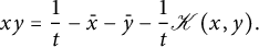 $$ \begin{align} xy = \frac 1 t - \bar x -\bar y- \frac 1 t \mathscr K(x,y).\\[-9pt]\nonumber \end{align} $$
Then the second pair of invariants $(I_1(x), J_1(y))$
is derived from (2.21) and (2.22):
$(I_1(x), J_1(y))$
is derived from (2.21) and (2.22):
 $$\begin{align*}I_1(x)= tx \mathscr Q(x,0)+ \bar x -\frac 1{2t}, \qquad J_1(y)= -I_1(y)= -ty\mathscr Q(0,y) -\bar y+\frac 1{2t}. \end{align*}$$
Indeed,
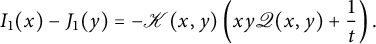 $$\begin{align*}I_1(x)-J_1(y) = -\mathscr K(x,y) \left(xy\mathscr Q(x,y)+\frac 1t\right). \end{align*}$$
More generally, it is proved in [Reference Bernardi, Bousquet-Mélou and Raschel2] that among the nine models $\mathscr S$
of Table 1, exactly the first five (those associated with a finite group) admit a pair of rational invariants
$\mathscr S$
of Table 1, exactly the first five (those associated with a finite group) admit a pair of rational invariants $(I_0(x), J_0(y))$
. We make them explicit in Table 3. On the other hand, the above construction of the
$(I_0(x), J_0(y))$
. We make them explicit in Table 3. On the other hand, the above construction of the $\mathscr Q$
-related pair
$\mathscr Q$
-related pair $(I_1(x), J_1(y))$
generalizes to all nine models, upon noticing that for each of them, the monomial
$(I_1(x), J_1(y))$
generalizes to all nine models, upon noticing that for each of them, the monomial $xy$
decouples explicitly as the sum of a function of x and a function of y—modulo
$xy$
decouples explicitly as the sum of a function of x and a function of y—modulo $\mathscr K$
:
$\mathscr K$
:
 $$ \begin{align} xy = f(x)+g(y)+ h(x,y)\mathscr K(x,y), \end{align} $$
for rational series $f(x), g(y)$
, and
$f(x), g(y)$
, and $h(x,y)$
having poles of bounded order at
$h(x,y)$
having poles of bounded order at $0$
. A possible choice of
$0$
. A possible choice of $f(x)$
and
$f(x)$
and $g(y)$
, borrowed from [Reference Bernardi, Bousquet-Mélou and Raschel2], is given in Tables 3 (for finite groups) and 4 (for infinite groups). The decoupling identity (2.23) allows us to rewrite the quadrant equation (2.15) as
$g(y)$
, borrowed from [Reference Bernardi, Bousquet-Mélou and Raschel2], is given in Tables 3 (for finite groups) and 4 (for infinite groups). The decoupling identity (2.23) allows us to rewrite the quadrant equation (2.15) as
 $$\begin{align*}\mathscr K(x,y) \left(h(x,y) -xy \mathscr Q(x,y)\right) = I_1(x)-J_1(y), \end{align*}$$
where

Since $h(x,y) -xy \mathscr Q(x,y)$
has poles of bounded order at
$h(x,y) -xy \mathscr Q(x,y)$
has poles of bounded order at $0$
, the pair
$0$
, the pair $(I_1(x), J_1(y))$
is indeed a pair of invariants. This pair is used in [Reference Bernardi, Bousquet-Mélou and Raschel2] to prove that
$(I_1(x), J_1(y))$
is indeed a pair of invariants. This pair is used in [Reference Bernardi, Bousquet-Mélou and Raschel2] to prove that $\mathscr Q(x,y;t)$
is algebraic (for finite group models) or D-algebraic (for infinite group models), for all models
$\mathscr Q(x,y;t)$
is algebraic (for finite group models) or D-algebraic (for infinite group models), for all models $\mathscr S$
in Table 1. The same approach applies to five other models
$\mathscr S$
in Table 1. The same approach applies to five other models $\mathscr S$
that are not relevant for this paper [Reference Bernardi, Bousquet-Mélou and Raschel2].
$\mathscr S$
that are not relevant for this paper [Reference Bernardi, Bousquet-Mélou and Raschel2].
Table 3: Rational $\mathscr S$
-invariants
$\mathscr S$
-invariants $(I_0,J_0)$
, and
$(I_0,J_0)$
, and $\mathscr S$
-decoupling of
$\mathscr S$
-decoupling of $xy$
by f and g for finite group models. The associated invariants
$xy$
by f and g for finite group models. The associated invariants $I_1(x), J_1(y)$
defined by (2.24) are algebraic.
$I_1(x), J_1(y)$
defined by (2.24) are algebraic.
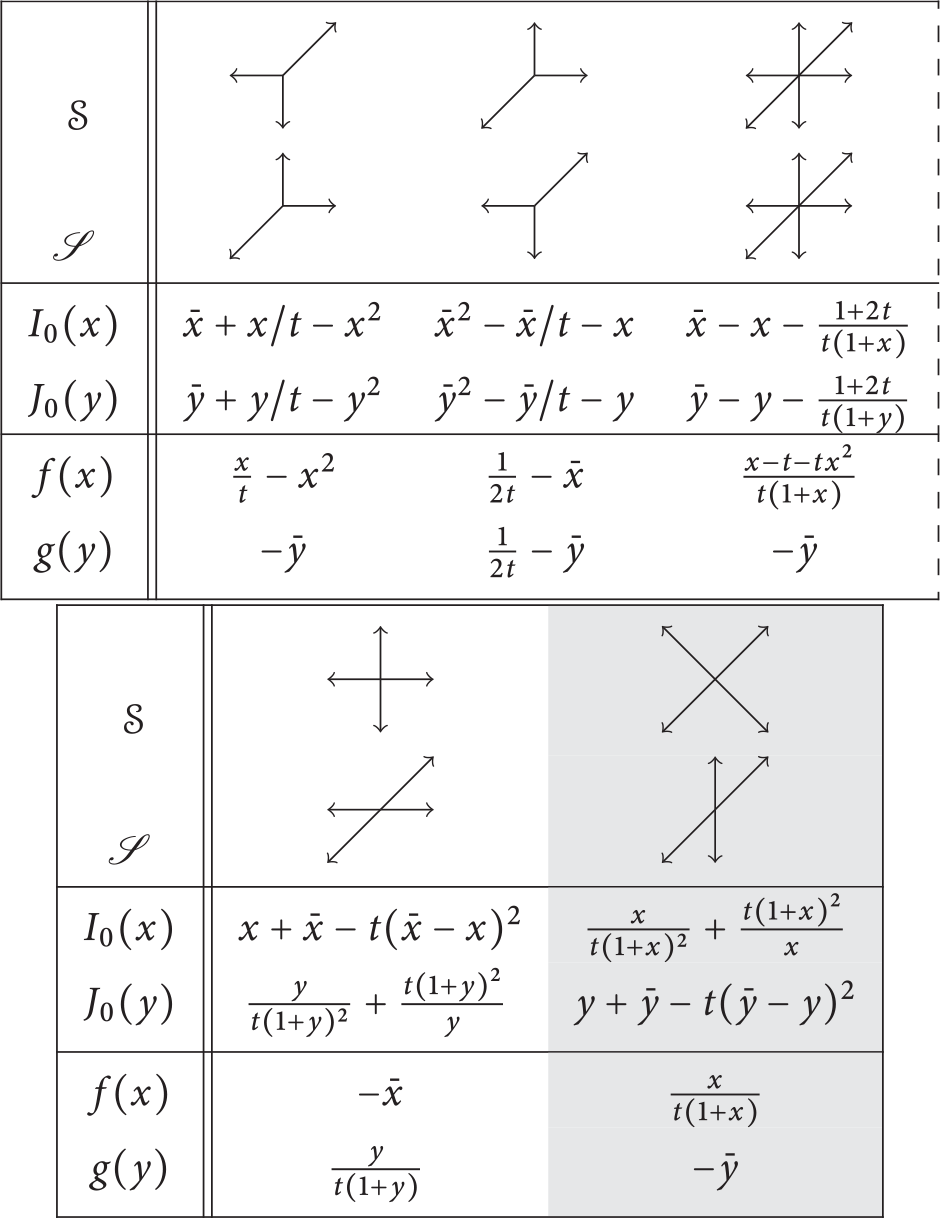
3 Decoupling and invariants for three-quadrant walks
3.1 A new type of decoupling
For the nine models $\mathscr S$
of Table 1, we have exhibited in the previous section invariants
$\mathscr S$
of Table 1, we have exhibited in the previous section invariants $(I_1(x),J_1(y))$
involving the generating function
$(I_1(x),J_1(y))$
involving the generating function $\mathscr Q(x,y;t)$
for quadrant walks, by combining the functional equation (2.15) with the decoupling of
$\mathscr Q(x,y;t)$
for quadrant walks, by combining the functional equation (2.15) with the decoupling of $xy$
modulo
$xy$
modulo $\mathscr K$
, given by (2.23).
$\mathscr K$
, given by (2.23).
Consider now the three-quadrant equation (2.12). One main difference with (2.15) is that the coefficient of $yD(y)$
, being
$yD(y)$
, being $\left (t \mathscr V_0(y)+ 2tx \mathscr V_+(y) -1\right )$
, involves both x and y. Our aim will be to write the right-hand side of (2.12) as the sum of a function of x and a function of y multiplied by
$\left (t \mathscr V_0(y)+ 2tx \mathscr V_+(y) -1\right )$
, involves both x and y. Our aim will be to write the right-hand side of (2.12) as the sum of a function of x and a function of y multiplied by $\left (t \mathscr V_0(y)+ 2tx \mathscr V_+(y) -1\right )$
, modulo the kernel
$\left (t \mathscr V_0(y)+ 2tx \mathscr V_+(y) -1\right )$
, modulo the kernel $\mathscr K(x,y)$
. Clearly, the only difficulty is to write the constant term y in this form. This turns out to be possible in exactly four of the nine cases, and this property is in fact related to “classical” decoupling of
$\mathscr K(x,y)$
. Clearly, the only difficulty is to write the constant term y in this form. This turns out to be possible in exactly four of the nine cases, and this property is in fact related to “classical” decoupling of $xy$
modulo the original model
$xy$
modulo the original model $\mathcal S$
(not
$\mathcal S$
(not $\mathscr S$
!).
$\mathscr S$
!).
Proposition 3.1 Let $\mathcal S$
be one of the nine models of Table 1, and
$\mathcal S$
be one of the nine models of Table 1, and $\mathscr S$
its companion model, with associated kernels
$\mathscr S$
its companion model, with associated kernels $K(x,y)$
and
$K(x,y)$
and $\mathscr K(x,y)$
, respectively. Define
$\mathscr K(x,y)$
, respectively. Define $\mathscr V_-$
,
$\mathscr V_-$
, $\mathscr V_0$
, and
$\mathscr V_0$
, and $\mathscr V_+$
by (2.11). The following conditions are equivalent:
$\mathscr V_+$
by (2.11). The following conditions are equivalent:
-
(a) There exist rational functions
$F(x)\in \mathbb {Q}(x,t)$
and
$G(y)\in \mathbb {Q}(y,t)$
such that the numerator of (3.1)contains a factor
$$ \begin{align} y- \left(t \mathscr V_0(y)+ 2tx \mathscr V_+(y) -1\right) G(y) - F(x) \end{align} $$
$xy\mathscr K(x,y)$
.
-
(b) There exist rational functions
$\mathsf {f(x)}\in \mathbb {Q}(x,t)$
and
$\mathsf {g}(y)\in \mathbb {Q}(y,t)$
such that the numerator of (3.2)contains a factor
$$ \begin{align} xy- \mathsf{f}(x) -\mathsf{g}(y) \end{align} $$
$xyK(x,y)$
.


The only models of Table 1 for which these properties hold are the three models of the Kreweras trilogy, and the $6$
th model. A solution is then given by
$6$
th model. A solution is then given by
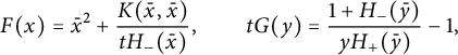 $$ \begin{align} F(x)= \bar x^2+ \frac{K(\bar x,\bar x)}{t H_-(\bar x)}, \qquad tG(y)= \frac{1+H_-(\bar y)}{y H_+(\bar y)} -1, \end{align} $$
and
 $$ \begin{align} \mathsf{f}(x)= \mathsf{g}(x)=\frac 1 2 \left( x^2+ \frac{K(x,x)}{t H_-(x)}\right). \end{align} $$
For this choice, stronger properties hold, as the rational functions (3.1) and (3.2) are then divisible by $\mathscr K(x,y)$
and
$\mathscr K(x,y)$
and $K(x,y)$
, respectively, in the sense of Definition 2.2.
$K(x,y)$
, respectively, in the sense of Definition 2.2.
The explicit values of the rational functions $F(x)$
and
$F(x)$
and $ G(y)$
are given in Table 5 for further reference.
$ G(y)$
are given in Table 5 for further reference.
Table 5: Decoupling of y in the form $y=c(x,y)G(y)+F(x)+\mathscr K(x,y) H(x,y)$
, with
$y=c(x,y)G(y)+F(x)+\mathscr K(x,y) H(x,y)$
, with $c(x,y)=t \mathscr V_0(y)+ 2tx \mathscr V_+(y) -1$
, for four symmetric models in the three-quadrant cone.
$c(x,y)=t \mathscr V_0(y)+ 2tx \mathscr V_+(y) -1$
, for four symmetric models in the three-quadrant cone.
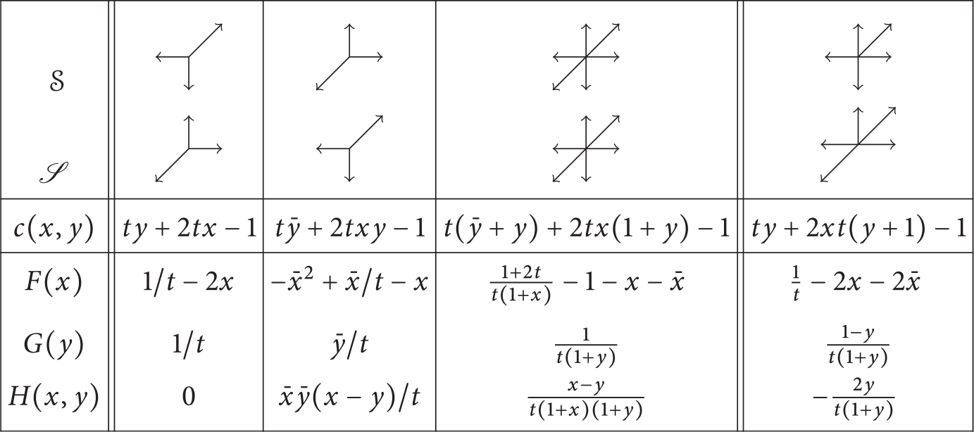
Remark 3.2 It follows from Lemma 2.4 that if a rational function is divisible by $K(x,y)$
, its numerator contains a factor
$K(x,y)$
, its numerator contains a factor $xyK(x,y)$
. However, the converse is wrong, as shown by
$xyK(x,y)$
. However, the converse is wrong, as shown by $xyK(x,y)/(x-t)$
. Hence, the term “stronger property” is used in the proposition.
$xyK(x,y)/(x-t)$
. Hence, the term “stronger property” is used in the proposition.
Proof of Proposition 3.1
We first consider the eight models with no step $\nwarrow $
nor
$\nwarrow $
nor $\searrow $
. Assume that the numerator of (3.1) contains a factor
$\searrow $
. Assume that the numerator of (3.1) contains a factor $xy\mathscr K(x,y)$
. Since
$xy\mathscr K(x,y)$
. Since $K(x,y)= \mathscr K(\bar x, xy)$
, it is equivalent to say that the numerator of
$K(x,y)= \mathscr K(\bar x, xy)$
, it is equivalent to say that the numerator of
 $$\begin{align*}xy-\left(t \mathscr V_0(xy)+2t\bar x \mathscr V_+(xy)-1\right) G(xy)-F(\bar x) \end{align*}$$
contains a factor $xyK(x,y)$
. Since
$xyK(x,y)$
. Since $K(x,y)=K(y,x)$
, the same holds for the numerator of
$K(x,y)=K(y,x)$
, the same holds for the numerator of
 $$\begin{align*}xy-\left(t \mathscr V_0(xy)+2t\bar y \mathscr V_+(xy)-1\right) G(xy)-F(\bar y), \end{align*}$$
and, by summing the two previous rational functions, for the numerator of
 $$\begin{align*}2xy-2 \left(t \mathscr V_0(xy)+t(\bar x+\bar y) \mathscr V_+(xy)-1\right) G(xy)-F(\bar x)-F(\bar y). \end{align*}$$
Since $S(x,y)=S(y,x)$
, it follows from the expression (2.6) of
$S(x,y)=S(y,x)$
, it follows from the expression (2.6) of $S(x,y)$
that
$S(x,y)$
that $\bar y \mathscr V_+(xy)=x \mathscr V_-(xy)$
. Hence, the coefficient of
$\bar y \mathscr V_+(xy)=x \mathscr V_-(xy)$
. Hence, the coefficient of $G(xy)$
in the above function is in fact
$G(xy)$
in the above function is in fact $2 K(x,y)$
. Since the denominator of
$2 K(x,y)$
. Since the denominator of $G(xy)$
cannot contain a factor
$G(xy)$
cannot contain a factor $xyK(x,y)$
(all steps of
$xyK(x,y)$
(all steps of $\mathcal S$
would be on the diagonal), we conclude that the numerator of
$\mathcal S$
would be on the diagonal), we conclude that the numerator of $2xy-F(\bar x)-F(\bar y)$
contains a factor
$2xy-F(\bar x)-F(\bar y)$
contains a factor $xyK(x,y)$
, which means that Condition (b) holds with
$xyK(x,y)$
, which means that Condition (b) holds with $\mathsf {f}(x)=\mathsf {g}(x)= F( \bar x)/2$
.
$\mathsf {f}(x)=\mathsf {g}(x)= F( \bar x)/2$
.
It is straightforward to adapt the above argument to the diagonal case, where now $S(x,y)=\mathscr S(\bar x^2,xy)= x^2\mathscr V_-(xy)+\mathscr V_0(xy)+\bar x^2 \mathscr V_+(xy)$
, with
$S(x,y)=\mathscr S(\bar x^2,xy)= x^2\mathscr V_-(xy)+\mathscr V_0(xy)+\bar x^2 \mathscr V_+(xy)$
, with $\bar y^2\mathscr V_+(xy)=x^2\mathscr V_-(xy)$
. One then finds a solution to Problem (b) with
$\bar y^2\mathscr V_+(xy)=x^2\mathscr V_-(xy)$
. One then finds a solution to Problem (b) with $\mathsf {f}(x)=\mathsf {g}(x)=F(\bar x^2)/2$
.
$\mathsf {f}(x)=\mathsf {g}(x)=F(\bar x^2)/2$
.
Conversely, assume that Condition (b) holds. As proved in [Reference Bernardi, Bousquet-Mélou and Raschel2, Section 4.2], then $\mathcal S$
is either one of three models of the Kreweras trilogy, or the
$\mathcal S$
is either one of three models of the Kreweras trilogy, or the $6$
th model of Table 1. Moreover, Condition (b) then holds for a pair
$6$
th model of Table 1. Moreover, Condition (b) then holds for a pair $(\mathsf {f}, \mathsf {g})$
such that
$(\mathsf {f}, \mathsf {g})$
such that $\mathsf {f}=\mathsf {g}$
: it suffices to take for
$\mathsf {f}=\mathsf {g}$
: it suffices to take for $ \mathsf {f}$
the half-sum of the two functions F and G of [Reference Bernardi, Bousquet-Mélou and Raschel2, Tables 4 and 5], and this yields (3.4). We leave it to the reader to check that the functions
$ \mathsf {f}$
the half-sum of the two functions F and G of [Reference Bernardi, Bousquet-Mélou and Raschel2, Tables 4 and 5], and this yields (3.4). We leave it to the reader to check that the functions $F(x)$
and
$F(x)$
and $G(y)$
defined by (3.3), and listed in Table 5, then satisfy Condition (a) of the lemma. Finally, since
$G(y)$
defined by (3.3), and listed in Table 5, then satisfy Condition (a) of the lemma. Finally, since $\mathsf {f}$
,
$\mathsf {f}$
, $\mathsf {g}$
, F, and G are Laurent polynomials in t, the same holds when dividing (3.1) by
$\mathsf {g}$
, F, and G are Laurent polynomials in t, the same holds when dividing (3.1) by $\mathscr K(x,y)$
or (3.2) by
$\mathscr K(x,y)$
or (3.2) by $K(x,y)$
, and the resulting ratios thus have poles of bounded order at zero. This establishes the claimed divisibility properties.
$K(x,y)$
, and the resulting ratios thus have poles of bounded order at zero. This establishes the claimed divisibility properties.
3.2 A new pair of invariants
We now restrict our attention to the four models of Table 5, for which the conditions of Proposition 3.1 hold. We return to the functional equation (2.12) that relates $U(x,y)$
and
$U(x,y)$
and $D(y)$
. We rewrite the first term y in the right-hand side using Proposition 3.1, and obtain
$D(y)$
. We rewrite the first term y in the right-hand side using Proposition 3.1, and obtain
 $$ \begin{align} \qquad \mathscr K(x,y) \left(2xy U(x,y)-H(x,y)\right) = \big(t \mathscr V_0(y)+ 2tx \mathscr V_+(y) -1\big) S(y)-R(x),\hspace{-20pt} \end{align} $$
with
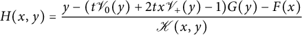 $$\begin{align*}H(x,y)= \frac{y-(t \mathscr V_0(y)+ 2tx \mathscr V_+(y) -1)G(y)-F(x)}{\mathscr K(x,y)} \end{align*}$$
and
The functions $F(x)$
,
$F(x)$
, $G(y)$
, and
$G(y)$
, and $H(x,y)$
are those of Table 5. Upon multiplying (3.5) by
$H(x,y)$
are those of Table 5. Upon multiplying (3.5) by
 $$\begin{align*}\left(t \mathscr V_0(y)+ 2tx \mathscr V_+(y) -1\right) S(y)+R(x), \end{align*}$$
and using Lemma 2.3, we exhibit a new pair of invariants.
Proposition 3.3 With the above notation, the pair $(I(x), J(y)):=(R(x)^2, \Delta (y) S(y)^2)$
is a pair of invariants for the step set
$(I(x), J(y)):=(R(x)^2, \Delta (y) S(y)^2)$
is a pair of invariants for the step set $\mathscr S$
, in the sense of Definition 2.3. More precisely,
$\mathscr S$
, in the sense of Definition 2.3. More precisely,
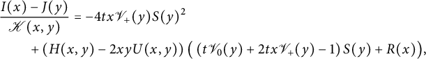 $$ \begin{align} &\frac{ I(x)-J(y)}{ \mathscr K(x,y) } = -4tx \mathscr V_+(y)S(y)^2 \nonumber\\ &\qquad+ \left( H(x,y) -2xy U(x,y) \right) \big( \left(t \mathscr V_0(y)+ 2tx \mathscr V_+(y) -1\right) S(y)+R(x)\big), \end{align} $$
where we recall that $\Delta (y)=\left (1-t\mathscr V_0(y)\right )^2-4t^2\mathscr V_-(y) \mathscr V_+(y)$
.
$\Delta (y)=\left (1-t\mathscr V_0(y)\right )^2-4t^2\mathscr V_-(y) \mathscr V_+(y)$
.
Proof The identity is straightforward, and we only need to check that all series that occur on the right-hand side of (3.7) have poles of bounded order at $0$
. First, this holds for the series F, G, and H (see Proposition 3.1 or Table 5). Then
$0$
. First, this holds for the series F, G, and H (see Proposition 3.1 or Table 5). Then $D(y)$
belongs to
$D(y)$
belongs to $\mathbb {Q}[y][[t]]$
,
$\mathbb {Q}[y][[t]]$
, $U(x,y)$
to
$U(x,y)$
to $\mathbb {Q}[x,y][[t]]$
, and
$\mathbb {Q}[x,y][[t]]$
, and $\mathscr H_-(x)$
is a Laurent polynomial in x. Thus, the series
$\mathscr H_-(x)$
is a Laurent polynomial in x. Thus, the series $R(x)$
and
$R(x)$
and $S(y)$
defined by (3.6) have poles of bounded order at
$S(y)$
defined by (3.6) have poles of bounded order at $0$
. Since
$0$
. Since $\mathscr V_0(y)$
and
$\mathscr V_0(y)$
and $\mathscr V_+(y)$
are Laurent polynomials in y, the conclusion follows.
$\mathscr V_+(y)$
are Laurent polynomials in y, the conclusion follows.
Remark 3.4 There is a useful alternative expression of $R(x)$
, and thus of
$R(x)$
, and thus of $I(x)=R(x)^2$
. Let us return to the basic functional equation (2.4) for
$I(x)=R(x)^2$
. Let us return to the basic functional equation (2.4) for $C(x,y)$
, written at
$C(x,y)$
, written at $(\bar x, \bar x)$
, and observe that
$(\bar x, \bar x)$
, and observe that $C_-(x)=xU(x,0)$
and
$C_-(x)=xU(x,0)$
and $C_{0,0}=D_0$
(see (2.5)). This gives
$C_{0,0}=D_0$
(see (2.5)). This gives
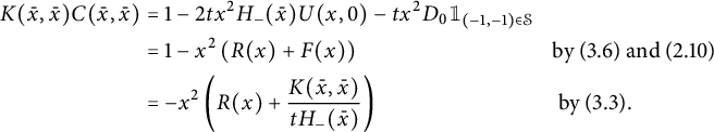
We conclude that
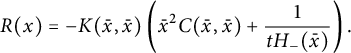 $$\begin{align*}R(x)=- K(\bar x, \bar x) \left(\bar x^2 C(\bar x, \bar x)+ \frac 1 {tH_-(\bar x)}\right). \end{align*}$$
In particular, for $x=1$
, we obtain
$x=1$
, we obtain
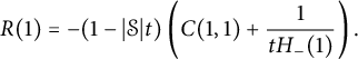 $$ \begin{align} R(1)= -(1-|\mathcal S|t) \left( C(1,1) + \frac 1 {tH_-(1)}\right). \end{align} $$
Since we are going to provide the value of $I(x)=R(x)^2$
explicitly, we will obtain an expression for the square of the above series. This is reflected in the characterization of
$I(x)=R(x)^2$
explicitly, we will obtain an expression for the square of the above series. This is reflected in the characterization of $C(1,1)$
already given for Kreweras’ model (see (1.15)). Further illustrations are (5.5), (6.9), and (7.7).
$C(1,1)$
already given for Kreweras’ model (see (1.15)). Further illustrations are (5.5), (6.9), and (7.7).
3.3 General strategy
Let us now describe the strategy that we are going to apply to each of the four models of Table 5, in Sections 4–7. For each of these models, we have at hand two, or sometimes three, pairs of $\mathscr S$
-invariants:
$\mathscr S$
-invariants:
-
• the pair
$(I(x),J(y))$
from Proposition 3.3; it involves the series
$U(x,0)=\bar x C_-(x)$
and
$D(y)$
, which are keys in the determination of the generating function
$C(x,y)$
of walks avoiding the negative quadrant; -
• a rational one,
$(I_0(x), J_0(y))$
, for the three models of the Kreweras trilogy (Table 3); -
• for all four models, the pair
$(I_1(x), J_1(y))$
defined by (2.24), where the functions f and g are given in Tables 3 and 4. This pair of invariants involves series counting quadrant walks with steps in
$\mathscr S$
, and these series are known. They are algebraic for the Kreweras trilogy [Reference Bousquet-Mélou and Mishna10], and D-algebraic for the last model [Reference Bernardi, Bousquet-Mélou and Raschel2].


Using Lemma 2.5, we are going to form polynomial combinations of these pairs to construct a new pair of invariants involving $U(x,0)$
and
$U(x,0)$
and $D(y)$
and satisfying the condition of Lemma 2.6—and thus trivial. This will give us expressions of
$D(y)$
and satisfying the condition of Lemma 2.6—and thus trivial. This will give us expressions of $I(x)$
and
$I(x)$
and $J(y)$
, and hence
$J(y)$
, and hence $U(x,0)$
and
$U(x,0)$
and $D(y)$
, in terms of some known quadrant series. For the Kreweras trilogy, an alternative would be to construct trivial invariants based on
$D(y)$
, in terms of some known quadrant series. For the Kreweras trilogy, an alternative would be to construct trivial invariants based on $(I(x), J(y))$
and
$(I(x), J(y))$
and $(I_0(x),J_0(y))$
only, as is done in [Reference Bernardi, Bousquet-Mélou and Raschel1, Reference Bernardi, Bousquet-Mélou and Raschel2] to (re)derive quadrant generating functions. However, exploiting the three pairs that we have at hand yields more direct derivations.
$(I_0(x),J_0(y))$
only, as is done in [Reference Bernardi, Bousquet-Mélou and Raschel1, Reference Bernardi, Bousquet-Mélou and Raschel2] to (re)derive quadrant generating functions. However, exploiting the three pairs that we have at hand yields more direct derivations.
4 Kreweras steps
In this section, we take $\mathcal S= \{\nearrow , \leftarrow , \downarrow \}$
, so that
$\mathcal S= \{\nearrow , \leftarrow , \downarrow \}$
, so that $\mathscr S=\{\rightarrow , \uparrow , \swarrow \}$
. We prove the results that were stated at the end of the introduction (Section 1.6): first the exact results in Section 4.1, then the asymptotic ones in Section 4.2. We refer to the Maple session available on the author’s web page (http://www.labri.fr/perso/bousquet/publis.html) for the details of the calculations.
$\mathscr S=\{\rightarrow , \uparrow , \swarrow \}$
. We prove the results that were stated at the end of the introduction (Section 1.6): first the exact results in Section 4.1, then the asymptotic ones in Section 4.2. We refer to the Maple session available on the author’s web page (http://www.labri.fr/perso/bousquet/publis.html) for the details of the calculations.
4.1 Generating functions
To begin with, we establish the expressions of $U(x,0)$
and
$U(x,0)$
and $D(y)$
.
$D(y)$
.
Proof of Theorems 1.1 and 1.2
The first equation in Theorem 1.1 is of course the basic functional equation (2.4). The $\mathscr S$
-invariants of Proposition 3.3 are
$\mathscr S$
-invariants of Proposition 3.3 are
 $$ \begin{align} I(x)=\left( 2tU(x,0)+2x-\frac 1 t \right)^2, \qquad J(y)=\Delta(y)\left(yD(y)+ \frac 1 t \right)^2 \end{align} $$
with $ \Delta (y)= (1-ty)^2-4t^2\bar y. $
The rational invariants
$ \Delta (y)= (1-ty)^2-4t^2\bar y. $
The rational invariants $(I_0,J_0)$
are given in Table 3 (but we will not use them, in fact). The invariants related to quadrant walks with steps in
$(I_0,J_0)$
are given in Table 3 (but we will not use them, in fact). The invariants related to quadrant walks with steps in $\mathscr S$
, defined by (2.24), are
$\mathscr S$
, defined by (2.24), are
 $$ \begin{align} I_1(x)=t\mathscr Q(x,0)-x/t+x^2, \qquad J_1(y) = -t\mathscr Q(0,y)-\bar y +t\mathscr Q_{0,0}. \end{align} $$
They satisfy
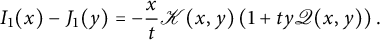 $$ \begin{align} I_1(x)-J_1(y)=-\frac x t \mathscr K(x,y) \left( 1+ty \mathscr Q(x,y)\right). \end{align} $$
We want to construct a pair $\left (\tilde I(x), \tilde J(y)\right )$
of invariants satisfying the condition of Lemma 2.6: the ratio
$\left (\tilde I(x), \tilde J(y)\right )$
of invariants satisfying the condition of Lemma 2.6: the ratio $(\tilde I(x)-\tilde J(y))/\mathscr K(x,y)$
should be a multiple of
$(\tilde I(x)-\tilde J(y))/\mathscr K(x,y)$
should be a multiple of $xy$
(here we are abusing terminology, since the property that we actually require involves the coefficient of
$xy$
(here we are abusing terminology, since the property that we actually require involves the coefficient of $t^n$
for each n). The ratio
$t^n$
for each n). The ratio $(I(x)-J(y))/\mathscr K(x,y)$
is the right-hand side of (3.7). It is easily seen to be a Laurent series in t with coefficients in
$(I(x)-J(y))/\mathscr K(x,y)$
is the right-hand side of (3.7). It is easily seen to be a Laurent series in t with coefficients in $\mathbb {Q}[x, y]$
, and in fact a multiple of x. It equals
$\mathbb {Q}[x, y]$
, and in fact a multiple of x. It equals $-4x/t$
at
$-4x/t$
at $y=0$
. Similarly, the ratio
$y=0$
. Similarly, the ratio $(I_1(x)-J_1(y))/\mathscr K(x,y)$
, derived from (4.3), is a multiple of x and equals
$(I_1(x)-J_1(y))/\mathscr K(x,y)$
, derived from (4.3), is a multiple of x and equals $-x/t$
at
$-x/t$
at $y=0$
. This leads us to introduce the following pair of invariants:
$y=0$
. This leads us to introduce the following pair of invariants:
 $$\begin{align*}\left(\tilde I(x), \tilde J(y)\right):= \big(I(x)-4I_1(x), J(y)-4J_1(y)\big), \end{align*}$$
which satisfies the condition of Lemma 2.6. This pair is thus of the form $(A,A)$
, where A is a series in t. Returning to the explicit values (4.1) and (4.2) of our invariants, this gives
$(A,A)$
, where A is a series in t. Returning to the explicit values (4.1) and (4.2) of our invariants, this gives
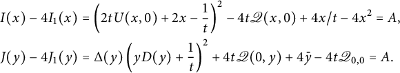 $$ \begin{align} \begin{aligned} I(x)-4I_1(x)&= \left( 2tU(x,0)+2x-\frac 1 t \right)^2-4t\mathscr Q(x,0)+4x/t-4x^2 =A, \\ J(y)-4J_1(y)&= \Delta(y)\left(yD(y)+ \frac 1 t \right)^2 +4 t\mathscr Q(0,y)+4\bar y -4t\mathscr Q_{0,0} =A. \end{aligned} \end{align} $$
To complete the solution, it suffices to:
-
• inject the known algebraic expressions of
$\mathscr Q(x,0)=\mathscr Q(0,x)$
and
$\mathscr Q_{0,0}$
, taken, for instance, from Proposition 14 in [Reference Bousquet-Mélou and Mishna10]. These expressions involve a series in t denoted by W in [Reference Bousquet-Mélou and Mishna10], which is the series V of Theorem 1.1. We refer to the Maple session for details; -
• specialize the second identity obtained in this way, of the form
(where
$$\begin{align*}\Delta(y)\left(yD(y)+ \frac 1 t \right)^2 -4J_1(y) =A, \end{align*}$$
$J_1(y)$
is now explicit), at
$y=V^2$
, which is the (only) root of
$\Delta (y)$
lying in
$\mathbb {Q}[[t]]$
. This gives
$$\begin{align*}A= -4 J_1(V^2)=2\,{\frac { (1-V^3)^{3/2}}{{V}^{2}}} +{\frac {{V}^{6}+12\,{V}^{3}+8}{4{V}^{2}}}. \end{align*}$$


These two ingredients yield, after elementary manipulations involving the equation $V=t(2+V^3)$
, the expressions announced in Theorems 1.1 and 1.2, which are those of
$V=t(2+V^3)$
, the expressions announced in Theorems 1.1 and 1.2, which are those of $I(x)/2$
and
$I(x)/2$
and $J(x)/2$
(recall that
$J(x)/2$
(recall that $U(x,0)=\bar x C_-(x)$
).
$U(x,0)=\bar x C_-(x)$
).
Since V has degree $3$
over
$3$
over $\mathbb {Q}(t)$
, it follows from these expressions that
$\mathbb {Q}(t)$
, it follows from these expressions that $C_-(x)$
and
$C_-(x)$
and $D(x)$
have degree at most
$D(x)$
have degree at most $24$
. This bound is proved to be tight by computing explicit minimal polynomials, at
$24$
. This bound is proved to be tight by computing explicit minimal polynomials, at $x=2$
for instance (this is lighter than keeping the indeterminate x). Now, the identities of Theorem 1.1 show that
$x=2$
for instance (this is lighter than keeping the indeterminate x). Now, the identities of Theorem 1.1 show that $C(x,y)$
will have degree
$C(x,y)$
will have degree $24\times 4=96$
at most, and at any rate the same degree as
$24\times 4=96$
at most, and at any rate the same degree as $xC_-(\bar x)+yC_-(\bar y)=U(\bar x,0)+U(\bar y,0)$
. So we only need to determine the degree of
$xC_-(\bar x)+yC_-(\bar y)=U(\bar x,0)+U(\bar y,0)$
. So we only need to determine the degree of $U(x,0)+U(y,0)$
, which we do at
$U(x,0)+U(y,0)$
, which we do at $x=2$
and
$x=2$
and $y=3$
(by successive eliminations as before). We find it to be
$y=3$
(by successive eliminations as before). We find it to be $96$
indeed, which concludes the proof of Theorems 1.1 and 1.2.
$96$
indeed, which concludes the proof of Theorems 1.1 and 1.2.
Now, we prove the results that deal with walks ending at a prescribed position $(i,j)$
.
$(i,j)$
.
Proof of Corollary 1.3
We begin with walks ending on the diagonal, the generating function of which is given in Theorem 1.2. We consider the series
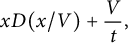 $$ \begin{align} x D(x/V) + \frac V t, \end{align} $$
which, due to the periodicity of the model and the fact that $V/t$
is a series in
$V/t$
is a series in $t^3$
, is also a series in
$t^3$
, is also a series in $t^3$
(or equivalently, in
$t^3$
(or equivalently, in $V^3$
) with coefficients in
$V^3$
) with coefficients in $\mathbb {Q}[x]$
. Using Theorem 1.2 and the identity
$\mathbb {Q}[x]$
. Using Theorem 1.2 and the identity $t=V/(2+V^3)$
, we can write
$t=V/(2+V^3)$
, we can write
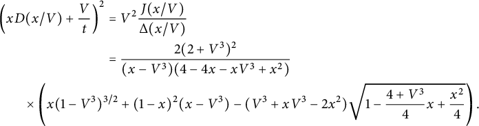 $$ \begin{align*} \left( x D(x/V) + \frac V t \right) ^2 &= V^2 \frac{J( x /V)}{\Delta( x /V)} \\ & =\frac {2(2+V^3)^2}{(x-V^3)(4-4x-xV^3+x^2)} \\&\hskip -20mm \times \left( x(1-V^3)^{3/2} +(1-x)^2 (x- V^3) - ( V^3+xV^3-2x^2) \sqrt{1- \frac{4+V^3} 4 x +\frac{x^2}4}\right). \end{align*} $$
The right-hand side appears as a formal power series in x, with constant term $(2+V^3)^2$
and coefficients in
$(2+V^3)^2$
and coefficients in $\mathbb {Q}[ \sqrt {1-V^3},1/V^3]$
. Upon taking square roots, we conclude that the series (4.5) is also a series in x with coefficients in
$\mathbb {Q}[ \sqrt {1-V^3},1/V^3]$
. Upon taking square roots, we conclude that the series (4.5) is also a series in x with coefficients in $\mathbb {Q}[\sqrt {1-V^3},1/V^3]$
. For
$\mathbb {Q}[\sqrt {1-V^3},1/V^3]$
. For $i\ge 0$
, the coefficient of
$i\ge 0$
, the coefficient of $x^{i+1}$
in this series is
$x^{i+1}$
in this series is $C_{i,i}/V^{i}$
. We have thus proved that
$C_{i,i}/V^{i}$
. We have thus proved that
 $$ \begin{align} \qquad D_i=C_{i,i}\in V^{i} \mathbb{Q}\left[ \sqrt{1-V^3},1/V^3\right], \quad \text{so that}\quad C_{i,i}\in t^i \mathbb{Q}\left[ \sqrt{1-V^3},1/V^3\right]. \hspace{-20pt}\end{align} $$
Since $V=t(2+V^3)$
, and
$V=t(2+V^3)$
, and $\sqrt {1-V^3}=1-2W$
by definition of W, the part of the corollary dealing with walks that end on the diagonal follows. We still retain the above more precise statement for further use. We obtain in particular the values of
$\sqrt {1-V^3}=1-2W$
by definition of W, the part of the corollary dealing with walks that end on the diagonal follows. We still retain the above more precise statement for further use. We obtain in particular the values of $C_{0,0}$
and
$C_{0,0}$
and $C_{1,1}$
given below Corollary 1.3. To obtain the claimed result for walks ending just above or below the diagonal (
$C_{1,1}$
given below Corollary 1.3. To obtain the claimed result for walks ending just above or below the diagonal ( $j-i=\pm 1$
, with
$j-i=\pm 1$
, with $i,j\ge 0$
), it suffices to note that
$i,j\ge 0$
), it suffices to note that
![]() due to the choice of steps. In particular, we thus obtain the value of
due to the choice of steps. In particular, we thus obtain the value of $C_{0,1}$
given below Corollary 1.3.
$C_{0,1}$
given below Corollary 1.3.
We go on with walks ending on the negative x-axis, the generating function of which is given in Theorem 1.1. By periodicity, the series
 $$ \begin{align} V \left(2t U(x/V)+2x/V-\frac 1 t\right) = V \left(2t \bar x V C_-(x/V)+2x/V-\frac 1 t\right) \end{align} $$
is a series in $t^3$
with coefficients in
$t^3$
with coefficients in $\mathbb {Q}[x]$
. Using Theorem 1.1, and the definition of W, we first rewrite its square in terms of x and W:
$\mathbb {Q}[x]$
. Using Theorem 1.1, and the definition of W, we first rewrite its square in terms of x and W:
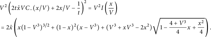 $$ \begin{align*} &V^2 \left(2t \bar x V C_-(x/V)+2x/V-\frac 1 t\right) ^2= V^2 I\left(\frac x V\right) \\ &=2\bar x \left( x(1-V^3)^{3/2} +(1-x)^2 (x- V^3) + ( V^3+xV^3-2x^2) \sqrt{1- \frac{4+V^3} 4 x +\frac{x^2}4}\right). \end{align*} $$
The right-hand side is a formal power series in x with constant term $2(1-V^3)^{3/2}+2+5V^3-V^6/4=4(1-W^2)(1+W)^2$
, whereas the coefficients of higher powers of x are polynomials in
$2(1-V^3)^{3/2}+2+5V^3-V^6/4=4(1-W^2)(1+W)^2$
, whereas the coefficients of higher powers of x are polynomials in $V^3$
. Given that
$V^3$
. Given that $V^3=4W(1-W)$
, we conclude that (4.7) has its coefficients in
$V^3=4W(1-W)$
, we conclude that (4.7) has its coefficients in $\sqrt {1-W^2}\, \mathbb {Q}[W, 1/(1-W^2)]$
. For
$\sqrt {1-W^2}\, \mathbb {Q}[W, 1/(1-W^2)]$
. For $i\ge 1$
, the coefficient of
$i\ge 1$
, the coefficient of $x^{i-1}$
in (4.7) is
$x^{i-1}$
in (4.7) is
Hence, using once again $V=t (2+V^3)$
, we find that
$V=t (2+V^3)$
, we find that
 $$ \begin{align} C_{-i,0} \in t^i \mathbb{Q}\left[\sqrt{1-W^2}, W, 1/V^3, 1/(1-W^2)\right]. \end{align} $$
We now introduce the series Z, which satisfies $\sqrt {1- W^2}= (1-Z^2)/(1+Z^2)$
. The corollary now follows for walks that end on the negative x-axis. We obtain in particular the expression (1.6) of
$\sqrt {1- W^2}= (1-Z^2)/(1+Z^2)$
. The corollary now follows for walks that end on the negative x-axis. We obtain in particular the expression (1.6) of $C_{-1,0}$
.
$C_{-1,0}$
.
Let us finally prove the corollary for any point $(i,j)$
in the three quadrant cone. Without loss of generality, we assume
$(i,j)$
in the three quadrant cone. Without loss of generality, we assume $j\ge i$
and argue by induction on
$j\ge i$
and argue by induction on $j\ge -1$
. If
$j\ge -1$
. If $j=-1$
, then
$j=-1$
, then $i<0$
and the result is obvious because
$i<0$
and the result is obvious because $C_{i,j}=0$
. The corollary has also been proved for
$C_{i,j}=0$
. The corollary has also been proved for $j=0$
,
$j=0$
, $j=i$
, and
$j=i$
, and $j=i+1$
. Now, assume that
$j=i+1$
. Now, assume that $j\ge 1$
and
$j\ge 1$
and $j\ge i+2$
. We clearly have
$j\ge i+2$
. We clearly have
 $$ \begin{align} C_{i,j-1} = t \left( C_{i-1, j-2} + C_{i+1,j-1} + C_{i,j} \right), \end{align} $$
and the result holds for the three series $C_{i,j-1}, C_{i-1, j-2} $
, and
$C_{i,j-1}, C_{i-1, j-2} $
, and $ C_{i+1,j-1} $
by the induction hypothesis. Thus, it holds for
$ C_{i+1,j-1} $
by the induction hypothesis. Thus, it holds for $C_{i,j}$
as well.
$C_{i,j}$
as well.
4.2 Asymptotics
We go on with the determination of the harmonic function.
Proof of Corollary 1.4
Let us first assume that we have established an estimate of the form (1.7) for $i=j\ge 0$
and for
$i=j\ge 0$
and for $i<0, j=0$
. For
$i<0, j=0$
. For $(i,j)\in \mathcal {C}$
, fix a walk w from
$(i,j)\in \mathcal {C}$
, fix a walk w from $(0,0)$
to
$(0,0)$
to $(i,j)$
in
$(i,j)$
in $\mathcal C$
, and let k be its length, with
$\mathcal C$
, and let k be its length, with $k+i+j\equiv 0$
mod
$k+i+j\equiv 0$
mod $3$
. Then
$3$
. Then $c_{i,j}(3m+k)\ge c_{0,0}(3m)$
(because one can concatenate w with a walk in
$c_{i,j}(3m+k)\ge c_{0,0}(3m)$
(because one can concatenate w with a walk in $\mathcal C$
starting and ending at
$\mathcal C$
starting and ending at $(0,0)$
, translated so that its starting point is
$(0,0)$
, translated so that its starting point is $(i,j)$
). Given the estimation of
$(i,j)$
). Given the estimation of $c_{0,0}(3m)$
, the numbers
$c_{0,0}(3m)$
, the numbers $c_{i,j}(n)$
cannot be
$c_{i,j}(n)$
cannot be $o(3^n n^{-7/4})$
.
$o(3^n n^{-7/4})$
.
Now, for $i\ge 0$
,
$i\ge 0$
,
 $$\begin{align*}c_{i,i}(n+1)=c_{i-1,i-1}(n)+ 2c_{i,i+1} (n). \end{align*}$$
This identity implies that an estimate of the form (1.7) also holds for $j=i+1 \ge 1$
, with
$j=i+1 \ge 1$
, with
 $$ \begin{align} 3H_{i,i}=H_{i-1,i-1}+2H_{i,i+1}. \end{align} $$
Here, we use the fact that $ 3H_{i,i}-H_{i-1,i-1}\not =0$
; otherwise,
$ 3H_{i,i}-H_{i-1,i-1}\not =0$
; otherwise, $c_{i,i+1} (n)$
would be
$c_{i,i+1} (n)$
would be $o(3^n n^{-7/4})$
, which we have excluded. Then the induction on j, with
$o(3^n n^{-7/4})$
, which we have excluded. Then the induction on j, with $j\ge i$
, that we have just used in the proof of the previous corollary, establishes (1.7) for all i and j, based on the following version of (4.9):
$j\ge i$
, that we have just used in the proof of the previous corollary, establishes (1.7) for all i and j, based on the following version of (4.9):
 $$\begin{align*}c_{i,j-1}(n+1) = c_{i-1, j-2}(n) + c_{i+1,j-1} (n)+ c_{i,j} (n). \end{align*}$$
The identity (1.8) saying that H is $\mathcal S^*$
-harmonic similarly follows from
$\mathcal S^*$
-harmonic similarly follows from
 $$\begin{align*}c_{i,j}(n+1) = c_{i-1, j-1}(n) + c_{i+1,j} (n)+ c_{i,j+1} (n). \end{align*}$$
Let us now define $\mathcal H(x,y)$
,
$\mathcal H(x,y)$
, $\mathcal H_-(x)$
, and
$\mathcal H_-(x)$
, and $\mathcal H_d(y)$
in terms of the numbers
$\mathcal H_d(y)$
in terms of the numbers $H_{i,j}$
as in Corollary 1.4. Then, using the harmonicity of H, we have
$H_{i,j}$
as in Corollary 1.4. Then, using the harmonicity of H, we have
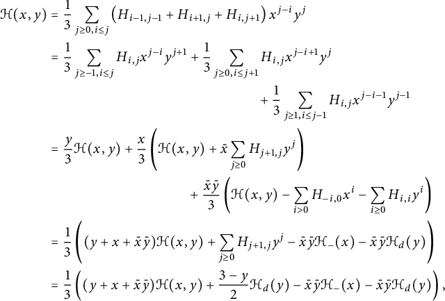 $$ \begin{align*} \mathcal H(x,y)& =\frac 1 3 \sum_{j\ge 0, i\le j } \left( H_{i-1,j-1}+ H_{i+1,j} + H_{i,j+1}\right)x^{j-i} y^{j} \\ &= \frac 1 3 \sum_{j\ge -1, i\le j } H_{i,j}x^{j-i} y^{j+1}+ \frac 1 3 \sum_{j\ge 0, i\le j+1 } H_{i,j}x^{j-i+1} y^{j} \\ &\hskip 51mm + \frac 1 3 \sum_{j\ge 1, i\le j-1 }H_{i,j}x^{j-i-1} y^{j-1} \\ &=\frac y 3 \mathcal H(x,y) +\frac x 3\left( \mathcal H(x,y) + \bar x\sum_{j \ge 0} H_{j+1,j} y^j\right) \\ &\hskip 34mm +\frac {\bar x \bar y}3\left( \mathcal H(x,y)- \sum_{i>0} H_{-i,0} x^{i}- \sum_{i\ge 0} H_{i,i} y^i\right) \\ &= \frac 1 3 \left( (y+x+\bar x\bar y)\mathcal H(x,y)+ \sum_{j \ge 0} H_{j+1,j} y^j- \bar x\bar y \mathcal H_-(x)-\bar x\bar y \mathcal H_d(y)\right) \\ &=\frac 1 3 \left( (y+x+\bar x\bar y)\mathcal H(x,y)+ \frac {3-y} 2 \mathcal H_d(y)- \bar x\bar y \mathcal H_-(x)-\bar x\bar y \mathcal H_d(y)\right), \end{align*} $$
where we have used (4.10) to express the final sum. This gives (1.10) upon regrouping terms.
At this stage, it remains to prove (1.7) for $i=j\ge 0$
and for
$i=j\ge 0$
and for $i<0, j=0$
, and to establish the announced values of the corresponding generating functions
$i<0, j=0$
, and to establish the announced values of the corresponding generating functions $\mathcal H_d(y)$
and
$\mathcal H_d(y)$
and $\mathcal H_-(x)$
. Let us begin with the numbers
$\mathcal H_-(x)$
. Let us begin with the numbers $c_{i,i}(n)$
, for n of the form
$c_{i,i}(n)$
, for n of the form $i+3m$
. Recall the form of
$i+3m$
. Recall the form of $C_{i,i}/t^i$
given by (4.6). An elementary singularity analysis of the series
$C_{i,i}/t^i$
given by (4.6). An elementary singularity analysis of the series $V^3$
(seen as a function of
$V^3$
(seen as a function of $t^3$
) shows that it has a unique dominant singularity, located at
$t^3$
) shows that it has a unique dominant singularity, located at $t^3=1/27$
. It increases on the interval
$t^3=1/27$
. It increases on the interval $[0,1/27]$
, and we have the following singular expansions:
$[0,1/27]$
, and we have the following singular expansions:
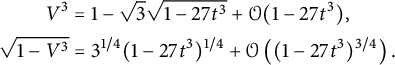 $$ \begin{align} V ^3&= 1-\sqrt 3 \sqrt{1-27t^3} + \mathcal{O}(1-27t^3), \\ \sqrt{1-V^3} &= 3^{1/4} (1-27t^3)^{1/4}+ \mathcal{O}\left((1-27t^3)^{3/4}\right). \nonumber \end{align} $$
Moreover, the equation $V=t(2+V^3)$
shows that V cannot vanish on its disk of convergence. In sight of (4.6),
$V=t(2+V^3)$
shows that V cannot vanish on its disk of convergence. In sight of (4.6), $C_{i,i}/t^i$
is thus an algebraic series in
$C_{i,i}/t^i$
is thus an algebraic series in $t^3$
, with radius of convergence at least
$t^3$
, with radius of convergence at least $1/27$
, taking a finite value at this point, and we expect a singular behavior in
$1/27$
, taking a finite value at this point, and we expect a singular behavior in $(1-27t^3)^{\alpha }$
for some
$(1-27t^3)^{\alpha }$
for some $\alpha \ge 1/4$
. Note that there cannot be any singularity other than
$\alpha \ge 1/4$
. Note that there cannot be any singularity other than $1/27$
on the circle of radius
$1/27$
on the circle of radius $1/27$
, because this is the only value of
$1/27$
, because this is the only value of $t^3$
for which V equals
$t^3$
for which V equals $1$
.
$1$
.
We now use Theorem 1.2 to express the series $(yD(y/t)+1)^2$
(which is a series in
$(yD(y/t)+1)^2$
(which is a series in $t^3$
) in terms of
$t^3$
) in terms of $V^3$
. Plugging in this expression, the above expansion of
$V^3$
. Plugging in this expression, the above expansion of $V^3$
then gives
$V^3$
then gives
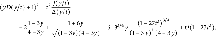 $$ \begin{align*} (yD(y/t)+1)^2 &= t^2 \frac{J(y/t)}{\Delta(y/t)}\\ & \hskip -12mm = 2\frac{1-3y}{4-3y} +\frac{1+6y}{\sqrt{(1-3y)(4-3y)}} - 6\cdot{3}^{3/4} y\,{\frac {{(1-27t^3)}^{3/4}}{ \left(1- 3\,y\right) ^{2} \left(4- 3\,y \right) }} + \mathcal{O}(1-27t^3). \end{align*} $$
We refer once again to the Maple session for details. It follows that as $t^3$
approaches
$t^3$
approaches $1/27$
,
$1/27$
,
 $$ \begin{align} D(y/t) = c_0(y) + c_1(y) (1-27t^3)^{3/4}+ \mathcal{O}(1-27t^3), \end{align} $$
where $c_0(y)$
is an algebraic function of y that we do not need to make explicit, and
$c_0(y)$
is an algebraic function of y that we do not need to make explicit, and
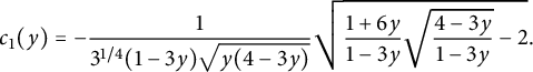 $$\begin{align*}c_1(y)= -\frac 1{3^{1/4}(1-3y)\sqrt{y(4-3y)}}\sqrt{\frac{1+6y}{1-3y} \sqrt{\frac{4-3y}{1-3y}}-2}. \end{align*}$$
By extracting from (4.12) the coefficient of $y^i$
, we obtain
$y^i$
, we obtain
 $$\begin{align*}C_{i,i} = t^i [y^i] c_0(y) + t^i [y^i] c_1(y) (1-27t^3)^{3/4}+ \mathcal{O}(1-27t^3), \end{align*}$$
so that, for $n=i+3m$
,
$n=i+3m$
,
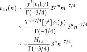 $$ \begin{align*} c_{i,i}(n) &\sim \frac{ [y^i] c_1(y) } {\Gamma(-3/4)}\, 27^m {m^{-7/4}}\\ &\sim \frac{ 3^{-i+7/4}[y^i] c_1(y) } {\Gamma(-3/4)}\, 3^n{n^{-7/4}}\\ & \sim -\frac{H_{i,i}}{\Gamma(-3/4)}\, 3^n{n^{-7/4}}, \end{align*} $$
where $ H_{i,i}=- 3^{7/4} [y^i] c_1(y/3). $
The announced expression of
$ H_{i,i}=- 3^{7/4} [y^i] c_1(y/3). $
The announced expression of $\mathcal H_d(y)=- 3^{7/4} c_1(y/3)$
follows.
$\mathcal H_d(y)=- 3^{7/4} c_1(y/3)$
follows.
Note that the above argument would fail if the coefficient of $y^i$
in
$y^i$
in $c_1(y)$
were zero. However, in this case,
$c_1(y)$
were zero. However, in this case, $c_{i,i}(n)$
would be
$c_{i,i}(n)$
would be $ o(3^n n^{-7/4})$
, which we have excluded at the beginning of the proof.
$ o(3^n n^{-7/4})$
, which we have excluded at the beginning of the proof.
We proceed similarly for walks ending on the negative x-axis. Equation (4.8) gives the form of $C_{-i,0}/t^i$
in terms of the series V and W. As
$C_{-i,0}/t^i$
in terms of the series V and W. As $V^3$
, the series W has a unique dominant singularity at
$V^3$
, the series W has a unique dominant singularity at $t^3=1/27$
. It increases on the interval
$t^3=1/27$
. It increases on the interval $[0, 1/27]$
and as
$[0, 1/27]$
and as $t^3$
approaches
$t^3$
approaches $1/27$
,
$1/27$
,
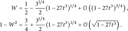 $$ \begin{align} \begin{aligned} W&= \frac 1 2 - \frac{3^{1/4}}2 (1-27t^3)^{1/4} + \mathcal{O}\left((1-27t^3)^{3/4}\right),\\ 1-W^2&=\frac 3 4 + \frac{3^{1/4}}2 (1-27t^3)^{1/4}+ \mathcal{O}\left(\sqrt{1-27t^3}\right). \end{aligned} \end{align} $$
Since W has nonnegative coefficients, and equals $1/2$
when
$1/2$
when $t^3=1/27$
, it remains away from the values
$t^3=1/27$
, it remains away from the values $\pm 1$
on the disk
$\pm 1$
on the disk $|t^3|<1/27$
. Hence, by (4.8), the series
$|t^3|<1/27$
. Hence, by (4.8), the series $C_{-i,0}/t^i$
has radius of convergence at least
$C_{-i,0}/t^i$
has radius of convergence at least $1/27$
, and no other singularity of modulus
$1/27$
, and no other singularity of modulus $1/27$
.
$1/27$
.
Then we consider the series $2C_-(x/t)+2x^2/t^3-x/t^3= x^2 I(x/t)/t^4$
, which is a series in
$2C_-(x/t)+2x^2/t^3-x/t^3= x^2 I(x/t)/t^4$
, which is a series in $t^3$
. We express its square in terms of
$t^3$
. We express its square in terms of $V^3$
using Theorem 1.1, and inject the singular expansion of
$V^3$
using Theorem 1.1, and inject the singular expansion of $V^3$
. This gives
$V^3$
. This gives
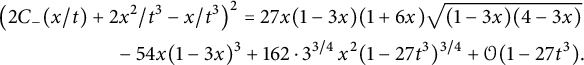 $$ \begin{align} &\left(2C_-(x/t)+2x^2/t^3-x/t^3\right)^2= 27x(1-3x)(1+6x)\sqrt{(1-3x)(4-3x)}\nonumber\\ &\phantom{(2C_-(x/t)+2}-54 x(1-3x)^3 + 162\cdot {3}^{3/4}\,{x}^{2}(1-27t^3)^{3/4} + \mathcal{O}(1-27t^3). \end{align} $$
We must be a bit careful with the sign when taking square roots. Indeed, both sides are $\mathcal {O}(x^2)$
, the coefficient of
$\mathcal {O}(x^2)$
, the coefficient of $x^2$
in the right-hand side is
$x^2$
in the right-hand side is
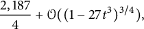 $$\begin{align*}{\frac{2,187}{4}}+ \mathcal{O}((1-27t^3)^{3/4}), \end{align*}$$
and this is the singular expansion of $(2C_{-1,0}/t-1/t^3)^2$
at
$(2C_{-1,0}/t-1/t^3)^2$
at $t^3=1/27$
. However, it follows from the expression (1.6) of
$t^3=1/27$
. However, it follows from the expression (1.6) of $C_{-1,0}$
, evaluated at
$C_{-1,0}$
, evaluated at $t=1/3$
(where
$t=1/3$
(where $Z=2-\sqrt 3$
), that at this point,
$Z=2-\sqrt 3$
), that at this point, $2C_{-1,0}/t-1/t^3= -27 \sqrt 3/2$
, with a minus sign. Hence, the square root of the right-hand side of (4.14) is
$2C_{-1,0}/t-1/t^3= -27 \sqrt 3/2$
, with a minus sign. Hence, the square root of the right-hand side of (4.14) is $-(2C_-(x/t)+2x^2/t^3-x/t^3)$
, and as
$-(2C_-(x/t)+2x^2/t^3-x/t^3)$
, and as $t^3$
approaches
$t^3$
approaches $1/27$
,
$1/27$
,
 $$\begin{align*}C_-(x/t) = \tilde c_0(x)+\tilde c_1(x) (1-27t^3)^{3/4} + \mathcal{O}(1-27t^3), \end{align*}$$
where
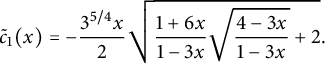 $$\begin{align*}\tilde c_1(x)=- \frac{3^{5/4} x}2 \sqrt{\frac{1+6x}{1-3x}\sqrt{\frac{4-3x}{1-3x}}+2} .\end{align*}$$
As we have just done for walks ending on the diagonal, we conclude that for n of the form $i+3m$
and
$i+3m$
and $i>0$
,
$i>0$
,
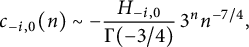 $$\begin{align*}c_{-i,0}(n) \sim -\frac{H_{-i,0}}{\Gamma(-3/4)}\, 3^n{n^{-7/4}}, \end{align*}$$
where $ H_{-i,0}=- 3^{7/4} [x^i] \tilde c_1(x/3). $
The announced expression of
$ H_{-i,0}=- 3^{7/4} [x^i] \tilde c_1(x/3). $
The announced expression of $\mathcal H_-(x)=- 3^{7/4} \tilde c_1(x/3)$
follows.
$\mathcal H_-(x)=- 3^{7/4} \tilde c_1(x/3)$
follows.
Remark 4.1
An invariant approach for harmonic functions. Let us now explain how we can predict the relation that we observed below Corollary 1.4 between the $\mathcal S^*$
-harmonic function
$\mathcal S^*$
-harmonic function $H_{i,j}$
in
$H_{i,j}$
in $\mathcal {C}$
and the
$\mathcal {C}$
and the $\mathscr S^*$
-harmonic function
$\mathscr S^*$
-harmonic function $h_{i,j}$
in
$h_{i,j}$
in $\mathcal {Q}$
.
$\mathcal {Q}$
.
As soon as an asymptotic estimate of the form (1.7) holds for the numbers $c_{i,j}(n)$
, the function
$c_{i,j}(n)$
, the function $H_{i,j}$
is
$H_{i,j}$
is $\mathcal S^*$
-harmonic in
$\mathcal S^*$
-harmonic in $\mathcal C$
, symmetric in the first diagonal, and the series
$\mathcal C$
, symmetric in the first diagonal, and the series $\mathcal H(x,y)$
defined by (1.9) satisfies (1.10). Denoting by
$\mathcal H(x,y)$
defined by (1.9) satisfies (1.10). Denoting by $c(x,y):=\frac 1 2 \left (2+xy^2-3xy\right ) $
the coefficient of
$c(x,y):=\frac 1 2 \left (2+xy^2-3xy\right ) $
the coefficient of $\mathcal H_d(y)$
in this equation, we observe that
$\mathcal H_d(y)$
in this equation, we observe that
 $$\begin{align*}c(x,y)^2= \frac {x^2\delta(y)} 4-3xy \mathscr K(x,y;1/3) = \frac {x^2\delta(y)} 4 + (1+xy^2+x^2y-3xy), \end{align*}$$
where $\delta (y)=y(y-4)(y-1)^2$
is the discriminant of
$\delta (y)=y(y-4)(y-1)^2$
is the discriminant of $3xy\mathscr K(x,y;1/3)$
with respect to x. This identity is of course closely related to Lemma 2.3. After multiplying (1.10) by
$3xy\mathscr K(x,y;1/3)$
with respect to x. This identity is of course closely related to Lemma 2.3. After multiplying (1.10) by
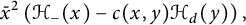 $$\begin{align*}\bar x^2\left( \mathcal H_-(x) - c(x,y)\mathcal H_d(y)\right), \end{align*}$$
we obtain
 $$ \begin{align} (1+xy^2+x^2y-3xy)\overline{\mathscr H}(x,y)= \bar x^2\,\mathcal H_-(x)^2- \frac {\delta(y)} 4\mathcal H_d(y)^2, \end{align} $$
where
 $$ \begin{align} \overline{\mathscr H}(x,y):= \bar x^2 \,\mathcal H ( x,y ) \left(\mathcal H_-(x) - c(x,y)\mathcal H_d(y) \right) +\bar x^2\, {\mathcal H_d}( y) ^{2}. \end{align} $$
Using the functional equation (1.10) satisfied by $\mathcal H(x,y)$
, we can check that
$\mathcal H(x,y)$
, we can check that $\overline {\mathscr H}(x,y)$
is a formal power series in x and y, and that, moreover,
$\overline {\mathscr H}(x,y)$
is a formal power series in x and y, and that, moreover,
 $$ \begin{align} \qquad \overline{\mathscr H}(x,0)= \bar x^2\,\mathcal H_-(x)^2 \qquad \text{and} \qquad \overline{\mathscr H}(0,y)= -\frac {\delta(y)} 4\, \mathcal H_d(y)^2+H_{-1,0}^2. \hspace{-20pt}\end{align} $$
In particular, if we denote $\overline {\mathscr H}(x,y)=\sum _{i,j\ge 0} \bar h_{i,j} x^i y^j$
, we have
$\overline {\mathscr H}(x,y)=\sum _{i,j\ge 0} \bar h_{i,j} x^i y^j$
, we have $\overline {\mathscr H}(0,0)=\bar h_{0,0}=H_{-1,0}^2$
. Equation (4.15) thus reads
$\overline {\mathscr H}(0,0)=\bar h_{0,0}=H_{-1,0}^2$
. Equation (4.15) thus reads
 $$\begin{align*}(1+xy^2+x^2y-3xy)\overline{\mathscr H}(x,y)=\overline{\mathscr H}(x,0)+\overline{\mathscr H}(0,y)-\overline{\mathscr H}(0,0), \end{align*}$$
which precisely means that the function $(\bar h_{i,j})_{(i,j)\in \mathcal {Q}}$
is
$(\bar h_{i,j})_{(i,j)\in \mathcal {Q}}$
is $\mathscr S^*$
-harmonic in the quadrant
$\mathscr S^*$
-harmonic in the quadrant $\mathcal {Q}$
.
$\mathcal {Q}$
.
Now, assume that there exists a unique positive $\mathscr S^*$
-harmonic function
$\mathscr S^*$
-harmonic function $h_{i,j}$
in
$h_{i,j}$
in $\mathcal {Q}$
(up to a multiplicative constant). The associated generating function is
$\mathcal {Q}$
(up to a multiplicative constant). The associated generating function is $\mathscr H(x,y)=\sum _{i,j\ge 0} h_{i,j} x^i y^j$
, where
$\mathscr H(x,y)=\sum _{i,j\ge 0} h_{i,j} x^i y^j$
, where $\mathscr H(x,0)=\mathscr H(0,x)$
is given by (1.14). Hence, if we assume that the above series
$\mathscr H(x,0)=\mathscr H(0,x)$
is given by (1.14). Hence, if we assume that the above series $\overline {\mathscr H}(x,y)$
has positive coefficients, then there exists a positive constant
$\overline {\mathscr H}(x,y)$
has positive coefficients, then there exists a positive constant $\kappa $
such that
$\kappa $
such that $\overline {\mathscr H}(x,y)=\kappa ^2 \mathscr H(x,y)$
. Returning to (4.17), we thus predict in particular that
$\overline {\mathscr H}(x,y)=\kappa ^2 \mathscr H(x,y)$
. Returning to (4.17), we thus predict in particular that
 $$\begin{align*}\mathcal H_-(x) =\kappa x \sqrt{\mathscr H(x,0)} \qquad \text{and} \qquad \mathcal H_d(y)=2\kappa\, \sqrt{-\frac { \mathscr H(0,y)-\mathscr H(0,0)}{ \delta(y)}}, \end{align*}$$
where the constant $\kappa $
must be
$\kappa $
must be
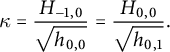 $$\begin{align*}\kappa = \frac{H_{-1,0}}{\sqrt{h_{0,0}}}= \frac{H_{0,0}}{\sqrt{h_{0,1}}}. \end{align*}$$
Using the expression (1.14) of $\mathscr H(x,0)=\mathscr H(0,x)$
, we can now check from the expressions (1.11) and (1.12) of
$\mathscr H(x,0)=\mathscr H(0,x)$
, we can now check from the expressions (1.11) and (1.12) of $\mathcal H_-(x)$
and
$\mathcal H_-(x)$
and $\mathcal H_d(y)$
that this prediction indeed holds true, with
$\mathcal H_d(y)$
that this prediction indeed holds true, with $\kappa =3$
.
$\kappa =3$
.
We finally complete this section with the enumeration of all walks avoiding the negative quadrant, regardless of their final position.
Proof of Corollary 1.6
We specialize the equations of Theorem 1.1 at $x= y=1$
. The first one gives the link between
$x= y=1$
. The first one gives the link between $C(1,1)$
and
$C(1,1)$
and $C_-(1)$
shown on the first line of (1.15) (this is in fact
$C_-(1)$
shown on the first line of (1.15) (this is in fact $I(1)/2$
), and the second one yields the expression on the second line. The degree of
$I(1)/2$
), and the second one yields the expression on the second line. The degree of $C(1,1)$
is found to be
$C(1,1)$
is found to be $24$
by elimination, first of the two square roots, and finally of V.
$24$
by elimination, first of the two square roots, and finally of V.
Now, for the asymptotics, we need more details about V than what we have used so far, which only involved $V^3$
(seen as a series in
$V^3$
(seen as a series in $t^3$
). The series V has three dominant singularities, located at
$t^3$
). The series V has three dominant singularities, located at $\zeta /3$
where
$\zeta /3$
where $\zeta $
is any cubic root of unity. The singular expansions of V at these points can be computed by combining
$\zeta $
is any cubic root of unity. The singular expansions of V at these points can be computed by combining $V=t(2+V^3)$
with the known expansion of
$V=t(2+V^3)$
with the known expansion of $V^3$
around
$V^3$
around $1/27$
(see (4.11)). Denoting
$1/27$
(see (4.11)). Denoting $\zeta _0=1$
and
$\zeta _0=1$
and $\zeta _\pm = (-1\pm i\sqrt 3)/2$
, we find that around any dominant singularity
$\zeta _\pm = (-1\pm i\sqrt 3)/2$
, we find that around any dominant singularity $\zeta /3$
,
$\zeta /3$
,
 $$ \begin{align} \qquad \frac V\zeta = 1- {(1-3t/\zeta)}^{1/2}+ (1-3 t/\zeta)/3-4/9 {(1-3t/\zeta)}^{3/2}+\mathcal{O} \left( {(1-3 t/\zeta)}^{2} \right). \hspace{-20pt}\end{align} $$
Observe that in the expression (1.15) of $(1-3t)^2 \left (C(1,1)+1/t\right )^2$
, the square root term involving
$(1-3t)^2 \left (C(1,1)+1/t\right )^2$
, the square root term involving
 $$\begin{align*}1-V\frac{4+V^3}4 +\frac{ V^2} 4 =\frac{(1-V)(2+V)(2-V+V^2)}4 \end{align*}$$
does not vanish for $|V|<1$
(but does vanish at
$|V|<1$
(but does vanish at $V=1$
of course). We now plug the above expansion of V in the expression of
$V=1$
of course). We now plug the above expansion of V in the expression of $(1-3t)^2 \left (C(1,1)+1/t\right )^2$
, extract square roots, and find the following behaviors, respectively, at
$(1-3t)^2 \left (C(1,1)+1/t\right )^2$
, extract square roots, and find the following behaviors, respectively, at $t=\zeta _0/3=1/3$
and
$t=\zeta _0/3=1/3$
and $t=\zeta _\pm /3$
:
$t=\zeta _\pm /3$
:
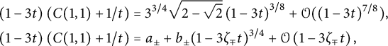 $$ \begin{align*} (1-3t) \left (C(1,1)+1/t\right) &= {3}^{3/4}\sqrt {2-\sqrt 2}\,{(1-3t)}^{3/8} +\mathcal{O}((1-3t)^{7/8}),\\ (1-3t) \left (C(1,1)+1/t\right) &= a_\pm + b_\pm (1-3\zeta_\mp t)^{3/4}+\mathcal{O} \left( 1-3\zeta_\mp t \right), \end{align*} $$
for some nonzero constants $a_\pm $
and
$a_\pm $
and $b_\pm $
. In sight of the factor
$b_\pm $
. In sight of the factor $(1-3t)$
on the left-hand side, we conclude that, as far as the first order of
$(1-3t)$
on the left-hand side, we conclude that, as far as the first order of $c_n$
is concerned, the only singularity that contributes is
$c_n$
is concerned, the only singularity that contributes is $1/3$
, and that
$1/3$
, and that $c_n$
satisfies (1.16).
$c_n$
satisfies (1.16).
5 Reverse Kreweras steps
In this section, we take $\mathcal S= \{\rightarrow , \uparrow , \swarrow \}$
, so that
$\mathcal S= \{\rightarrow , \uparrow , \swarrow \}$
, so that $\mathscr S=\{\nearrow , \leftarrow , \downarrow \}$
.
$\mathscr S=\{\nearrow , \leftarrow , \downarrow \}$
.
5.1 Statements of the results
We will establish the following counterpart of Theorems 1.1 and 1.2.
Theorem 5.1 The generating function $C(x,y)$
of walks with steps in
$C(x,y)$
of walks with steps in $\{\rightarrow , \uparrow , \swarrow \}$
starting from
$\{\rightarrow , \uparrow , \swarrow \}$
starting from $(0,0)$
and avoiding the negative quadrant is algebraic of degree
$(0,0)$
and avoiding the negative quadrant is algebraic of degree $96$
. It is given by the following equation:
$96$
. It is given by the following equation:
 $$\begin{align*}(1-t(x+y +\bar x\bar y)) C(x,y)=1 -t\bar x\bar y C_-(\bar x) -t\bar x\bar y C_-(\bar y)- t \bar x\bar y C_{0,0}, \end{align*}$$
where $C_{0,0}$
is algebraic of degree
$C_{0,0}$
is algebraic of degree $6$
and
$6$
and $C_-(x)$
is algebraic of degree
$C_-(x)$
is algebraic of degree $24$
. These series can be expressed explicitly in terms of the series V, W, and Z defined in Section 1 (see Table 2). Indeed,
$24$
. These series can be expressed explicitly in terms of the series V, W, and Z defined in Section 1 (see Table 2). Indeed,
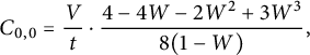 $$\begin{align*}C_{0,0}= \frac V t \cdot \frac{4-4W -2W^2+3W^3}{8 (1-W)}, \end{align*}$$
and
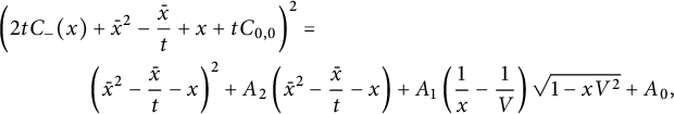 $$ \begin{align} &\left(2t C_-(x)+\bar x^2-\frac{\bar x}{ t} +x +t C_{0,0}\right)^2=\nonumber\\ &\phantom{2t C_-(x)+}\left(\bar x^2-\frac{\bar x}{t}-x\right)^2 +A_2\left(\bar x^2-\frac{\bar x}{t}-x\right)+ A_1\left( \frac 1 x - \frac 1 V\right) \sqrt{1-x V^2} + A_0, \end{align} $$
where the series $A_0$
,
$A_0$
, $A_1$
, and
$A_1$
, and $A_2$
belong to
$A_2$
belong to $\mathbb {Q}(t,Z)$
, with respective degrees
$\mathbb {Q}(t,Z)$
, with respective degrees $6,12$
, and
$6,12$
, and $6$
:
$6$
:
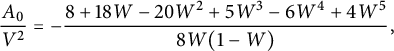 $$\begin{align*}\frac{ A_0}{V^2}= - \frac{8+18W-20W^2+5W^3-6W^4+4W^5}{8W (1-W)}, \end{align*}$$
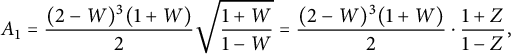 $$\begin{align*}A_1= \frac{(2-W)^3(1+W)}2 \sqrt{\frac{1+W}{1-W}} = \frac{(2-W)^3(1+W)}2 \cdot {\frac{1+Z}{1-Z}}, \end{align*}$$
and
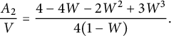 $$\begin{align*}\frac{A_2}V= \frac{4-4W -2W^2+3W^3}{4 (1-W)}. \end{align*}$$
The generating function $D(x)$
of walks ending on the diagonal is algebraic of degree
$D(x)$
of walks ending on the diagonal is algebraic of degree $24$
, given by
$24$
, given by
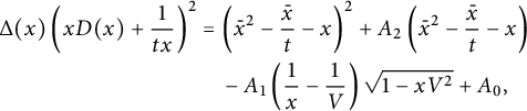 $$ \begin{align} \Delta(x) \left(xD(x)+ \frac{1}{tx}\right)^2&=\left(\bar x^2-\frac{\bar x}{t}-x\right)^2 +A_2\left(\bar x^2-\frac{\bar x}{t}-x\right)\nonumber\\&\quad - A_1\left( \frac 1 x - \frac 1 V\right) \sqrt{1-x V^2} + A_0, \end{align} $$
with the above values of $A_0, A_1, A_2$
, and
$A_0, A_1, A_2$
, and
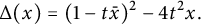 $$ \begin{align} \Delta(x)= (1-t\bar x)^2-4t^2x. \end{align} $$
For walks ending at a prescribed position, we obtain the following result.
Corollary 5.2 Let us define $V, W $
, and Z as above. For any
$V, W $
, and Z as above. For any $(i,j)\in \mathcal {C}$
, the generating function of walks avoiding the negative quadrant and ending at
$(i,j)\in \mathcal {C}$
, the generating function of walks avoiding the negative quadrant and ending at $(i,j)$
is algebraic of degree (at most)
$(i,j)$
is algebraic of degree (at most) $12$
and belongs to
$12$
and belongs to $\mathbb {Q}(t, Z)$
. More precisely,
$\mathbb {Q}(t, Z)$
. More precisely, $C_{i,j}/t^{i+j}$
belongs to
$C_{i,j}/t^{i+j}$
belongs to $\mathbb {Q}(Z)$
.
$\mathbb {Q}(Z)$
.
This holds obviously for the series $C_{0,0}$
given in Theorem 5.1. Note that this series coincides with the series
$C_{0,0}$
given in Theorem 5.1. Note that this series coincides with the series $C_{0,0}$
obtained for Kreweras walks (it suffices to rewrite
$C_{0,0}$
obtained for Kreweras walks (it suffices to rewrite $V/t$
in terms of W to obtain the form (1.5)): this is clear, upon reversing the direction of steps. Other examples are
$V/t$
in terms of W to obtain the form (1.5)): this is clear, upon reversing the direction of steps. Other examples are
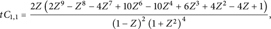 $$ \begin{align} tC_{1,1} = {\frac {2Z \left( 2 {Z}^{9}-{Z}^{8}-4 {Z}^{7}+10 {Z}^{6}-10 {Z}^{4}+6 {Z}^{3}+4 {Z}^{2}-4 Z+1 \right) } { \left(1- Z \right) ^{2} \left(1+ {Z}^{2} \right) ^{4}}}, \end{align} $$
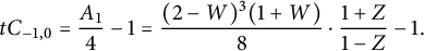 $$\begin{align*}t C_{-1,0} = \frac {A_1}4-1=\frac{(2-W)^3(1+W)}8 \cdot{\frac{1+Z}{1-Z}}-1. \end{align*}$$
The length generating function $C(1,1)$
of walks avoiding the negative quadrant can be characterized using the first two results of Theorem 5.1.
$C(1,1)$
of walks avoiding the negative quadrant can be characterized using the first two results of Theorem 5.1.
Corollary 5.3 The generating function $C(1,1)$
is algebraic of degree
$C(1,1)$
is algebraic of degree $24$
over
$24$
over $\mathbb {Q}(t)$
. It is given by
$\mathbb {Q}(t)$
. It is given by
 $$ \begin{align} (1-3t)^2(1+tC(1,1))^2=1- tA_2 + t^2A_1\left(1- \frac 1 V\right)\sqrt{1-V^2}+t^2A_0, \end{align} $$
where the series V, $A_0$
,
$A_0$
, $A_1$
, and
$A_1$
, and $A_2$
are those of Theorem 5.1. The asymptotic behavior of its nth coefficient
$A_2$
are those of Theorem 5.1. The asymptotic behavior of its nth coefficient $c_n$
can be obtained via singularity analysis:
$c_n$
can be obtained via singularity analysis:
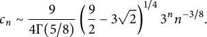 $$\begin{align*}c_n \sim \frac 9 {4\Gamma(5/8)} \left( \frac 9 2 - 3\sqrt 2\right) ^{1/4} 3^n n^{-3/8}. \end{align*}$$
Harmonic function
We have also derived the counterpart of Corollary 1.4, that is, an explicit harmonic function on $\mathcal {C}$
associated with the Kreweras step set
$\mathcal {C}$
associated with the Kreweras step set $\mathcal S^*=\{\leftarrow , \downarrow , \nearrow \}$
. We still have an asymptotic behavior of the form (1.7), this time with
$\mathcal S^*=\{\leftarrow , \downarrow , \nearrow \}$
. We still have an asymptotic behavior of the form (1.7), this time with $n\equiv i+j$
mod
$n\equiv i+j$
mod $3$
. We do not give here all details of the numbers
$3$
. We do not give here all details of the numbers $H_{i,j}$
, but simply the values of
$H_{i,j}$
, but simply the values of
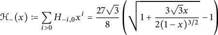 $$\begin{align*}\mathcal H_-(x):=\sum_{i>0} H_{-i,0} x^i=\frac {27\sqrt 3}{8} \left(\sqrt{1+ \frac{3\sqrt 3 x}{ 2(1-x)^{3/2}}}-1\right) \end{align*}$$
and
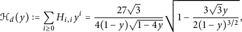 $$\begin{align*}\mathcal H_d(y):=\sum_{i\ge 0} H_{i,i}y^i =\frac{27\sqrt 3}{4(1-y) \sqrt{1-4y}} \sqrt{1- \frac{3\sqrt 3 y}{ 2(1-y)^{3/2}}}, \end{align*}$$
from which all numbers $H_{i,j}$
can be reconstructed via an equation that is the counterpart of (1.10). The proof is analogous to Kreweras’ case. Once again, details of the calculations can be found in our Maple session. For comparison, the number of quadrant
$H_{i,j}$
can be reconstructed via an equation that is the counterpart of (1.10). The proof is analogous to Kreweras’ case. Once again, details of the calculations can be found in our Maple session. For comparison, the number of quadrant $\mathscr S$
-walks of length n going from
$\mathscr S$
-walks of length n going from $(0,0)$
to
$(0,0)$
to $(i,j)$
is asymptotic to
$(i,j)$
is asymptotic to $h_{i,j} 3^n n^{-5/2}/\Gamma (-3/2)$
, with
$h_{i,j} 3^n n^{-5/2}/\Gamma (-3/2)$
, with
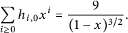 $$\begin{align*}\sum_{i\ge 0 } h_{i,0} x^i= \frac 9{(1-x)^{3/2}}. \end{align*}$$
5.2 Proofs for reverse Kreweras steps
Proof of Theorem 5.1
The first equation of the theorem is of course the basic functional equation (2.4). The functional equations (2.8) and (2.9) defining $D(y)$
and
$D(y)$
and $U(x,y)$
read
$U(x,y)$
read
 $$ \begin{align} (1-t\bar y) D(y) &=1 -t\bar y D_0+2tU(0,y) , \end{align} $$
 $$ \begin{align} x(1-t(\bar x+\bar y+xy)) U(x,y) &= tx y D(y)-tx\bar y U(x,0) -tU(0,y). \end{align} $$
The $\mathscr S$
-invariants of Proposition 3.3 are
$\mathscr S$
-invariants of Proposition 3.3 are
 $$ \begin{align} I(x)=\left( 2txU(x,0)+\frac 1 {x^2} -\frac 1 {tx} + x+ tD_0\right)^2, \qquad J(y)=\Delta(y)\left(yD(y)+ \frac 1 {ty} \right)^2, \end{align} $$
with $\Delta $
defined by (5.3). The rational invariants
$\Delta $
defined by (5.3). The rational invariants $(I_0,J_0)$
are given in Table 3:
$(I_0,J_0)$
are given in Table 3:
 $$ \begin{align} I_0(x)=\bar x^2-\bar x/t -x, \qquad J_0(y)=I_0(y). \end{align} $$
They satisfy
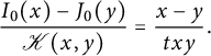 $$ \begin{align} \frac{I_0(x)-J_0(y)}{ \mathscr K(x,y)}= \frac{x-y}{txy}. \end{align} $$
The invariants related to quadrant walks with steps in $\mathscr S$
, defined by (2.24), are
$\mathscr S$
, defined by (2.24), are
 $$ \begin{align} \qquad I_1(x)= tx \mathscr Q(x,0)+ \bar x -\frac 1{2t}, \qquad J_1(y)= -ty\mathscr Q(0,y) -\bar y+\frac 1{2t} = -I_1(y).\hspace{-20pt} \end{align} $$
They satisfy
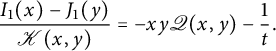 $$ \begin{align} \frac { I_1(x)-J_1(y)}{\mathscr K(x,y)}=- xy\mathscr Q(x,y)-\frac 1t. \end{align} $$
Applying the invariant lemma
As in the previous section, we want to combine the pair of invariants $(I(x),J(y))$
defined by (5.8) with those of (5.9) and (5.11) to form a pair
$(I(x),J(y))$
defined by (5.8) with those of (5.9) and (5.11) to form a pair $(\tilde I(x), \tilde J(y))$
satisfying the condition of Lemma 2.6. Since the conclusion of this lemma is that
$(\tilde I(x), \tilde J(y))$
satisfying the condition of Lemma 2.6. Since the conclusion of this lemma is that $\tilde I(x)$
and
$\tilde I(x)$
and $\tilde J(y)$
belong to
$\tilde J(y)$
belong to $\mathbb {Q}((t))$
, we must look for a polynomial combination of
$\mathbb {Q}((t))$
, we must look for a polynomial combination of $I(x)$
,
$I(x)$
, $I_0(x)$
, and
$I_0(x)$
, and $I_1(x)$
that, at least, has no pole at
$I_1(x)$
that, at least, has no pole at $x=0$
. In sight of the expansions of these three series at
$x=0$
. In sight of the expansions of these three series at $x=0$
, we are led to consider
$x=0$
, we are led to consider
 $$ \begin{align} \tilde I(x):= I(x) -I_0(x)^2 -A_2I_0(x)-A_1 I_1(x), \end{align} $$
with
 $$ \begin{align} A_2=2tD_0, \qquad A_1= 4(1+tU_{0,0}), \end{align} $$
which indeed has no pole at $x=0$
. Let us define accordingly
$x=0$
. Let us define accordingly
 $$ \begin{align} \tilde J(y):= J(y) -J_0(y)^2 -A_2J_0(y)-A_1 J_1(y), \end{align} $$
and examine whether $(\tilde I(x)-\tilde J(y))/\mathscr K(x,y)$
is a multiple of
$(\tilde I(x)-\tilde J(y))/\mathscr K(x,y)$
is a multiple of $xy$
. Denoting by
$xy$
. Denoting by $\operatorname {\mathrm {Rat}}$
,
$\operatorname {\mathrm {Rat}}$
, $\operatorname {\mathrm {Rat}}_0$
, and
$\operatorname {\mathrm {Rat}}_0$
, and $\operatorname {\mathrm {Rat}}_1$
the right-hand sides of (3.7), (5.10), and (5.12), respectively, we have
$\operatorname {\mathrm {Rat}}_1$
the right-hand sides of (3.7), (5.10), and (5.12), respectively, we have
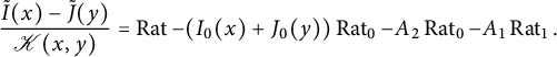 $$ \begin{align} \frac{\tilde I(x)-\tilde J(y)}{\mathscr K(x,y)}= \operatorname{\mathrm{Rat}} -(I_0(x)+J_0(y))\operatorname{\mathrm{Rat}}_0 -A_2 \operatorname{\mathrm{Rat}}_0-A_1 \operatorname{\mathrm{Rat}}_1. \end{align} $$
This ratio has poles of bounded order at $0$
. We first expand it around
$0$
. We first expand it around $x=0$
, and observe that it is
$x=0$
, and observe that it is $\mathcal {O}(1/x)$
. In order to prove that the coefficient of
$\mathcal {O}(1/x)$
. In order to prove that the coefficient of $1/x$
is in fact
$1/x$
is in fact $0$
, we use (5.6) (see our Maple session for details). In order to prove that the coefficient of
$0$
, we use (5.6) (see our Maple session for details). In order to prove that the coefficient of $x^0$
is also
$x^0$
is also $0$
, we use moreover the first term in the expansion of (5.7) at
$0$
, we use moreover the first term in the expansion of (5.7) at $x=0$
, which gives an expression of
$x=0$
, which gives an expression of $U^{\prime }_x(0,y)$
in terms of
$U^{\prime }_x(0,y)$
in terms of $U(0,y)$
,
$U(0,y)$
, $D(y)$
, and
$D(y)$
, and $U_{0,0}$
. Similarly, in order to prove that the ratio (5.16) is a multiple of y, we inject in its y-expansion (which is
$U_{0,0}$
. Similarly, in order to prove that the ratio (5.16) is a multiple of y, we inject in its y-expansion (which is $\mathcal {O}(y^0)$
) the expansion at
$\mathcal {O}(y^0)$
) the expansion at $y=0$
of (5.6), which relates
$y=0$
of (5.6), which relates $D_0$
,
$D_0$
, $D_1$
, and
$D_1$
, and $U_{0,0}$
, and the first term in the expansion of (5.7) at
$U_{0,0}$
, and the first term in the expansion of (5.7) at $y=0$
, which gives an expression of
$y=0$
, which gives an expression of $U^{\prime }_y(x,0)$
in terms of
$U^{\prime }_y(x,0)$
in terms of $U(x,0)$
and
$U(x,0)$
and $U_{0,0}$
. Then we happily conclude that the pair
$U_{0,0}$
. Then we happily conclude that the pair $(\tilde I(x), \tilde J(y))$
is independent of x and y, equal to
$(\tilde I(x), \tilde J(y))$
is independent of x and y, equal to $(A_0, A_0)$
for some series
$(A_0, A_0)$
for some series $A_0$
that depends on t only.
$A_0$
that depends on t only.
Recall the expression (5.11) of $I_1(x)$
in terms of the generating function
$I_1(x)$
in terms of the generating function $\mathscr Q(x,0)$
of quadrant walks with Kreweras steps. This series is known, and we obtain from Proposition 13 in [Reference Bousquet-Mélou and Mishna10]
$\mathscr Q(x,0)$
of quadrant walks with Kreweras steps. This series is known, and we obtain from Proposition 13 in [Reference Bousquet-Mélou and Mishna10]
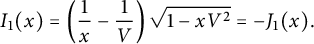 $$ \begin{align} I_1(x)= \left(\frac 1 x-\frac 1 V\right) \sqrt{1-x V^2}=-J_1(x). \end{align} $$
This gives the expressions (5.1) and (5.2) announced in Theorem 5.1, which are those of $I(x)$
and
$I(x)$
and $J(x)$
, but we still need to determine the three series
$J(x)$
, but we still need to determine the three series $A_0, A_1$
, and
$A_0, A_1$
, and $A_2$
.
$A_2$
.
The series
$A_0$
,
$A_1$
, and
$A_2$


In the Kreweras case (Section 4), we only had one unknown series to determine, denoted by A (see (4.4)). We derived it using the (only) root of $\Delta (y)$
that was finite at
$\Delta (y)$
that was finite at $t=0$
for this model. Now, with the new value of
$t=0$
for this model. Now, with the new value of $\Delta (y)$
, we have two such roots—but three series to determine. The third identity between the
$\Delta (y)$
, we have two such roots—but three series to determine. The third identity between the $A_i$
’s will follow from the fact that
$A_i$
’s will follow from the fact that $I(x)$
has a double root (see (5.8)).
$I(x)$
has a double root (see (5.8)).
We begin with a useful property, which tells us that $I_0(x)$
is (almost) the square of
$I_0(x)$
is (almost) the square of $I_1(x)$
. Indeed, the expressions of
$I_1(x)$
. Indeed, the expressions of $I_0(x)$
and
$I_0(x)$
and $I_1(x)$
, together with the definition (1.3) of V, imply that
$I_1(x)$
, together with the definition (1.3) of V, imply that
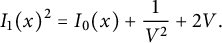 $$ \begin{align} I_1(x)^2= I_0(x)+ \frac 1 {V^2} + 2V. \end{align} $$
The series $J_1(y)=-I_1(y)$
and
$J_1(y)=-I_1(y)$
and $J_0(y)=I_0(x)$
are related by the same identity. (If we did not know the explicit expression (5.17) of
$J_0(y)=I_0(x)$
are related by the same identity. (If we did not know the explicit expression (5.17) of $I_1(x)$
, we could still derive this identity from the invariant lemma, which gives a polynomial relation between the pairs
$I_1(x)$
, we could still derive this identity from the invariant lemma, which gives a polynomial relation between the pairs $(I_1(x), J_1(y))$
and
$(I_1(x), J_1(y))$
and $(I_0(x), J_0(y))$
; this is how quadrant walks with steps in
$(I_0(x), J_0(y))$
; this is how quadrant walks with steps in $\mathscr S$
are solved in [Reference Bernardi, Bousquet-Mélou and Raschel2].)
$\mathscr S$
are solved in [Reference Bernardi, Bousquet-Mélou and Raschel2].)
Using this, and the definitions (5.13) and (5.15) of $\tilde I$
and
$\tilde I$
and $\tilde J$
, the fact that
$\tilde J$
, the fact that $\tilde I(x)= \tilde J(y) =A_0$
translates into
$\tilde I(x)= \tilde J(y) =A_0$
translates into
 $$ \begin{align} I(x)= P_4(I_1(x)), \qquad J(y)=P_4(J_1(y)), \end{align} $$
where
 $$\begin{align*}P_4(u)= \left(u^2- \frac 1 {V^2} - 2V\right)^2+A_2\left(u^2- \frac 1 {V^2} - 2V\right) + A_1 u+A_0. \end{align*}$$
Note that the identities of (5.19) are those that we would obtain from the invariant lemma by playing with the pairs $(I(x), J(y))$
and
$(I(x), J(y))$
and $(I_1(x),J_1(y))$
only, with no reference to
$(I_1(x),J_1(y))$
only, with no reference to $(I_0(x),J_0(y))$
.
$(I_0(x),J_0(y))$
.
As already mentioned, two roots of $\Delta (y)$
are finite at
$\Delta (y)$
are finite at $t=0$
. We denote them by
$t=0$
. We denote them by $Y_+$
and
$Y_+$
and $Y_-$
:
$Y_-$
:
 $$\begin{align*}Y_{\pm}= t \pm 2t^{5/2} +6t^4\pm 21 t^{11/2} +\mathcal O(t^7). \end{align*}$$
By replacing t by its expression in terms of V in $\Delta (y)$
, we see that
$\Delta (y)$
, we see that $Y_\pm $
are the roots of the following quadratic polynomial in Y:
$Y_\pm $
are the roots of the following quadratic polynomial in Y:
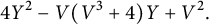 $$\begin{align*}4Y^2-V(V^3+4) Y+V^2. \end{align*}$$
The third root of $\Delta $
is
$\Delta $
is $1/V ^2$
. From this, and the expression (5.17) of
$1/V ^2$
. From this, and the expression (5.17) of $I_1(x)=-J_1(x)$
, we conclude that the values
$I_1(x)=-J_1(x)$
, we conclude that the values $J_1(Y_\pm )$
are roots of
$J_1(Y_\pm )$
are roots of
 $$\begin{align*}\tilde P_4(u)=4u^4V^4+V^2(V^6-20V^3-8)u^2-4V^9+12V^6-12V^3+4. \end{align*}$$
Since $J(y)$
contains a factor
$J(y)$
contains a factor $\Delta (y)$
and equals
$\Delta (y)$
and equals $P_4(J_1(y))$
, the values
$P_4(J_1(y))$
, the values $J_1(Y_\pm )$
are also roots of
$J_1(Y_\pm )$
are also roots of $P_4(u)$
, and hence of the following quadratic polynomial:
$P_4(u)$
, and hence of the following quadratic polynomial:
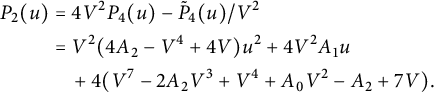 $$ \begin{align*} P_2(u)&= 4V^2P_4(u) -\tilde P_4(u)/V^2\\ &= V^2(4A_2-V^4+4V)u^2+4V^2A_1u\\&\quad +4(V^7-2A_2V^3+V^4+A_0V^2-A_2+7V). \end{align*} $$
Hence, $P_4(u)$
contains a factor
$P_4(u)$
contains a factor $P_2(u)$
.
$P_2(u)$
.
Now, consider the equation $I(X)=0$
, that is,
$I(X)=0$
, that is,
 $$\begin{align*}X=t \left(1+X^3+tX^2D_0+2tX^3U(X,0)\right). \end{align*}$$
From the form of this equation, we see that it admits a unique solution X in the ring $\mathbb {Q}[[t]]$
. The first terms in its expansion are
$\mathbb {Q}[[t]]$
. The first terms in its expansion are
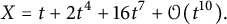 $$\begin{align*}X= t+ 2t^4+16 t^7 + \mathcal O(t^{10}). \end{align*}$$
Since $I(X)=0$
and
$I(X)=0$
and $I'(X)=0$
, it follows from (5.19) that
$I'(X)=0$
, it follows from (5.19) that $I_1(X)$
is a root of
$I_1(X)$
is a root of $P_4(u)$
, and even a double root, unless
$P_4(u)$
, and even a double root, unless $I^{\prime }_1(X)=0$
. However,
$I^{\prime }_1(X)=0$
. However, $I^{\prime }_1(X)= -1/t^2 + \mathcal {O}(t)$
, and hence
$I^{\prime }_1(X)= -1/t^2 + \mathcal {O}(t)$
, and hence $P_4(u)$
admits indeed
$P_4(u)$
admits indeed $I_1(X)$
as a double root. Moreover, we easily check that
$I_1(X)$
as a double root. Moreover, we easily check that $I_1(X)\not = J_1(Y_\pm )$
. Thus, we have found all roots of
$I_1(X)\not = J_1(Y_\pm )$
. Thus, we have found all roots of $P_4(u)$
, and we have the following factorization:
$P_4(u)$
, and we have the following factorization:
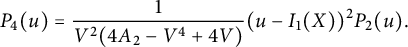 $$\begin{align*}P_4(u)= \frac 1 { V^2(4A_2-V^4+4V)} (u-I_1(X))^2 P_2(u). \end{align*}$$
(The multiplicative constant is adjusted using the leading coefficients of $P_2$
and
$P_2$
and $P_4$
.) By extracting the coefficients of
$P_4$
.) By extracting the coefficients of $u^3, \ldots , u^0$
in this identity, we obtain four polynomial equations that relate
$u^3, \ldots , u^0$
in this identity, we obtain four polynomial equations that relate $I_1(X)$
,
$I_1(X)$
, $A_0$
,
$A_0$
, $A_1$
, and
$A_1$
, and $A_2$
. By eliminating the first three series, we obtain a polynomial equation for
$A_2$
. By eliminating the first three series, we obtain a polynomial equation for $A_2$
. We determine which of its factors vanishes thanks to the first coefficients of
$A_2$
. We determine which of its factors vanishes thanks to the first coefficients of $A_2=2tD_0$
(see (5.14)), and, after introducing the series W, we obtain the value of
$A_2=2tD_0$
(see (5.14)), and, after introducing the series W, we obtain the value of $A_2$
given in Theorem 5.1. The values of
$A_2$
given in Theorem 5.1. The values of $A_1$
and
$A_1$
and $A_0$
follow similarly. We refer to our Maple session for details. Finally, the expression of
$A_0$
follow similarly. We refer to our Maple session for details. Finally, the expression of $C_{0,0}$
follows from
$C_{0,0}$
follows from $C_{0,0}=D_0=A_2/(2t)$
.
$C_{0,0}=D_0=A_2/(2t)$
.
Degrees
Let us now discuss the algebraic degrees of our generating functions. The expression of $C_{0,0}$
shows that it has degree at most
$C_{0,0}$
shows that it has degree at most $6$
, and this is easily checked to be tight by elimination of W and V. The expression of
$6$
, and this is easily checked to be tight by elimination of W and V. The expression of $I(x)$
shows that it belongs to an extension of degree
$I(x)$
shows that it belongs to an extension of degree $12$
of
$12$
of $\mathbb {Q}(t,x)$
: this can be seen by extending this field first by V (degree
$\mathbb {Q}(t,x)$
: this can be seen by extending this field first by V (degree $3$
), then W (degree
$3$
), then W (degree $2$
), and finally by
$2$
), and finally by $A_1\sqrt {1-xV^2}$
; the square of the latter series being in
$A_1\sqrt {1-xV^2}$
; the square of the latter series being in $\mathbb {Q}(x,t, V, W)$
(because
$\mathbb {Q}(x,t, V, W)$
(because $\frac {1+Z}{1-Z}= \sqrt {\frac {1+W}{1-W}} $
), this yields another extension of degree
$\frac {1+Z}{1-Z}= \sqrt {\frac {1+W}{1-W}} $
), this yields another extension of degree $2$
, resulting in total into a degree
$2$
, resulting in total into a degree $12$
at most for
$12$
at most for $I(x)$
. Since
$I(x)$
. Since $C_{0,0} \in \mathbb {Q}(W)$
, this implies that
$C_{0,0} \in \mathbb {Q}(W)$
, this implies that $U(x,0)$
has degree at most
$U(x,0)$
has degree at most $24$
. An effective elimination procedure shows that these bounds are tight. The same argument shows that
$24$
. An effective elimination procedure shows that these bounds are tight. The same argument shows that $J(x)$
has degree
$J(x)$
has degree $12$
, and
$12$
, and $D(x)$
degree
$D(x)$
degree $24$
. In fact,
$24$
. In fact, $I(x)$
and
$I(x)$
and $J(x)$
satisfy the same equation over
$J(x)$
satisfy the same equation over $\mathbb {Q}(t,x)$
, as shown by their respective expressions. Finally, the basic functional equation implies that the degree of
$\mathbb {Q}(t,x)$
, as shown by their respective expressions. Finally, the basic functional equation implies that the degree of $C(x,y)$
is the degree of
$C(x,y)$
is the degree of $C_-(x)+C_-(y)+C_{0,0}$
. We have seen that
$C_-(x)+C_-(y)+C_{0,0}$
. We have seen that $C_{0,0}$
belongs to
$C_{0,0}$
belongs to $\mathbb {Q}(t,V, W)$
, and that
$\mathbb {Q}(t,V, W)$
, and that $C_-(x)$
belongs to an extension of degree
$C_-(x)$
belongs to an extension of degree $4$
of
$4$
of $\mathbb {Q}(t,x, V, W)$
. Hence, the above sum belongs to an extension of
$\mathbb {Q}(t,x, V, W)$
. Hence, the above sum belongs to an extension of $\mathbb {Q}(t,x, V, W)$
of degree at most
$\mathbb {Q}(t,x, V, W)$
of degree at most $4\times 4=16$
, and thus has degree at most
$4\times 4=16$
, and thus has degree at most $16 \times 6=96$
. We compute its minimal polynomial over
$16 \times 6=96$
. We compute its minimal polynomial over $\mathbb {Q}(t)$
for
$\mathbb {Q}(t)$
for $x=2$
and
$x=2$
and $y=3$
, and find this bound to be tight.
$y=3$
, and find this bound to be tight.
Next, we establish the results that deal with walks ending at a prescribed point $(i,j)$
.
$(i,j)$
.
Proof of Corollary 5.2
We begin with walks ending on the diagonal, the generating function of which is given in Theorem 5.1. We consider the series
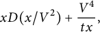 $$ \begin{align} x D(x/V^2) + \frac {V^4}{ tx}, \end{align} $$
which, due to the periodicity of the model and the properties of V, is a series in $t^3$
(or equivalently, in
$t^3$
(or equivalently, in $V^3$
) with coefficients in
$V^3$
) with coefficients in $\mathbb {Q}[\bar x,x]$
. Using the second part of Theorem 5.1, we first rewrite its square in terms of x and the series Z (this series is only needed because of the term
$\mathbb {Q}[\bar x,x]$
. Using the second part of Theorem 5.1, we first rewrite its square in terms of x and the series Z (this series is only needed because of the term $A_1$
, otherwise we could do with W as in Kreweras’ case). We thus obtain a (Laurent) series in x with rational coefficients in Z. The coefficient of
$A_1$
, otherwise we could do with W as in Kreweras’ case). We thus obtain a (Laurent) series in x with rational coefficients in Z. The coefficient of $x^{-2}$
in this series is
$x^{-2}$
in this series is ${V^8}/{t^2}$
. Hence, the square root of this series, which is (5.20), is also a series in x with coefficients in
${V^8}/{t^2}$
. Hence, the square root of this series, which is (5.20), is also a series in x with coefficients in $\mathbb {Q}(Z)$
. The coefficient of
$\mathbb {Q}(Z)$
. The coefficient of $x^i$
in (5.20) is
$x^i$
in (5.20) is $C_{i-1,i-1}/V^{2i-2}$
as soon as
$C_{i-1,i-1}/V^{2i-2}$
as soon as $i>0$
. The corollary thus follows for walks ending on the diagonal. In particular, for
$i>0$
. The corollary thus follows for walks ending on the diagonal. In particular, for $i=2$
, we obtain the expression (5.4) of
$i=2$
, we obtain the expression (5.4) of $C_{1,1}$
.
$C_{1,1}$
.
The same argument, starting now from
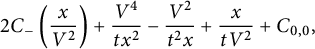 $$\begin{align*}2 C_-\left( \frac x {V^2}\right) + \frac{V^4}{tx^2} - \frac{V^2}{t^2x} + \frac x{tV ^2} + C_{0,0}, \end{align*}$$
establishes the result for walks ending on the negative x-axis, thanks to the expression of $I(x)$
. Indeed, one can show that this is a (Laurent) series in x with rational coefficients in Z, and the coefficient of
$I(x)$
. Indeed, one can show that this is a (Laurent) series in x with rational coefficients in Z, and the coefficient of $x^i$
in this series, for
$x^i$
in this series, for $i>0$
, is
$i>0$
, is
![]() . We obtain in particular the expression of
. We obtain in particular the expression of $C_{-1,0}=U_{0,0}$
given below Corollary 5.2 (but it also follows from (5.14) and the expression of
$C_{-1,0}=U_{0,0}$
given below Corollary 5.2 (but it also follows from (5.14) and the expression of $A_1$
).
$A_1$
).
We can now prove the corollary for any point $(i,j)$
in the three-quadrant cone. Without loss of generality, we assume that
$(i,j)$
in the three-quadrant cone. Without loss of generality, we assume that $j\ge i$
, and argue by induction on
$j\ge i$
, and argue by induction on $j\ge -1$
. The result is obvious when
$j\ge -1$
. The result is obvious when $j=-1$
(because then
$j=-1$
(because then $i<0$
and
$i<0$
and $C_{i,j}=0$
), and has just been established for
$C_{i,j}=0$
), and has just been established for $j=0$
. Since it has also been proved for
$j=0$
. Since it has also been proved for $j=i$
, we assume that
$j=i$
, we assume that $j\ge i+1$
and
$j\ge i+1$
and $j\ge 1$
. We have
$j\ge 1$
. We have
 $$\begin{align*}C_{i-1,j-1} = t \left( C_{i-1, j-2} + C_{i-2,j-1} + C_{i,j} \right), \end{align*}$$
and the result holds for the three series $ C_{i-1,j-1}, C_{i-1, j-2}, $
and
$ C_{i-1,j-1}, C_{i-1, j-2}, $
and $ C_{i-2,j-1} $
by the induction hypothesis. Thus, it holds for
$ C_{i-2,j-1} $
by the induction hypothesis. Thus, it holds for $C_{i,j}$
as well.
$C_{i,j}$
as well.
We conclude this section with the series $C(1,1)$
.
$C(1,1)$
.
Proof of Corollary 5.3
The value of $C(1,1)$
is obtained by specializing at
$C(1,1)$
is obtained by specializing at $x=y=1$
the first and third identities of Theorem 5.1. The fact that the degree of
$x=y=1$
the first and third identities of Theorem 5.1. The fact that the degree of $C(1,1)$
is
$C(1,1)$
is $24$
follows either by direct elimination, or by using the connection (3.8) between
$24$
follows either by direct elimination, or by using the connection (3.8) between $I(1)=R(1)^2$
and
$I(1)=R(1)^2$
and $C(1,1)$
and the polynomial equation (of degree
$C(1,1)$
and the polynomial equation (of degree $12$
) over
$12$
) over $\mathbb {Q}(t,x)$
that we have established for
$\mathbb {Q}(t,x)$
that we have established for $I(x)$
in the proof of Theorem 5.1.
$I(x)$
in the proof of Theorem 5.1.
The asymptotic result is obtained through singularity analysis, using the expressions of $A_0$
,
$A_0$
, $A_1$
, and
$A_1$
, and $A_2$
, and the singular properties of V and W (see (4.11), (4.13), (4.18), and the proof of Corollary 1.6 at the end of Section 4).
$A_2$
, and the singular properties of V and W (see (4.11), (4.13), (4.18), and the proof of Corollary 1.6 at the end of Section 4).
6 Double Kreweras steps
In this section, we take $\mathcal S= \{\rightarrow , \uparrow , \swarrow ,\nearrow , \leftarrow , \downarrow \}$
, so that
$\mathcal S= \{\rightarrow , \uparrow , \swarrow ,\nearrow , \leftarrow , \downarrow \}$
, so that $\mathscr S=\mathcal S$
.
$\mathscr S=\mathcal S$
.
6.1 Statements of the results
In order to state the counterparts of Theorems 1.1 and 1.2, we first need to introduce an extension of $\mathbb {Q}(t)$
of degree
$\mathbb {Q}(t)$
of degree $16$
, illustrated in Figure 3.
$16$
, illustrated in Figure 3.
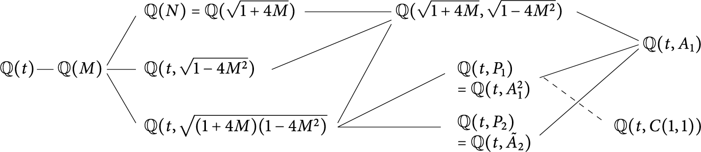
Figure 3: The extension of $\mathbb {Q}(t)$
of degree
$\mathbb {Q}(t)$
of degree $16$
generated by
$16$
generated by $A_1$
. All elementary extensions have degree
$A_1$
. All elementary extensions have degree $2$
. The series
$2$
. The series $C(1,1)$
has degree
$C(1,1)$
has degree $16$
over
$16$
over $\mathbb {Q}(t)$
, as
$\mathbb {Q}(t)$
, as $A_1$
, but lies in a different extension of
$A_1$
, but lies in a different extension of $\mathbb {Q}(t)$
.
$\mathbb {Q}(t)$
.
First, we define $M\equiv M(t)$
as the unique formal power series in t satisfying
$M\equiv M(t)$
as the unique formal power series in t satisfying
 $$\begin{align*}M=t(1+2M+4M^2). \end{align*}$$
The coefficient of $t^{n+1}$
in M is
$t^{n+1}$
in M is $2^n$
times the nth Motzkin number, hence the notation M. The series
$2^n$
times the nth Motzkin number, hence the notation M. The series $M/t$
is known to count walks with steps in
$M/t$
is known to count walks with steps in $\mathcal S$
confined to the North-West quadrant
$\mathcal S$
confined to the North-West quadrant $\{(i,j): i\le 0, j \ge 0\}$
(see [Reference Bousquet-Mélou and Mishna10, Proposition 10]). Note that
$\{(i,j): i\le 0, j \ge 0\}$
(see [Reference Bousquet-Mélou and Mishna10, Proposition 10]). Note that $\mathbb {Q}(t,M)=\mathbb {Q}(M)$
. Then we consider an extension of degree
$\mathbb {Q}(t,M)=\mathbb {Q}(M)$
. Then we consider an extension of degree $4$
of
$4$
of $\mathbb {Q}(M)$
, generated by the series
$\mathbb {Q}(M)$
, generated by the series $P_1=t+ \mathcal {O}(t^2)$
satisfying
$P_1=t+ \mathcal {O}(t^2)$
satisfying
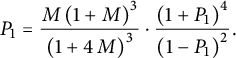 $$\begin{align*}P_1 ={\frac {M \left(1+ M \right) ^ {3} }{ \left(1+ 4\,M \right) ^{3}}}\cdot\frac{\left(1+ P_1 \right) ^{4}}{\left( 1-P_1 \right) ^{2}}. \end{align*}$$
Finally, we define
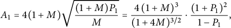 $$\begin{align*}A_1= 4 (1+M) \sqrt{\frac{(1+M)P_1}M} = \frac{4\,(1+M)^3}{(1+4M)^{3/2}} \cdot \frac {(1+P_1)^2}{1-P_1 }, \end{align*}$$
which has degree $8$
above
$8$
above $\mathbb {Q}(M)$
and degree
$\mathbb {Q}(M)$
and degree $16$
above
$16$
above $\mathbb {Q}(t)$
. Between
$\mathbb {Q}(t)$
. Between $\mathbb {Q}(M)$
and
$\mathbb {Q}(M)$
and $\mathbb {Q}(M,A_1)=\mathbb {Q}(t, A_1)$
, there are three extensions of
$\mathbb {Q}(M,A_1)=\mathbb {Q}(t, A_1)$
, there are three extensions of $\mathbb {Q}(M)$
of degree
$\mathbb {Q}(M)$
of degree $2$
, respectively, generated by
$2$
, respectively, generated by $\sqrt {1+4M}$
,
$\sqrt {1+4M}$
, $\sqrt {1-4M^2}$
, and
$\sqrt {1-4M^2}$
, and $\sqrt {(1+4M)(1-4M^2)}$
. We shall consider, in particular, a generator of
$\sqrt {(1+4M)(1-4M^2)}$
. We shall consider, in particular, a generator of $\mathbb {Q}(\sqrt {1+4M})$
, denoted by N, defined by
$\mathbb {Q}(\sqrt {1+4M})$
, denoted by N, defined by $N=\mathcal O(t)$
and
$N=\mathcal O(t)$
and
 $$ \begin{align} \qquad N = t\, \frac{N^4-2N^3+6N^2-2N+1}{(1-N)^2}, \quad \mbox{or equivalently} \quad N=M(1-N)^2. \hspace{-20pt}\end{align} $$
Figure 3 gives a complete description of $\mathbb {Q}(t,A_1)$
and its subfields. The series denoted by
$\mathbb {Q}(t,A_1)$
and its subfields. The series denoted by $P_2$
is the only solution of
$P_2$
is the only solution of
 $$\begin{align*}P_2^4 - (1+4M)^3P_2^2 + 4M(1+ M)^3(1+4M)^3 =0, \end{align*}$$
satisfying $P_2=1+\mathcal {O}(t)$
. It is related to M,
$P_2=1+\mathcal {O}(t)$
. It is related to M, $P_1$
, and
$P_1$
, and $A_1$
by
$A_1$
by
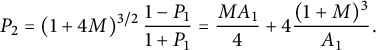 $$ \begin{align} P_2= (1+4M)^{3/2} \, \frac{1-P_1}{1+P_1} = \frac{M A_1}{4} + 4 \frac{(1+M)^3}{A_1}. \end{align} $$
Theorem 6.1 The generating function $C(x,y)$
of walks with steps in
$C(x,y)$
of walks with steps in $\{\rightarrow , \uparrow , \swarrow , \nearrow , \leftarrow , \downarrow\}$
starting from
$\{\rightarrow , \uparrow , \swarrow , \nearrow , \leftarrow , \downarrow\}$
starting from $(0,0)$
and avoiding the negative quadrant is algebraic of degree
$(0,0)$
and avoiding the negative quadrant is algebraic of degree $256$
. It is given by the following equation:
$256$
. It is given by the following equation:
 $$\begin{align*}(1-t(x+y +xy+\bar x\bar y+\bar x+\bar y)) C(x,y)&=1 -t\bar y(1+\bar x) C_-(\bar x)\\ &\quad -t\bar x(1+\bar y) C_-(\bar y)- t \bar x\bar y C_{0,0}, \end{align*}$$
where $C_{0,0}$
is algebraic of degree
$C_{0,0}$
is algebraic of degree $16$
and
$16$
and $C_-(x)$
is algebraic of degree
$C_-(x)$
is algebraic of degree $64$
. These series can be expressed in terms of the series M, N, and
$64$
. These series can be expressed in terms of the series M, N, and $A_1$
defined above. Indeed,
$A_1$
defined above. Indeed,
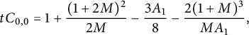 $$ \begin{align} t C_{0,0}= 1+ \frac{(1+2M)^2}{2M} -\frac{3A_1}8 - \frac{2(1+M)^3}{M A_1}, \end{align} $$
and
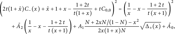 $$ \begin{align} &\left(2t (1+\bar x) C_-(x)+\bar x +1+x-\frac{1+2t}{t(1+x)} +t C_{0,0}\right)^2= \left( \frac 1 x-x-{\frac {1+2\,t}{t \left( x+1 \right) }}\right)^2 \nonumber\\ &\qquad+\tilde A_2 \left( \frac 1 x-x-{\frac {1+2\,t}{t \left( x+1 \right) }}\right)+A_1 \frac{N+2xN/(1-N)-x^2}{2x(1+x)N}\sqrt{\Delta_+(x)}+\tilde A_0, \end{align} $$
where $\Delta _+(x)$
is the following polynomial in x:
$\Delta _+(x)$
is the following polynomial in x:
 $$ \begin{align} \Delta_+(x)=1- \frac{2N(1+N^2)}{(1-N)^2} x +N^2 x^2, \end{align} $$
and $\tilde A_2$
and
$\tilde A_2$
and $\tilde A_0$
are algebraic series of respective degree
$\tilde A_0$
are algebraic series of respective degree $8$
and
$8$
and $16$
, both in
$16$
, both in $\mathbb {Q}(t, A_1)$
:
$\mathbb {Q}(t, A_1)$
:
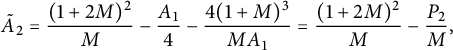 $$\begin{align*}\tilde A_2= \frac{(1+2M)^2}M -\frac{A_1}4 - \frac{4(1+M)^3}{M A_1} = \frac{(1+2M)^2}M - \frac{P_2}{M}, \end{align*}$$
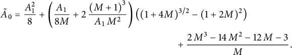 $$ \begin{align*} \tilde A_0= \frac{A_1^{2}}8 + \left({\frac {A_1\, }{8M}}+2\,{ \frac { \left( M+1 \right) ^{3} }{A_1\,{M} ^{2}}} \right)& \left((1+4M)^{3/2}-(1+2M)^2\right) \\ &\qquad\qquad +{\frac {2\,{M}^{3}-14\,{M}^ {2}-12\,M-3}{M}}. \end{align*} $$
The generating function $D(x)$
of walks ending on the diagonal is algebraic of degree
$D(x)$
of walks ending on the diagonal is algebraic of degree $64$
, given by
$64$
, given by
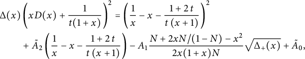 $$ \begin{align} \Delta(x)& \left(xD(x)+ \frac{1}{t(1+x)}\right)^2= \left( \frac 1 x-x-{\frac {1+2\,t}{t \left( x+1 \right) }}\right)^2 \nonumber \\ &+\tilde A_2 \left( \frac 1 x-x-{\frac {1+2\,t}{t \left( x+1 \right) }}\right)-A_1 \frac{N+2xN/(1-N)-x^2}{2x(1+x)N} \sqrt{\Delta_+(x)}+\tilde A_0, \end{align} $$
with the above values of $\Delta _+(x), \tilde A_0, A_1, \tilde A_2$
, and
$\Delta _+(x), \tilde A_0, A_1, \tilde A_2$
, and
 $$ \begin{align} \Delta(x)= (1-t(x+\bar x))^2-4t^2\bar x(1+x)^2. \end{align} $$
For walks ending at a prescribed position, we obtain the following result.
Corollary 6.2 Let us define $A_1$
as above. For any
$A_1$
as above. For any $(i,j)\in \mathcal {C}$
, the generating function of walks avoiding the negative quadrant and ending at
$(i,j)\in \mathcal {C}$
, the generating function of walks avoiding the negative quadrant and ending at $(i,j)$
is algebraic of degree (at most)
$(i,j)$
is algebraic of degree (at most) $16$
and belongs to
$16$
and belongs to $\mathbb {Q}(t, A_1)$
.
$\mathbb {Q}(t, A_1)$
.
The first example is provided by the expression of $C_{0,0}$
in (6.3). A simpler one is
$C_{0,0}$
in (6.3). A simpler one is
 $$ \begin{align} t C_{-1,0} =\frac{A_1}4-1. \end{align} $$
Now, for the generating function C(1,1) that counts all walks avoiding the negative quadrant, it follows from Theorem 6.1 that
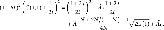 $$\begin{align*}(1-6t)^2 \left( C(1,1) + \frac 1 {2t} \right)^2&= \left( {\frac {1+2\,t}{2t }}\right)^2 -\tilde A_2 {\frac {1+2\,t}{2t }}\\&\quad +A_1 \frac{N+2N/(1-N)-1}{4N}\sqrt{\Delta_+(1)}+\tilde A_0. \end{align*}$$
Upon noticing that $\Delta _+(1)=(1-N)^2(1-4M^2)$
, one sees that the right-hand side belongs to
$\Delta _+(1)=(1-N)^2(1-4M^2)$
, one sees that the right-hand side belongs to $\mathbb {Q}(t, A_1)$
, and could thus be expected to have degree
$\mathbb {Q}(t, A_1)$
, and could thus be expected to have degree $16$
(which would give an expected degree
$16$
(which would give an expected degree $32$
for
$32$
for $C(1,1)$
). However, the right-hand side belongs to
$C(1,1)$
). However, the right-hand side belongs to $\mathbb {Q}(t,A_1^2)$
and has degree
$\mathbb {Q}(t,A_1^2)$
and has degree $8$
only, as made explicit in the following corollary. Details of the derivation are available in our Maple session.
$8$
only, as made explicit in the following corollary. Details of the derivation are available in our Maple session.
Corollary 6.3 The generating function $C(1,1)$
counting by their length all walks with steps in
$C(1,1)$
counting by their length all walks with steps in $\mathcal S$
avoiding the negative quadrant is algebraic of degree
$\mathcal S$
avoiding the negative quadrant is algebraic of degree $16$
over
$16$
over $\mathbb {Q}(t)$
, and of degree
$\mathbb {Q}(t)$
, and of degree $2$
over
$2$
over $\mathbb {Q}(t,A_1^2)$
. More precisely,
$\mathbb {Q}(t,A_1^2)$
. More precisely,
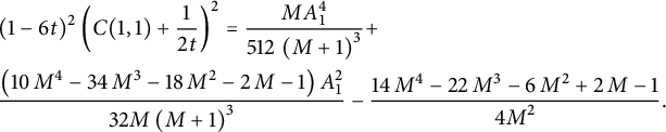 $$ \begin{align} &\qquad (1-6t)^2 \left( C(1,1) + \frac 1 {2t} \right)^2= {\frac {M A_1^{4}}{512\, \left( M+1 \right) ^{3}}}+ \hspace{-20pt}\nonumber\\ &\qquad {\frac { \left( 10\,{M}^{4}-34\,{M}^{3}-18\,{M}^{2}-2\,M-1 \right) A_1 ^{2}}{32M \left( M+1 \right) ^{3}}} -{\frac {14\,{M}^{4}-22\,{M}^{3} -6\,{M}^{2}+2\,M-1}{{4M}^{2}}}. \hspace{-20pt}\end{align} $$
It has radius $1/6$
, with a unique dominant singularity at
$1/6$
, with a unique dominant singularity at $1/6$
. As t approaches this point,
$1/6$
. As t approaches this point,
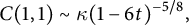 $$\begin{align*}C(1,1) \sim \kappa (1-6t)^{-5/8}, \end{align*}$$
with
 $$\begin{align*}\kappa= 2^{1/4} 3^{9/8} (\sqrt 2-1). \end{align*}$$
Hence, the number of walks of length n avoiding the negative quadrant satisfies
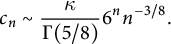 $$\begin{align*}c_n \sim \frac {\kappa} {\Gamma(5/8)} 6^{n} n^{-3/8}. \end{align*}$$
Harmonic function
We have also derived the counterpart of Corollary 1.4, that is, a harmonic function on $\mathcal {C}$
associated with the double Kreweras step set
$\mathcal {C}$
associated with the double Kreweras step set $\mathcal S=\mathcal S^*=\{\rightarrow , \nearrow , \uparrow , \leftarrow , \swarrow , \downarrow \}$
. We still have an asymptotic behavior of the form (1.7), with the factor
$\mathcal S=\mathcal S^*=\{\rightarrow , \nearrow , \uparrow , \leftarrow , \swarrow , \downarrow \}$
. We still have an asymptotic behavior of the form (1.7), with the factor $3^n$
replaced of course by
$3^n$
replaced of course by $6^n$
, and without any periodicity condition. We do not give here all details of the numbers
$6^n$
, and without any periodicity condition. We do not give here all details of the numbers $H_{i,j}$
, but simply the values of
$H_{i,j}$
, but simply the values of
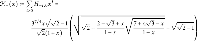 $$ \begin{align*} \mathcal H_-(x)&:=\sum_{i>0} H_{-i,0} x^i= \\ &\qquad\frac{3^{7/4} x\sqrt{\sqrt 2 -1}}{\sqrt 2 (1+x) } \left( \sqrt{\sqrt 2 + \frac{2-\sqrt 3 +x}{1-x}\sqrt{\frac{7+4\sqrt 3 -x}{1-x}}} -\sqrt{\sqrt 2-1}\right) \end{align*} $$
and
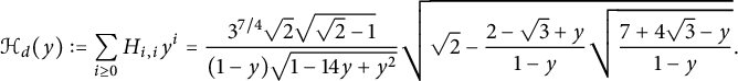 $$\begin{align*}\mathcal H_d(y):=\sum_{i\ge 0} H_{i,i}y^i = \frac{3^{7/4}\sqrt 2 \sqrt{\sqrt 2 -1}}{(1-y)\sqrt{1-14y+y^2}} \sqrt{\sqrt 2 - \frac{2-\sqrt 3 +y}{1-y}\sqrt{\frac{7+4\sqrt 3-y}{1-y}}}. \end{align*}$$
The proof is analogous to Kreweras’ case, and in fact a bit easier since the model $\mathcal S$
is aperiodic. Once again, details of the calculations can be found in our Maple session. The number of quadrant
$\mathcal S$
is aperiodic. Once again, details of the calculations can be found in our Maple session. The number of quadrant $\mathscr S$
-walks of length n going from
$\mathscr S$
-walks of length n going from $(0,0)$
to
$(0,0)$
to $(i,j)$
in the first quadrant is now asymptotic to
$(i,j)$
in the first quadrant is now asymptotic to $h_{i,j} 6^n n^{-5/2} / \Gamma (-3/2)$
, with
$h_{i,j} 6^n n^{-5/2} / \Gamma (-3/2)$
, with
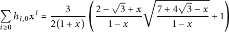 $$\begin{align*}\sum_{i\ge 0} h_{i,0} x^i=\frac 3 {2(1+x)} \left( \frac{2-\sqrt 3 +x}{1-x} \sqrt{\frac{7+4\sqrt 3 -x}{1-x}} +1 \right) \end{align*}$$
(and in this case uniqueness of the positive harmonic function is proved [Reference Bouaziz, Mustapha and Sifi7]).
6.2 Proofs for double Kreweras steps
Proof of Theorem 6.1
Proof. The first equation of the theorem is of course the basic functional equation (2.4). The functional equations (2.8) and (2.12) defining $D(y)$
and
$D(y)$
and $U(x,y)$
read
$U(x,y)$
read
 $$ \begin{align} (1-t(y+\bar y)) D(y) =1 -t\bar y D_0+2t(1+\bar y)U(0,y) -2t\bar y U_{0,0}, \end{align} $$
 $$ \begin{align*} &2xy(1-t(\bar x\bar y+x+y+\bar x+\bar y+xy)) U(x,y) = \\ &\phantom{2xy(1-t(\bar x\bar y} y+ y\left(t(y+\bar y) +2tx(1+y)-1\right) D(y) -2t(1+x) U(x,0) - t D_0. \end{align*} $$
The invariants of Proposition 3.3 are
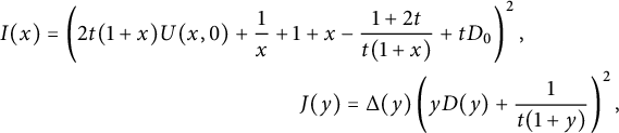 $$ \begin{align*} I(x)&=\left( 2t(1+x)U(x,0)+\frac 1 {x}+1+x -\frac {1+2t} {t(1+x)} + tD_0\right)^2, \\ &\phantom{2t(1+x)U(x,0)+\frac 1 {x}+1+x } J(y)=\Delta(y)\left(yD(y)+ \frac 1 {t(1+y)} \right)^2, \end{align*} $$
with $\Delta $
defined by (6.7). Note that they have now poles at
$\Delta $
defined by (6.7). Note that they have now poles at $0$
and at
$0$
and at $-1$
. The rational invariants
$-1$
. The rational invariants $I_0,J_0$
are given by Table 3:
$I_0,J_0$
are given by Table 3:
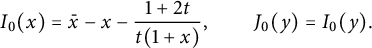 $$\begin{align*}I_0(x)= \bar x -x -\frac{1+2t}{t(1+x)}, \qquad J_0(y)=I_0(y). \end{align*}$$
They satisfy
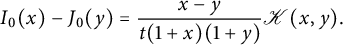 $$ \begin{align} I_0(x)-J_0(y)= \frac{x-y}{t(1+x)(1+y)} \mathscr K(x,y). \end{align} $$
The invariants (2.24) related to quadrant walks with steps in $\mathscr S$
are
$\mathscr S$
are
 $$\begin{align*}I_1(x)= t(1+x)\mathscr Q(x,0) -\frac{x-t-tx^2}{t(1+x)}, \qquad J_1(y)=-t(1+y)\mathscr Q(0,y)+t\mathscr Q_{0,0}-\bar y. \end{align*}$$
They satisfy
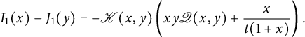 $$ \begin{align} I_1(x)-J_1(y)= -\mathscr K(x,y) \left( xy\mathscr Q(x,y)+ \frac x{t(1+x)}\right). \end{align} $$
Applying the invariant lemma
Again, we want to combine these three pairs of invariants to form a pair satisfying the condition of Lemma 2.6. As in the previous section, we look for a polynomial combination of $I(x), I_0(x)$
, and
$I(x), I_0(x)$
, and $I_1(x)$
that, at least, has no pole at
$I_1(x)$
that, at least, has no pole at $x=0$
nor at
$x=0$
nor at $x=-1$
. We first eliminate poles at
$x=-1$
. We first eliminate poles at $0$
using
$0$
using $I_0(x)$
, and then poles at
$I_0(x)$
, and then poles at $-1$
using
$-1$
using $I_1(x)$
. We are thus led to consider
$I_1(x)$
. We are thus led to consider
 $$\begin{align*}\tilde I(x):= I(x) -I_0(x)^2 -A_2I_0(x)-A_1 I_1(x), \end{align*}$$
with
 $$ \begin{align} A_2=2(1+tD_0+2tU_{0,0}), \qquad A_1= 4(1+tU_{0,0}), \end{align} $$
which indeed has no pole at $x=0$
nor at
$x=0$
nor at $x=-1$
. Let us define accordingly
$x=-1$
. Let us define accordingly
 $$\begin{align*}\tilde J(y)= J(y) -J_0(y)^2 -A_2J_0(y)-A_1 J_1(y), \end{align*}$$
and examine whether the ratio $(\tilde I(x)-\tilde J(y))/\mathscr K(x,y)$
is a multiple of
$(\tilde I(x)-\tilde J(y))/\mathscr K(x,y)$
is a multiple of $xy$
. We proceed as in the previous section. Denoting by
$xy$
. We proceed as in the previous section. Denoting by $\operatorname {\mathrm {Rat}}$
,
$\operatorname {\mathrm {Rat}}$
, $\operatorname {\mathrm {Rat}}_0$
, and
$\operatorname {\mathrm {Rat}}_0$
, and $\operatorname {\mathrm {Rat}}_1$
the right-hand sides of (3.7), (6.11), and (6.12), the expression (5.16) of
$\operatorname {\mathrm {Rat}}_1$
the right-hand sides of (3.7), (6.11), and (6.12), the expression (5.16) of $(\tilde I(x)-\tilde J(y))/\mathscr K(x,y)$
still holds (because
$(\tilde I(x)-\tilde J(y))/\mathscr K(x,y)$
still holds (because $\tilde I(x)$
and
$\tilde I(x)$
and $\tilde J(y)$
have the same form for both models). In order to see that this ratio is indeed a multiple of x, we need to inject (6.10). Proving that it is a multiple of y requires no additional information. We conclude that the pair
$\tilde J(y)$
have the same form for both models). In order to see that this ratio is indeed a multiple of x, we need to inject (6.10). Proving that it is a multiple of y requires no additional information. We conclude that the pair $(\tilde I(x), \tilde J(x))$
is constant, equal to
$(\tilde I(x), \tilde J(x))$
is constant, equal to $(A_0, A_0)$
for some series
$(A_0, A_0)$
for some series $A_0$
that depends on t only.
$A_0$
that depends on t only.
Recall that $I_1(x)$
is expressed in terms of the generating function
$I_1(x)$
is expressed in terms of the generating function $\mathscr Q(x,0)$
of quadrant walks with double Kreweras steps. This series is known, and we obtain from Proposition 15 in [Reference Bousquet-Mélou and Mishna10]
$\mathscr Q(x,0)$
of quadrant walks with double Kreweras steps. This series is known, and we obtain from Proposition 15 in [Reference Bousquet-Mélou and Mishna10]
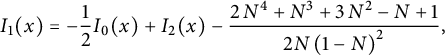 $$\begin{align*}I_1(x)= -\frac 1 2 I_0(x) + I_2(x) -{\frac {2\,{N}^{4}+{N}^{3}+3\,{N}^{2}-N+1}{2N \left(1- N \right) ^{2}}}, \end{align*}$$
where N is defined by (6.1) (this series is denoted by Z in [Reference Bousquet-Mélou and Mishna10]) and
 $$\begin{align*}I_2(x):= \frac{N+2xN/(1-N)-x^2}{2x(1+x)N}\sqrt{\Delta_+(x)}, \end{align*}$$
with $ \Delta _+(x)$
given by (6.5). In what follows, we use
$ \Delta _+(x)$
given by (6.5). In what follows, we use $I_2(x)$
rather than
$I_2(x)$
rather than $I_1(x)$
. That is, we rewrite the identity
$I_1(x)$
. That is, we rewrite the identity $\tilde I(x)=A_0$
, which reads
$\tilde I(x)=A_0$
, which reads
 $$\begin{align*}I(x)= I_0(x)^2 +A_2I_0(x)+A_1 I_1(x)+A_0 \end{align*}$$
as
 $$ \begin{align} I(x)= I_0(x)^2 +\tilde A_2I_0(x)+A_1 I_2(x)+\tilde A_0, \end{align} $$
where the two new series $\tilde A_2$
and
$\tilde A_2$
and $\tilde A_0$
are
$\tilde A_0$
are
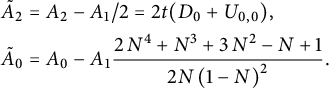 $$ \begin{align} \tilde A_2&= A_2-A_1/2=2t(D_0+U_{0,0}), \\ \tilde A_0&=A_0-A_1 {\frac {2\,{N}^{4}+{N}^{3}+3\,{N}^{2}-N+1}{2N \left(1- N \right) ^{2}}}. \nonumber \end{align} $$
Similarly, we find that the quadrant invariant $J_1(y)$
is given by
$J_1(y)$
is given by
 $$\begin{align*}J_1(y)= -\frac 1 2 J_0(y) - I_2(y) -{\frac {2\,{N}^{4}+{N}^{3}+3\,{N}^{2}-N+1}{2N \left(1- N \right) ^{2}}}, \end{align*}$$
and write
 $$ \begin{align} J(y)= J_0(y)^2 +\tilde A_2J_0(y)-A_1 I_2(y)+\tilde A_0, \end{align} $$
with the above values of $\tilde A_2$
and
$\tilde A_2$
and $ \tilde A_0$
.
$ \tilde A_0$
.
This gives the expressions (6.4) and (6.6) announced in Theorem 6.1, which are those of $I(x)$
and
$I(x)$
and $J(x)$
. However, we still need to determine the three series
$J(x)$
. However, we still need to determine the three series $\tilde A_0, A_1$
, and
$\tilde A_0, A_1$
, and $\tilde A_2$
.
$\tilde A_2$
.
The series
$\tilde A_0, A_1$
, and
$\tilde A_2$


We cannot follow exactly the same approach as in the previous section, where we had written all invariants as polynomials in $I_1(x)$
using the identity (5.18) (it is still possible to write
$I_1(x)$
using the identity (5.18) (it is still possible to write $I(x)$
as a rational function of
$I(x)$
as a rational function of $I_1(x)$
; see Section 9.1). Indeed, the counterpart of this identity relates now
$I_1(x)$
; see Section 9.1). Indeed, the counterpart of this identity relates now $I_0$
and
$I_0$
and $I_2$
, and is no longer linear in
$I_2$
, and is no longer linear in $I_0$
:
$I_0$
:
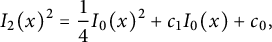 $$\begin{align*}I_2(x)^2= \frac{1}4 I_0(x)^2+ c_1 I_0(x) + c_0, \end{align*}$$
with
 $$\begin{align*}c_1= \frac{1+N+N^2-N^3}{2N(1-N)^2} \qquad \mbox{and} \qquad c_0={\frac { \left( N^{2}+1 \right) \left( 4\,N^{4}-9\,N^{3}+ 13\,N^{2}-N+1 \right) }{4 N^{2}\left( 1-N \right) ^{3}}}. \end{align*}$$
However, compare the expressions (6.14) and (6.16) of $I(x)$
and
$I(x)$
and $J(y)$
, and recall that
$J(y)$
, and recall that $J_0(y)=I_0(y)$
. This, as well as the above expression of
$J_0(y)=I_0(y)$
. This, as well as the above expression of $I_2(x)^2$
, suggests to form the product
$I_2(x)^2$
, suggests to form the product $I(x) J(x)$
, which will be a polynomial in
$I(x) J(x)$
, which will be a polynomial in $I_0(x)$
:
$I_0(x)$
:
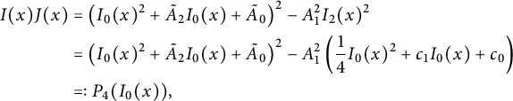 $$ \begin{align*} I(x) J(x)&= \left( I_0(x)^2 +\tilde A_2I_0(x)+\tilde A_0\right)^2-A_1^2 I_2(x)^2 \\ &= \left( I_0(x)^2 +\tilde A_2I_0(x)+\tilde A_0\right)^2-A_1^2 \left(\frac{1}4 I_0(x)^2+ c_1 I_0(x) + c_0\right) \\ & =: P_4(I_0(x)), \end{align*} $$
where
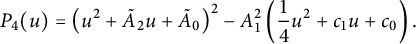 $$\begin{align*}P_4(u)= \left( u^2 +\tilde A_2u+\tilde A_0\right)^2-A_1^2 \left(\frac{1}4 u^2+ c_1 u + c_0\right). \end{align*}$$
We can now apply the same ideas as in the previous case. The product $I(x)J(x)$
vanishes:
$I(x)J(x)$
vanishes:
-
• when x is one of the two roots of
$\Delta (x)$
, denoted by
$X_+$
and
$X_-$
, that are finite at
$t=0$
; -
• when
$x=X=t+3t^3+ \mathcal O(t^4)$
is the (only) root of
$I(x)$
lying in
$\mathbb {Q}[[t]]$
, that is,
$$\begin{align*}X= t\,\frac{1+X}{1+2t}\left( 2t (1+X) C_-(X)+1 +X+X^2 +t XC_{0,0}\right). \end{align*}$$


The values $I_0(X_\pm )$
are found to be the two roots of
$I_0(X_\pm )$
are found to be the two roots of
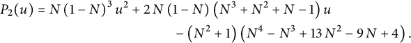 $$ \begin{align*} P_2(u)= N \left( 1-N \right) ^{3}u^{2}&+2\,N \left( 1-N \right) \left( {N}^{3}+{N}^{2}+N-1 \right) u\\ &\qquad\quad- \left( {N}^{2}+1 \right) \left( {N}^{4}-{N}^{3}+13\,{N}^{2}-9\,N+4 \right). \end{align*} $$
(This polynomial should not be mixed up with the series $P_2$
of (6.2)!) They expand as
$P_2$
of (6.2)!) They expand as
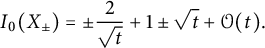 $$\begin{align*}I_0(X_\pm)=\pm \frac 2{\sqrt t} + 1 \pm \sqrt t +\mathcal{O}(t). \end{align*}$$
Now, the series $I_0(X)=-1+\mathcal {O}(t)$
is also a root of
$I_0(X)=-1+\mathcal {O}(t)$
is also a root of $P_4(u)$
, distinct from
$P_4(u)$
, distinct from $I_0(X_\pm )$
, and in fact is even a double root of
$I_0(X_\pm )$
, and in fact is even a double root of $P_4$
(as before, one has to check that
$P_4$
(as before, one has to check that $I^{\prime }_0(X)\not = 0$
). Hence, we have the following factorization:
$I^{\prime }_0(X)\not = 0$
). Hence, we have the following factorization:
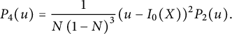 $$\begin{align*}P_4(u)=\frac 1{N\left( 1-N \right) ^{3}} (u-I_0(X))^2 P_2(u). \end{align*}$$
We now equate the coefficients of $u^3, \ldots , u^0$
in both sides of this identity. From the coefficients of
$u^3, \ldots , u^0$
in both sides of this identity. From the coefficients of $u^3$
, we obtain
$u^3$
, we obtain
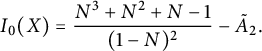 $$\begin{align*}I_0(X)= \frac{N^3+N^2+N-1}{(1-N)^2}-\tilde A_2. \end{align*}$$
We then replace every occurrence of $I_0(X)$
by this expression. The coefficients of
$I_0(X)$
by this expression. The coefficients of $u^2$
give
$u^2$
give
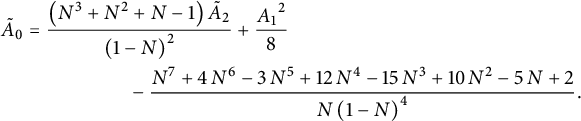 $$ \begin{align} \tilde A_0&= {\frac { \left( {N}^{3}+{N}^{2}+N-1 \right) {\tilde A_2}}{ \left( 1-N \right) ^{2}}} +\frac{{A_1}^{2}}8 \nonumber\\ &\qquad\qquad\quad-{\frac {{N}^{7}+4\,{N}^{6}-3\,{N}^ {5}+12\,{N}^{4}-15\,{N}^{3}+10\,{N}^{2}-5\,N+2}{N \left( 1-N \right) ^{4}}}. \end{align} $$
We proceed with the coefficients of $u^1$
, after replacing every occurrence of
$u^1$
, after replacing every occurrence of $\tilde A_0$
by the above expression. This gives
$\tilde A_0$
by the above expression. This gives
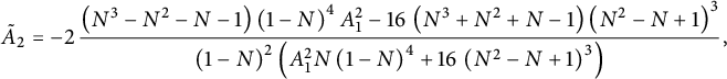 $$ \begin{align} \tilde A_2= -2\,{\frac { \left( {N}^{3}-{N}^{2}-N-1 \right) \left( 1-N \right) ^ {4}A_1^{2}-16\, \left( {N}^{3}+{N}^{2}+N-1 \right) \left( {N}^ {2}-N+1 \right) ^{3}}{ \left( 1-N \right) ^{2} \left( A_1^{2}N \left( 1-N \right) ^{4}+16\, \left( {N}^{2}-N+1 \right) ^{3} \right) }} , \end{align} $$
and we finally derive by comparing constant terms that
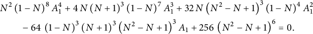 $$ \begin{align} & {N}^{2} \left( 1-N \right) ^{8}A_1^{4} +4\,N \left( N+1 \right) ^{3} \left( 1-N \right) ^{7}A_1^{3} +32\,N \left( {N}^{2}-N+1 \right) ^{3} \left( 1-N \right) ^{4}A_1^{2}\nonumber\\ &\qquad -64\, \left( 1-N \right) ^{3} \left( N+1 \right) ^{3} \left( {N}^{2}-N+1 \right) ^{3}A_1+256\, \left( {N}^{2}-N +1 \right) ^{6} =0. \end{align} $$
One can now check, using this equation and the first terms $A_1=4+4t^2+\mathcal {O}(t^3)$
, that
$A_1=4+4t^2+\mathcal {O}(t^3)$
, that $A_1$
is indeed the series described at the beginning of the section, and that the values of
$A_1$
is indeed the series described at the beginning of the section, and that the values of $\tilde A_2$
and
$\tilde A_2$
and $\tilde A_0$
given in the theorem in terms of the series M and
$\tilde A_0$
given in the theorem in terms of the series M and $A_1$
coincide with those derived from (6.18) and (6.17).
$A_1$
coincide with those derived from (6.18) and (6.17).
It also follows from (6.13) and (6.15) that
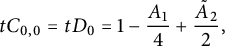 $$\begin{align*}tC_{0,0}=tD_0=1-\frac{A_1}4 + \frac {\tilde A_2}2 , \end{align*}$$
and the expression (6.3) can again be checked using (6.18) and (6.19).
Degrees
From the identities in this theorem, it follows that $C_-(x,0)$
and
$C_-(x,0)$
and $D(x)$
have degree at most
$D(x)$
have degree at most $16\times 4=64$
above
$16\times 4=64$
above $\mathbb {Q}(t,x)$
. To prove that this bound is tight, we compute by elimination the minimal polynomials of
$\mathbb {Q}(t,x)$
. To prove that this bound is tight, we compute by elimination the minimal polynomials of $C_-(2,0)$
and
$C_-(2,0)$
and $D(2)$
. We proceed similarly for the degree of
$D(2)$
. We proceed similarly for the degree of $C(x,y)$
, for which the natural upper bound is
$C(x,y)$
, for which the natural upper bound is $16\times 4\times 4=256$
. In this case, we specialize not only x and y, but also t, in such a way that
$16\times 4\times 4=256$
. In this case, we specialize not only x and y, but also t, in such a way that $xyt<1/6$
, which guarantees the convergence of all series under consideration.
$xyt<1/6$
, which guarantees the convergence of all series under consideration.
Remark 6.4 It may be interesting for some readers to know how one can derive from the polynomial equation (6.19) the description of the series $A_1$
, and of the subfields of
$A_1$
, and of the subfields of $\mathbb {Q}(t,A_1)$
, given at the beginning of the section (see Figure 3). This is fully documented in the Maple session that accompanies this paper, but here are a few details.
$\mathbb {Q}(t,A_1)$
, given at the beginning of the section (see Figure 3). This is fully documented in the Maple session that accompanies this paper, but here are a few details.
Recall that the series N arises from the earlier paper [Reference Bousquet-Mélou and Mishna10]. The first step is to investigate the subextensions of $\mathbb {Q}(t,N)$
and to discover the series M. This can be done, for instance, using the Subfields command.
$\mathbb {Q}(t,N)$
and to discover the series M. This can be done, for instance, using the Subfields command.
Then, it is easy to prove, by elimination of N, that $A_1$
has degree
$A_1$
has degree $16$
over
$16$
over $\mathbb {Q}(t)$
. The idea of introducing the generator
$\mathbb {Q}(t)$
. The idea of introducing the generator $P_1$
comes by looking at the denominator of
$P_1$
comes by looking at the denominator of $\tilde A_2$
in (6.18), and observing that the defining equation (6.19) of
$\tilde A_2$
in (6.18), and observing that the defining equation (6.19) of $A_1$
can also be written in the form:
$A_1$
can also be written in the form:
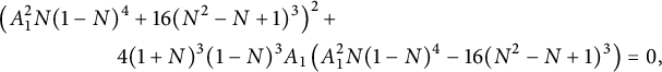 $$ \begin{align*} &\left(A_1^2N(1 - N)^4 + 16(N^2 - N + 1)^3\right)^2+ \\ &\phantom{A_1^2N(1 - N)^4} 4(1+N )^3(1 - N)^3A_1 \left(A_1^2N(1 - N)^4 - 16(N^2 - N + 1)^3\right)=0, \end{align*} $$
or, in terms of M,
 $$\begin{align*}\left(M A_1^2 + 16 (1+M )^3\right)^2 + 4 A_1 (1+4 M )^{3/2} \left(M A_1^2 - 16 (1+M )^3\right)=0. \end{align*}$$
Once $P_1$
is thus defined, one explores the subfields of
$P_1$
is thus defined, one explores the subfields of $\mathbb {Q}(t,A_1)$
using the Subfields command.
$\mathbb {Q}(t,A_1)$
using the Subfields command.
We now consider number of walks ending at $(i,j)$
.
$(i,j)$
.
Proof of Corollary 6.2
This model is aperiodic. The right-hand side of (6.4) is a (Laurent) series in x with coefficients in $\mathbb {Q}(t,A_1)$
, with first term
$\mathbb {Q}(t,A_1)$
, with first term $1/x^2$
. So its square root is a Laurent series in x, starting with
$1/x^2$
. So its square root is a Laurent series in x, starting with $1/x$
, with coefficients in
$1/x$
, with coefficients in $\mathbb {Q}(t,A_1)$
again. This proves the corollary for the coefficients of
$\mathbb {Q}(t,A_1)$
again. This proves the corollary for the coefficients of $U(x,0)$
, that is, for the series
$U(x,0)$
, that is, for the series $C_{i,0}$
with
$C_{i,0}$
with $i<0$
. The value of
$i<0$
. The value of $C_{-1,0}$
given in (6.8) comes directly from (6.13).
$C_{-1,0}$
given in (6.8) comes directly from (6.13).
A similar argument, based on (6.6), proves the result for the series $C_{i,i}$
. We then prove the corollary for the points
$C_{i,i}$
. We then prove the corollary for the points $(i,i+1)$
, by induction on
$(i,i+1)$
, by induction on $i\ge 0$
, by writing
$i\ge 0$
, by writing

We finally prove it for all points $(i,j)$
with
$(i,j)$
with $j\ge i$
by induction on
$j\ge i$
by induction on $2j-i\ge 0$
, using
$2j-i\ge 0$
, using
 $$\begin{align*}C_{i,j-1}= t(C_{i,j-2}+C_{i,j}+C_{i-1,j-1}+ C_{i+1,j-1} +C_{i-1,j-2} +C_{i+1,j}).\\[-34pt] \end{align*}$$
7 A D-algebraic model
Let us now consider the $6$
th model of Table 1, with step polynomial
$6$
th model of Table 1, with step polynomial $S(x,y)= x+\bar x +y+\bar y +xy$
. The companion model is given by
$S(x,y)= x+\bar x +y+\bar y +xy$
. The companion model is given by $\mathscr S(x,y)= x+\bar x +xy +\bar x \bar y +y$
. In this case, there are no rational
$\mathscr S(x,y)= x+\bar x +xy +\bar x \bar y +y$
. In this case, there are no rational $\mathscr S$
-invariants, but there exists a pair of quadrant invariants of the form (2.24) (see Table 4), namely
$\mathscr S$
-invariants, but there exists a pair of quadrant invariants of the form (2.24) (see Table 4), namely $(I_1(x), J_1(y))$
, with
$(I_1(x), J_1(y))$
, with
 $$ \begin{align} \qquad I_1(x) = t \mathscr Q(x,0)+ \bar x, \qquad J_1(y) = -t(1+y)\mathscr Q(0,y)+t\mathscr Q_{0,0} + \frac{y(1-ty)}{t(1+y)}. \hspace{-20pt}\end{align} $$
This pair satisfies
 $$\begin{align*}I_1(x) -J_1(y) =- \mathscr K(x,y) \left(xy\mathscr Q(x,y)+\frac y{t(1+y)} \right). \end{align*}$$
The series $\mathscr Q(x,y)$
is known to be D-algebraic, and admits an explicit expression in terms of elliptic functions [Reference Bernardi, Bousquet-Mélou and Raschel2, Theorem 5.7]. Our approach relates
$\mathscr Q(x,y)$
is known to be D-algebraic, and admits an explicit expression in terms of elliptic functions [Reference Bernardi, Bousquet-Mélou and Raschel2, Theorem 5.7]. Our approach relates $C(x,y)$
to this series.
$C(x,y)$
to this series.
Table 4: $\mathscr S$
-decoupling of
$\mathscr S$
-decoupling of $xy$
by f and g for infinite group models. The associated invariants
$xy$
by f and g for infinite group models. The associated invariants $I_1(x), J_1(y)$
defined by (2.24) are D-algebraic.
$I_1(x), J_1(y)$
defined by (2.24) are D-algebraic.
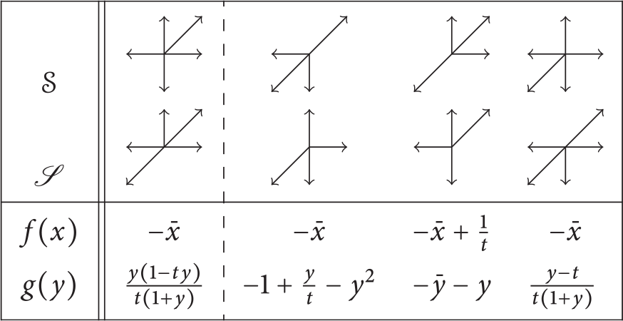
7.1 Generating functions
Theorem 7.1 Let $I_1(x)$
and
$I_1(x)$
and $J_1(y)$
be defined as above. The generating function
$J_1(y)$
be defined as above. The generating function $C(x,y)$
of walks with steps in
$C(x,y)$
of walks with steps in $\{\rightarrow , \nearrow , \uparrow , \leftarrow , \downarrow \}$
starting from
$\{\rightarrow , \nearrow , \uparrow , \leftarrow , \downarrow \}$
starting from $(0,0)$
and avoiding the negative quadrant is given by the following equation:
$(0,0)$
and avoiding the negative quadrant is given by the following equation:
 $$\begin{align*}(1-t(x+y +\bar x+\bar y+xy)) C(x,y)=1 -t\bar y C_-(\bar x) -t\bar x C_-(\bar y), \end{align*}$$
where $C_-(x)$
can be expressed in terms of
$C_-(x)$
can be expressed in terms of $I_1$
and
$I_1$
and $J_1$
by
$J_1$
by
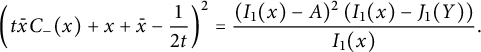 $$ \begin{align} \left( t \bar x C_-(x) +x+\bar x-\frac 1{2t} \right) ^{2} = \frac{ (I_1(x)- A)^2\left( {I_1(x)}- {J_1(Y)}\right) }{I_1(x)}. \end{align} $$
In the above expression, Y is the only root of
 $$ \begin{align} \Delta(y):=(1-ty)^2-4t^2\bar y(1+y)^2 \end{align} $$
that is a formal power series in t. Then,
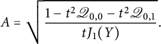 $$\begin{align*}A=\sqrt{\frac{1-t^2\mathscr Q_{0,0} -t^2\mathscr Q_{0,1}}{tJ_1(Y)}}. \end{align*}$$
The generating function $D(y)$
of walks ending on the diagonal satisfies
$D(y)$
of walks ending on the diagonal satisfies
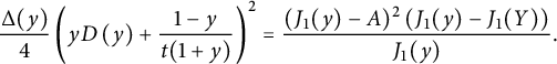 $$ \begin{align} \frac{\Delta(y) }4 \left( yD \left( y \right) + \frac {1-y}{t (1+y)} \right) ^{2} = \frac{ (J_1(y)- A)^2\left( J_1(y)- {J_1(Y)}\right) }{J_1(y)}. \end{align} $$
In particular, $C_-(x)$
,
$C_-(x)$
, $D(y)$
, and
$D(y)$
, and $C(x,y)$
are D-algebraic in all variables.
$C(x,y)$
are D-algebraic in all variables.
Our D-algebraicity result is not effective, and it seems hard to obtain an explicit differential equation in t for, say, the series $C(1,1)$
. This is already true in the quadrant case [Reference Bernardi, Bousquet-Mélou and Raschel2]. However, we indicate in Section 7.2 how one can write a differential equation in y for
$C(1,1)$
. This is already true in the quadrant case [Reference Bernardi, Bousquet-Mélou and Raschel2]. However, we indicate in Section 7.2 how one can write a differential equation in y for $D(y)$
.
$D(y)$
.
Proof The invariants of Proposition 3.3 are
 $$ \begin{align} I(x)= \left( 2\,tU \left( x,0 \right) +2\,x+2\bar x-\frac 1{t} \right) ^{2}, \qquad J(y)=\Delta(y) \left( yD \left( y\right) +{\frac {1-y}{t \left(1+ y \right) }} \right) ^{2}, \end{align} $$
where $\Delta (y)$
is defined by (7.3). We want to combine them polynomially with the invariants
$\Delta (y)$
is defined by (7.3). We want to combine them polynomially with the invariants $(I_1(x), J_1(y))$
given by (7.1) to form a pair of invariants
$(I_1(x), J_1(y))$
given by (7.1) to form a pair of invariants $(\tilde I(x), \tilde J(y))$
to which Lemma 2.6 would apply, thus proving that
$(\tilde I(x), \tilde J(y))$
to which Lemma 2.6 would apply, thus proving that $\tilde I(x)= \tilde J(y)$
is a series in t.
$\tilde I(x)= \tilde J(y)$
is a series in t.
Observe that $J(y) $
has a pole at
$J(y) $
has a pole at $y=0$
(coming from
$y=0$
(coming from $\Delta (y)$
) and at
$\Delta (y)$
) and at $y=-1$
. The modified invariant
$y=-1$
. The modified invariant $\tilde J(y)$
should have no poles. Observing that
$\tilde J(y)$
should have no poles. Observing that $J_1(0)=0$
, we first form the product
$J_1(0)=0$
, we first form the product $J(y) J_1(y)$
to remove the pole of
$J(y) J_1(y)$
to remove the pole of $J(y)$
at
$J(y)$
at $0$
. The resulting series now has a triple pole at
$0$
. The resulting series now has a triple pole at $-1$
, which can be removed by subtracting a cubic polynomial in
$-1$
, which can be removed by subtracting a cubic polynomial in $J_1(y)$
. This leads us to introduce
$J_1(y)$
. This leads us to introduce
 $$\begin{align*}\tilde J(y) = J(y) J_1(y)- 4J_1(y)^3 - A_2 J_1(y)^2 - A_1 J_1(y), \end{align*}$$
and to define accordingly
 $$\begin{align*}\tilde I(x) = I(x) I_1(x)- 4I_1(x)^3 - A_2 I_1(x)^2 - A_1 I_1(x), \end{align*}$$
for values of $A_2$
and
$A_2$
and $A_1$
that involve
$A_1$
that involve $D(-1), D'(-1)$
and various by-products of
$D(-1), D'(-1)$
and various by-products of $\mathscr Q(x,y)$
(we refer to our Maple session for details). Then, we use the functional equations satisfied by
$\mathscr Q(x,y)$
(we refer to our Maple session for details). Then, we use the functional equations satisfied by $U(x,y)$
,
$U(x,y)$
, $D(y)$
and
$D(y)$
and $\mathscr Q(x,y)$
to check that the ratio
$\mathscr Q(x,y)$
to check that the ratio
 $$\begin{align*}\frac{\tilde I(x) -\tilde J(y)}{\mathscr K(x,y)} \end{align*}$$
is a multiple of $xy$
, and conclude that
$xy$
, and conclude that $ \tilde I(x)= \tilde J(y)=A_0$
, for some series
$ \tilde I(x)= \tilde J(y)=A_0$
, for some series $A_0\in \mathbb {Q}((t))$
. Hence, denoting
$A_0\in \mathbb {Q}((t))$
. Hence, denoting $P(u)= 4u^3+A_2u^2+A_1u+A_0$
, we have
$P(u)= 4u^3+A_2u^2+A_1u+A_0$
, we have
 $$ \begin{align} I(x) I_1(x)= P(I_1(x)), \qquad \text{and} \qquad J(y) J_1(y)= P(J_1(y)). \end{align} $$
Since the left-hand sides of (7.2) and (7.4) in Theorem 7.1 are $I(x)/4$
and
$I(x)/4$
and $J(y)/4$
, the proof will be complete if we can prove that
$J(y)/4$
, the proof will be complete if we can prove that
 $$\begin{align*}P(u)= 4(u-A)^2(u-J_1(Y)). \end{align*}$$
We will identify the roots of $P(u)$
by looking at the values of y that cancel
$P(u)$
by looking at the values of y that cancel $J(y)$
, and thus
$J(y)$
, and thus $P(J_1(y))$
. First,
$P(J_1(y))$
. First, $\Delta (y)$
has a (unique) solution
$\Delta (y)$
has a (unique) solution $Y=\mathcal {O}(t^2)$
in
$Y=\mathcal {O}(t^2)$
in $\mathbb {Q}[[t]]$
. Thus,
$\mathbb {Q}[[t]]$
. Thus, $J_1(Y)=4t+\mathcal {O}(t^3)$
must be a root of P. Then, another root of
$J_1(Y)=4t+\mathcal {O}(t^3)$
must be a root of P. Then, another root of $J(y)$
arises from the factor of
$J(y)$
arises from the factor of $J(y)$
involving
$J(y)$
involving $D(y)$
. Indeed, the (unique) series
$D(y)$
. Indeed, the (unique) series $Y_0=1+2t+\mathcal {O}(t^2)$
such that
$Y_0=1+2t+\mathcal {O}(t^2)$
such that $Y_0=1+tY_0(1+Y_0)D(Y_0)$
is a double root of
$Y_0=1+tY_0(1+Y_0)D(Y_0)$
is a double root of $J(y)$
, and thus
$J(y)$
, and thus $J_1(Y_0)=1/(2t)+\mathcal {O}(1)$
is a double root of
$J_1(Y_0)=1/(2t)+\mathcal {O}(1)$
is a double root of $P(u)$
, unless
$P(u)$
, unless $J_1'(Y_0)=0$
, which we readily check not to be the case. At this stage, we can write
$J_1'(Y_0)=0$
, which we readily check not to be the case. At this stage, we can write
 $$\begin{align*}P(u)=4\left(u-J_1(Y_0)\right)^2\left(u-J_1(Y)\right). \end{align*}$$
However, we would like to make $A:=J_1(Y_0)$
more explicit. This can be done as follows: we return to the second identity of (7.6), replace
$A:=J_1(Y_0)$
more explicit. This can be done as follows: we return to the second identity of (7.6), replace $J(y)$
and
$J(y)$
and $J_1(y)$
by their expressions in terms of
$J_1(y)$
by their expressions in terms of $D(y)$
and
$D(y)$
and $\mathscr Q(0,y)$
, replace P by the above expression, and expand the result around
$\mathscr Q(0,y)$
, replace P by the above expression, and expand the result around $y=0$
. This gives
$y=0$
. This gives
 $$\begin{align*}tJ_1(Y) J_1(Y_0)^2= 1-t^2\mathscr Q_{0,0} -t^2\mathscr Q_{0,1} , \end{align*}$$
which concludes our derivation after choosing the correct (positive) sign for the square root.
The fact that all series under consideration are D-algebraic comes from the closure properties of D-algebraic series [Reference Bernardi, Bousquet-Mélou and Raschel2, Section 6.1], and from the fact that $\mathscr Q(x,y)$
is D-algebraic [Reference Bernardi, Bousquet-Mélou and Raschel2, Section 6.4].
$\mathscr Q(x,y)$
is D-algebraic [Reference Bernardi, Bousquet-Mélou and Raschel2, Section 6.4].
We can now specialize the first two equations of Theorem 7.1 to relate the series $C(1,1)$
to the quadrant series
$C(1,1)$
to the quadrant series $\mathscr Q$
.
$\mathscr Q$
.
Corollary 7.2 The generating function $C(1,1)$
counting walks with steps in
$C(1,1)$
counting walks with steps in $\{\rightarrow , \nearrow , \uparrow , \leftarrow , \downarrow \}$
that start from
$\{\rightarrow , \nearrow , \uparrow , \leftarrow , \downarrow \}$
that start from $(0,0)$
and avoid the negative quadrant is given by
$(0,0)$
and avoid the negative quadrant is given by
 $$ \begin{align} \frac 1 4 (1-5t)^2 \left( C(1,1)+\frac 1 t \right)^2 = \left( tC_-(1)+2 - \frac 1 {2t}\right)^2= \frac{(I_1(1)-A)^2(I_1(1)-J_1(Y))}{I_1(1)}, \end{align} $$
where $I_1(x)$
and
$I_1(x)$
and $J_1(y)$
are given by (7.1), and Y and A are defined in Theorem 7.1; in particular,
$J_1(y)$
are given by (7.1), and Y and A are defined in Theorem 7.1; in particular, $I_1(1)= 1+t\mathscr Q(1,0)$
.
$I_1(1)= 1+t\mathscr Q(1,0)$
.
7.2 An expression in terms of a weak invariant
Instead of using the quadrant-related invariants $I_1$
and
$I_1$
and $J_1$
of (7.1), one can use the analytic approach of [Reference Bernardi, Bousquet-Mélou and Raschel2, Section 5] and express
$J_1$
of (7.1), one can use the analytic approach of [Reference Bernardi, Bousquet-Mélou and Raschel2, Section 5] and express $D(y)$
(say) in terms of an explicit weak invariant
$D(y)$
(say) in terms of an explicit weak invariant $w(y)$
(expressed itself in terms of elliptic functions). Let us give a few details, using the notation of [Reference Bernardi, Bousquet-Mélou and Raschel2], which we will not redefine. First, the model denoted by
$w(y)$
(expressed itself in terms of elliptic functions). Let us give a few details, using the notation of [Reference Bernardi, Bousquet-Mélou and Raschel2], which we will not redefine. First, the model denoted by $\mathscr S$
here is model
$\mathscr S$
here is model $\#5$
in [Reference Bernardi, Bousquet-Mélou and Raschel2, Table 5]. Then, for t a small positive real number, the series
$\#5$
in [Reference Bernardi, Bousquet-Mélou and Raschel2, Table 5]. Then, for t a small positive real number, the series $D(y)$
can be defined analytically in the domain
$D(y)$
can be defined analytically in the domain $\mathcal G_{\mathcal L}$
, with finite limits on the boundary curve
$\mathcal G_{\mathcal L}$
, with finite limits on the boundary curve $\mathcal L$
[Reference Raschel and Trotignon31, Lemma 5]. This curve is bounded because
$\mathcal L$
[Reference Raschel and Trotignon31, Lemma 5]. This curve is bounded because $\mathscr S$
contains a West step [Reference Bernardi, Bousquet-Mélou and Raschel2, Lemma 5.2]. The points
$\mathscr S$
contains a West step [Reference Bernardi, Bousquet-Mélou and Raschel2, Lemma 5.2]. The points $0$
and
$0$
and $-1$
both belong to
$-1$
both belong to $\mathcal G_{\mathcal L}$
, by [Reference Bernardi, Bousquet-Mélou and Raschel2, Lemmas 5.2 and 5.8]. Hence, the invariant
$\mathcal G_{\mathcal L}$
, by [Reference Bernardi, Bousquet-Mélou and Raschel2, Lemmas 5.2 and 5.8]. Hence, the invariant $J(y)$
defined by (7.5), which is a simple variation on
$J(y)$
defined by (7.5), which is a simple variation on $D(y)$
, is meromorphic in
$D(y)$
, is meromorphic in $\mathcal G_{\mathcal L}$
, with finite limits on
$\mathcal G_{\mathcal L}$
, with finite limits on $\mathcal L$
, and exactly two poles in
$\mathcal L$
, and exactly two poles in $\mathcal G_{\mathcal L}$
, at
$\mathcal G_{\mathcal L}$
, at $0$
and
$0$
and $-1$
. The first pole is simple, and the second is double. Thus,
$-1$
. The first pole is simple, and the second is double. Thus, $J(y)$
is a weak invariant for the model
$J(y)$
is a weak invariant for the model $\mathscr S$
, in the sense of [Reference Bernardi, Bousquet-Mélou and Raschel2, Definition 5.4]. We can apply the (analytic) invariant lemma [Reference Bernardi, Bousquet-Mélou and Raschel2, Lemma 5.6]: there exists a polynomial
$\mathscr S$
, in the sense of [Reference Bernardi, Bousquet-Mélou and Raschel2, Definition 5.4]. We can apply the (analytic) invariant lemma [Reference Bernardi, Bousquet-Mélou and Raschel2, Lemma 5.6]: there exists a polynomial $P(u)$
(with complex coefficients that depend on the value t), of degree at most
$P(u)$
(with complex coefficients that depend on the value t), of degree at most $3$
, such that
$3$
, such that
 $$\begin{align*}J(y)= \Delta(y) \left( y D(y) + \frac{1-y}{t(1+y)}\right)^2 = \frac{P(w(y))}{(w(y)-w(0))(w(y)-w(-1))^2}. \end{align*}$$
As before, we can obtain some information on the roots of $P(u)$
by examining the roots of
$P(u)$
by examining the roots of $J(y)$
. First, the formal power series
$J(y)$
. First, the formal power series $Y=\mathcal {O}(t^2)$
that cancels
$Y=\mathcal {O}(t^2)$
that cancels $\Delta (y)$
specializes to the value denoted by
$\Delta (y)$
specializes to the value denoted by $y_2$
in [Reference Bernardi, Bousquet-Mélou and Raschel2, Lemma 5.1] (the value
$y_2$
in [Reference Bernardi, Bousquet-Mélou and Raschel2, Lemma 5.1] (the value $y_1$
is zero for this model). This is precisely the (unique) pole of
$y_1$
is zero for this model). This is precisely the (unique) pole of $w(y)$
in
$w(y)$
in $\mathcal G_{\mathcal L}$
, by [Reference Bernardi, Bousquet-Mélou and Raschel2, Proposition 5.5], and we conclude that
$\mathcal G_{\mathcal L}$
, by [Reference Bernardi, Bousquet-Mélou and Raschel2, Proposition 5.5], and we conclude that $P(u)$
has degree
$P(u)$
has degree $2$
at most. The series
$2$
at most. The series $Y_0=1+2t+\mathcal {O}(t ^3)$
that cancels the factor of
$Y_0=1+2t+\mathcal {O}(t ^3)$
that cancels the factor of $J(y)$
involving
$J(y)$
involving $D(y)$
can also be shown to specialize to a value
$D(y)$
can also be shown to specialize to a value $y_0$
of
$y_0$
of $\mathcal G_{\mathcal L}$
(because the positive point where the curve
$\mathcal G_{\mathcal L}$
(because the positive point where the curve $\mathcal L$
intersects the real axis, denoted by
$\mathcal L$
intersects the real axis, denoted by $Y(x_2)$
in [Reference Bernardi, Bousquet-Mélou and Raschel2], is
$Y(x_2)$
in [Reference Bernardi, Bousquet-Mélou and Raschel2], is $1/\sqrt t$
at first order, so that
$1/\sqrt t$
at first order, so that $y_0$
is smaller), so that
$y_0$
is smaller), so that $P(u)$
admits
$P(u)$
admits $w(y_0)$
as a double root. Finally,
$w(y_0)$
as a double root. Finally,
 $$ \begin{align} \qquad J(y)= \Delta(y) \left( y D(y) + \frac{1-y}{t(1+y)}\right)^2 = \frac{\alpha (w(y)-a)^2}{(w(y)-w(0))(w(y)-w(-1))^2} \hspace{-20pt}\end{align} $$
with $a=w(y_0)$
. One can determine
$a=w(y_0)$
. One can determine $\alpha $
and a in terms of
$\alpha $
and a in terms of $w(0)$
,
$w(0)$
, $w(-1)$
,
$w(-1)$
, $w'(0)$
, and
$w'(0)$
, and $w'(-1)$
by expanding this identity at first order around
$w'(-1)$
by expanding this identity at first order around $y=0$
and
$y=0$
and $y=-1$
.
$y=-1$
.
Alternatively, the above identity can be derived by combining the expression of $J(y)/4$
given in (7.4) in terms of
$J(y)/4$
given in (7.4) in terms of $J_1(y)$
(or equivalently, in terms of
$J_1(y)$
(or equivalently, in terms of $\mathscr Q(0,y)$
) with the following expression, borrowed from [Reference Bernardi, Bousquet-Mélou and Raschel2, Theorem 5.7]:
$\mathscr Q(0,y)$
) with the following expression, borrowed from [Reference Bernardi, Bousquet-Mélou and Raschel2, Theorem 5.7]:
 $$ \begin{align} \qquad y(1+t) \mathscr Q(0,y)=-y-\frac{1+t}{t(1+y)} -1 +\frac{1+t}t \left( \frac {w'(-1)}{w(y)-w(-1)} + \frac{w"(-1)}{2w'(-1)}\right). \hspace{-20pt}\end{align} $$
Indeed, the expression (7.1) of $J_1(y)$
then yields
$J_1(y)$
then yields
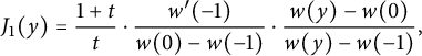 $$\begin{align*}J_1(y) =\frac{1+t} t \cdot \frac{w'(-1)}{w(0)-w(-1)} \cdot \frac{w(y)-w(0)}{w(y)-w(-1)}, \end{align*}$$
and, since $Y=y_2$
is a pole of
$Y=y_2$
is a pole of $w(y)$
,
$w(y)$
,
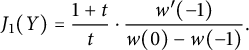 $$\begin{align*}J_1(Y)=\frac{1+t} t \cdot \frac{w'(-1)}{w(0)-w(-1)}. \end{align*}$$
We plug the latter two expressions in (7.4), and thus obtain the form (7.8), with values of a and $\alpha $
expressed in terms of
$\alpha $
expressed in terms of $w(0)$
,
$w(0)$
, $w(-1)$
,
$w(-1)$
, $w'(-1)$
, and A. Another by-product of this approach is an expression for the other series involved in the expression (7.4) of
$w'(-1)$
, and A. Another by-product of this approach is an expression for the other series involved in the expression (7.4) of $J(y)/4$
:
$J(y)/4$
:
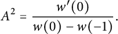 $$\begin{align*}A^2=\frac{w'(0)}{w(0)-w(-1)}. \end{align*}$$
Remarks
1. In [Reference Bernardi, Bousquet-Mélou and Raschel2, Section 6.5], we worked out an explicit differential equation in y for $\mathscr Q(0,y)$
, of order
$\mathscr Q(0,y)$
, of order $4$
, with polynomial coefficients in t and y, by combining the expression (7.9) and a first-order differential equation satisfied by
$4$
, with polynomial coefficients in t and y, by combining the expression (7.9) and a first-order differential equation satisfied by $w(y)$
. The same procedure could be applied to (7.8) to write down a differential equation, still of fourth order, for
$w(y)$
. The same procedure could be applied to (7.8) to write down a differential equation, still of fourth order, for $J(y)$
or
$J(y)$
or $D(y)$
.
$D(y)$
.
2. It is interesting to note that, while quadrant generating functions, when they can be expressed in terms of $w(y)$
, are in fact homographic functions of
$w(y)$
, are in fact homographic functions of $w(y)$
, the above expression of
$w(y)$
, the above expression of $J(y)$
has degree
$J(y)$
has degree $3$
in
$3$
in $w(y)$
. Moreover, the three-quadrant generating function
$w(y)$
. Moreover, the three-quadrant generating function $D(y)$
is no longer rational, but algebraic in
$D(y)$
is no longer rational, but algebraic in $w(y)$
. This is another sign of the higher difficulty of three-quadrant problems.
$w(y)$
. This is another sign of the higher difficulty of three-quadrant problems.
7.3 Harmonic functions
As already sketched in Remark 4.1 in the Kreweras case, we can relate the asymptotic behaviors of $\mathcal S$
-walks in
$\mathcal S$
-walks in $\mathcal {C}$
and
$\mathcal {C}$
and $\mathscr S$
-walks in
$\mathscr S$
-walks in $\mathcal {Q}$
, under highly plausible assumptions.
$\mathcal {Q}$
, under highly plausible assumptions.
Let us begin with quadrant $\mathscr S$
-walks. The number
$\mathscr S$
-walks. The number $\tilde q_{i,j}(n)$
of
$\tilde q_{i,j}(n)$
of $\mathscr S$
-walks of length n in the quadrant
$\mathscr S$
-walks of length n in the quadrant $\mathcal {Q}$
ending at
$\mathcal {Q}$
ending at $(i,j)$
is known to have the following asymptotic form [Reference Bostan, Raschel and Salvy6, Reference Denisov and Wachtel14]:
$(i,j)$
is known to have the following asymptotic form [Reference Bostan, Raschel and Salvy6, Reference Denisov and Wachtel14]:
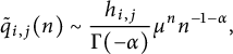 $$\begin{align*}\tilde q_{i,j}(n) \sim \frac{h_{i,j} }{\Gamma(-\alpha)} \mu^n n^{-1-\alpha}, \end{align*}$$
where $\mu \simeq 4.729$
is the positive solution of
$\mu \simeq 4.729$
is the positive solution of $\mu ^3+\mu ^2-18\mu -43=0$
, and
$\mu ^3+\mu ^2-18\mu -43=0$
, and $\alpha = \pi /\arccos (-c)\simeq 1.39$
, where
$\alpha = \pi /\arccos (-c)\simeq 1.39$
, where $c\simeq 0.626$
satisfies
$c\simeq 0.626$
satisfies $64\,{c}^{6}-64\,{c}^{4}+28\,{c}^{2}-5=0$
. The numbers
$64\,{c}^{6}-64\,{c}^{4}+28\,{c}^{2}-5=0$
. The numbers $h_{i,j}$
satisfy a
$h_{i,j}$
satisfy a $1/\mu $
-harmonic relation
$1/\mu $
-harmonic relation
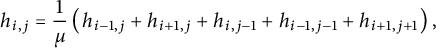 $$\begin{align*}h_{i,j}= \frac 1 \mu \left(h_{i-1,j}+h_{i+1,j}+h_{i,j-1}+h_{i-1,j-1}+h_{i+1,j+1} \right), \end{align*}$$
from which one derives the functional equation
 $$ \begin{align} \left(\!1+y+xy^2+x^2y+x^2y^2-\mu xy\!\right) \mathscr H(x,y)=\mathscr H(x,0) +(1+y) \mathscr H(0,y) -\mathscr H(0,0), \end{align} $$
where $ \mathscr H(x,y)=\sum _{i,j \ge 0} h_{i,j} x^i y^j$
. As discussed in [Reference Raschel30, Section 6], no simple expression is known for
$ \mathscr H(x,y)=\sum _{i,j \ge 0} h_{i,j} x^i y^j$
. As discussed in [Reference Raschel30, Section 6], no simple expression is known for $ \mathscr H(x,y)$
(the results of [Reference Raschel30] only hold for walks with no drift; the same is true for the results of [Reference Trotignon32] on harmonic functions in
$ \mathscr H(x,y)$
(the results of [Reference Raschel30] only hold for walks with no drift; the same is true for the results of [Reference Trotignon32] on harmonic functions in $\mathcal {C}$
).
$\mathcal {C}$
).
The number $ c_{i,j}(n)$
of
$ c_{i,j}(n)$
of $\mathcal S$
-walks of length n in the three-quadrant cone
$\mathcal S$
-walks of length n in the three-quadrant cone $\mathcal {C}$
ending at
$\mathcal {C}$
ending at $(i,j)$
is widely believed to have the following asymptotic form:
$(i,j)$
is widely believed to have the following asymptotic form:
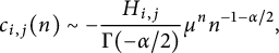 $$\begin{align*}c_{i,j}(n) \sim- \frac{H_{i,j} }{\Gamma(-\alpha/2)} \mu^n n^{-1-\alpha/2}, \end{align*}$$
with $\mu $
and
$\mu $
and $\alpha $
as above. More precisely, what is known is a pair of lower and upper bounds on
$\alpha $
as above. More precisely, what is known is a pair of lower and upper bounds on $c_{i,j}(n)$
that have the above form and differ simply by a multiplicative constant [Reference Mustapha28]. The minus sign has been chosen so that
$c_{i,j}(n)$
that have the above form and differ simply by a multiplicative constant [Reference Mustapha28]. The minus sign has been chosen so that $H_{i,j}>0$
.
$H_{i,j}>0$
.
If this holds, then
 $$\begin{align*}H_{i,j}=H_{j,i}= \frac 1 \mu \left(H_{i-1,j}+H_{i+1,j}+H_{i,j-1}+H_{i,j+1}+H_{i-1,j-1} \right), \end{align*}$$
which yields for the generating function $\mathcal H(x,y) = \sum _{j \ge 0, j\ge i} H_{i,j} x^{j-i} y^j$
the functional equation
$\mathcal H(x,y) = \sum _{j \ge 0, j\ge i} H_{i,j} x^{j-i} y^j$
the functional equation
 $$ \begin{align} \left(\!1+y+xy^2+x^2y+x^2y^2-\mu xy\!\right) \mathcal H(x,y)=\mathcal H_-(x)+\frac 1 2 \!\left(\! 2+2y+ xy^2-\mu xy\!\right) \!\mathcal H_d(y), \end{align} $$
where as before $\mathcal H_-(x)=\sum _{i>0} H_{-i,0} x^i$
and
$\mathcal H_-(x)=\sum _{i>0} H_{-i,0} x^i$
and $\mathcal H_d(y)=\mathcal H(0,y)$
.
$\mathcal H_d(y)=\mathcal H(0,y)$
.
We can now adapt the argument of Remark 4.1. The term $c(x,y)= \left ( 2+2y+ xy^2-\mu xy\right )/2$
satisfies
$c(x,y)= \left ( 2+2y+ xy^2-\mu xy\right )/2$
satisfies
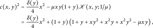 $$ \begin{align*} c(x,y)^2 &=\frac{\delta(y)}4 x^2 -\mu xy (1+y) \mathscr K(x,y;1/\mu) \\ & = \frac{\delta(y)}4 x^2+ (1+y) \left(1+y+xy^2+x^2y+x^2y^2-\mu xy\right), \end{align*} $$
where $\delta (y)= (\mu ^2y-2\mu y^2+y^3-4 y^2-8 y-4) y$
is the discriminant of
$\delta (y)= (\mu ^2y-2\mu y^2+y^3-4 y^2-8 y-4) y$
is the discriminant of $\mu xy \mathscr K(x,y;1/\mu ) $
with respect to x. Upon multiplying (7.11) by
$\mu xy \mathscr K(x,y;1/\mu ) $
with respect to x. Upon multiplying (7.11) by $\bar x^2(\mathcal H_-(x) - c(x,y) \mathcal H_d(y))$
, we conclude that the series
$\bar x^2(\mathcal H_-(x) - c(x,y) \mathcal H_d(y))$
, we conclude that the series
 $$\begin{align*}\overline{\mathscr H}(x,y) := \bar x^2\mathcal H \left( x,y \right) \left({ {\mathcal H_- \left( x \right)- c(x,y)\mathcal H_d \left( y \right) } } \right) + \bar x^2 { \left( 1+y \right) \mathcal H_d\left( y \right) ^{2}} \end{align*}$$
is a formal power series in x and y, which satisfies the same equation (7.10) as $\mathscr H(x,y)$
, as well as
$\mathscr H(x,y)$
, as well as
 $$\begin{align*}\overline{\mathscr H}(x,0)= \bar x^2 \mathcal H_-(x)^2, \qquad \text{and} \qquad \overline{\mathscr H}(0,y)= -\frac{\delta(y)}{4(1+y)}\mathcal H(0,y)^2 + \frac{H_{-1,0}^2}{1+y}. \end{align*}$$
In particular, $\overline {\mathscr H}(0,0)=H_{-1,0}^2$
. Let us now assume that:
$\overline {\mathscr H}(0,0)=H_{-1,0}^2$
. Let us now assume that:
-
•
$\mathscr H(x,y)$
is uniquely determined (up to a multiplicative factor) by equation (7.10) and the positivity of its coefficients; -
• the series
$\overline {\mathscr H}(x,y)$
has positive coefficients.


Then there exists a positive constant $\kappa ^2$
such that
$\kappa ^2$
such that $\overline {\mathscr H}(x,y)=\kappa ^2 \mathscr H(x,y)$
, which implies in particular that
$\overline {\mathscr H}(x,y)=\kappa ^2 \mathscr H(x,y)$
, which implies in particular that
 $$ \begin{align} \mathcal H_-(x) =\kappa x \sqrt{\mathscr H(x,0)} \qquad \text{and} \qquad \mathcal H_d(y) = 2\kappa \sqrt{-\frac{(1+y) \mathscr H(0,y)-\mathscr H(0,0)}{\delta(y)}}. \end{align} $$
Expanding these predictions at $x=0$
and
$x=0$
and $y=0$
gives
$y=0$
gives
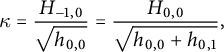 $$\begin{align*}\kappa = \frac{H_{-1,0}}{\sqrt{h_{0,0}}}= \frac{H_{0,0}}{\sqrt{h_{0,0}+h_{0,1}}}, \end{align*}$$
so that we expect
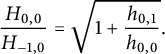 $$\begin{align*}\frac{H_{0,0}}{H_{-1,0}} = \sqrt{1 + \frac{h_{0,1}}{h_{0,0}}}. \end{align*}$$
This seems to hold, as shown by Figure 4, where we have plotted against $1/n$
the sequences
$1/n$
the sequences
 $$ \begin{align} \frac{c_{0,0}(n)}{c_{-1,0}(n)} \qquad \text{and} \qquad \sqrt{1 + \frac{\tilde q_{0,1}(n)}{\tilde q_{0,0}(n)}}. \end{align} $$
We have checked numerically more consequences of the prediction (7.12), like
 $$\begin{align*}\frac{H_{-1,0}}{H_{-2,0}}= 2\, \frac{h_{0,0}}{h_{1,0}} \qquad \text{and} \qquad \frac{H_{1,1}}{H_{0,0}}= \frac{\mu^2} 8 -1 +\frac 1 2 \cdot \frac{h_{0,1}+h_{0,2}}{h_{0,0}+h_{0,1}}, \end{align*}$$
each time with perfect agreement.
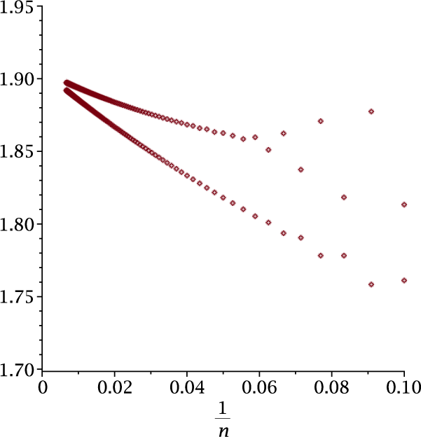
Figure 4: Plots of the sequences (7.13) against $1/n$
, for
$1/n$
, for $n\le 150$
.
$n\le 150$
.
8 The simple and diagonal models
In this section, we explain how the use of invariants also give new solutions of three-quadrant walks when $\mathcal S_1=\{\rightarrow , \uparrow , \leftarrow , \downarrow \}$
(simple model) and
$\mathcal S_1=\{\rightarrow , \uparrow , \leftarrow , \downarrow \}$
(simple model) and $\mathcal S_2=\{\nearrow , \nwarrow , \swarrow , \searrow \}$
(diagonal model). This may seem unexpected, for the following reason.
$\mathcal S_2=\{\nearrow , \nwarrow , \swarrow , \searrow \}$
(diagonal model). This may seem unexpected, for the following reason.
For both models, the basic functional equation of Lemma 2.1 holds (with a slightly different definition of U and D for the model $\mathcal S_2$
); but by Proposition 3.1, there is no way to decouple y in the desired form. Moreover, if we could still construct a pair of invariants involving
$\mathcal S_2$
); but by Proposition 3.1, there is no way to decouple y in the desired form. Moreover, if we could still construct a pair of invariants involving $U(x,0)$
, and relate it polynomially to the invariants
$U(x,0)$
, and relate it polynomially to the invariants $(I_1(x), J_1(y))$
that involve quadrant generating functions with steps in
$(I_1(x), J_1(y))$
that involve quadrant generating functions with steps in $\mathscr S_1$
or
$\mathscr S_1$
or $\mathscr S_2$
(the so-called Gessel model for
$\mathscr S_2$
(the so-called Gessel model for $\mathscr S_1$
, or its reflection in the main diagonal for
$\mathscr S_1$
, or its reflection in the main diagonal for $\mathscr S_2$
), then
$\mathscr S_2$
), then $U(x,0)$
would be algebraic, because quadrant walks with steps in
$U(x,0)$
would be algebraic, because quadrant walks with steps in $\mathscr S_1$
(or
$\mathscr S_1$
(or $\mathscr S_2$
) are algebraic. However, it is known that
$\mathscr S_2$
) are algebraic. However, it is known that $U(x,0)$
is transcendental for both models [Reference Bousquet-Mélou9].
$U(x,0)$
is transcendental for both models [Reference Bousquet-Mélou9].
However, for both models ( $\mathcal S=\mathcal S_1$
or
$\mathcal S=\mathcal S_1$
or $\mathcal S_2$
), it is natural [Reference Bousquet-Mélou9, Reference Bousquet-Mélou and Wallner12] to introduce the series
$\mathcal S_2$
), it is natural [Reference Bousquet-Mélou9, Reference Bousquet-Mélou and Wallner12] to introduce the series $A(x,y)$
defined by
$A(x,y)$
defined by
 $$ \begin{align} A(x,y)= C(x,y) - \frac 1 3 \left(Q(x,y) -\bar x^2 Q(\bar x,y) - \bar y^2 Q(x,\bar y) \right), \end{align} $$
where $Q(x,y)$
counts quadrant
$Q(x,y)$
counts quadrant $\mathcal S$
-walks. The series
$\mathcal S$
-walks. The series $A(x,y)$
is easily shown to satisfy the same functional equation (2.4) as
$A(x,y)$
is easily shown to satisfy the same functional equation (2.4) as $C(x,y)$
, but with the initial term
$C(x,y)$
, but with the initial term $1$
replaced by
$1$
replaced by $ (2+\bar x^2+\bar y^2)/3$
. And then the heart of [Reference Bousquet-Mélou9] is to prove that
$ (2+\bar x^2+\bar y^2)/3$
. And then the heart of [Reference Bousquet-Mélou9] is to prove that $A(x,y)$
is algebraic, for both models.
$A(x,y)$
is algebraic, for both models.
Hence, a natural idea is to try to apply the tools developed in this paper to $A(x,y)$
rather than
$A(x,y)$
rather than $C(x,y)$
. We shall see that the new series
$C(x,y)$
. We shall see that the new series $U(x,y)$
, defined from
$U(x,y)$
, defined from $A(x,y)$
rather than
$A(x,y)$
rather than $C(x,y)$
, satisfies an equation similar to the one of Lemma 2.1, but with an initial term
$C(x,y)$
, satisfies an equation similar to the one of Lemma 2.1, but with an initial term $y(1+x^e)$
instead of y (the exponent e is
$y(1+x^e)$
instead of y (the exponent e is $2$
for the simple model, and
$2$
for the simple model, and $1$
for the diagonal model). And now this term decouples, whereas y does not. This yields new
$1$
for the diagonal model). And now this term decouples, whereas y does not. This yields new $\mathscr S$
-invariants, involving
$\mathscr S$
-invariants, involving $A(x,y)$
, and ultimately a relation between
$A(x,y)$
, and ultimately a relation between $A(x,y)$
and the generating function of quadrant walks with Gessel’s steps.
$A(x,y)$
and the generating function of quadrant walks with Gessel’s steps.
We finally derive from this the harmonic functions $H_{i,j}$
for the simple and diagonal models in the three-quadrant plane. The generating functions
$H_{i,j}$
for the simple and diagonal models in the three-quadrant plane. The generating functions $\sum _{(i,j)\in \mathcal C} H_{i,j} x^i y^j$
are algebraic in both cases, even though the generating functions
$\sum _{(i,j)\in \mathcal C} H_{i,j} x^i y^j$
are algebraic in both cases, even though the generating functions $C(x,y)$
are D-finite but transcendental. We do not work out more exact results (for instance, the degree of
$C(x,y)$
are D-finite but transcendental. We do not work out more exact results (for instance, the degree of $A(x,y)$
or of the series
$A(x,y)$
or of the series $A_{i,j}$
), as such results already appear in [Reference Bousquet-Mélou9].
$A_{i,j}$
), as such results already appear in [Reference Bousquet-Mélou9].
8.1 The simple model
When $\mathcal S=\{\rightarrow , \uparrow , \leftarrow , \downarrow \}$
, the series
$\mathcal S=\{\rightarrow , \uparrow , \leftarrow , \downarrow \}$
, the series $A(x,y)$
defined by (8.1) satisfies
$A(x,y)$
defined by (8.1) satisfies
 $$ \begin{align} \qquad (1-t(x+\bar x+y+\bar y))A(x,y)= (2+\bar x^2+\bar y^2)/3-t\bar y A_-(\bar x) -t \bar x A_-(\bar y) , \hspace{-20pt}\end{align} $$
where the series $A_-(\bar x)$
is defined in a similar fashion as
$A_-(\bar x)$
is defined in a similar fashion as $C_-(\bar x)$
(see (2.3)). The series
$C_-(\bar x)$
(see (2.3)). The series $A(x,y)$
has a simple combinatorial interpretation: it counts weighted walks in the three-quadrant cone
$A(x,y)$
has a simple combinatorial interpretation: it counts weighted walks in the three-quadrant cone $\mathcal {C}$
, starting either from
$\mathcal {C}$
, starting either from $(0,0)$
, or from
$(0,0)$
, or from $(-2,0)$
, or from
$(-2,0)$
, or from $(0,-2)$
, with a weight
$(0,-2)$
, with a weight $2/3$
in the first case, and
$2/3$
in the first case, and $1/3$
in the other two. We now define two series
$1/3$
in the other two. We now define two series $U(x,y)$
and
$U(x,y)$
and $D(y)$
by
$D(y)$
by
 $$ \begin{align} A(x,y) = \bar x U(\bar x,xy)+ D(xy)+ \bar y U(\bar y,xy). \end{align} $$
Note that they do not have the same combinatorial meaning as in the previously solved four models. We can reproduce the step-by-step arguments that led to Lemma 2.1, and we thus obtain
 $$ \begin{align} \qquad 2 xy\mathscr K(x,y)U(x,y)= \frac 2 3 y(1+x^2) +y\left(2tx(1+y)-1\right)D(y)-2 tU(x, 0), \hspace{-20pt}\end{align} $$
where $\mathscr K(x,y)=1-t\mathscr S(x,y)=1-t(x+\bar x +xy+\bar x\bar y)$
is the step polynomial of Gessel’s model. Compared with the original functional equation (2.12), the only thing that has changed is the initial term y, which has become
$\mathscr K(x,y)=1-t\mathscr S(x,y)=1-t(x+\bar x +xy+\bar x\bar y)$
is the step polynomial of Gessel’s model. Compared with the original functional equation (2.12), the only thing that has changed is the initial term y, which has become $2 y(1+x^2) /3$
.
$2 y(1+x^2) /3$
.
For the model $\mathscr S$
, we know two pairs of invariants (see Table 3): one is rational, and will not be used; the other takes the form (2.24) and involves quadrant generating functions:
$\mathscr S$
, we know two pairs of invariants (see Table 3): one is rational, and will not be used; the other takes the form (2.24) and involves quadrant generating functions:
 $$ \begin{align} \qquad I_1(x)= t\mathscr Q(x, 0)+ \bar x , \qquad J_1(y) =-t(1+y)\mathscr Q(0, y)+t\mathscr Q_{0, 0} +\frac y{t(1+y)}. \hspace{-20pt}\end{align} $$
These two series are algebraic, and we refer to [Reference Bostan and Kauers5, Reference Bousquet-Mélou8] for explicit expressions. They satisfy
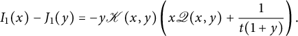 $$\begin{align*}I_1(x)-J_1(y)= -y\mathscr K(x,y) \left(x \mathscr Q(x,y) + \frac 1 {t(1+y)}\right). \end{align*}$$
We will obtain expressions for $U(x,0)$
and
$U(x,0)$
and $D(y)$
in terms of
$D(y)$
in terms of $I_1(x)$
and
$I_1(x)$
and $J_1(y)$
, which are reminiscent of those of the previous section (Theorem 7.1). Given that a polynomial identity relates
$J_1(y)$
, which are reminiscent of those of the previous section (Theorem 7.1). Given that a polynomial identity relates $(I_0(x),J_0(y))$
and
$(I_0(x),J_0(y))$
and $(I_1(x),J_1(y))$
, of degree
$(I_1(x),J_1(y))$
, of degree $3$
in the latter pair, we could also decrease to
$3$
in the latter pair, we could also decrease to $2$
the degree in
$2$
the degree in $I_1(x)$
and
$I_1(x)$
and $J_1(y)$
of our expressions, upon introducing
$J_1(y)$
of our expressions, upon introducing $I_0(x)$
and
$I_0(x)$
and $J_0(y)$
.
$J_0(y)$
.
Theorem 8.1 Let $I_1(x)$
and
$I_1(x)$
and $J_1(y)$
be defined as above. The generating function
$J_1(y)$
be defined as above. The generating function $A(x,y)$
defined by (8.1) satisfies equation (8.2), where
$A(x,y)$
defined by (8.1) satisfies equation (8.2), where $A_-(x)$
can be expressed in terms of
$A_-(x)$
can be expressed in terms of $I_1$
and
$I_1$
and $J_1$
by
$J_1$
by
 $$ \begin{align} \left(3 t \bar x A_-(x) +1+\bar x^2-\frac{\bar x}{t} \right) ^{2} = I_1(x)\, \big(I_1(x)- B\big)^2\big(I_1(x)- J_1(Y)\big). \end{align} $$
In the above expression, Y is the only root of
 $$ \begin{align} \Delta(y)= 1-4t^2\bar y (1+y)^2 \end{align} $$
that is a formal power series in t, and
 $$\begin{align*}B=\frac 1 t + 2 t \mathscr Q_{0,0} - \frac{J_1(Y)}2. \end{align*}$$
The generating function $D(y)$
defined by (8.3) satisfies
$D(y)$
defined by (8.3) satisfies
 $$ \begin{align} \qquad \frac 94 {\Delta(y) } \left( yD ( y) +\frac {2y}{3t^2(1+y)^2} \right) ^{2} = J_1(y)\, \big(J_1(y)- B\big)^2\big(J_1(y)- J_1(Y)\big). \hspace{-20pt}\end{align} $$
In particular, the series $A_-(x)$
,
$A_-(x)$
, $D(y)$
, and
$D(y)$
, and $A(x,y)$
are algebraic.
$A(x,y)$
are algebraic.
Remark 8.2
Degrees and rational parametrizations of $A_-(x)$
and
$A_-(x)$
and $D(y)$
. In [Reference Bousquet-Mélou8], the series
$D(y)$
. In [Reference Bousquet-Mélou8], the series $\mathscr Q(xt,0)$
and
$\mathscr Q(xt,0)$
and $\mathscr Q(0,y)$
(involved in the expressions of
$\mathscr Q(0,y)$
(involved in the expressions of $I_1(xt)$
and
$I_1(xt)$
and $J_1(y)$
, respectively) are expressed as rational functions in four algebraic series denoted by T,
$J_1(y)$
, respectively) are expressed as rational functions in four algebraic series denoted by T, $Z=\sqrt T$
,
$Z=\sqrt T$
, $U\equiv U(x)$
, and
$U\equiv U(x)$
, and $V\equiv V(y)$
. Here, T has degree
$V\equiv V(y)$
. Here, T has degree $4$
over
$4$
over $\mathbb {Q}(t)$
, whereas
$\mathbb {Q}(t)$
, whereas $U(x)$
is cubic over
$U(x)$
is cubic over $\mathbb {Q}(x, T)$
and
$\mathbb {Q}(x, T)$
and $V(y)$
is cubic over
$V(y)$
is cubic over $\mathbb {Q}(y,T)$
. All these series are series in
$\mathbb {Q}(y,T)$
. All these series are series in $t^2$
. Moreover,
$t^2$
. Moreover, $t^2\in \mathbb {Q}(T)$
,
$t^2\in \mathbb {Q}(T)$
, $x\in \mathbb {Q}(T,U)$
, and
$x\in \mathbb {Q}(T,U)$
, and $y\in \mathbb {Q}(T,V)$
. One can derive from these results rational expressions of
$y\in \mathbb {Q}(T,V)$
. One can derive from these results rational expressions of $I_1(xt)/t$
and
$I_1(xt)/t$
and $J_1(y)/t$
in terms of
$J_1(y)/t$
in terms of $\sqrt T$
, U, and V, and well as the following simple expressions:
$\sqrt T$
, U, and V, and well as the following simple expressions:
 $$\begin{align*}J_1(Y)=\frac{256 t T \sqrt{T} }{(T+3)^3}, \qquad B= {\frac {64t\,T\sqrt{T} \left( {T}^{2}+4\,T-1 \right) }{ \left( T-1 \right) \left( T+3 \right) ^{3}}}. \end{align*}$$
Details of these calculations are given in our Maple session. Using (8.6) (resp. (8.8)), we then obtain a rational expression of
 $$\begin{align*}\left( 3 \bar x A_-(xt) +1 + \frac{\bar x^2}{t^2}-\frac{\bar x}{t^2}\right)^2 \qquad \qquad \left( \text{resp.} \quad \left( y D(y) + \frac{2y}{3t^2(1+y)^2} \right)^2\right) \end{align*}$$
in terms of T and U (resp. T and V), showing that this series has degree $12$
only (as
$12$
only (as $\sqrt T$
is not involved here). Moreover, this rational expression is of the form
$\sqrt T$
is not involved here). Moreover, this rational expression is of the form $T \operatorname {\mathrm {Rat}}(T,U)^2$
(resp.
$T \operatorname {\mathrm {Rat}}(T,U)^2$
(resp. $T \operatorname {\mathrm {Rat}}(T,V)^2$
) for some rational function
$T \operatorname {\mathrm {Rat}}(T,V)^2$
) for some rational function $\operatorname {\mathrm {Rat}}$
, so that
$\operatorname {\mathrm {Rat}}$
, so that
 $$\begin{align*}3 \bar x A_-(xt) +1 + \frac{\bar x^2}{t^2}-\frac{\bar x}{t^2} \qquad \qquad \left( \text{resp.} \quad y D(y) + \frac{2y}{3t^2(1+y)^2} \right) \end{align*}$$
belongs to $\sqrt T \mathbb {Q}(T,U)$
(resp.
$\sqrt T \mathbb {Q}(T,U)$
(resp. $\sqrt T \mathbb {Q}(T,V)$
), and hence to the same extension of degree
$\sqrt T \mathbb {Q}(T,V)$
), and hence to the same extension of degree $24$
of
$24$
of $\mathbb {Q}(t,x)$
(resp.
$\mathbb {Q}(t,x)$
(resp. $\mathbb {Q}(t,y)$
) as
$\mathbb {Q}(t,y)$
) as $\mathscr Q(xt,0)$
(resp.
$\mathscr Q(xt,0)$
(resp. $\mathscr Q(0,y)$
). This is in contrast with the Kreweras-like models solved in Sections 4–6, for which the degree of
$\mathscr Q(0,y)$
). This is in contrast with the Kreweras-like models solved in Sections 4–6, for which the degree of $C_-(x)$
and
$C_-(x)$
and $D(y)$
is twice the degree of
$D(y)$
is twice the degree of $\mathscr Q(x,0)$
(or
$\mathscr Q(x,0)$
(or $\mathscr Q(0,y)$
).
$\mathscr Q(0,y)$
).
Proof of Theorem 8.1
We start from the functional equation (8.4), and observe that we have a decoupling relation:
 $$\begin{align*}y (1+x^2) = (2tx(1+y)-1)G(y)+F(x) + H(x,y) \mathscr K(x,y), \end{align*}$$
where
 $$\begin{align*}F(x)=-1-\bar x^2+ \frac 1{tx}, \quad G(y)= \frac{y}{t^2(1+y)^2}, \quad H(x,y)=\frac {y\left(1-t(x+\bar x+\bar x y+xy)\right)}{t^2(1+y)^2}. \end{align*}$$
This, together with Lemma 2.3, leads us to define a new pair of $\mathscr S$
-invariants
$\mathscr S$
-invariants $(I(x),J(y))$
:
$(I(x),J(y))$
:
 $$\begin{align*}I(x)= \left(2tU(x,0) + \frac 2 3 \left( 1+\bar x^2- \frac{\bar x}{t}\right)\right)^2, \qquad J(y)= \Delta(y) \left(yD(y) + \frac{2y}{3t^2(1+y)^2}\right)^2, \end{align*}$$
where $\Delta (y)$
is given by (8.7). We want to combine this new pair with the pair
$\Delta (y)$
is given by (8.7). We want to combine this new pair with the pair $(I_1(x), J_1(y))$
given by (8.5) to form a pair of invariants
$(I_1(x), J_1(y))$
given by (8.5) to form a pair of invariants $(\tilde I(x), \tilde J(y))$
to which Lemma 2.6 would apply, thus proving that
$(\tilde I(x), \tilde J(y))$
to which Lemma 2.6 would apply, thus proving that $\tilde I(x)= \tilde J(y)$
is a series in t.
$\tilde I(x)= \tilde J(y)$
is a series in t.
Observe that $I_1(x)$
and
$I_1(x)$
and $I(x)$
have poles at
$I(x)$
have poles at $x=0$
, whereas
$x=0$
, whereas $J_1(y)$
and
$J_1(y)$
and $J(y) $
have poles at
$J(y) $
have poles at $y=-1$
(only). More precisely, the series
$y=-1$
(only). More precisely, the series $I(x)$
has a (quadruple) pole at
$I(x)$
has a (quadruple) pole at $0$
, which can be removed by subtracting a well-chosen quartic polynomial in
$0$
, which can be removed by subtracting a well-chosen quartic polynomial in $I_1(x)$
. This leads us to introduce
$I_1(x)$
. This leads us to introduce
 $$\begin{align*}\tilde I(x) = I(x) - \frac 4 9 I_1(x)^4-B_3 I_1(x)^3 - B_2 I_1(x)^2 - B_1 I_1(x), \end{align*}$$
and analogously
 $$\begin{align*}\tilde J(y) = J(y) - \frac 4 9 J_1(y)^4 - B_3 J_1(y)^3 - B_2 J_1(y)^2 - B_1 J_1(y), \end{align*}$$
for values of $B_3$
,
$B_3$
, $B_2$
, and
$B_2$
, and $B_1$
that involve
$B_1$
that involve $U_{0,0}, U_{1,0}$
and various by-products of
$U_{0,0}, U_{1,0}$
and various by-products of $\mathscr Q(x,y)$
(we refer to our Maple session for details; we have denoted the auxiliary series
$\mathscr Q(x,y)$
(we refer to our Maple session for details; we have denoted the auxiliary series $B_i$
instead of
$B_i$
instead of $A_i$
to avoid any confusion with the series
$A_i$
to avoid any confusion with the series $A(x,y)$
or
$A(x,y)$
or $A_-(x)$
). Then, we use the functional equations satisfied by
$A_-(x)$
). Then, we use the functional equations satisfied by $U(x,y)$
,
$U(x,y)$
, $D(y)$
, and
$D(y)$
, and $\mathscr Q(x,y)$
to check that the ratio
$\mathscr Q(x,y)$
to check that the ratio
 $$\begin{align*}\frac{\tilde I(x) -\tilde J(y)}{\mathscr K(x,y)} \end{align*}$$
is a multiple of $xy$
, and conclude that
$xy$
, and conclude that $ \tilde I(x)= \tilde J(y)=B_0$
, for some series
$ \tilde I(x)= \tilde J(y)=B_0$
, for some series $B_0\in \mathbb {Q}((t))$
. By expanding
$B_0\in \mathbb {Q}((t))$
. By expanding $\tilde J(y)$
at
$\tilde J(y)$
at $y=0$
, we realize that
$y=0$
, we realize that $B_0=0$
. Hence, denoting by
$B_0=0$
. Hence, denoting by $P(u)= 4u^3/9+B_3u^2+B_2u+B_1$
, we have
$P(u)= 4u^3/9+B_3u^2+B_2u+B_1$
, we have
 $$ \begin{align} I(x)= I_1(x)P(I_1(x)) \qquad \text{and} \qquad J(y)= J_1(y)P(J_1(y)). \end{align} $$
We can express the roots of P in terms of the series $\mathscr Q$
by looking at the formal power series
$\mathscr Q$
by looking at the formal power series $X\in \mathbb {Q}[[t]]$
or
$X\in \mathbb {Q}[[t]]$
or $Y\in \mathbb {Q}[[t]]$
that cancel
$Y\in \mathbb {Q}[[t]]$
that cancel $I(x)$
or
$I(x)$
or $J(y)$
. First,
$J(y)$
. First, $\Delta (y)$
has a unique solution in
$\Delta (y)$
has a unique solution in $\mathbb {Q}[[t]]$
, which we denote by
$\mathbb {Q}[[t]]$
, which we denote by $Y=4t^2+\mathcal {O}(t^4)$
. Thus,
$Y=4t^2+\mathcal {O}(t^4)$
. Thus, $J_1(Y)=4t+\mathcal {O}(t^3)$
must be a root of P. Then, another root of P arises from the series
$J_1(Y)=4t+\mathcal {O}(t^3)$
must be a root of P. Then, another root of P arises from the series $X=t+\mathcal {O}(t^3)$
such that
$X=t+\mathcal {O}(t^3)$
such that $I(X)=0$
, that is,
$I(X)=0$
, that is, $X=3t^2U(X, 0)X^2+tX^2+t$
. This series is a double root of
$X=3t^2U(X, 0)X^2+tX^2+t$
. This series is a double root of $I(x)$
, and thus
$I(x)$
, and thus $I_1(X)=1/t+\mathcal {O}(t^3)$
is a double root of
$I_1(X)=1/t+\mathcal {O}(t^3)$
is a double root of $P(u)$
, unless
$P(u)$
, unless $I_1'(X)=0$
, which we readily check not to be the case. At this stage, we can write
$I_1'(X)=0$
, which we readily check not to be the case. At this stage, we can write
 $$\begin{align*}P(u)=\frac 4 9 \big(u-J_1(Y)\big)\big(u-I_1(X)\big)^2, \end{align*}$$
but we still have to relate the double root $B:=I_1(X)$
to
$B:=I_1(X)$
to $\mathscr Q$
. We expand around
$\mathscr Q$
. We expand around $x=0$
the first identity of (8.9), and obtain the expression of the root B given in the statement of the theorem.
$x=0$
the first identity of (8.9), and obtain the expression of the root B given in the statement of the theorem.
The expressions (8.6) and (8.8), which are those of $9I(x)/4$
and
$9I(x)/4$
and $9J(y)/4$
, are now proved.
$9J(y)/4$
, are now proved.
Here is now our description of the harmonic function associated with simple walks in $\mathcal {C}$
.
$\mathcal {C}$
.
Corollary 8.3 For $(i,j) \in \mathcal C$
, there exists a positive constant
$(i,j) \in \mathcal C$
, there exists a positive constant $H_{i,j}$
such that, as
$H_{i,j}$
such that, as $n\rightarrow \infty $
with
$n\rightarrow \infty $
with $n\equiv i+j\ \mod 2$
,
$n\equiv i+j\ \mod 2$
,
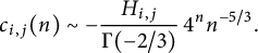 $$ \begin{align} c_{i,j}(n) \sim -\frac{H_{i,j}}{\Gamma(-2/3)}\, 4^n n^{-5/3}. \end{align} $$
The generating function
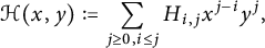 $$\begin{align*}\mathcal H(x,y):=\sum_{j\ge 0, i\le j} H_{i,j} x^{j-i} y^j, \end{align*}$$
which is a formal power series in x and y, is algebraic of degree $9$
, given by
$9$
, given by
 $$\begin{align*}\left(1+y+x^2y+x^2y^2-4xy\right) \mathcal H(x,y)= \mathcal H_-(x)+(1+y-2xy) \mathcal H_d(y), \end{align*}$$
where
 $$\begin{align*}\mathcal H_-(x):=\sum_{i>0} H_{-i,0} x^i\qquad \text{and} \qquad \mathcal H_d(y):=\sum_{i\ge 0} H_{i,i}y^i. \end{align*}$$
Each of these series is algebraic of degree $3$
. Let us define
$3$
. Let us define $L\equiv L(x)=\sqrt 3+\mathcal {O}(x)$
and
$L\equiv L(x)=\sqrt 3+\mathcal {O}(x)$
and $P\equiv P(y)=1/3+\mathcal {O}(y)$
by
$P\equiv P(y)=1/3+\mathcal {O}(y)$
by
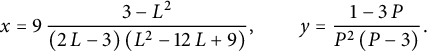 $$\begin{align*}x=9\,{\frac {3-{L}^{2}}{ \left( 2\,L-3 \right) \left( {L}^{2}-12\,L+9 \right) }}, \qquad y={\frac {1-3\,P}{{P}^{2} \left( P-3 \right) }}. \end{align*}$$
Then
 $$ \begin{align} \mathcal H_-(x) = {\frac {128\,\sqrt {3} x \left( 2\,L-3 \right) }{9\, \left( L-3 \right) ^{2}}} \qquad \text{and} \qquad \mathcal H_d(y) = {\frac {64\,\sqrt {3} \left( P+1 \right) \left( P-3 \right) ^{2}{P}^ {3}}{27\, \left(1- P \right) ^{5}}}. \end{align} $$
Note that an explicit expression of $\mathcal H_d(y)$
was given in [Reference Trotignon32, equation (53)] in terms of radicals. The fact that the degree is only
$\mathcal H_d(y)$
was given in [Reference Trotignon32, equation (53)] in terms of radicals. The fact that the degree is only $3$
is not obvious on this alternative expression.
$3$
is not obvious on this alternative expression.
Proof (sketched)
The principle is the same as in the proof of Corollary 1.4, where we determined a harmonic function for (reverse) Kreweras’ walks in three quadrants. We focus on the asymptotic behavior of the coefficients $a_{i,j}(n)$
of the series
$a_{i,j}(n)$
of the series $A(x,y)$
defined by (8.1), and establish for them the estimate (8.10): since the coefficients of
$A(x,y)$
defined by (8.1), and establish for them the estimate (8.10): since the coefficients of $Q(x,y)$
grow like
$Q(x,y)$
grow like $4^n n^{-3}$
only, the coefficients
$4^n n^{-3}$
only, the coefficients $a_{i,j}(n)$
and
$a_{i,j}(n)$
and $c_{i,j}(n)$
are asymptotically equivalent.
$c_{i,j}(n)$
are asymptotically equivalent.
We start from the expressions of $A_-(x)$
and
$A_-(x)$
and $D(y)$
given in Theorem 8.1, and use the results of [Reference Bousquet-Mélou8] to express
$D(y)$
given in Theorem 8.1, and use the results of [Reference Bousquet-Mélou8] to express $A_-(xt)$
and
$A_-(xt)$
and $D(y)$
rationally in terms of three algebraic series denoted by
$D(y)$
rationally in terms of three algebraic series denoted by $\sqrt T$
,
$\sqrt T$
, $U(x)$
, and
$U(x)$
, and $V(y)$
, as described in Remark 8.2.
$V(y)$
, as described in Remark 8.2.
We then perform the singular analysis of T, $U(x)$
, and
$U(x)$
, and $V(y)$
in the neighborhood of their dominant singularity, located at
$V(y)$
in the neighborhood of their dominant singularity, located at $t^2=1/16$
. The series
$t^2=1/16$
. The series $L(x)$
(resp.
$L(x)$
(resp. $P(y)$
) occurs in the singular expansion of
$P(y)$
) occurs in the singular expansion of $U(x)$
(resp.
$U(x)$
(resp. $V(y)$
). The three series T,
$V(y)$
). The three series T, $U(x)$
, and
$U(x)$
, and $V(y)$
have a singular behavior in
$V(y)$
have a singular behavior in $(1-16t^2)^{1/3}$
, but we need to work out more terms because cancellations occur when moving from these series to
$(1-16t^2)^{1/3}$
, but we need to work out more terms because cancellations occur when moving from these series to $A_-(xt)$
and
$A_-(xt)$
and $D(y)$
, which are found to have a singular behavior in
$D(y)$
, which are found to have a singular behavior in $(1-16t^2)^{2/3}$
. This is how we finally obtain the expressions of
$(1-16t^2)^{2/3}$
. This is how we finally obtain the expressions of $\mathcal H_-(x)$
and
$\mathcal H_-(x)$
and $\mathcal H_d(y)$
. The expression of
$\mathcal H_d(y)$
. The expression of $\mathcal H(x,y)$
simply comes from the harmonicity of
$\mathcal H(x,y)$
simply comes from the harmonicity of $H_{i,j}$
.
$H_{i,j}$
.
Remark 8.4 In passing, we have also determined the harmonic function for Gessel’s walks in the first quadrant: for $(i,j)\in \mathcal {Q}$
and
$(i,j)\in \mathcal {Q}$
and $n\equiv i$
mod
$n\equiv i$
mod $2$
, the number of n-step walks ending at
$2$
, the number of n-step walks ending at $(i,j)$
is asymptotic to
$(i,j)$
is asymptotic to
 $$\begin{align*}\frac{h_{i,j}}{\Gamma(-4/3)} 4^n n^{-7/3}, \end{align*}$$
where
 $$\begin{align*}\sum_{i\ge0} h_{i,0} x^i=48 \sqrt {3} \ \frac {\left( 2\,L-3 \right) ^{2}}{ \left( L-3 \right) ^{4}} \qquad\text{and} \qquad \sum_{j\ge 0} h_{0,j} y^i=\frac{32}{\sqrt 3}{\frac {{P}^{3} \left(3- P \right) }{ \left( P+1 \right) \left( P-1 \right) ^{4}}}. \end{align*}$$
We observe that these two series are cubic over $\mathbb {Q}(\sqrt 3)$
, as the two univariate series describing the harmonic function of simple walks in three quadrants (see (8.11)). This is in contrast with the previously solved models, where the degree of
$\mathbb {Q}(\sqrt 3)$
, as the two univariate series describing the harmonic function of simple walks in three quadrants (see (8.11)). This is in contrast with the previously solved models, where the degree of $\mathcal H_-(x)$
and
$\mathcal H_-(x)$
and $\mathcal H_d(y)$
is twice the degree of the corresponding quadrant harmonic function (see, for instance, (1.11) and (1.14)). As already mentioned in Remark 8.2, a similar property holds at the level of (counting) generating functions:
$\mathcal H_d(y)$
is twice the degree of the corresponding quadrant harmonic function (see, for instance, (1.11) and (1.14)). As already mentioned in Remark 8.2, a similar property holds at the level of (counting) generating functions: $\mathscr Q(x,0)$
and
$\mathscr Q(x,0)$
and $\mathscr Q(0,y)$
have degree
$\mathscr Q(0,y)$
have degree $24$
, and the same holds for
$24$
, and the same holds for $A_-(x)$
and
$A_-(x)$
and $D(y)$
.
$D(y)$
.
8.2 The diagonal model
When $\mathcal S=\{\nearrow , \nwarrow , \swarrow , \searrow \}$
, the series
$\mathcal S=\{\nearrow , \nwarrow , \swarrow , \searrow \}$
, the series $A(x,y)$
defined by (8.1) satisfies
$A(x,y)$
defined by (8.1) satisfies
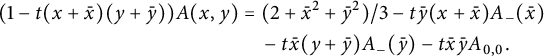 $$ \begin{align} (1-t(x+\bar x)(y+\bar y))A(x,y)&= (2+\bar x^2+\bar y^2)/3-t\bar y (x+\bar x)A_-(\bar x)\nonumber \\ &\quad -t \bar x(y+\bar y) A_-(\bar y)-t\bar x\bar y A_{0,0}. \end{align} $$
As before, this series counts weighted walks in the three-quadrant cone starting either from $(0,0)$
, or from
$(0,0)$
, or from $(-2,0)$
, or from
$(-2,0)$
, or from $(0,-2)$
, with a weight
$(0,-2)$
, with a weight $2/3$
in the first case, and
$2/3$
in the first case, and $1/3$
in the other two. As discussed in Lemma 2.1 for the corresponding series
$1/3$
in the other two. As discussed in Lemma 2.1 for the corresponding series $C(x,y)$
, it makes sense to define two series
$C(x,y)$
, it makes sense to define two series $U(x,y)$
and
$U(x,y)$
and $D(y)$
by
$D(y)$
by
 $$ \begin{align} A(x,y) = \bar x^2 U(\bar x^2,xy)+ D(xy)+ \bar y^2 U(\bar y^2,xy). \end{align} $$
Now, we can reproduce the step-by-step arguments that led to (2.14) for the series $C(x,y)$
, and we thus obtain
$C(x,y)$
, and we thus obtain
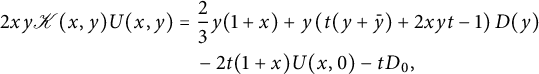 $$ \begin{align} 2 xy\mathscr K(x,y)U(x,y)&= \frac 2 3 y(1+x) +y\left(t(y+\bar y)+2xyt-1\right)D(y)\nonumber\\&\quad -2 t(1+x)U(x, 0)-tD_0, \end{align} $$
where $\mathscr K(x,y)=1-t\mathscr S(x,y)= 1-t(y+\bar y+xy+\bar x\bar y)$
is the kernel of Gessel’s model, reflected in the first diagonal. Compared with the original functional equation (2.14), the only thing that has changed is the initial term y, which has become
$\mathscr K(x,y)=1-t\mathscr S(x,y)= 1-t(y+\bar y+xy+\bar x\bar y)$
is the kernel of Gessel’s model, reflected in the first diagonal. Compared with the original functional equation (2.14), the only thing that has changed is the initial term y, which has become $2 y(1+x) /3$
.
$2 y(1+x) /3$
.
For the model $\mathscr S$
, we know two pairs of invariants (see Table 3): one is rational, and will not be used; the other takes the form (2.24) and involves quadrant generating functions:
$\mathscr S$
, we know two pairs of invariants (see Table 3): one is rational, and will not be used; the other takes the form (2.24) and involves quadrant generating functions:
 $$ \begin{align} \qquad I_1(x) =t(1+x)\mathscr Q( x,0)-\frac x{t(1+x)}, \qquad J_1(y)= -t \mathscr Q(0,y)+ t\mathscr Q_{0, 0}-\bar y. \hspace{-20pt}\end{align} $$
These two series are algebraic, and we refer to [Reference Bostan and Kauers5, Reference Bousquet-Mélou8] for explicit expressions. Denoting by $(I_1^g(x), J_1^g(y))$
the pair of invariants (8.5) that we used for Gessel walks, we observe that
$(I_1^g(x), J_1^g(y))$
the pair of invariants (8.5) that we used for Gessel walks, we observe that
 $$\begin{align*}I_1(x)=-J_1^g(x)+ t \mathscr Q_{0,0}, \qquad J_1(y)=- I_1^g(y)+ t \mathscr Q_{0,0}, \end{align*}$$
in accordance with the fact that the two models differ by an $x/y$
-symmetry.
$x/y$
-symmetry.
Theorem 8.5 Let $\mathcal S=\{\nearrow , \nwarrow , \swarrow , \searrow \}$
, and let
$\mathcal S=\{\nearrow , \nwarrow , \swarrow , \searrow \}$
, and let $\mathscr S= \{\uparrow , \nearrow , \downarrow , \swarrow \}$
be the set of reflected Gessel’s steps. Let
$\mathscr S= \{\uparrow , \nearrow , \downarrow , \swarrow \}$
be the set of reflected Gessel’s steps. Let $C(x,y)$
be the generating function of walks with steps in
$C(x,y)$
be the generating function of walks with steps in $\mathcal S$
, confined to the three-quadrant cone
$\mathcal S$
, confined to the three-quadrant cone $\mathcal {C}$
. Let us define
$\mathcal {C}$
. Let us define $A(x,y)$
as (8.1).
$A(x,y)$
as (8.1).
Let $I_1(x)$
and
$I_1(x)$
and $J_1(y)$
be the quadrant
$J_1(y)$
be the quadrant $\mathscr S$
-invariants defined by (8.15). The generating function
$\mathscr S$
-invariants defined by (8.15). The generating function $A(x,y)$
, which counts (weighted) walks in
$A(x,y)$
, which counts (weighted) walks in $\mathcal {C}$
with steps in
$\mathcal {C}$
with steps in $\mathcal S$
, satisfies equation (8.12), where
$\mathcal S$
, satisfies equation (8.12), where $A_-(x)$
can be expressed in terms of
$A_-(x)$
can be expressed in terms of $I_1$
and
$I_1$
and $J_1$
by
$J_1$
by
 $$ \begin{align} \frac 9 4 \left(2 t (\bar x+1) A_-(\sqrt x) +tD_{0} -\frac 2{3t(1+x)} \right) ^{2} = \big(I_1(x)- J_1(Y_0)\big)\big(I_1(x)- J_1(Y_1)\big). \end{align} $$
In this expression, the series $Y_{0,1}$
are the two roots of
$Y_{0,1}$
are the two roots of
 $$ \begin{align} \Delta(y)= \left(1-t^2\bar y (1+y)^2\right)\left(1-t^2\bar y (1-y)^2\right) \end{align} $$
that are formal power series in t.
The generating function $D(y)$
defined by (8.13) satisfies
$D(y)$
defined by (8.13) satisfies
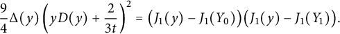 $$ \begin{align} \frac 9 4 {\Delta(y) } \left( yD ( y) +\frac {2}{3t} \right) ^{2} = \big(J_1(y)- J_1(Y_0)\big)\big(J_1(y)- J_1(Y_1)\big). \end{align} $$
In particular, the series $D_0=D(0)$
involved in (8.16) satisfies
$D_0=D(0)$
involved in (8.16) satisfies
 $$\begin{align*}3 t^2 D_0= 2+ t(J_1(Y_0)+ J_1(Y_1)). \end{align*}$$
The series $A_-(x)$
,
$A_-(x)$
, $D(y)$
, and
$D(y)$
, and $A(x,y)$
are algebraic.
$A(x,y)$
are algebraic.
Remark 8.6
Degrees and rational parametrizations of $A_-(\sqrt x)$
and
$A_-(\sqrt x)$
and $D(y)$
. We observe for this model the same phenomenon as for the simple model: the series
$D(y)$
. We observe for this model the same phenomenon as for the simple model: the series $\mathscr Q(x,0)$
and
$\mathscr Q(x,0)$
and $\mathscr Q(0,y)$
have degree
$\mathscr Q(0,y)$
have degree $24$
, but
$24$
, but $A_-(\sqrt x)$
and
$A_-(\sqrt x)$
and $D(y)$
have also degree
$D(y)$
have also degree $24$
(only). More precisely, using again the results and notation of [Reference Bousquet-Mélou8], one can express
$24$
(only). More precisely, using again the results and notation of [Reference Bousquet-Mélou8], one can express $\mathscr Q(x,0)$
and
$\mathscr Q(x,0)$
and $\mathscr Q(0,yt)$
(involved in the expressions of
$\mathscr Q(0,yt)$
(involved in the expressions of $I_1(x)$
and
$I_1(x)$
and $J_1(yt)$
, respectively) as rational functions in the four algebraic series T,
$J_1(yt)$
, respectively) as rational functions in the four algebraic series T, $Z=\sqrt T$
,
$Z=\sqrt T$
, $U\equiv U(y)$
, and
$U\equiv U(y)$
, and $V\equiv V(x)$
(note the exchange of x and y, which comes from the diagonal reflection of steps). One then derives from these results rational expressions of
$V\equiv V(x)$
(note the exchange of x and y, which comes from the diagonal reflection of steps). One then derives from these results rational expressions of $I_1(x)/t$
and
$I_1(x)/t$
and $J_1(yt)/t$
in terms of
$J_1(yt)/t$
in terms of $\sqrt T$
, U, and V, as well as the following expressions:
$\sqrt T$
, U, and V, as well as the following expressions:
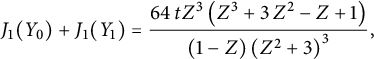 $$\begin{align*}J_1(Y_0)+J_1(Y_1)= {\frac {64\,t{Z}^{3} \left( {Z}^{3}+3\,{Z}^{2}-Z+1 \right) }{ \left(1- Z \right) \left( {Z}^{2}+3 \right) ^{3}}} , \end{align*}$$
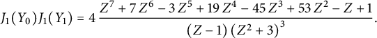 $$\begin{align*}J_1(Y_0)J_1(Y_1)= 4\,{\frac {{Z}^{7}+7\,{Z}^{6}-3\,{Z}^{5}+19\,{Z}^{4}-45\,{Z}^{3}+53\,{ Z}^{2}-Z+1}{ \left( Z-1 \right) \left( {Z}^{2}+3 \right) ^{3}}}. \end{align*}$$
Details of these calculations are given in our Maple session. Using (8.16) (resp. (8.18)), we then obtain a rational expression of
 $$\begin{align*}2 (\bar x+1) A_-(\sqrt x) +D_{0} -\frac 2{3t^2(1+x)} \qquad\left( \text{resp.} \quad D ( yt) +\frac {2}{3t^2y} \right) \end{align*}$$
of the form $\sqrt T \operatorname {\mathrm {Rat}}(T,V(x))$
(resp.
$\sqrt T \operatorname {\mathrm {Rat}}(T,V(x))$
(resp. $\sqrt T \operatorname {\mathrm {Rat}}(T,U(y))$
).
$\sqrt T \operatorname {\mathrm {Rat}}(T,U(y))$
).
Proof of Theorem 8.5
We start from the functional equation (8.14), and observe that we have a decoupling relation:
 $$\begin{align*}y (1+x) = (t(y+\bar y) +2txy-1)G(y)+F(x) + H(x,y) \mathscr K(x,y), \end{align*}$$
where
 $$\begin{align*}F(x)=\frac 1 {t(1+x)}, \qquad G(y)= \frac 1 t, \qquad H(x,y)=\frac x {t(1+x)}. \end{align*}$$
This, together with Lemma 2.3, leads us to define a new pair of invariants:
 $$\begin{align*}I(x)= \left(2 t(1+x) U(x,0) + tD_0-\frac 2 {3t(1+x)}\right)^2, \qquad J(y)= \Delta(y) \left(yD(y) + \frac{2}{3t}\right)^2, \end{align*}$$
where $\Delta (y)$
is given by (8.17). We want to combine them polynomially with the invariants
$\Delta (y)$
is given by (8.17). We want to combine them polynomially with the invariants $(I_1(x), J_1(y))$
given by (8.15) to form a pair of invariants
$(I_1(x), J_1(y))$
given by (8.15) to form a pair of invariants $(\tilde I(x), \tilde J(y))$
to which Lemma 2.6 applies.
$(\tilde I(x), \tilde J(y))$
to which Lemma 2.6 applies.
Observe that $I_1(x)$
and
$I_1(x)$
and $I(x)$
have poles at
$I(x)$
have poles at $x=-1$
, whereas
$x=-1$
, whereas $J_1(y)$
and
$J_1(y)$
and $J(y) $
have poles at
$J(y) $
have poles at $y=0$
. More precisely, the series
$y=0$
. More precisely, the series $J(y)$
has a (double) pole at
$J(y)$
has a (double) pole at $0$
, which can be removed by subtracting a well-chosen quadratic polynomial in
$0$
, which can be removed by subtracting a well-chosen quadratic polynomial in $J_1(y)$
. This leads us to introduce
$J_1(y)$
. This leads us to introduce
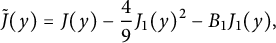 $$\begin{align*}\tilde J(y) = J(y) - \frac 4 9 J_1(y)^2 - B_1 J_1(y), \end{align*}$$
and to define accordingly
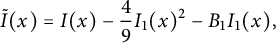 $$\begin{align*}\tilde I(x) = I(x) - \frac 4 9 I_1(x)^2 - B_1 I_1(x), \end{align*}$$
for a series $B_1$
that involves
$B_1$
that involves $D_0$
(we refer to our Maple session for details). Then, we use the functional equations satisfied by
$D_0$
(we refer to our Maple session for details). Then, we use the functional equations satisfied by $U(x,y)$
and
$U(x,y)$
and $\mathscr Q(x,y)$
to check that the ratio
$\mathscr Q(x,y)$
to check that the ratio
 $$\begin{align*}\frac{\tilde I(x) -\tilde J(y)}{\mathscr K(x,y)} \end{align*}$$
is a multiple of $xy$
, and conclude that
$xy$
, and conclude that $ \tilde I(x)= \tilde J(y)=B_0$
, for some series
$ \tilde I(x)= \tilde J(y)=B_0$
, for some series $B_0\in \mathbb {Q}((t))$
. Hence, denoting by
$B_0\in \mathbb {Q}((t))$
. Hence, denoting by $P(u)= 4u^2/9+B_1u+B_0$
, we have
$P(u)= 4u^2/9+B_1u+B_0$
, we have
 $$\begin{align*}I(x)= P(I_1(x)), \qquad J(y)= P(J_1(y)). \end{align*}$$
We can express the roots of P in terms of the series $\mathscr Q$
(and more precisely, in terms of
$\mathscr Q$
(and more precisely, in terms of $J_1$
) by looking at the two roots of
$J_1$
) by looking at the two roots of $\Delta (y)$
, denoted by
$\Delta (y)$
, denoted by $Y_i$
, with
$Y_i$
, with $i={0,1}$
, that lie in
$i={0,1}$
, that lie in $\mathbb {Q}[[t]]$
. For each of them,
$\mathbb {Q}[[t]]$
. For each of them, $J_1(Y_i)$
is a root of
$J_1(Y_i)$
is a root of $P(u)$
. This gives the expressions of the theorem, which are those of
$P(u)$
. This gives the expressions of the theorem, which are those of $9I(x)/4$
and
$9I(x)/4$
and $9J(y)/4$
.
$9J(y)/4$
.
Let us finish with the harmonic function associated with diagonal walks in $\mathcal {C}$
(known to be unique by [Reference Mustapha and Sifi29]).
$\mathcal {C}$
(known to be unique by [Reference Mustapha and Sifi29]).
Corollary 8.7 For $(i,j) \in \mathcal C$
, there exists a positive constant
$(i,j) \in \mathcal C$
, there exists a positive constant $H_{i,j}$
such that, as
$H_{i,j}$
such that, as $n\rightarrow \infty $
with
$n\rightarrow \infty $
with $n\equiv i+j\ \mod 2$
,
$n\equiv i+j\ \mod 2$
,
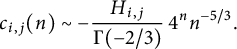 $$\begin{align*}c_{i,j}(n) \sim -\frac{H_{i,j}}{\Gamma(-2/3)}\, 4^n n^{-5/3}. \end{align*}$$
Clearly, $H_{i,j}=0$
if
$H_{i,j}=0$
if $i\not \equiv j$
mod
$i\not \equiv j$
mod $2$
. The generating function
$2$
. The generating function
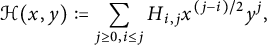 $$\begin{align*}\mathcal H(x,y):=\sum_{j\ge 0, i\le j} H_{i,j} x^{(j-i)/2} y^j, \end{align*}$$
which is a formal power series in x and y, is algebraic of degree $9$
, given by
$9$
, given by
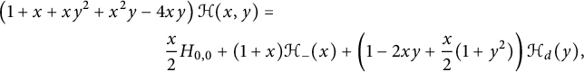 $$ \begin{align*} &\left(1+x+xy^2+x^2y-4xy\right) \mathcal H(x,y)= \\ &\phantom{1+x+xy^2+x^2y-4x} \frac x 2 H_{0,0} +(1+x)\mathcal H_-(x)+\left(1-2xy+\frac{x}2 (1+y^2)\right) \mathcal H_d(y), \end{align*} $$
where
 $$\begin{align*}\mathcal H_-(x):=\sum_{i>0} H_{-i,0} x^{i/2}\qquad \text{and} \qquad \mathcal H_d(y):=\sum_{i\ge 0} H_{i,i}y^i. \end{align*}$$
Each of these series is algebraic of degree $3$
. Let
$3$
. Let $ L(x)$
and
$ L(x)$
and $P(y)$
be defined as in Corollary 8.3. Then
$P(y)$
be defined as in Corollary 8.3. Then
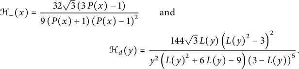 $$ \begin{align*} \mathcal H_-(x) &={\frac {32 \sqrt {3} \left( 3\,P(x)-1 \right) }{ 9\left( P(x)+1 \right) \left( P(x)-1 \right) ^{2}}} \qquad \text{and} \\ &\qquad \qquad\qquad\qquad \mathcal H_d(y) = {\frac {144\sqrt {3}\, L(y) \left( {L(y)}^{2}-3 \right) ^{2}}{y^2 \left( {L(y)}^{2 }+6\,L(y)-9 \right) \left( 3-L(y)\right) ^{5}}}. \end{align*} $$
(The exchange of x and y is intentional.)
Proof As in the proof of Corollary 8.3, one starts from the rational expressions of $A_-(\sqrt x)$
and
$A_-(\sqrt x)$
and $D(y)$
in terms of
$D(y)$
in terms of $\sqrt T$
,
$\sqrt T$
, $U(y)$
and
$U(y)$
and $V(x)$
derived from Theorem 8.5 and [Reference Bousquet-Mélou8], and then plugs in them the singular expansions of T,
$V(x)$
derived from Theorem 8.5 and [Reference Bousquet-Mélou8], and then plugs in them the singular expansions of T, $U(y)$
, and
$U(y)$
, and $V(x)$
around
$V(x)$
around $t^2=1/16$
. This gives
$t^2=1/16$
. This gives $\mathcal H_-(x)$
and
$\mathcal H_-(x)$
and $\mathcal H_d(y)$
. The expression of
$\mathcal H_d(y)$
. The expression of $\mathcal H(x,y)$
simply comes from the harmonicity of
$\mathcal H(x,y)$
simply comes from the harmonicity of $H_{i,j}$
.
$H_{i,j}$
.
9 Discussion and perspectives
9.1 Generic form of the results
For the last three models that we have solved ( $6$
th model of Table 1 in Section 7, and simple and diagonal models in Section 8), we have directly written the invariant
$6$
th model of Table 1 in Section 7, and simple and diagonal models in Section 8), we have directly written the invariant $I(x)$
, involving
$I(x)$
, involving $C_-(x)$
or
$C_-(x)$
or $A_-(x)$
, as a rational function in the quadrant invariant
$A_-(x)$
, as a rational function in the quadrant invariant $I_1(x)$
involving
$I_1(x)$
involving $\mathscr Q(x,0)$
; and analogously for
$\mathscr Q(x,0)$
; and analogously for $J(y)$
and
$J(y)$
and $J_1(y)$
(see Theorems 7.1, 8.1, and 8.5). The coefficients of these rational functions are series in t. This is also possible for the three models of the Kreweras trilogy, although we have (sometimes) also used the pair
$J_1(y)$
(see Theorems 7.1, 8.1, and 8.5). The coefficients of these rational functions are series in t. This is also possible for the three models of the Kreweras trilogy, although we have (sometimes) also used the pair $(I_0(x), J_0(y))$
to determine
$(I_0(x), J_0(y))$
to determine $(I(x),J(y))$
. For the Kreweras model and the reverse Kreweras model,
$(I(x),J(y))$
. For the Kreweras model and the reverse Kreweras model, $I(x)$
is a polynomial in
$I(x)$
is a polynomial in $I_1(x)$
(see (4.4) and (5.19)). For the double Kreweras model, one can ignore the pair
$I_1(x)$
(see (4.4) and (5.19)). For the double Kreweras model, one can ignore the pair $(I_0(x), J_0(y))$
as well, and prove that
$(I_0(x), J_0(y))$
as well, and prove that
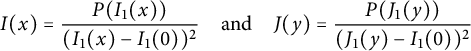 $$\begin{align*}I(x)= \frac{P(I_1(x))}{(I_1(x)-I_1(0))^2} \quad \text{and} \quad J(y)= \frac{P(J_1(y))}{(J_1(y)-I_1(0))^2} \end{align*}$$
for some polynomial $P(u)$
of degree
$P(u)$
of degree $4$
.
$4$
.
9.2 Solving more models via invariants?
Let us finally discuss if, and how, one could go further in the solution of three-quadrant walks using the approach of this paper. Let us first recall that this approach, when it works, relates invariants involving $C(x,y)$
to pre-existing invariants (or to weak invariants, in the sense of [Reference Bernardi, Bousquet-Mélou and Raschel2]), which so far are systematically D-algebraic. Hence, there is little hope to solve with this approach models that would not be (at least) D-algebraic. This means that for the nine models of Table 1, invariants have done for us all that we could hope for: they have solved the six models that were not already known to be hypertranscendental (that is, non-D-algebraic).
$C(x,y)$
to pre-existing invariants (or to weak invariants, in the sense of [Reference Bernardi, Bousquet-Mélou and Raschel2]), which so far are systematically D-algebraic. Hence, there is little hope to solve with this approach models that would not be (at least) D-algebraic. This means that for the nine models of Table 1, invariants have done for us all that we could hope for: they have solved the six models that were not already known to be hypertranscendental (that is, non-D-algebraic).
If we want to go further, two different difficulties arise: the model may contain NW and/or SE steps, and it may not be diagonally symmetric. Let us consider two examples.
Diagonally symmetric models with NW and SE steps
Apart from the diagonal model, which we have actually solved via invariants, there are eight models in this class, as shown in Table 6. The first two are associated with a finite group (orders $4$
and
$4$
and $6$
) and the other six with an infinite group. Let us consider, for instance, the fourth model of the table,
$6$
) and the other six with an infinite group. Let us consider, for instance, the fourth model of the table, $\mathcal S=\{\nearrow , \nwarrow , \leftarrow , \downarrow , \searrow \}$
(the scarecrow), and write as before
$\mathcal S=\{\nearrow , \nwarrow , \leftarrow , \downarrow , \searrow \}$
(the scarecrow), and write as before
 $$\begin{align*}C(x,y)=\bar x U(\bar x, xy)+ D(xy)+ \bar y U(\bar y,xy), \end{align*}$$
with $D(y) \in \mathbb {Q}[y][[t]]$
and
$D(y) \in \mathbb {Q}[y][[t]]$
and $U(x,y) \in \mathbb {Q} [x,y][[t]]$
.
$U(x,y) \in \mathbb {Q} [x,y][[t]]$
.
Table 6: The nine models with $x/y$
-symmetry and steps
$x/y$
-symmetry and steps $\nwarrow $
and
$\nwarrow $
and $\searrow $
. The first three have a finite group and are Weyl models in the sense of [Reference Bousquet-Mélou and Wallner12]; the others have an infinite group.
$\searrow $
. The first three have a finite group and are Weyl models in the sense of [Reference Bousquet-Mélou and Wallner12]; the others have an infinite group.
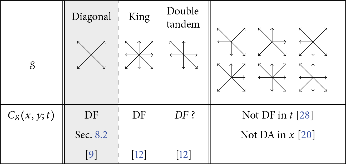
We can write functional equations, first for $D(xy)$
and
$D(xy)$
and $\bar x U(\bar x,xy)$
, as we did in Section 2.1. A step-by-step construction of walks gives
$\bar x U(\bar x,xy)$
, as we did in Section 2.1. A step-by-step construction of walks gives
 $$\begin{align*}D(xy) = 1+ t xy D(xy) +2t \bar y \left(\bar x U(0,xy)-\bar x U_{0,0}\right) + 2t x \bar y \left(\bar x^2 U_1(xy)-\bar x^2 U_{1,0}\right), \end{align*}$$
where $U_1(y)$
is the coefficient of x in
$U_1(y)$
is the coefficient of x in $U(x,y)$
. The term involving
$U(x,y)$
. The term involving $U_1$
is new, and corresponds to walks that jump from the lines
$U_1$
is new, and corresponds to walks that jump from the lines $j-i=\pm 2$
to the diagonal, using an NW of SE step. For walks ending above the diagonal, we find
$j-i=\pm 2$
to the diagonal, using an NW of SE step. For walks ending above the diagonal, we find
 $$ \begin{align*} &\bar x \left(1- tS(x,y)\right) U(\bar x,xy)= t \bar x (1+y) D(xy)+ t\bar x y \left(\bar y U(0,xy)-\bar y U_{0,0}\right)\\ &\qquad -t \bar y (1+x) \left(\bar x U(\bar x,0)+ \bar x U(0,xy) -\bar x U_{0,0}\right) -tx\bar y \left(\bar x^2 U_1(xy)-\bar x^2 U_{1,0}\right), \end{align*} $$
with $S(x,y)=xy+\bar x y +\bar x +\bar y +x\bar y$
. The second term on the first line accounts for walks jumping from the line
$S(x,y)=xy+\bar x y +\bar x +\bar y +x\bar y$
. The second term on the first line accounts for walks jumping from the line $j=i-1$
to the line
$j=i-1$
to the line $j=i+1$
by an NW step (we forbid steps from
$j=i+1$
by an NW step (we forbid steps from $(0,-1)$
to
$(0,-1)$
to $(-1,0)$
). The last term of the second line accounts for walks that would jump from the line
$(-1,0)$
). The last term of the second line accounts for walks that would jump from the line $j=i+2$
to the diagonal.
$j=i+2$
to the diagonal.
We can eliminate the series $U_1(xy)$
by taking a linear combination of the two equations; but we still have
$U_1(xy)$
by taking a linear combination of the two equations; but we still have $U(0,xy)$
and
$U(0,xy)$
and $D(xy)$
, while we only had one of them when the steps NW and SE were forbidden. Upon performing the change of variables
$D(xy)$
, while we only had one of them when the steps NW and SE were forbidden. Upon performing the change of variables $(x,y )\mapsto ( \bar x, xy)$
, we finally obtain the following counterpart of (2.12):
$(x,y )\mapsto ( \bar x, xy)$
, we finally obtain the following counterpart of (2.12):
 $$ \begin{align*} 2xy \mathscr K(x,y) U(x,y)&= y + y\, \big(t y+ 2tx (1+xy) -1\big) D(y)\\ &\qquad\quad -2t (1+\bar x) U(x,0) + 2t(xy-\bar x) \left( U(0,y)-U_{0,0}\right), \end{align*} $$
with $\mathscr K(x,y):=1-tS(\bar x,xy)= 1-t (x+ \bar x \bar y +y +\bar x^2 \bar y +x^2 y)$
. The main two novelties are the facts that the kernel has degree
$\mathscr K(x,y):=1-tS(\bar x,xy)= 1-t (x+ \bar x \bar y +y +\bar x^2 \bar y +x^2 y)$
. The main two novelties are the facts that the kernel has degree $2$
and valuation
$2$
and valuation $-2$
in x, and that the right-hand side involves two series in y, namely
$-2$
in x, and that the right-hand side involves two series in y, namely $D(y)$
and
$D(y)$
and $U(0,y)$
. Hence, it seems that the first step toward solving this three-quadrant model via invariants would be to learn how to solve quadrant models with large steps via invariants—a question already raised in [Reference Bostan, Bousquet-Mélou and Melczer3].
$U(0,y)$
. Hence, it seems that the first step toward solving this three-quadrant model via invariants would be to learn how to solve quadrant models with large steps via invariants—a question already raised in [Reference Bostan, Bousquet-Mélou and Melczer3].
Asymmetric models
There are $74-8-9=57$
models that do not have the
$74-8-9=57$
models that do not have the $x/y$
-symmetry. Exactly
$x/y$
-symmetry. Exactly $16$
have a finite group, among which
$16$
have a finite group, among which $4$
(at least) are conjectured to have a D-finite (even algebraic, in one case) generating function [Reference Bousquet-Mélou and Wallner12]. They are shown in Table 7.
$4$
(at least) are conjectured to have a D-finite (even algebraic, in one case) generating function [Reference Bousquet-Mélou and Wallner12]. They are shown in Table 7.
Table 7: Four interesting asymmetric models with a finite group. The first three are Weyl models in the sense of [Reference Bousquet-Mélou and Wallner12].
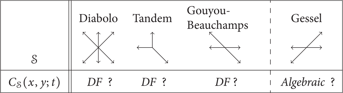
To illustrate the new difficulties that arise, let us work out functional equations for Gessel’s model. Since symmetry is lost, we now write
 $$\begin{align*}C(x,y)=\bar x U(\bar x, xy)+ D(xy)+ \bar y L(\bar y,xy),\\[-14pt] \end{align*}$$
with $D(y) \in \mathbb {Q}[y][[t]]$
and
$D(y) \in \mathbb {Q}[y][[t]]$
and $U(x,y)$
,
$U(x,y)$
, $L(x,y) \in \mathbb {Q} [x,y][[t]]$
. The equation for walks ending on the diagonal reads
$L(x,y) \in \mathbb {Q} [x,y][[t]]$
. The equation for walks ending on the diagonal reads
 $$\begin{align*}\left(1-t (xy+\bar x\bar y) \right)D(xy)=1- t\bar x\bar y D_0+ tx\left( \bar x U(0, xy) \right)+ t \bar x\left( \bar y L(0,xy)-\bar y L_{0,0}\right).\\[-14pt] \end{align*}$$
Now, for walks ending above the diagonal, we obtain
 $$\begin{align*}\left( 1-t S(x,y)\right) \bar x U(\bar x,xy)= t\bar x D(xy) - t\bar x \bar y \left(\bar x U(\bar x,0)\right) -tx \left(\bar x U(0,xy)\right),\\[-14pt] \end{align*}$$
with $S(x,y)=x+\bar x +xy+\bar x\bar y$
. Finally, for walks ending below the diagonal, we find
$S(x,y)=x+\bar x +xy+\bar x\bar y$
. Finally, for walks ending below the diagonal, we find
 $$\begin{align*}\left( 1-t S(x,y)\right) \bar y L(\bar y,xy) = tx D(xy)-t \bar x(1+\bar y) \bar y L(\bar y,0) -t\bar x \left(\bar y L(0,xy)- \bar y L_{0,0}\right).\\[-14pt] \end{align*}$$
In the first two equations, we perform the same change of variables as before, namely $(x,y) \mapsto (\bar x, xy)$
. In the third equation, we apply
$(x,y) \mapsto (\bar x, xy)$
. In the third equation, we apply $( x,y)\mapsto (xy, \bar x) $
. This gives
$( x,y)\mapsto (xy, \bar x) $
. This gives
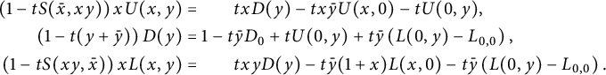 $$ \begin{align*} \left( 1-t S(\bar x,xy)\right) x U(x,y)&= \hskip 6mm tx D(y) - tx \bar y U(x,0) -t U(0,y), \\ \left(1-t (y+\bar y) \right)D(y)&=1- t\bar y D_0+ t U(0, y) + t \bar y \left(L(0,y)- L_{0,0}\right), \\ \left( 1-t S(xy,\bar x)\right) x L(x,y) &= \hskip 6mm txy D(y)-t \bar y(1+x) L(x,0) -t \bar y \left( L(0,y)- L_{0,0}\right).\\[-14pt] \end{align*} $$
We now have a system with two trivariate series $U(x,y)$
and
$U(x,y)$
and $L(x,y)$
. In addition, the kernels
$L(x,y)$
. In addition, the kernels
 $$\begin{align*}1-t S(\bar x,xy)= 1-t(x+\bar x+y+\bar y)\quad \text{ and } \quad 1-tS(xy,\bar x)=1-t(y+\bar y +xy+\bar x\bar y)\\[-14pt] \end{align*}$$
are not the same.
Acknowledgment
I am grateful to Kilian Raschel for several interesting discussions on discrete harmonic functions.


 Open access