


1. Introduction
Turbulent, dispersed, multiphase flows are not yet fully understood due to their complex, multiscale dynamics. The dispersed phase may consist of solid inertial particles, bubbles or gases and their interaction with the carrier fluid depends on a number of factors including their density (relative to the fluid density), their total mass (relative to the total fluid mass) and the nature of the turbulence. Despite their complexity, experimental, computational and theoretical investigations have made significant progress in understanding various aspects of such flows, including the dispersion and clustering of particles, droplet breakdown and coalescence and turbulent modulation (see Balachandar & Eaton (Reference Balachandar and Eaton2010), Gustavsson & Mehlig (Reference Gustavsson and Mehlig2016), Brandt & Coletti (Reference Brandt and Coletti2022) and Bec, Gustavsson & Mehlig (Reference Bec, Gustavsson and Mehlig2024), for reviews). This has led to advances in our understanding of diverse problems including cloud microphysics (Pruppacher & Klett Reference Pruppacher and Klett1997; Shaw Reference Shaw2003), aerosol deposition in human lungs (Ou, Jian & Deng Reference Ou, Jian and Deng2020) and planetesimal formation (Cuzzi et al. Reference Cuzzi, Hogan, Paque and Dobrovolskis2000; Birnstiel, Fang & Johansen Reference Birnstiel, Fang and Johansen2016).
We focus on the problem of the settling velocity of inertial particles in isotropic turbulence for particles that are small compared with the Kolmogorov length scale, and are much denser than the fluid. Many experimental and numerical studies have observed that such inertial particles settle faster in a turbulent flow than they would in a quiescent fluid (Wang & Maxey Reference Wang and Maxey1993; Aliseda et al. Reference Aliseda, Cartellier, Hainaux and Lasheras2002; Yang & Shy Reference Yang and Shy2005; Bec, Homann & Ray Reference Bec, Homann and Ray2014; Good et al. Reference Good, Ireland, Bewley, Bodenschatz, Collins and Warhaft2014; Rosa et al. Reference Rosa, Parishani, Ayala and Wang2016; Monchaux & Dejoan Reference Monchaux and Dejoan2017; Dhariwal & Bragg Reference Dhariwal and Bragg2019; Momenifar, Dhariwal & Bragg Reference Momenifar, Dhariwal and Bragg2019; Petersen, Baker & Coletti Reference Petersen, Baker and Coletti2019; Momenifar & Bragg Reference Momenifar and Bragg2020; Berk & Coletti Reference Berk and Coletti2021). Prior to these observations, it had also been shown by Maxey & Corrsin (Reference Maxey and Corrsin1986) that, in random flow fields, inertial particles settle faster than they would in a quiescent flow. Maxey (Reference Maxey1987) proposed the preferential sweeping mechanism to explain how turbulence (or fluctuations in a random flow) could cause inertial particles to settle faster than they would in a quiescent flow. In particular, Maxey argued that, for weakly inertial settling particles, the combined effects of the structure of the strain-rate and vorticity fields of the flow, particle inertia and gravity cause the particles to be preferentially swept around the downward moving side of vortices in the flow. Hence, the average fluid velocity along their trajectory points down, leading to an enhancement of their settling velocity. Recently, Tom & Bragg (Reference Tom and Bragg2019) extended the analysis of Maxey (Reference Maxey1987) to explain how the preferential sweeping mechanism works when the particle inertia is finite, and examined the role that different turbulent flow scales play in the mechanism. This was called the multi-scale preferential sweeping mechanism and it successfully explained a number of previous results that could not be accounted for by the original analysis of Maxey (Reference Maxey1987).
Many of the studies mentioned above focused on the one-way coupled (1WC) regime, where the effect of the particles on the flow is ignored, in contrast to the two-way coupled (2WC) regime. Other studies have, however, considered the effect of 2WC on particle settling, including Bosse, Kleiser & Meiburg (Reference Bosse, Kleiser and Meiburg2006), Dejoan (Reference Dejoan2011), Monchaux & Dejoan (Reference Monchaux and Dejoan2017) and Rosa et al. (Reference Rosa, Kopeć, Ababaei and Pozorski2021, Reference Rosa, Kopeć, Ababaei and Pozorski2022). These studies all found that 2WC causes the particles to settle faster than the 1WC case. Bosse et al. (Reference Bosse, Kleiser and Meiburg2006) and Monchaux & Dejoan (Reference Monchaux and Dejoan2017) emphasised that the primary contribution to settling enhancement results from the augmented fluid velocity at the particle position induced by the collective particle back-reaction force. Indeed, Aliseda et al. (Reference Aliseda, Cartellier, Hainaux and Lasheras2002) observed increased mean particle settling enhancements in regions of higher local particle concentration, and Hassaini, Petersen & Coletti (Reference Hassaini, Petersen and Coletti2023) noted that larger clusters settle faster. Monchaux & Dejoan (Reference Monchaux and Dejoan2017) authors argued that the centrifuging mechanism decreases with increasing volume fraction in the presence of 2WC and that there is a monotonic decrease in preferential concentration with increasing volume fraction. On a related note, Hassaini et al. (Reference Hassaini, Petersen and Coletti2023) observed that clustering becomes more intense with increasing volume fraction. Tom, Carbone & Bragg (Reference Tom, Carbone and Bragg2022) investigated the issue of preferential sampling in greater detail, applying the multi-scale preferential sweeping mechanism developed in Tom & Bragg (Reference Tom and Bragg2019) to the 2WC case. In agreement with Monchaux & Dejoan (Reference Monchaux and Dejoan2017), Tom et al. (Reference Tom, Carbone and Bragg2022) found that 2WC can substantially increase the particle settling velocities compared with the 1WC case even in regimes where the particle mass loading is small enough for the effect of the particles on the global fluid statistics to be negligible. However, they argued that preferential sweeping continues to be the mechanism responsible for the enhanced settling speeds due to turbulence. In particular, they showed that the difference between the 1WC and 2WC cases is that, in the 2WC case, the particles are not merely swept around the downward moving side of vortices in the flow but they also drag the fluid down with them in these regions as they fall. Hence, the fluid dragging effect does not replace the preferential sweeping mechanism, but acts with it to further enhance the particle settling velocities compared with the 1WC case.
It is not yet understood to which extent the findings of previous studies (e.g. Bosse et al. Reference Bosse, Kleiser and Meiburg2006; Monchaux & Dejoan Reference Monchaux and Dejoan2017; Tom et al. Reference Tom, Carbone and Bragg2022) generalise over a wider portion of the parameter space. For example, while Tom et al. (Reference Tom, Carbone and Bragg2022) considered a range of Stokes numbers  $St\equiv \tau _p/\tau _\eta \in [0.3,2]$ (where $\tau _p$ is the particle response time and $\tau _\eta$ is the Kolmogorov time scale), it restricted attention to a single Froude number $Fr\equiv u_\eta /(\tau _\eta g)=1$ (where $u_\eta$ is the Kolmogorov velocity scale and $g$ is the gravitational acceleration) and volume fraction $\varPhi =1.5\times 10^{-5}$. The resulting mass loading was thus small enough for the particles to only weakly affect the global statistics of the flow. However, at mass loadings large enough for the particles to substantially modify the global statistics of the flow, the local structure of the flow in the vicinity of the particles may be so dramatically modified that the preferential sweeping mechanism (which is conceptualised in the 1WC limit) no longer applies. If the settling particles dramatically alter the velocity gradient field then it may no longer be the case that the particles are swept around the downward moving side of vortices in the flow as the structure of the vorticity field may be completely different and is no longer passive with respect to the particles. In the opposite limit, as the mass loading approaches zero, it is not obvious that the effect of 2WC on the particle settling should vanish. Although in this limit a vanishing portion of the flow directly feels the effect of the momentum coupling (such that the effect of 2WC on the global fluid statistics will vanish), it is only this vanishing portion of the flow that matters for the particle settling. This is because the force on the particle is only directly affected by the flow in the vicinity of the particle. This issue is important to explore since it is almost universally assumed that, in the limit of low mass loadings (low enough for the global fluid statistics to be unaffected by the particles), the effect of 2WC on the particle motion should be unimportant.
The rest of the paper is organised as follows: in § 2 we outline the problem of interest, in § 3 we summarise the numerical methods, in § 4 we present and discuss the observations of our simulations and in § 5 we compare our results with prior experiments and numerical studies. Finally, in § 6, we summarise our findings.
2. Problem formulation
We consider a dilute suspension (i.e. the volume fraction  $\varPhi _v$ is small enough to ignore particle collisions) of small ( $d_p/\eta \ll 1$, where $d_p$ is the particle diameter and $\eta$ is the Kolmogorov length scale), dense ( $\rho _p/\rho _f \gg 1$, where $\rho _p$ is the particle density and $\rho _f$ is the fluid density), spherical, inertial particles settling under the force of gravity. Such assumptions are often considered to be suitable for modelling droplet transport in atmospheric clouds (Shaw Reference Shaw2003; Grabowski & Wang Reference Grabowski and Wang2013), and dust transport in the atmosphere (Richter & Chamecki Reference Richter and Chamecki2018).
Assuming that the particle Reynolds number is small, the evolution equation for particles in this regime is given by (Maxey & Riley Reference Maxey and Riley1983)
 \begin{equation} \ddot{\boldsymbol{x}}^p(t)\equiv\dot{\boldsymbol{v}}^p(t)=\frac{1}{\tau_p} [\boldsymbol{u}(\boldsymbol{x}^p(t),t)-\boldsymbol{v}^p(t)]+\boldsymbol{g},\end{equation}
where  $\boldsymbol {x}^p(t)$ and $\boldsymbol {v}^p(t)$ denote the particle position and velocity, respectively, $\boldsymbol {u}(\boldsymbol {x}^p(t),t)$ is the undisturbed fluid velocity at the particle position, $\tau _\eta$ is the Kolmogorov time scale and $\boldsymbol {g}$ denotes the gravitational acceleration. The particle response time $\tau _p$ is given by
 \begin{equation} \tau_p = \frac{1}{18}\frac{\rho_p/\rho_f}{\nu} d_p^2, \end{equation}
where  $\nu$ is the dynamic viscosity.
The particles settle in a statistically stationary, homogeneous turbulent flow, which is governed by the incompressible Navier–Stokes equation (written here in rotational form)
 \begin{equation} \partial_t \boldsymbol{u} =\boldsymbol{u}\times\boldsymbol{\omega} -\boldsymbol{\nabla}\left(\frac{P}{\rho_f} + \frac{u^2}{2}\right) + \nu\nabla^2\boldsymbol{u} + \boldsymbol{F} + \boldsymbol{C},\quad \boldsymbol{\nabla}\boldsymbol{\cdot}\boldsymbol{u} = 0. \end{equation}
Here,  $\boldsymbol {u}(\boldsymbol {x},t)$ and $\boldsymbol {\omega }\equiv \boldsymbol {\nabla }\times \boldsymbol {u}$ are the fluid velocity and vorticity fields, respectively, $P(\boldsymbol {x},t)$ is the pressure, $\boldsymbol {C}(\boldsymbol {x},t)$ is the total momentum feedback of the particles on the carrier fluid and $\boldsymbol {F}(\boldsymbol {x},t)$ is the large-scale forcing required to maintain steady-state turbulence. In our direct numerical simulations (DNSs) we will consider the case where $\boldsymbol {F}$ isotropically forces the flow, such that, when $\boldsymbol {g}=\boldsymbol {0}$, the flow is statistically isotropic, but it is anisotropic for $\boldsymbol {g}\neq \boldsymbol {0}$ due to the momentum coupling term $\boldsymbol {C}$.
We consider the particle motion in both the 1WC scenario where we set  $\boldsymbol {C}=\boldsymbol {0}$, and the 2WC scenario where $\boldsymbol {C}\neq \boldsymbol {0}$. The particle feedback $\boldsymbol {C}$ is the sum of the hydrodynamic forces generated by all particles at location $\boldsymbol {x}^p(t)=\boldsymbol {x}$
 \begin{equation} \boldsymbol{C}(\boldsymbol{x},t)=\frac{1}{\rho_f}\sum_i \boldsymbol{f}_i^p(t) \delta(\boldsymbol{x}-\boldsymbol{x}^p_i(t)),\quad \boldsymbol{f}_i^p(t) =-\frac{m_p}{St\tau_\eta} [\boldsymbol{u}(\boldsymbol{x}^p_i(t),t)-\boldsymbol{v}^p_i(t)], \end{equation}
where  $m_p$ is the mass of each particle, $\boldsymbol {x}^p_i$ and $\boldsymbol {v}^p_i$ are the position and velocity of the $i$th particle and $\boldsymbol {f}^p_i$ is the reaction force generated by the $i$th particle. As discussed in Tom et al. (Reference Tom, Carbone and Bragg2022), when $\boldsymbol {C}\neq \boldsymbol {0}$, settling particles will generate a mean flow in the direction of $\boldsymbol {g}$. In order to generate a zero mean-flow velocity in the vertical direction, the pressure is accordingly modified, a method that was also used in Maxey & Patel (Reference Maxey and Patel2001), Bosse et al. (Reference Bosse, Kleiser and Meiburg2006), Monchaux & Dejoan (Reference Monchaux and Dejoan2017) and Rosa et al. (Reference Rosa, Kopeć, Ababaei and Pozorski2021).
The ensemble-averaged mean particle settling speed can be obtained from (2.1), assuming statistical homogeneity and stationarity
 \begin{equation} \langle{v}_z^p(t)\rangle=\langle{u}_z(\boldsymbol{x}^p(t),t)\rangle-St\tau_\eta{g}.\end{equation}
Here,  $St \tau _\eta g$ is the Stokes settling speed (the settling speed the particle would have in a quiescent fluid) and $\langle \boldsymbol {u}(\boldsymbol {x}^p(t),t) \rangle$ is the ensemble-average vertical fluid velocity at the particle location. It is this latter contribution that represents the contribution of turbulence to the settling speed. Even when the Eulerian average of the vertical fluid velocity is zero $\langle {u}_z(\boldsymbol {x},t)\rangle ={0}$, the average along the particle trajectory $\langle {u}_z(\boldsymbol {x}^p(t),t)\rangle$ need not be zero because inertial particles will not in general sample the flow field ergodically. As a result of this, through the contribution $\langle {u}_z(\boldsymbol {x}^p(t),t)\rangle$ turbulence can lead to either enhanced settling ( $\langle {v}_z^p(t)\rangle < -St\tau _\eta {g}$) or hindering ( $\langle {v}_z^p(t)\rangle > -St\tau _\eta {g}$). Results from laboratory experiments, field measurements and numerical simulations show that, for the case of small, dense, inertial particles, it is enhanced settling that has been predominantly observed (Wang & Maxey Reference Wang and Maxey1993; Yang & Shy Reference Yang and Shy2005; Bec et al. Reference Bec, Homann and Ray2014; Good et al. Reference Good, Ireland, Bewley, Bodenschatz, Collins and Warhaft2014; Ireland, Bragg & Collins Reference Ireland, Bragg and Collins2016; Rosa et al. Reference Rosa, Parishani, Ayala and Wang2016; Nemes et al. Reference Nemes, Dasari, Hong, Guala and Coletti2017; Petersen et al. Reference Petersen, Baker and Coletti2019; Li et al. Reference Li, Lim, Berk, Abraham, Heisel, Guala, Coletti and Hong2021a,Reference Li, Abraham, Guala and Hongb; Tom et al. Reference Tom, Carbone and Bragg2022).
3. Direct numerical simulations
3.1. Numerical method
We adopt an Eulerian–Lagrangian approach to numerically integrate (2.1) in conjunction with (2.3a,b). We perform DNS of statistically stationary, homogeneous turbulence in a three-dimensional, periodic domain using a pseudo-spectral scheme on  $N^3$ collocation points (Ireland et al. Reference Ireland, Vaithianathan, Sukheswalla, Ray and Collins2013). A second-order Runge–Kutta time-stepping scheme with an exponential integration is employed for the viscous stress, and a combination of spherical truncation and phase shifting for the dealiasing schemes. A seventh-order, B-spline polynomial interpolation scheme (that uses eight points) is used to calculate both the fluid velocities at the particle position and to project the particle-momentum feedback onto the fluid at the grid points. Equation (2.1) is solved using an exponential integrator method (Hochbruck & Ostermann Reference Hochbruck and Ostermann2010), which ensures stability and accuracy for low Stokes number particles while allowing the same time step to be used for both the fluid and particle equations of motion. We refer the reader to Ireland et al. (Reference Ireland, Vaithianathan, Sukheswalla, Ray and Collins2013) and Tom et al. (Reference Tom, Carbone and Bragg2022) for further details on the numerical solver, and Beylkin (Reference Beylkin1995) and Carbone, Bragg & Iovieno (Reference Carbone, Bragg and Iovieno2019) for the method for computing the momentum coupling term $\boldsymbol {C}$, and the interpolation schemes.
3.2. Simulation parameters
Table 1 summarises the parameters of our unladen DNS, where  $\mathcal {L}$ is the domain length, $N$ is the number of collocation points (the grid size is thus $N^3$) and $\nu$ is the viscosity. These same values are used for all of the 1WC and 2WC DNS cases. The table also shows turbulence statistics from the DNS of the unladen flow: the mean dissipation rate $\langle \epsilon \rangle$, the root mean square (r.m.s.) fluctuating velocity $u'\equiv \sqrt {2\mathcal {K}/3}$ (where $\mathcal {K}$ is the turbulent kinetic energy), the Kolmogorov velocity and length scales, $u_{\eta }$ and $\eta$, respectively, the integral length scale $L$ and the Taylor microscale Reynolds number $Re_{\lambda } \equiv u'\lambda /\nu$, where $\lambda$ is the Taylor length scale.
Table 1. Flow parameters in DNS for the unladen flow. Here,  $Re_{\lambda } \equiv u'\lambda /\nu = 2k/\sqrt {5/3\nu \langle \epsilon \rangle }$ is the Taylor microscale Reynolds number, $\lambda$ is the Taylor microscale, $\mathcal {L}$ is the domain length, $N$ is the number of grid points in each direction, $\nu$ is the fluid kinematic viscosity, $\langle \epsilon \rangle$ is the mean turbulent kinetic energy dissipation rate, $L$ is the integral length scale, $\eta \equiv (\nu ^{3}/\langle \epsilon \rangle )^{1/4}$ is the Kolmogorov length scale, $u' \equiv \sqrt {2\mathcal {K}/3}$ is the r.m.s. of the fluctuating fluid velocity, $\mathcal {K}$ is the turbulent kinetic energy, $u_{\eta }$ is the Kolmogorov velocity scale, $\tau _L \equiv L/u'$ is the large-eddy turnover time, $\tau _{\eta }$ is the Kolmogorov time scale, $k_{max} = \sqrt {2N/3}$ is the maximum resolved wavenumber and $dt$ is the time step. The small-scale resolution, $k_{max}\eta$ and the total flow kinetic energy measured by $u'$ are approximately constant between the different simulations. These flow statistics are constructed by averaging over the spatial domain and averaging over a time period of $10\tau _L$.
For the 1WC and 2WC simulations, the Stokes number  $St\equiv \tau _p/\tau _\eta$ and the Froude number $Fr\equiv u_\eta /(\tau _\eta g)$ are defined with respect to the unladen fluid statistics, and we consider Stokes numbers $St=0.3$, $0.5$, $0.7$, $1$,
$1$,  $2$ (referred to as $St_1$, $St_2$, $St_3$, $St_4$ and $St_5$, respectively), each of which is considered for three different Froude numbers $Fr=0.3$, $1$ and $3$ (referred to as $Fr_1$, $Fr_2$ and $Fr_3$, respectively). The particle mass loading $\varPhi _m$ is related to the volume fraction $\varPhi$ through
 \begin{equation}
\varPhi_m=\frac{\rho_p}{\rho_f}\varPhi=\frac{\rho_p}{\rho_f}
\frac{{\rm \pi} d_p^3}{6} \frac{N_p}{L^3},
\end{equation}
\begin{equation}
\varPhi_m=\frac{\rho_p}{\rho_f}\varPhi=\frac{\rho_p}{\rho_f}
\frac{{\rm \pi} d_p^3}{6} \frac{N_p}{L^3},
\end{equation}
and we consider particles with constant density  $\rho _p/\rho _f= 5000$, the same as that used in Bosse et al. (Reference Bosse, Kleiser and Meiburg2006), Monchaux & Dejoan (Reference Monchaux and Dejoan2017) and Tom et al. (Reference Tom, Carbone and Bragg2022). Since $\rho _p/\rho _f$ is fixed, varying $\varPhi _m$ corresponds to varying $\varPhi$, and therefore we will often refer to the effect of varying $\varPhi$ even though strictly speaking the momentum coupling depends on $\varPhi _m$ and not simply $\varPhi$. For each choice of $St$ and $Fr$, we consider $\varPhi = 1.5\times 10^{-6}$, $7\times 10^{-6}$, $1.5\times 10^{-5}$, $7\times 10^{-5}$ and $1.5\times 10^{-4}$, which we refer to as $\varPhi _1,\varPhi _2,\varPhi _3,\varPhi _4,\varPhi _5$, respectively. However, due to computational resources, we were unable to complete the run with $St=2, Fr=0.3, \varPhi =1.5\times 10^{-4}$. This makes for a total of 59 different DNS, and due to this we are restricted to cases where the unladen flow has $Re_{\lambda } \simeq 88$. The present study significantly expands on the study of Tom et al. (Reference Tom, Carbone and Bragg2022), where only $Fr=1$ and $\varPhi = 1.5\times 10^{-5}$ were considered, for the same $St$ and $Re_\lambda$ values.
3.3. Simulation approach
The DNS of the unladen flow were run for approximately 20  $\tau _L$ until a statistically stationary state was reached. For the 1WC runs, the DNS were initialised using the fluid data obtained at the final time step of the unladen DNS, and using random initial particle positions and initial particle velocities equal to the local fluid velocity plus the Stokes settling velocity. For the 2WC simulations, the DNS were initialised using the fluid and particle data obtained at the final time step of the corresponding 1WC DNS (i.e. having the same $St, Fr, \varPhi$). For both the 1WC and 2WC simulations, we collected statistics over a period of 60 $\tau _L$ to ensure reasonable statistical convergence (this is a smaller window than that used in Tom et al. (Reference Tom, Carbone and Bragg2022) but tests showed that it was sufficient). A summary of the key fluid statistics and the parameters from all of the 2WC runs is provided in table 3 in the Appendix for reference.
4. Results
4.1. Discussion on fluid statistics
Before we explore the parametric dependence of the impact of 2WC on the particle dynamics in turbulence, it is informative to first consider how 2WC affects the global flow statistics. We first consider the probability density function (PDF)  $\mathcal {P}(\mathcal {Q})\equiv \langle \delta (Q(\boldsymbol {x},t)-\mathcal {Q}\rangle$, where $\boldsymbol {x}$ denotes a fixed point in the flow, $Q$ is the second invariant of the velocity gradient tensor $\boldsymbol{\mathsf{A}}$
 \begin{equation}
Q \equiv
\boldsymbol{\mathsf{S}}\boldsymbol{:}\boldsymbol{\mathsf{S}}-\boldsymbol{\mathsf{R}}\boldsymbol{:}\boldsymbol{\mathsf{R}}; \quad
\boldsymbol{\mathsf{S}}\equiv(\boldsymbol{\mathsf{A}}+\boldsymbol{\mathsf{A}}^\top)/2,\quad
\boldsymbol{\mathsf{R}}\equiv(\boldsymbol{\mathsf{A}}-\boldsymbol{\mathsf{A}}^\top)/2,
\end{equation}
\begin{equation}
Q \equiv
\boldsymbol{\mathsf{S}}\boldsymbol{:}\boldsymbol{\mathsf{S}}-\boldsymbol{\mathsf{R}}\boldsymbol{:}\boldsymbol{\mathsf{R}}; \quad
\boldsymbol{\mathsf{S}}\equiv(\boldsymbol{\mathsf{A}}+\boldsymbol{\mathsf{A}}^\top)/2,\quad
\boldsymbol{\mathsf{R}}\equiv(\boldsymbol{\mathsf{A}}-\boldsymbol{\mathsf{A}}^\top)/2,
\end{equation}
and  $\mathcal {Q}$ is the sample-space coordinate. Note that the sign convention of ${Q}$ (4.1a–c) is such that positive values correspond to strain-dominated regions whereas negative values correspond to rotation-dominated regions. This is opposite to the usual convention, however, we have retained this convention for consistency with Tom & Bragg (Reference Tom and Bragg2019) and Tom et al. (Reference Tom, Carbone and Bragg2022).
In figure 1, we show the results for the Eulerian PDF  $\mathcal {P}(\mathcal {Q})$ for the 2WC simulations for varying $St, \varPhi$ at $Fr=0.3$. By convention (see discussion below (4.1a–c)), positive values of $\mathcal {Q}$ correspond to strain-dominated regions whereas negative values correspond to rotation-dominated regions. For reference, $\mathcal {P}(\mathcal {Q})$ for the 1WC simulations, which is the same as the unladen flow, is shown as a black solid line. The mean value of $\mathcal {Q}$ for 1WC and for all the 2WC simulations is zero, and for the 1WC flows, $\mathcal {P}(\mathcal {Q})$ is negatively skewed due to the vorticity field being more intermittent than the strain-rate field. Figure 1(a) shows that $\mathcal {P}(\mathcal {Q})$ is only weakly affected by 2WC when $\varPhi \leq \varPhi _3$, which was also observed in Tom et al. (Reference Tom, Carbone and Bragg2022) for $\varPhi _3$. For larger $\varPhi$, $\mathcal {P}(\mathcal {Q})$ becomes more symmetric, with the probability of the tail for $\mathcal {Q}<0$ being unaltered, while it increases for $\mathcal {Q}>0$. This means that 2WC is primarily enhancing the probability of regions of intense straining motions. Figure 1(b) shows the $St$ dependence of $\mathcal {P}(\mathcal {Q})$ for volume fraction $\varPhi _4$. For $St_1$, the probability of strain-dominated regions is much larger than for the unladen case. However, this probability decreases with increasing $St$.
$St$.

Figure 1. Plot of the Eulerian PDF  $\mathcal {P}(\mathcal {Q})$ for 2WC simulations with (a) fixed $St_4=1$, $Fr=0.3$ and varying $\varPhi$, and (b) fixed $\varPhi _4=7\times 10^{-5}$ and $Fr=0.3$ and varying $St$. Black solid lines show $\mathcal {P}(\mathcal {Q})$ for the 1WC simulations, which is the same as for the unladen flow (see text). Here, $\mathcal {Q}$ is normalised by $\epsilon /(2\nu )$ from the unladen flow.
We now consider the energy spectrum in order to consider the impact of 2WC over the entire range of scales in the flow. Figure 2 shows (a)  $E(k)$, the turbulent kinetic energy spectrum, and (b) $E(k)/E_{33}(k)$, the ratio of the total to the vertical component of the turbulent kinetic energy spectrum vs the wavenumber $k$, for 2WC simulations with $St=1$, $Fr=0.3$ and for all volume fractions $\varPhi$. The bottom panels in figure 2 show corresponding plots of $(c)\ E(k)$ and $(d)\ E/E_{33}(k)$ for 2WC simulations with $St=1$, $Fr=3.0$. It is evident from figure 2(a) that, at the highest volume fractions ( $\varPhi _4$, $\varPhi _5$), the energy content at high wavenumbers increases significantly. This increase in the high-wavenumber energy content is reflected in the corresponding increase in the turbulent kinetic energy (TKE) dissipation rate observed in figure 3(a). There is also a corresponding reduction in the energy at intermediate wavenumbers since, in our DNS, the TKE is held constant across all the cases due to the forcing scheme used (this behaviour at intermediate wavenumbers need not occur for alternative forcing schemes). Figure 2(b) shows that the fraction of the kinetic energy contained in the vertical motions of the flow increases at all wavenumbers, and $E/E_{33}(k)$ approaches one as $\varPhi$ increases. This occurs due to the transfer of the potential energy of the particles to the vertical component of the kinetic energy, with the amount of potential energy increasing with increasing $\varPhi$. The energy build up in the high-wavenumber modes and increase in the share of vertical fluctuations is less pronounced in simulations with $Fr=3.0$; correspondingly, the increase in the energy dissipation rate with increasing $\varPhi$ is also less pronounced (figure 3c).

Figure 2. Turbulent kinetic energy spectrum  $E(k)$ vs the wavenumber $k$ for 2WC simulations with $St=1$ particles, for different volume fractions for fixed $Fr$ numbers; (a) $Fr=0.3$, (c) $Fr=3.0$. Ratio of the turbulent kinetic energy spectrum $E(k)$ to the spectrum of the vertical component of the turbulent kinetic energy $E_{33}(k)$ vs the wavenumber $k$ for 2WC simulations with $St=1$ particles for different volume fractions for fixed $Fr$ numbers; (b) $Fr=0.3$, (d) $Fr=3.0$.

Figure 3. Plots showing the turbulent kinetic energy (TKE) dissipation rate  $\epsilon$, normalised by corresponding values from the 1WC runs, for 1WC and 2WC simulations for different volume fractions $\varPhi$, and for particles with different $St$. Lines in blue, red, green, yellow and purple correspond to particles with $St_1=0.3$, $St_2=0.5$, $St_3=0.7$, $St_4=1$ and $St_5=2$, respectively. Panels (a–c) correspond to simulations with $Fr=0.3$, $Fr=1$ and $Fr=3$, respectively.
Figure 3 shows the TKE dissipation rate  $\epsilon$ for the different 2WC simulations, normalised by the value of $\epsilon$ from the 1WC runs. We observe that $\epsilon$ does not change for small $\varPhi <\varPhi _3$, as expected. With increasing $\varPhi$, the behaviour of the dissipation rate depends on $St$ and $Fr$: when $Fr$ is small, $\epsilon$ increases monotonically with $\varPhi$, independent of $St$. For larger $Fr$,
$Fr$,  $\epsilon$ increases with increasing $\varPhi$ for small $St$; for larger $St$,
$St$,  $\epsilon$ first decreases with $\varPhi$ before it eventually increases. The general increase in $\epsilon$ with $\varPhi$ can be understood from the TKE spectra: the total kinetic energy $\int E(k) {\rm d}k$ remaining constant, the relative energy content of the large-wavenumber modes (which primarily contribute to $\epsilon =2\nu \int k^2 E(k)\, {\rm d}k$) increases, hence so does $\epsilon$. We defer further discussion on this to § 5.
4.2. Settling enhancement
We now consider the settling velocity enhancement,  $\langle u_z(\boldsymbol {x}^p(t),t)\rangle$, and its dependence on $Fr$ and $St$, or in terms of the settling number, $Sv=St/Fr=\tau _p g/u_\eta$. In the limit $Sv\to \infty$ and for a finite Reynolds number flow (so that the range of fluid velocity scales is finite), to leading order, the particles settle in vertical paths and $\langle u_z(\boldsymbol {x}^p(t),t)\rangle =0$. In the opposite limit $Sv\to 0$, $\langle u_z(\boldsymbol {x}^p(t),t)\rangle =0$ also occurs because the symmetry breaking effect responsible for generating $\langle u_z(\boldsymbol {x}^p(t),t)\rangle \neq 0$ (namely gravitational settling) has vanished. As a result, $\langle u_z(\boldsymbol {x}^p(t),t)\rangle$ is expected to be maximum for some intermediate value $0< Sv<\infty$, with the value of $Sv$, say $Sv_{crit}$, at which the maximum occurs depending on the other flow parameters. Tom & Bragg (Reference Tom and Bragg2019) discussed this in detail from the perspective of the multi-scale preferential sweeping mechanism that they developed.
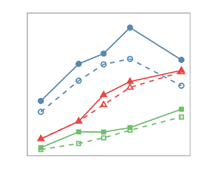
In figure 4 we show the normalised settling velocity enhancement,  $-\langle {u}_z(\boldsymbol {x}^p(t),t)\rangle /u_\eta$, in the 1WC (dashed) and the 2WC (solid) simulation regimes, as a function of $St$, for volume fractions (a) $\varPhi _1$ and (b) $\varPhi _4$, respectively (plots for other volume fractions are shown in the Appendix). Settling enhancements for simulations with $Fr=0.3$, $1$ and $3$ are shown in red, blue and green, respectively. For a given $\varPhi$, we see that the settling enhancement due to turbulence generally increases with (i) increasing $St$, for a given $Fr$, and (ii) decreasing $Fr$, for a fixed $St$, both of which correspond to increasing $Sv$. However, for $Fr=0.3$, a decrease in the settling enhancement is observed when going from $St=1$ to $St=2$ for both the 1WC and 2WC simulations at $\varPhi _1$ and for the 1WC simulations at $\varPhi _3$. For the 1WC case (the explanation for its occurrence in the 2WC case is given below), this reduction can be understood by noting that, for fixed $Fr$, increasing $St$ corresponds to increasing $Sv$, and as discussed at the start of this sub-section, $\langle {u}_z(\boldsymbol {x}^p(t),t)\rangle$ is expected to exhibit a non-monotonic dependence on $Sv$. The values of $St$ and $Fr$ at which $-\langle u_z(\boldsymbol {x}^p(t),t)\rangle / u_{\eta }$ is observed to decrease must therefore correspond to values of $Sv$ that exceed $Sv_{crit}$.

Figure 4. Normalised settling velocity enhancement for the 1WC (dashed) and 2WC (solid) cases for  $\varPhi =1.5\times 10^{-6}$ (a) and $\varPhi =7\times 10^{-5}$ (b), vs $St$. See figure 14 for trends corresponding to other volume fractions.
Figure 5 shows the volume fraction  $\varPhi$ dependence of the normalised settling enhancement for simulations with (a) $Fr=0.3$, and (b) $Fr=3$. Dashed and solid lines denote the results for the 1WC and 2WC simulations, respectively, whereas different line colours denote different $St$. The results show that, even for the smallest volume fraction considered ( $\varPhi _1$), the momentum coupling results in a finite, additional settling enhancement compared with the 1WC case, indicating that the particles are modifying the flow field in measurable ways. As shown in § 4.1, for $\varPhi _1$ the global fluid statistics are almost identical to those of the unladen flow and this is because, for low $\varPhi$, modifications to the flow in the vicinity of the particles make a negligible contribution to the global fluid behaviour. As $\varPhi$ is increased, we observe increasingly large differences between the 1WC and 2WC cases, as expected (note that, physically, the 1WC results should be independent of $\varPhi$; slight variations of the 1WC results when varying $\varPhi$ must therefore be due to statistical convergence effects due to the varying numbers of particles in the flow in each case). In Monchaux & Dejoan (Reference Monchaux and Dejoan2017) it was argued that the enhancement of particle settling speeds in the presence of 2WC compared with the 1WC case occur because, for a 2WC system, the settling inertial particles drag the fluid down with them which reduces the drag force on the particles and enables them to settle faster than in the 1WC case. As $\varPhi$ is increased, this dragging effect on the fluid by the settling particles becomes stronger because of the increased mass loading of the particles, and hence $-\langle u_z(\boldsymbol {x}^p(t),t)\rangle / u_{\eta }$ becomes larger. It was argued in Monchaux & Dejoan (Reference Monchaux and Dejoan2017) that this fluid dragging effect takes over from the preferential sweeping mechanism as being the dominant effect leading to $-\langle u_z(\boldsymbol {x}^p(t),t)\rangle / u_{\eta }>0$. However, in Tom et al. (Reference Tom, Carbone and Bragg2022) it was argued that this is not the case, and that, at least for the parameters they considered, the fluid drag effect actually works together with the preferential sweeping mechanism to further enhance $-\langle u_z(\boldsymbol {x}^p(t),t)\rangle / u_{\eta }$ compared with its value for the 1WC system. This will be investigated further later in this paper.

Figure 5. Normalised settling velocity enhancement vs volume fraction  $\varPhi$, for the 1WC (dashed) and 2WC (solid) cases, for fixed $Fr$: (a) $Fr=0.3$, (b) $Fr=3$. See figure 15 for simulations with $Fr=1$.
The effect of 2WC on  $-\langle u_z(\boldsymbol {x}^p(t),t)\rangle / u_{\eta }$ is seen to become stronger for increasing $St$ (at fixed $Fr$) and/or decreasing $Fr$ (at fixed $St$), i.e. for increasing $Sv$. This occurs because an increase in $Sv$ leads to greater potential energy of the particles, so that there is more energy available to be converted into fluid TKE through the fluid dragging effect, which can lead to an increase for $-\langle u_z(\boldsymbol {x}^p(t),t)\rangle / u_{\eta }$. An implication of this is that, whereas $-\langle u_z(\boldsymbol {x}^p(t),t)\rangle / u_{\eta }$ is expected to exhibit a non-monotonic dependence on $Sv$ in a 1WC system, in the presence of 2WC it may monotonically increase with increasing $Sv$ when $\varPhi$ is sufficiently large for the effects of 2WC to be strong. The data in figure 5 are consistent with this, except for $\varPhi _1$ and $Fr=0.3$, where a decrease of $-\langle u_z(\boldsymbol {x}^p(t),t)\rangle / u_{\eta }$ is observed in going from $St=1$ to $St=2$. However, this is likely because, for $\varPhi _1$, the effects of 2WC are relatively weak and so the non-monotonic dependence of $-\langle u_z(\boldsymbol {x}^p(t),t)\rangle / u_{\eta }$ on $Sv$ that is expected for a 1WC system (and which is also observed in figure 5a) would also be expected for the 2WC case. This also explains the decrease in $-\langle u_z(\boldsymbol {x}^p(t),t)\rangle / u_{\eta }$ observed in figure 4(a) for $\varPhi _1$ and $Fr=0.3$ for the 2WC case when going from $St=1$ to $St=2$, which is not observed for the 2WC at the higher volume fraction $\varPhi _3$ in figure 4(b).
4.3. Preferential sampling:  $St$, $Fr$, $\varPhi$ dependence


Having considered the effect of the parameters  $St, Fr, \varPhi$ on the enhancement of the particle settling velocity, we now turn to consider the mechanism underlying this enhancement. In Monchaux & Dejoan (Reference Monchaux and Dejoan2017), it had been argued that, in the presence of 2WC, the enhanced settling velocities due to turbulence are no longer due to the preferential sweeping mechanism but due to the fluid dragging effect, i.e. the particles drag the fluid down with them which reduces the drag force acting on them leading to enhanced settling speeds. However, in a later study by Tom et al. (Reference Tom, Carbone and Bragg2022), some aspects of this argument were brought into question and the authors shed light on a nuanced perspective. It was shown that the preferential sweeping mechanism still operates in the presence of 2WC, but the particles drag the fluid with them as they are swept down, so that preferential sweeping and the fluid dragging effect act together to enhance the particle settling velocities. We want to explore whether this argument remains true as the parameters are varied, especially when $\varPhi$ is larger.
The preferential sweeping mechanism is associated with the preference for inertial particles to move in downward moving strain-dominated regions of the flow. To explore the role this mechanism plays in governing the settling enhancement, we therefore first consider statistical measures that can quantify the preferential sampling of the flow field. We do this by analysing the PDF  $\mathscr {P}(\mathcal {Q})\equiv \langle \delta (Q^p(t)-\mathcal {Q}\rangle$, where $Q^p(t)\equiv Q(\boldsymbol {x}^p(t),t)$ is the velocity gradient invariant $Q$ measured along the inertial particle trajectory. Figure 6(a) shows $\mathscr {P}(\mathcal {Q})$ (normalised using $\epsilon /(2\nu )$ of the unladen flow) for 1WC (dashed) and 2WC (solid) simulations with $St=1$ particles and with $Fr=0.3$, for all volume fractions $\varPhi$. By convention (see discussion below (4.1a–c)), positive values of $\mathcal {Q}$ correspond to strain-dominated regions whereas negative values correspond to rotation-dominated regions. For small $\varPhi$, the 2WC results are quite similar to the 1WC results, as was also observed in Tom et al. (Reference Tom, Carbone and Bragg2022) for the case $\varPhi _3$ with $Fr=1$. Increasing $\varPhi$ marginally influences the probability of $\mathcal {Q}<0$ regions, which remains consistent with the 1WC trend. This trend parallels the Eulerian PDF of $\mathcal {Q}$ in 2WC shown in figure 1(a). However, as $\varPhi$ is increased, the probability of $\mathcal {Q}>0$ increases significantly, in contrast to the Eulerian PDF of $\mathcal {Q}$ shown in figure 1. This suggests that the increase is likely due to falling particles inducing strain in the flow. Hence, it is important to note that these differences between the 1WC and 2WC results are not only due to differences in the way that the particles are sampling the flow, but also because the statistics of the flow field itself change due to 2WC, as was previously shown in figure 1 for the global statistics of $Q(\boldsymbol {x},t)$.

Figure 6. Results for the Lagrangian PDF  $\mathscr {P}(\mathcal {Q})$ in 1WC and 2WC simulations, along particle trajectories (a) for ${St}_1=1$, $Fr=0.3$ showing $\varPhi$ dependence, and (b) at a constant volume fraction $\varPhi _4=7\times 10^{-5}$, and $Fr=0.3$ showing $St$ dependence. Dashed and solid lines mark the trends for 1WC and 2WC simulations, respectively. The black, solid line corresponds to Eulerian PDF of $\mathcal {P}(\mathcal {Q})$ of the unladen flow. Here, $\mathcal {Q}$ is normalised by $\epsilon /(2\nu )$ from the unladen flow.
In figure 6(b), we show the PDF  $\mathscr {P}(\mathcal {Q})$ at a constant volume fraction $\varPhi _4$, and $Fr=0.3$ for different $St$. Here, solid lines correspond to 2WC simulations, whereas dashed lines correspond to 1WC simulations. For the 1WC simulations, the left tail show a strong $St$ dependence whereas the right tail remains unaffected and traces the unladen fluid limit. This is reminiscent of the observations of Tom et al. (Reference Tom, Carbone and Bragg2022) at $Fr=1$ and volume fraction $\varPhi \approx 1.5 \times 10^{-5}$, and suggests that the expulsion of inertial particles from strongly rotational regions in turbulence is the main mechanism driving preferential concentration. For 2WC simulations at a larger volume fraction $\varPhi _4$, we see that the effects of $St$ on the $\mathcal {Q}<0$ and the $\mathcal {Q}>0$ tails are less and more significant, respectively.
To provide clearer quantitative insight into the degree to which the inertial particles preferentially sample the flow, we can consider the difference between the probability that the particles are in a strain-dominated ( $Q>0$) or a vorticity-dominated ( $Q<0$) region, denoted by $\mathbb {P}(\mathcal {Q}>0)\equiv \int _0^\infty \mathscr {P}(\mathcal {Q})\,{\rm d} \mathcal {Q}$ and $\mathbb {P}(\mathcal {Q}<0)\equiv \int _{-\infty }^0 \mathscr {P}(\mathcal {Q})\,{\rm d} \mathcal {Q}$, respectively. However, even for fluid particles (which sample the flow uniformly), $\mathbb {P}(\mathcal {Q}>0)-\mathbb {P}(\mathcal {Q}<0)\neq 0$, and therefore simply considering $\mathbb {P}(\mathcal {Q}>0)-\mathbb {P}(\mathcal {Q}<0)$ will not provide a direct measure of the degree to which the inertial particles preferentially sample the flow. Therefore, the measure of preferential sampling that we will use is
 \begin{equation} \varphi\equiv\frac{\mathbb{P}(\mathcal{Q}>0)-\mathbb{P}(\mathcal{Q}<0)}{[\mathbb{P}(\mathcal{Q}>0)-\mathbb{P}(\mathcal{Q}<0)]\vert_{St=0}}, \end{equation}
where  $[\mathbb {P}(\mathcal {Q}>0)-\mathbb {P}(\mathcal {Q}<0)]\vert _{St=0}$ denotes $\mathbb {P}(\mathcal {Q}>0)-\mathbb {P}(\mathcal {Q}<0)$ evaluated along the trajectories of fluid particles (and since the flow is incompressible, these single-time statistics are the same as those based on $Q$ measured at fixed locations $\boldsymbol {x}$ in the flow). When $\varphi > 1$, this indicates that the inertial particles exhibit a preference to move in strain-dominated regions of the flow.
In figure 7 we plot  $\varphi$ for different parameter choices. Most strikingly, the results show that the preferential sampling of strain-dominated regions of the flow becomes stronger as $\varPhi$ is increased. This is contrary to expectations based on the argument of Monchaux & Dejoan (Reference Monchaux and Dejoan2017) that 2WC weakens the preferential sampling of the flow and the associated centrifuge mechanism. A potential reason for this difference lies in the interpretation of the joint PDF of $\boldsymbol {S:S}$ and $\boldsymbol {R:R}$ (see § 4.1 for notation) for 2WC simulations with varying volume fraction $\varPhi$ (Monchaux & Dejoan Reference Monchaux and Dejoan2017). This is because, as $\varPhi$ is varied, this PDF is affected both by changes in the particle motion and also changes in the fluid velocity field due to 2WC. As a result, this joint PDF of $\boldsymbol {S:S}$ and $\boldsymbol {R:R}$ measured along the inertial particle trajectories does not give a direct measure of the preferential sampling of the flow by the inertial particles. To test for preferential sampling of the fluid-velocity-gradient field, one must compare the properties of the fluid velocity gradients measured along the inertial particle trajectories with those measured along fluid particle trajectories. In the Appendix, figures 16 and 17 show separately the quantities $\mathbb {P}(\mathcal {Q}>0)-\mathbb {P}(\mathcal {Q}<0)$ and $[\mathbb {P}(\mathcal {Q}>0)-\mathbb {P}(\mathcal {Q}<0)]\vert _{St=0}$, respectively. The results for $\mathbb {P}(\mathcal {Q}>0)-\mathbb {P}(\mathcal {Q}<0)$ show that this quantity reduces as $\varPhi$ is increased, and this is consistent with the results from Monchaux & Dejoan (Reference Monchaux and Dejoan2017) which show that the joint PDF of $\boldsymbol {S:S}$ and $\boldsymbol {R:R}$ measured along the inertial particle trajectories becomes more symmetric about the line $\boldsymbol {S:S}=\boldsymbol {R:R}$ as $\varPhi$ is increased, i.e. that the enhanced probability of being in strain-dominated regions reduces as $\varPhi$ is increased. However, the results also show that $[\mathbb {P}(\mathcal {Q}>0)-\mathbb {P}(\mathcal {Q}<0)]\vert _{St=0}$ decreases as $\varPhi$ is increased, and this is why $\varphi$ increases as $\varPhi$ increases, even though $\mathbb {P}(\mathcal {Q}>0)-\mathbb {P}(\mathcal {Q}<0)$ decreases as $\varPhi$ increases.

Figure 7. Plots of  $\varphi$ (4.2) vs volume fraction $\varPhi$ for simulations with (a) $Fr=0.3$, (b) $Fr=1$ and (c) $Fr=3$. When $\varphi > 1$, this indicates that the inertial particles exhibit a preference to move in strain-dominated regions of the flow.
4.4. Preferential sweeping: $St$, $Fr$, $\varPhi$ dependence


The preferential sweeping mechanism not only argues that inertial particles preferentially sample strain-dominated regions of the flow (which we have just demonstrated is indeed the case), but also that, due to gravity, they will preferentially sample strain-dominated regions of the flow where the vertical fluid velocity points down. Tom et al. (Reference Tom, Carbone and Bragg2022) tested this by computing the quantities
 $$\begin{gather} A \equiv\int_{-\infty}^{0}\langle u_z(\boldsymbol{x}^p(t),t)\rangle_{\mathcal{Q}} \mathscr{P}(\mathcal{Q})\,{\rm d}\mathcal{Q}, \end{gather}$$
 $$\begin{gather}B \equiv\int_{0}^{\infty} \langle u_z(\boldsymbol{x}^p(t),t)\rangle_{\mathcal{Q}}\mathscr{P}(\mathcal{Q})\,{\rm d}\mathcal{Q}. \end{gather}$$
As discussed in Tom et al. (Reference Tom, Carbone and Bragg2022), the preferential sweeping predicts that  $B<0$ and $|B|>|A|$, such that the settling enhancement arises primarily due to contributions from particles in strain-dominated regions of the flow where the fluid velocity is moving downward.
Figure 8(a–c) shows results for  $A$ (blue) and $B$ (red), for 1WC (dashed) and 2WC (solid) cases as a function of $\varPhi$ at $St=1$ and for (a) $Fr=0.3$, (b) $Fr=1$, (c) $Fr=3$. For the 1WC results, $B$ is seen to become more negative as $Fr$ is reduced, indicating that the preferential sweeping becomes stronger as $Sv$ is reduced over the range of $Sv$ considered. The results also show that $A$ is also negative, implying that there is also a contribution to the settling enhancement arising from particles in vorticity-dominated regions of the flow. While this may seem surprising, it was argued in Tom et al. (Reference Tom, Carbone and Bragg2022) that this is not inconsistent with the preferential sweeping mechanism (the reader is referred to that paper for the explanation why). For $Fr=1$ and $Fr=3$, the values of $A$ and $B$ are almost identical for the 1WC and 2WC cases at the lowest $\varPhi$, but for $Fr=0.3$ there is an enhancement in the magnitudes of both $A$ and $B$ due to 2WC even for the lowest $\varPhi$. For each $Fr$, however, both $A$ and $B$ become increasingly negative as $\varPhi$ is increased, while always preserving $|B|>|A|$. As argued in Tom et al. (Reference Tom, Carbone and Bragg2022), this implies that, as $\varPhi$ is increased and 2WC becomes increasingly important, the preferential sweeping mechanism remains active and is the mechanism responsible for the turbulent enhancement of the particle settling speeds. The difference 2WC makes is that, when the particles are swept into downward moving strain-dominated regions of the flow, they are not only swept downwards but also drag the fluid down with them, and this is why $B$ is more negative for the 2WC cases than the 1WC cases at all $St, Fr, \varPhi$ combinations considered.

Figure 8. Plots of  $A$ (4.3), in blue, and $B$ (4.4), in red, for 1WC (dashed) and 2WC (solid) flows for $St=1$ particles as a function of $\varPhi$ with (a) $Fr=0.3$, (b) $Fr=1$ and (c) $Fr=3$. Plots of $A$ (blue) and $B$ (red) at a fixed volume fraction $\varPhi _4=7\times 10^{-5}$ for 1WC (dashed) and 2WC (solid) simulations, with (e) $Fr=0.3$, (f) $Fr=1$, (g) $Fr=3$ showing the $St$ dependence. See figures 18 and 19 for $\varPhi$-, $St$-dependence for other simulations.
Figure 8(d–f) illustrates the  $St$ dependence of $A$ and $B$ at a fixed volume fraction $\varPhi _4=7\times 10^{-5}$ and for (e) $Fr=0.3$, (f) $Fr=1$, (g) $Fr=3$. The results show that the increased negativity of $B$ (as well as $A$) occurs at all $St$ considered. The results also indicate that the difference between the 1WC and 2WC values for $A$ and $B$ becomes larger as $St$ is increased, for a fixed $\varPhi$ and a given $Fr$. This is again because, for a given $Fr$, increasing $St$ corresponds to increased potential energy for the particles, and hence a greater ability to modify the fluid velocity field.
To examine more carefully the relative contributions of both  $A$ and $B$ and their dependence on $\varPhi$, figure 9 shows the ratio $B/A$ for 2WC cases as a function of $\varPhi$ for different $St$ with (a) $Fr=0.3$, (b) $Fr=1$ and (c) $Fr=3$. Large values of $B/A$ indicate cases where preferential sweeping plays a significant role, whereas $B/A=1$ corresponds to the limit where the contributions to $\langle u_z(\boldsymbol {x}^p(t),t)\rangle$ from strain- and rotation-dominated regions are equal, and therefore preferential sweeping plays no role. The results show that the ratio decreases (except for a few cases where it initially increases, but then decreases) with increasing $\varPhi$, showing that the role of preferential sweeping becomes less important as $\varPhi$ increases, in partial agreement with Monchaux & Dejoan (Reference Monchaux and Dejoan2017). However, it is still important for all of the cases; the ratio is greater than 1 even at the largest $\varPhi$, and for many of the cases it is closer to 2 at this $\varPhi$. An interesting and important question is whether preferential sweeping will continue to play an important role as $\varPhi$ is increased even further. The results for $Fr=0.3$ seem to indicate that $B/A$ becomes independent of $\varPhi$ as $\varPhi$ is increased, which could suggest that preferential sweeping remains important even at much larger $\varPhi$. The results for $Fr=1,3$ do not show evidence of a regime where $B/A$ becomes independent of $\varPhi$, but this could be simply because this asymptotic regime occurs at larger $\varPhi$ than we have simulated.


Taken together, these results provide strong evidence that, even in regimes where the mass loading is high enough for the particles to substantially modify the global fluid statistics, the preferential sweeping mechanism remains important for governing how turbulence enhances particle settling speeds. The difference compared with the 1WC case is that, in the 2WC case, the particles are not merely swept around the downward moving side of vortices in the flow but they also (if the mass loading is sufficient) drag the fluid down with them in these regions as they fall. Our results also suggest that preferential sweeping may continue to be important at mass loadings much greater than those considered here, but the evidence is not conclusive.
5. Comparison with previous work
So far, we have considered the impact of 2WC on particle settling and certain flow statistics by comparison with the corresponding results from our DNS for 1WC simulations. We also discussed the ways in which our results compare qualitatively with those of Monchaux & Dejoan (Reference Monchaux and Dejoan2017). In this section we turn to considering a quantitative comparison of our DNS results with selected prior experiments and numerical studies that have parameters closely aligned with the current simulations. This comparison includes the studies by Aliseda et al. (Reference Aliseda, Cartellier, Hainaux and Lasheras2002), Bosse et al. (Reference Bosse, Kleiser and Meiburg2006), Monchaux & Dejoan (Reference Monchaux and Dejoan2017), Berk & Coletti (Reference Berk and Coletti2021) and Hassaini & Coletti (Reference Hassaini and Coletti2022). Table 2 presents a summary of the different simulations and experiments in these studies. It is important to note that, despite their significance, recent works by Petersen et al. (Reference Petersen, Baker and Coletti2019), Rosa et al. (Reference Rosa, Kopeć, Ababaei and Pozorski2022) and Hassaini et al. (Reference Hassaini, Petersen and Coletti2023) were not included in this comparison due to the lack of sufficient parameter overlap. For example, in the study by Petersen et al. (Reference Petersen, Baker and Coletti2019),  $Re_\lambda \geq 300$, in Hassaini et al. (Reference Hassaini, Petersen and Coletti2023), the flow Reynolds number is higher $Re_\lambda \gtrsim 150$ and we have poor overlap in $Fr\sim 0.1, 0.7$ and, in Rosa et al. (Reference Rosa, Kopeć, Ababaei and Pozorski2022), we have poor overlap in the Stokes number $St$ and Rouse number $R=u_\eta Sv/u^\prime$.
Table 2. Details of previous experiments (denoted by E) and numerical simulations (denoted by S). Here,  ${\rm AL}\,{\rm E1}$ and ${\rm AL}\,{\rm E2}$ denote the measurements of Aliseda et al. (Reference Aliseda, Cartellier, Hainaux and Lasheras2002) in isotropic, decaying grid turbulence (squares and circles, respectively, in figure 14(a) of ${\rm AL}$); ${\rm YS}$ indicates the measurements of Yang & Shy (Reference Yang and Shy2005) in stationary, homogeneous, isotropic turbulence generated by a pair of counter-rotating fans (refer to figure 16(a) for data); ${\rm BM}\,{\rm S1}\unicode{x2013}{\rm S3}$ denote the results of DNS from Bosse et al. (Reference Bosse, Kleiser and Meiburg2006) using a stochastic forcing scheme and a computational particle approach (in the Eulerian–Lagrangian framework); see table II ( ${\rm BM}\,{\rm S1}$) and table V, figure 14 (diamond for ${\rm BM}\,{\rm S2}$ and triangle for ${\rm BM}\,{\rm S3}$); ${\rm GW}$ indicates the studies presented in Good et al. (Reference Good, Ireland, Bewley, Bodenschatz, Collins and Warhaft2014): ${\rm GW}\,{\rm E1}$ denotes the experiment of particle settling in soccer-ball apparatus with 32 loudspeaker jets (labelled E1 in ${\rm GW}$ table 1), whereas ${\rm GW}\,{\rm S1}$ marks the results obtained from DNS using a deterministic forcing scheme (simulation labelled S2 in ${\rm GW}$ table 1 interpolated to the same $Fr$ as ${\rm GW}\,{\rm E1}$); see figure 3(a) in ${\rm GW}$ for data; ${\rm MD}$ refers to the numerical studies presented in Monchaux & Dejoan (Reference Monchaux and Dejoan2017) using DNS. The simulations ${\rm S1}$ and ${\rm S2}$ correspond to simulations, for Rouse number $R=\tau _pg/u^\prime =0.25$, with $St=0.36$ and $St=1$, respectively; see table II for additional details; ${\rm BC}\,{\rm E1},2$ indicate the results from the experiments in a turbulence chamber (Berk & Coletti Reference Berk and Coletti2021) with facing jet arrays at two different $Re_\lambda$ (see table 2 and figure 8 in ${\rm BC}$ for data); ${\rm HC}\,{\rm E1},2$ denote the experiments in a similar set-up as ${\rm BC}$, but with the jet arrays activated in a randomised sequence (Hassaini & Coletti Reference Hassaini and Coletti2022); refer to table 1 and figure 3 in ${\rm HC}$ for data.

Figure 10 compares the ratios of the r.m.s. fluid velocities in different directions from our 2WC DNS simulations with data from the DNS of Bosse et al. (Reference Bosse, Kleiser and Meiburg2006) and experiments of Hassaini & Coletti (Reference Hassaini and Coletti2022), hereafter  ${\rm BM}$ and ${\rm HC}$, respectively. See table 2 for the details of these studies. Panel (a) shows the ratio of the horizontal to the vertical r.m.s. velocities, $u^\prime _1/u^\prime _3$ (solid lines) and $u^\prime _2/u^\prime _3$ (dashed lines), as a function of the volume fraction $\varPhi$. The results of ${\rm HC}\,{\rm E1}$ ( ${\rm HC}\,{\rm E2}$) are denoted by black circles (diamonds), and those of ${\rm BM}\,{\rm S1}$ are denoted by black squares. Data from the simulations with parameters closest to ${\rm HC}\,{\rm E1}$ and ${\rm HC}\,{\rm E2}$ are indicated by blue circles and red diamonds, respectively. We see that the r.m.s. velocity in the horizontal direction decreases compared with that in the vertical direction as $\varPhi$ increases. This is because the amount of particle potential energy that is converted to the vertical component of the TKE though the fluid drag mechanism increases with volume fraction $\varPhi$. This observed behaviour is opposite to the trend observed in the experiments of ${\rm HC}$, but in agreement with the DNS results of ${\rm BM}$. Panel (b) shows the ratio of the horizontal r.m.s. velocities for 2WC simulations to that of the corresponding 1WC simulations, $u^\prime _1/u^\prime _{1,\varPhi =0}$ (solid lines) and $u^\prime _2/u^\prime _{2,\varPhi =0}$ (dashed lines), as a function of the volume fraction $\varPhi$. We observe that these ratios decrease as $\varPhi$ increases, which is again in keeping with ${\rm BM}$ but in contrast to ${\rm HC}$.

Figure 10. Ratio of the (a) horizontal to vertical turbulence intensities  $u^\prime _1/u^\prime _3$, $u^\prime _2/u^\prime _3$ and (b) horizontal turbulence intensities for 2WC in unladen simulations $u^\prime _1/u^\prime _{1,\varPhi =0}$, $u^\prime _2/u^\prime _{2,\varPhi =0}$ for DNS (coloured symbols) and data from previous work (in black). Experimental results from Hassaini & Coletti (Reference Hassaini and Coletti2022) figure 3(a) are shown in black circles ( $St=0.3$) and black diamonds ( $St=2.6$), denoted by ${\rm HC}\,{\rm E1}$ and ${\rm HC}\,{\rm E2}$, respectively. Results from Bosse et al. (Reference Bosse, Kleiser and Meiburg2006) table II, denoted by ${\rm BM}\,{\rm S1}$, are given by black squares. Solid and dashed lines for the current and previous numerical results simply correspond to data along to two different horizontal directions. Details of the previous works are given in table 2.
A plausible explanation for the discrepancy between the DNS (both ours and  ${\rm BM}$) and the experimental results of ${\rm HC}$ is that the particles introduce a certain level of anisotropy into the flow in the measurement area of the experiments which is not present in the DNS. In particular, since inertial particles carry a memory of their interaction with the flow (Bragg & Collins Reference Bragg and Collins2014a,Reference Bragg and Collinsb), they may carry into the measurement area a memory of their interaction with the large-scale flow which is anisotropic in the experiment even in the absence of the particles due to the jets used by ${\rm HC}$ to force the flow. This would then cause the particles to transfer momentum to the flow in the measurement region in an anisotropic manner, even though the measurement region is small enough such that in the absence of the particles the flow would be approximately locally isotropic. By contrast, our DNS and that of ${\rm BM}$ force the large scales of the flow in an isotropic manner, and all anisotropy in the flow emerges solely due to the particle settling.
In our DNS, TKE dissipated at the small scales is re-injected into the flow at the large scales in an isotropic manner. This means that, for the subset of Fourier modes that are forced, the flow anisotropy that would otherwise arise for these Fourier modes is effectively suppressed. However, this is not likely to be the cause of the discrepancy between the DNS and experiments noted above for the following reason: in the absence of forcing, some of the vertical kinetic energy injected to the flow due to the particle settling would be transferred to the horizontal fluid motions due to the pressure-strain redistribution effect. If anything, our isotropic forcing would artificially enhance this redistribution of energy from the vertical to horizontal flow motions, and therefore cause the ratios  $u^\prime _1/u^\prime _3$ and $u^\prime _2/u^\prime _3$ to be artificially enhanced by the isotropic forcing, not reduced.
Figure 11 compares the TKE dissipation rate (normalised by 1WC values) of  ${\rm BM}\,{\rm S1}$ (black), which corresponds to $St=1$ and $Fr=1$, with the corresponding values from the current 2WC DNS (red) with the closest parameters. In contrast to ${\rm BM}\,{\rm S1}$, which predicts an initial decrease of $\epsilon$ with $\varPhi$ before increasing again, the current simulations predict a monotonic increase in the dissipation rate. One possible reason for this difference is due to differences in the Reynolds numbers of the flow, since ours has $Re_\lambda \approx 88$ while that of ${\rm BM}\,{\rm S1}$ has a much lower value of $Re_\lambda \approx 42$. Indeed, figure 3 shows that, for some choices of $St,Fr$, $\epsilon$ is also observed to vary non-monotonically with $\varPhi$ in our DNS, and variations in $Re_\lambda$ as well as $St,Fr$ may also lead to similar regimes. Another possible explanation is due to the different forcing methods used in the DNS (discussed more at the end of this section), with our DNS using a deterministic forcing that maintains a constant flow TKE, while Bosse et al. (Reference Bosse, Kleiser and Meiburg2006) use a stochastic method that injects a statistically constant amount of energy into the flow. An alternate cause of these disparities could be the different interpolation schemes used to compute the Stokes drag and the particle-momentum feedback (2.4a,b); Bosse et al. (Reference Bosse, Kleiser and Meiburg2006) implemented a tri-linear interpolation method whereas our study utilised a seventh-order B-spline interpolation. Exactly how these different methods would impact the results in figure 11 is not obvious, however.

Figure 11. Comparison of the TKE dissipation rate (normalised by 1WC values) for the current simulations (red circles) and Bosse et al. (Reference Bosse, Kleiser and Meiburg2006) table II (black diamonds), denoted by  ${\rm BM}\,{\rm S1}$, vs volume fraction $\varPhi$.
Figure 12 compares the normalised Lagrangian PDF  $\mathscr {P}(\mathcal {Q})$ for the current simulations with experimental results of Berk & Coletti (Reference Berk and Coletti2021). Note that the $\mathcal {Q}$ defined here is the negative of that used in ${\rm BC}$, and that the PDFs have been normalised by their standard deviation to facilitate the comparison. The black solid and dashed lines show, for reference, the Eulerian PDFs from the 1WC (or unladen) simulations and the experiment ${\rm BC}$, respectively. Black circles and diamonds correspond to measurements along Lagrangian particle trajectories in ${\rm BC}\,{\rm E1}$ ( $St=1.2$) and ${\rm BC}\,{\rm E2}$ ( $St=2.1$), respectively, for $\varPhi \approx 10^{-7}$; details of these experiments are given in table 2. The results from our 1WC and 2WC simulations with parameters closest to the experiments are shown by the (dashed for 1WC and solid for 2WC) yellow ( $St=1$) and purple ( $St=2$) lines, respectively. It is noteworthy that the Eulerian PDF from ${\rm BC}$ is quite close to the 1WC (effectively unladen) DNS results for the left tail (corresponding to rotation-dominated regions) but predicts a much larger probability of straining events (see the heavier right tail), compared with the DNS. One possible explanation for this significant disagreement is that the difference arises due to the $Re_\lambda$ of the DNS being much lower ( $Re_\lambda \approx 88$) than that in the experiments ( $Re_\lambda \geq 280$). However, this does not seem likely because it is known that the vorticity field is more intermittent than the strain-rate field (Tsinober Reference Tsinober2001), and so the effect of $Re_\lambda$ on the left tail of the PDF should be stronger than that on the right tail, yet the DNS and experiments agree well for the left tail. A more plausible explanation for the difference is that it results from large-scale shear in the experiments due to the jets, which may have a significant effect on the velocity-gradient field during extreme events in the flow where large- and small-scale motions can exhibit significant coupling.

Figure 12. Comparison of the current DNS results for normalised Lagrangian PDFs  $\mathscr {P}(\mathcal {Q})$ (symbols) in 1WC and 2WC simulations and the experiments of Berk & Coletti (Reference Berk and Coletti2021), hereafter ${\rm BC}$. Black solid line corresponding to the 1WC simulations, which is the same as for the unladen flow, and the black dashed line corresponds to the red line from figure 8 of ${\rm BC}$ (corresponding to the unladen fluid statistics), are shown for reference. Black circles and diamonds correspond to measurements along Lagrangian particle trajectories in ${\rm BC}\,{\rm E1}$ and ${\rm BC}\,{\rm E2}$, respectively, for $\varPhi \approx 10^{-7}$. See table 2 for the details of these experiments. Here, $\sigma _{\mathcal {Q}}$ denotes the standard deviation of $Q$.
$Q$.
In figure 13 we present a comparison of our 1WC and 2WC DNS results for the particle settling velocity enhancement with previous results, both experimental and numerical. Dashed and solid lines represent the current DNS results with 1WC and 2WC, respectively, whereas dotted lines and open symbols (no lines) represent previous experimental and numerical results, respectively. Table 2 summarises the notation for these experiments and simulations. Plots at a fixed volume fraction  $\varPhi \approx 10^{-6}$, vs $St$, are shown in figure 13(a) for $Fr \approx 0.3$. The current 2WC results (solid green line) agree well with the experimental results (red dotted line) of ${\rm GW}\,{\rm E1}$ for $St \leq 0.7$, while over-predicting the settling enhancement for $St\geq 1$ by 30 %–50 %. In this parameter range, we see that the 1WC DNS result is actually in better agreement with the experimental data. It is worth pointing out that the current 1WC DNS results differ in significant ways from those of Good et al. (Reference Good, Ireland, Bewley, Bodenschatz, Collins and Warhaft2014) in blue ( ${\rm GW}\,{\rm S1}$), even though they are generated using essentially the same DNS code based on Ireland et al. (Reference Ireland, Vaithianathan, Sukheswalla, Ray and Collins2013). In Tom et al. (Reference Tom, Carbone and Bragg2022) it was discussed that very long time averages (such as we use in our DNS) are needed for the particle settling velocity enhancement results to converge, and that the time averaging window used in Good et al. (Reference Good, Ireland, Bewley, Bodenschatz, Collins and Warhaft2014) was relatively short. This is most likely the explanation for the difference in the results, and highlights the importance of ensuring statistical convergence of the particle settling velocities.

Figure 13. Comparison of 1WC (dashed lines) and 2WC (solid lines) DNS results for settling velocity enhancement (normalised by  $u^{\prime }$), as a function of (a,b) $St$ for different $\varPhi$ and $Fr$, (c) $\varPhi$ for a constant $St$ and $Fr$, with previous studies. See table 2 for details of experiments and numerical simulations. Experimental and numerical results from previous studies are shown by dotted lines and open symbols, respectively.
In figure 13(b), the dashed and the solid green lines show the settling enhancement vs  $St$, for the current 1WC and 2WC simulations (at $\varPhi _3=1.5\times 10^{-5}$ and $Fr_2=1$), respectively. The dotted green line denotes the results from experiment ${\rm AL}\,{\rm E1}$ (see table 2). The black diamond marks the corresponding prediction of ${\rm BM}\,{\rm S2}$. Our 2WC results align well with the measured settling velocity enhancement for $St \geq 0.7$; however, the agreement is quantitatively poor for smaller $St$. Figure 13(b) also compares the settling velocity enhancement predictions from our current simulations with those from previous experiments at volume fraction $\varPhi =7\times 10^{-5}$. The dotted and the solid yellow lines correspond, respectively, to the experiment ${\rm AL}\,{\rm E2}$ and the current 2WC DNS at $\varPhi _4$ and $Fr_2$. Note that both the experiments by ${\rm AL}$ correspond to $Fr \approx 1.6$, whereas the numerical simulations are for $Fr=1$, and the impact of this difference is not known. The corresponding data for the 1WC simulation and the data from ${\rm BM}\,{\rm S3}$ are given by the dashed green line (1WC trend for $\varPhi _4$ is the same as $\varPhi _3$ and hence not shown separately) and the black star, respectively. Compared with ${\rm BM}\,{\rm S3}$, the current results are in better agreement with the experimental data, however, the estimated settling enhancements are consistently smaller than the measured values for $St<2$. In particular, the predicted settling enhancement is approximately three times smaller than the observed values for the $St=0.3$. Yang & Shy (Reference Yang and Shy2005), hereafter ${\rm YS}$, and ${\rm BM}$ discuss, in detail, the shortcomings of the set-up in ${\rm AL}$, which potentially explain the larger values of the settling enhancement in ${\rm AL}\,{\rm E1},2$. However, it is unclear why the largest discrepancies are observed for small $St$; disagreement with our data is only approximately $20\,\%$ for $St \approx 1$.
In figure 13(b), the dashed, solid and the dotted brown lines show the results for the settling enhancement, vs  $St$, for the current 1WC and 2WC DNS simulations (at $\varPhi _4$, $Fr_1$) and the results of ${\rm YS}$ figure 16, respectively. Our 2WC results for this quantity are much larger than those of ${\rm YS}$; ${\rm BM}$ also have DNS results for similar parameters (not shown here) and their results also disagreed considerably with the corresponding results of ${\rm YS}$. Figure 13(c) compares the $\varPhi$ dependence of the settling velocity enhancement results from the current 1WC (dashed lines) and 2WC (solid lines) simulations with those from ${\rm BM}$ (black square) and ${\rm MD}$. Refer to Monchaux & Dejoan (Reference Monchaux and Dejoan2017, table II) for the details of the simulations ${\rm MD}\,{\rm S1}$ and ${\rm MD}\,{\rm S2}$. The numerical simulations ${\rm S1}$ and ${\rm S2}$ from ${\rm MD}$ correspond to $St=0.36$ (orange circle) and $St=1$ (red square), at a constant Rouse number $R=\tau _pg/u^\prime =0.25$; see solid black line with downward triangle and solid blue line with circle in ${\rm MD}$ figure 3(b) for the data. For the parameter choices of our DNS results shown, the Rouse number is $R \simeq 0.29$. Overall we see quite good agreement of the current 2WC DNS results with ${\rm BM}\,{\rm S1}$, ${\rm MD}\,{\rm S1}$ and ${\rm MD}\,{\rm S2}$.
Summing up the results presented in this section, we find good qualitative agreement and generally reasonable quantitative agreement among the DNS results that have been considered. The parameters in the different DNS studies are not exactly the same (we compared those with the closest parametric overlap), and therefore exact quantitative agreement is not expected. Other than differences in the parameters, the DNS differ in how the momentum coupling term is implemented numerically as well as how the flow is forced. The particle-momentum feedback on the computational grid in the current work follows that from Carbone et al. (Reference Carbone, Bragg and Iovieno2019) and Tom et al. (Reference Tom, Carbone and Bragg2022). On the other hand, Bosse et al. (Reference Bosse, Kleiser and Meiburg2006) and Monchaux & Dejoan (Reference Monchaux and Dejoan2017) implement a tri-linear interpolation method and the particle-in-cell method, respectively, for the momentum feedback term. The forcing scheme we use follows that from Tom et al. (Reference Tom, Carbone and Bragg2022) and the work of Good et al. (Reference Good, Ireland, Bewley, Bodenschatz, Collins and Warhaft2014). Monchaux & Dejoan (Reference Monchaux and Dejoan2017) also use a forcing scheme whereby the dissipated energy is reintroduced back into the system. Instead of maintaining a constant TKE, Bosse et al. (Reference Bosse, Kleiser and Meiburg2006) used a forcing method that maintains a constant TKE injection rate following Eswaran & Pope (Reference Eswaran and Pope1988). It should be noted that the classical argument that the energy dissipation and particle dynamics are mainly governed by the small-scale dynamics does not apply, since the turbulent statistics change according to how the large-scale forcing is implemented. To determine the influence of these different numerical methodologies on the results for particle settling, the research community would benefit greatly from a future study where results from different DNS using identical parameters are compared, similar to what was done in Marchioli et al. (Reference Marchioli, Soldati, Kuerten, Arcen, Tanière, Goldensoph, Squires, Cargnelutti and Portela2008) to compare different DNS codes for inertial particle transport in wall-bounded turbulence. Comparisons of DNS with experimental results showed that, for some quantities, the DNS and experiments show good qualitative agreement but quite poor quantitative agreement, while for other quantities they even differ quantitatively. However, for the particle settling enhancement results, different experiments gave very different results. It is not clear whether these differences occur due to physical differences in the experiments (different parameters, flow types etc.) or due to limitations in the measurement and/or data post-processing methodologies. Therefore, just as it is important in future work for the results from different DNS codes to be carefully compared in order to understand their differences, so also there needs to be a concentrated effort to understand differences between published experimental results. Only when this has been done will it be possible to make progress on understanding exactly which modelling approximations made in the DNS are principally responsible for the discrepancies between the DNS and experimental results.
6. Conclusions
We have conducted 1WC and 2WC DNS of settling, sub-Kolmogorov scale, heavy, inertial particles in homogeneous turbulence over a wide range of Froude numbers  $Fr$, Stokes numbers $St$ and volume fractions $\varPhi$ (the particle density was held constant, so that the mass loading $\varPhi _m$ is proportional to $\varPhi$). For each combination of $St, Fr$, five different values of $\varPhi$ were considered that span two orders of magnitude. We first considered the impact of 2WC on various global fluid statistics, including the properties of the strain-rate and vorticity fields and TKE dissipation rates, as well as the energy spectrum to consider the impact of 2WC on different scales in the flow. At the smallest $\varPhi$, the PDF of $Q$ (the second invariant of the velocity gradient tensor) retains the characteristic skewness that is seen for the unladen flow which is associated with the vorticity field being more intermittent than the strain-rate field. However, the PDF becomes increasingly symmetric as $\varPhi$ is increased, indicating that the momentum feedback from the particles amplifies regions of high strain rate. This effect of 2WC depends much more strongly on $Fr$ than on $St$ for the parameter regimes considered. For the energy spectrum we observe that, as $\varPhi$ is increased, there is an accumulation of energy in the high-wavenumber modes, which also corresponds to an increase in the TKE dissipation rate. Moreover, as $\varPhi$ is increased, the fraction of TKE associated with the vertical velocity fluctuations also increases, and this is due to the conversion of particle potential energy to the vertical component of TKE through the effect of the particles dragging the surrounding fluid down with them as they settle, and thereby doing work on the surrounding flow. This observation contrasts with experimental results which have shown an increase in the horizontal turbulence intensity. Possible explanations for this difference were discussed.
We then turned to considering how the settling velocity of the particles depends on  $St, Fr$ and $\varPhi$. We find that, even for the smallest $\varPhi$ considered ( $\varPhi =1.5\times 10^{-6}$, corresponding to a mass loading of $7.5\times 10^{-3}$), the mean settling speed of the particles can be appreciably larger for the 2WC case than the 1WC case for some choices of $St$ and $Fr$. For both 1WC flows and 2WC flows at low $\varPhi$, the largest enhancement of the mean settling velocity compared with the Stokes settling velocity occurs for $St=1$ and $Fr=0.3$, and the enhancement exhibits a non-monotonic dependence on $Sv$ which is expected since the settling enhancement must go to zero in the two limits $Sv \to \infty$ and $Sv \to 0$. However, for 2WC flows with higher $\varPhi$ this non-monotonic dependence does not occur since as $Sv$ is increased, the particles are increasingly effective in dragging the fluid down with them which reduces the drag force on the particle and enhances their settling velocity. Due to this, the difference between the particle settling speeds in the 1WC and 2WC flows increases with increasing $Sv$. In contrast to our DNS results, previous experimental results observed a non-monotonic dependence of the settling enhancement on $Sv$ when considering volume fractions up to $7\times 10^{-5}$.
The next step was to understand how the mechanisms governing the enhanced particle settling depends on  $\varPhi$. In particular, we wanted to understand whether preferential sweeping remains relevant in 2WC flows when $\varPhi$ becomes large enough for the global fluid statistics to be strongly affected by the particles. The preferential sweeping mechanism is based on the argument that the following two things should occur: (i) the particles should preferentially sample strain-dominated regions of the flow (which they would do even in the absence of gravity), and (ii) the particles should preferentially sample strain-dominated regions where the vertical fluid velocity points down (which they would not do in the absence of gravity, if the flow is isotropic). To test the first part, we computed the PDF of $Q$ measured along the trajectories of the settling inertial particles and compared them with results based on $Q$ measured along fluid particle trajectories. The Lagrangian PDF of $Q$ shows that, in the vicinity of inertial particles, the flow is more likely to be strain dominated as the volume fraction increases. We also compared the probability of particles being in $Q>0$ regions compared with $Q<0$ regions, normalised by the corresponding probability for fluid particles. The results showed that, not only is preferential sampling still active in the 2WC flows, but that it actually becomes stronger as $\varPhi$ is increased. To test the second part, we computed the settling velocity enhancement conditioned on the particles being in $Q>0$ or $Q<0$ regions. The results showed that, at all $St$,
$St$,  $Fr$ and $\varPhi$ combinations considered, the strongest contribution to the enhanced particle settling velocities comes from particles in strain-dominated regions of the flow, consistent with the preferential sweeping mechanism. The results indicate that the imbalance in the contribution from $Q>0$ and $Q<0$ regions reduces as $\varPhi$ is increased, for a given $St\ {\rm and}\ Fr$. However, the imbalance does not vanish and remains significant at the highest $\varPhi$ considered. The results also indicate that, at least for low $Fr$, the dominance of the contribution from strain-dominated regions might persist to higher $\varPhi$ than we have considered.
Our results therefore support the idea that preferential sweeping remains active in governing the enhanced settling velocity of inertial particles in turbulent flows with 2WC, even though it was originally presented as a mechanism in the context of 1WC flows by Maxey (Reference Maxey1987). This was demonstrated in Tom et al. (Reference Tom, Carbone and Bragg2022) for low values of  $\varPhi$, where the global fluid statistics are weakly affected by the particles, and only the flow in the vicinity of the particles is strongly affected. We have now demonstrated that this conclusion also holds in 2WC flows where $\varPhi$ is large enough for the particles to significantly affect the global fluid statistics. The primary distinction compared with the 1WC limit lies in the fact that, in the 2WC limit, the particles intensify the downward flow of the fluid due to the drag force they exert on the flow. This augmentation leads to an increase in the local fluid velocity and, consequently, higher settling rates in areas where particle clustering occurs. These regions tend to be dominated by strain, as preferential concentration remains in effect, resulting in preferential sweeping and subsequent settling enhancement.
In our DNS, a relatively small Taylor Reynolds number  $Re_\lambda =O(10^2)$ was considered, a restriction imposed due to the computational expense of exploring a significant portion of the $St, Fr, \varPhi$ parameter space. It is important in future work to consider 2WC flows with much larger $Re_\lambda$, where there is a large range of scales in the flow. The results could then be analysed from the perspective of the multiscale preferential sweeping mechanism that was presented in Tom & Bragg (Reference Tom and Bragg2019), which would provide a way to understand how flow scales of different sizes contribute to the enhanced settling velocity of inertial particles in turbulent flows. Such an attempt was done in Tom et al. (Reference Tom, Carbone and Bragg2022), however, that study also used $Re_\lambda =O(10^2)$ and so the range of scales in the flow was quite small. New DNS of 2WC flows with high $Re_\lambda$ would provide insight into how 2WC modifies the sweeping contribution from different scales in the flow which is important for atmospheric contexts, for example, where typically $Re_\lambda \geq O(10^4)$.
In the final section of the paper we compared results from our DNS with other DNS studies as well as experiments. Overall, good qualitative agreement in results for the turbulence anisotropy, TKE dissipation rates, settling velocity enhancements and Lagrangian PDFs was observed between the different DNS studies. Quantitative differences could be due to the fact that the parameters in the DNS were not exactly the same, and also differences in the numerical implementation of the particle-momentum feedback term and the forcing method used to generate a statistically stationary flow. Discrepancies between the DNS results and experiments were observed, but discrepancies were also observed between experiments. Hence, it is essential in future work for the research community to seek to understand the cause of the variations among different DNS results, as well as among different experimental results, since only then will it be possible to meaningfully investigate the cause of the discrepancies between the DNS and experiments, and identify the particular modelling approximations in the DNS that must be improved.
Acknowledgements
S.B. gratefully acknowledges S.L. Rani for their invaluable feedback and the insightful discussion on numerical techniques.
Funding
This work was supported by the National Aeronautics and Space Administration Weather and Atmospheric Dynamics program (grant no. NASA 80NSSC20K0912). The computational resources used were provided by the Extreme Science and Engineering Discovery Environment (XSEDE) under allocation CTS170009, which is supported by National Science Foundation (NSF) grant no. ACI-1548562 (Towns et al. Reference Towns2014). Specifically, the Stampede2 cluster operated by Texas Advanced Computing Center (TACC) and the Expanse cluster operated by San Diego Supercomputer Center (SDSC) were used to obtain the results in this work. The Duke Computing Cluster (DCC) operated by Duke University Research Computing was also used to obtain some of the preliminary results for this study.
Declaration of interests
The authors report no conflict of interest.
Appendix
Table 3. Flow parameters in DNS of 2WC simulations for different volume fraction Φ, Stokes number St and Froude number Fr. The Stokes number and Froude number are defined with respect to the unladen DNS statistics.


Figure 14. Normalised settling velocity enhancement for the 1WC (dashed) and 2WC (solid) cases for (a)  $\varPhi _2=7\times 10^{-6}$, (b) $\varPhi _3=1.5\times 10^{-5}$ and (c) $\varPhi _5=1.5\times 10^{-4}$, vs $St$. Figure 4 in the text shows the results for other volume fractions.

Figure 15. Normalised settling velocity enhancement vs volume fraction  $\varPhi$, for the 1WC (dashed) and 2WC (solid) cases for $Fr=1$. Figure 5 in the text shows the results for $Fr=0.3$ and $Fr=3$.

Figure 16. Plots showing  $\mathbb {P}(\mathcal {Q}>0)-\mathbb {P}(\mathcal {Q}<0)$ vs volume fraction $\varPhi$ for particles with different Stokes number $St$, for simulations with (a) $Fr=0.3$, (b) $Fr=1$ and (c) $Fr=3$. The corresponding values for the 1WC simulations are also shown for reference.

Figure 17. Plots showing  $[\mathbb {P}(\mathcal {Q}>0)-\mathbb {P}(\mathcal {Q}<0)]\vert _{St=0}$ vs volume fraction $\varPhi$ for simulations with (a) $Fr=0.3$, (b) $Fr=1$ and (c) $Fr=3$. The corresponding values for the 1WC simulations are also shown for reference.

Figure 18. Plots of  $A$ (blue) and $B$ (red) vs volume fraction $\varPhi$, for 1WC (dashed) and 2WC (solid) flows for particles with (a–c) ${St}_1=0.3$, (d–f) ${St}_2=0.5$, (g–i) ${St}_3=0.7$ and (j–l) ${St}_5=2$. Panels (a,d,g,j) correspond to simulations with $Fr=0.3$; panels (b,e,h,k) correspond to simulations with $Fr=1$; panels (c,f,i,l) correspond to simulations with $Fr=3$. See figure 8 for the volume fraction dependence in simulations with ${St}_4$ particles.

Figure 19. Plots of  $A$ (blue) and $B$ (red) vs Stokes number $St$, for 1WC (dashed) and 2WC (solid) flows for volume fractions (a–c) $\varPhi _1$, (d–f) for $\varPhi _2$, (g–i) $\varPhi _3$ and (j–l) $\varPhi _5$. Panels (a,d,g,j) correspond to simulations with $Fr=0.3$; panels (b,e,h,k) correspond to simulations with $Fr=1$; and panels (c,f,i,l) correspond to simulations with $Fr=3$. See figure 8 for the $St$-dependence in simulations with volume fraction $\varPhi _4$.


 Open access