


1. Introduction
The theory of iteration of transcendental entire functions $f \colon \mathbb{C} \rightarrow \mathbb{C}$
dates back to Fatou’s seminal work from 1926; [
Reference Fatou11
]. The locus of stable behaviour of such a function – more precisely, the set of
$f \colon \mathbb{C} \rightarrow \mathbb{C}$
dates back to Fatou’s seminal work from 1926; [
Reference Fatou11
]. The locus of stable behaviour of such a function – more precisely, the set of $z\in \mathbb{C}$
at which the family
$z\in \mathbb{C}$
at which the family $\{f^n\}_{n\in\mathbb{N}}$
is equicontinuous with respect to the spherical metric – is today called the Fatou set F(f), while its complement
$\{f^n\}_{n\in\mathbb{N}}$
is equicontinuous with respect to the spherical metric – is today called the Fatou set F(f), while its complement $J(\,f)\;:\!=\; \mathbb{C} \setminus F(\,f)$
is the Julia set. We are also interested in the escaping set
$J(\,f)\;:\!=\; \mathbb{C} \setminus F(\,f)$
is the Julia set. We are also interested in the escaping set
 \begin{equation*}I(\,f)\;:\!=\; \{z\in \mathbb{C} \colon f^n(z)\to \infty \text{ as } n\to \infty\},\end{equation*}
as $J(\,f)=\partial I(\,f)$
and, in the cases we will consider,
$J(\,f)=\partial I(\,f)$
and, in the cases we will consider, $J(\,f)=\overline{I(\,f)}$
; [
Reference Erëmenko and Lyubich9
].
$J(\,f)=\overline{I(\,f)}$
; [
Reference Erëmenko and Lyubich9
].
Fatou observed that the Julia sets of certain sine functions contain infinitely many curves to infinity. In the 1980s, Devaney, with a number of co-authors, studied this phenomenon further, showing the existence of such curves for some functions in the exponential family $E_\kappa \colon z \mapsto e^z+ \kappa$
,
$E_\kappa \colon z \mapsto e^z+ \kappa$
, $\kappa \in \mathbb{C} \setminus \{0\}$
. These curves, that escape uniformly to infinity, are now known as (Devaney) hairs or dynamic rays, and they provide a foliation of the escaping set
$\kappa \in \mathbb{C} \setminus \{0\}$
. These curves, that escape uniformly to infinity, are now known as (Devaney) hairs or dynamic rays, and they provide a foliation of the escaping set $I(E_\kappa)$
for all
$I(E_\kappa)$
for all $\kappa$
; [
Reference Schleicher and Zimmer31
]. See the formal definition of dynamic ray in Definition 4·3.
$\kappa$
; [
Reference Schleicher and Zimmer31
]. See the formal definition of dynamic ray in Definition 4·3.
If the asymptotic value of $E_\kappa$
, i.e., its parameter
$E_\kappa$
, i.e., its parameter $\kappa$
, converges to an attracting or parabolic cycle, then all dynamic rays of
$\kappa$
, converges to an attracting or parabolic cycle, then all dynamic rays of $E_\kappa$
land, that is, have a unique finite accumulation point; [
Reference Rempe22
]. This provides a total description of
$E_\kappa$
land, that is, have a unique finite accumulation point; [
Reference Rempe22
]. This provides a total description of $J(E_\kappa)$
as a collection of unbounded escaping curves together with their landing points; compare to [
Reference Aarts and Oversteegen1
,
Reference Alhamed3
] for further topological characterisations. However, there is no such complete description of
$J(E_\kappa)$
as a collection of unbounded escaping curves together with their landing points; compare to [
Reference Aarts and Oversteegen1
,
Reference Alhamed3
] for further topological characterisations. However, there is no such complete description of $J(E_\kappa)$
when
$J(E_\kappa)$
when $\kappa$
escapes to infinity. In contrast, Rempe showed in [
Reference Rempe23
] that for escaping parameters, the accumulation sets of uncountably many dynamic rays of
$\kappa$
escapes to infinity. In contrast, Rempe showed in [
Reference Rempe23
] that for escaping parameters, the accumulation sets of uncountably many dynamic rays of $E_\kappa$
are indecomposable continua containing the rays themselves.
$E_\kappa$
are indecomposable continua containing the rays themselves.
The existence of dynamic rays is now known for a much larger class of functions belonging to the Eremenko–Lyubich class $\mathcal{B}$
, which consists of all transcendental entire functions with bounded singular set. Recall that for an entire map f, its singular set S(f) is the closure of the set of its asymptotic and critical values. More precisely, it is shown in [
Reference Rottenfusser, Rückert, Rempe and Schleicher27
] that for certain
$\mathcal{B}$
, which consists of all transcendental entire functions with bounded singular set. Recall that for an entire map f, its singular set S(f) is the closure of the set of its asymptotic and critical values. More precisely, it is shown in [
Reference Rottenfusser, Rückert, Rempe and Schleicher27
] that for certain $f\in \mathcal{B}$
, including all those of finite order, some iterate of every
$f\in \mathcal{B}$
, including all those of finite order, some iterate of every $z\in I(\,f)$
can be connected to infinity by a dynamic ray. As in the exponential case, the landing behaviour of rays for such an f depends on the behaviour under iteration of their singular set, that is, on their postsingular set
$z\in I(\,f)$
can be connected to infinity by a dynamic ray. As in the exponential case, the landing behaviour of rays for such an f depends on the behaviour under iteration of their singular set, that is, on their postsingular set $P(\,f)\;:\!=\; \overline{\bigcup^\infty_{n=0} f^n(S(\,f))}$
. Note that for f a postsingularly bounded entire function, P(f) is nicely separated from infinity, where dynamic rays start. This has played a crucial role when proving that all dynamic rays of certain
$P(\,f)\;:\!=\; \overline{\bigcup^\infty_{n=0} f^n(S(\,f))}$
. Note that for f a postsingularly bounded entire function, P(f) is nicely separated from infinity, where dynamic rays start. This has played a crucial role when proving that all dynamic rays of certain $f \in \mathcal{B}$
with bounded postsingular set land, e.g., [
Reference Alhamed, Rempe and Sixsmith4
,
Reference Mihaljević–Brandt15
,
Reference Rempe24
,
Reference Schleicher30
].
$f \in \mathcal{B}$
with bounded postsingular set land, e.g., [
Reference Alhamed, Rempe and Sixsmith4
,
Reference Mihaljević–Brandt15
,
Reference Rempe24
,
Reference Schleicher30
].
In this paper we are interested in the case when critical values escape. Note that the singular set of any map in the cosine family, that is, of the form
 \begin{equation*}C_{a,\,b} \colon z\longmapsto ae^z+be^{-z} \quad \text{ for }a,\,b\in \mathbb{C}\setminus \{0\},\end{equation*}
consists of two critical values, with their preimages being critical points of local degree 2. The explicit nature of this family will allow us to obtain a complete description of the Julia set of certain cosine maps with escaping critical values. But first, we note that, as in the exponential case, when both critical values of $C_{a,\,b}$
belong to an attracting basin all dynamic rays land [
Reference Rottenfusser, Rückert, Rempe and Schleicher27
], and the same holds when
$C_{a,\,b}$
belong to an attracting basin all dynamic rays land [
Reference Rottenfusser, Rückert, Rempe and Schleicher27
], and the same holds when $P(C_{a,\,b})$
is strictly preperiodic [
Reference Schleicher29
].
$P(C_{a,\,b})$
is strictly preperiodic [
Reference Schleicher29
].
If, instead, a critical value of $C_{a,\,b}$
escapes to infinity, dynamic rays split at critical points, and the structure of
$C_{a,\,b}$
escapes to infinity, dynamic rays split at critical points, and the structure of $J(C_{a,\,b})$
is much more complicated. To illustrate this, consider the map
$J(C_{a,\,b})$
is much more complicated. To illustrate this, consider the map $ C_{1/2,1/2} \colon z\mapsto \cosh(z)$
, whose critical values
$ C_{1/2,1/2} \colon z\mapsto \cosh(z)$
, whose critical values $-1$
and 1 escape to infinity in
$-1$
and 1 escape to infinity in $\mathbb{R}^+$
. Note that 0 is a critical point, and it is easy to check that
$\mathbb{R}^+$
. Note that 0 is a critical point, and it is easy to check that $(-\infty, 0]$
and
$(-\infty, 0]$
and $[0, \infty)$
are pieces of dynamic rays. The vertical segments
$[0, \infty)$
are pieces of dynamic rays. The vertical segments $[0, -i\pi /2]$
and
$[0, -i\pi /2]$
and $[0, i\pi /2]$
are mapped univalently to
$[0, i\pi /2]$
are mapped univalently to $[0, 1] \subset \mathbb{R}^+$
, and thus, the union of each segment with either
$[0, 1] \subset \mathbb{R}^+$
, and thus, the union of each segment with either $(-\infty, 0]$
or
$(-\infty, 0]$
or $[0, \infty)$
forms a different piece of ray. This structure can be interpreted as four pieces of rays that partially overlap pairwise. Their endpoints
$[0, \infty)$
forms a different piece of ray. This structure can be interpreted as four pieces of rays that partially overlap pairwise. Their endpoints $-i\pi /2$
and
$-i\pi /2$
and $i\pi/2$
are preimages of 0, and so the structure described has a preimage attached to each of them; see Figure 3. This leads again to two possible extensions of each of them. Our results will imply that in this case, further extensions can be performed in a systematic fashion that converges to four dynamic rays that land.
$i\pi/2$
are preimages of 0, and so the structure described has a preimage attached to each of them; see Figure 3. This leads again to two possible extensions of each of them. Our results will imply that in this case, further extensions can be performed in a systematic fashion that converges to four dynamic rays that land.
Analogous results will be achieved for those cosine maps whose singular orbits are “sufficiently spread” in the following sense:
Definition 1·1. A cosine map f is strongly postcritically separated (sps) if $P(\,f)\cap F(\,f)$
is compact and there exists
$P(\,f)\cap F(\,f)$
is compact and there exists $\epsilon>0$
such that for all distinct
$\epsilon>0$
such that for all distinct $z,w\in P(\,f)\cap J(\,f)$
,
$z,w\in P(\,f)\cap J(\,f)$
, $\vert z-w\vert\geq \epsilon \max\{\vert z \vert, \vert w \vert\}$
.
$\vert z-w\vert\geq \epsilon \max\{\vert z \vert, \vert w \vert\}$
.
Remark. A more general notion of strongly postcritically separated maps is introduced in [ Reference Pardo–Simón20 ], see Definition 4·1, where it is shown that they expand a suitable orbifold metric in a neighbourhood of their Julia sets. This is key to our results.
The following theorem shows how for cosine and exponential maps with escaping singular values, their different nature, being critical rather than asymptotic values, changes drastically the topology of their respective Julia sets.
Theorem 1·2. Let f be a strongly postcritically separated cosine map. Then, every dynamic ray of f lands, and every point in J(f) is either on a dynamic ray or it is the landing point of at least one such ray.
We remark that Theorem 1·2 will follow from our results but it is not new, as it is also a consequence of [
Reference Pardo–Simón21
, theorem 1·2]. More specifically, in [
Reference Pardo–Simón21
] the same result is obtained for a more general class of functions in $\mathcal{B}$
with dynamic rays. In turn, that result is a consequence of a stronger one: [
Reference Pardo–Simón21
, theorem 1·4] provides an abstract topological model for the action of any such f on its Julia set, a model that is based on the dynamics of an entire map g on its parameter space, i.e., quasiconformally equivalent to f. More precisely, in order to reflect the splitting of rays as described for
$\mathcal{B}$
with dynamic rays. In turn, that result is a consequence of a stronger one: [
Reference Pardo–Simón21
, theorem 1·4] provides an abstract topological model for the action of any such f on its Julia set, a model that is based on the dynamics of an entire map g on its parameter space, i.e., quasiconformally equivalent to f. More precisely, in order to reflect the splitting of rays as described for $z\mapsto \cosh(z)$
, two copies of J(g) are considered as a model space, namely
$z\mapsto \cosh(z)$
, two copies of J(g) are considered as a model space, namely $J(g)_\pm\;:\!=\; J(g)\times \{-,+\}$
, with some special topology that preserves the order of rays at infinity. Then, the model function
$J(g)_\pm\;:\!=\; J(g)\times \{-,+\}$
, with some special topology that preserves the order of rays at infinity. Then, the model function $\tilde{g}\colon J(g)_\pm \to J(g)_\pm$
, acting as g on the first coordinate and as the identity on the second, is shown to be semiconjugate to
$\tilde{g}\colon J(g)_\pm \to J(g)_\pm$
, acting as g on the first coordinate and as the identity on the second, is shown to be semiconjugate to $f\vert_{J(\,f)}$
.
$f\vert_{J(\,f)}$
.
As the main result of this paper, using the general framework that [ Reference Pardo–Simón21 ] provides, we construct in Theorem 1·4 a simpler topological model for the action of any sps cosine map on its Julia set. Before we give more details of our model, we highlight the main advantages that it presents over the model from [ Reference Pardo–Simón21 ]:
-
(i) since the model function in [ Reference Pardo–Simón21 ] acts on its first coordinate as the restriction of an entire function to its Julia set, its dynamics are still very complicated. Instead, the dynamics of our model function will be much simpler, coding the exponential growth of real parts of points under cosine maps, and the location of their imaginary parts with respect to a Markov-type partition of the plane;
-
(ii) the explicit nature of the maps considered allows us to provide sharper results: in section 5 we improve our model and provide a complete description of the topological dynamics of $z\mapsto \cosh(z)$
. In particular, we are able to conclude that no two of its dynamic rays land together.
$z\mapsto \cosh(z)$
. In particular, we are able to conclude that no two of its dynamic rays land together.

As a first step on the construction of our model for sps cosine maps, we provide a model that relates to the dynamics near infinity of all cosine maps. We note that the idea of relating the dynamics of one map to those of a simpler one has been successfully exploited in the polynomial case using Böttcher’s Theorem; see Douady’s Pinched Disk model [
Reference Douady8
]. However, due to the essential singularity at infinity, for transcendental maps Böttcher’s Theorem no longer applies, and so our techniques are different. Given that cosine maps act like the exponential map, up to a constant factor, in left and right half-planes sufficiently far away from the imaginary axis, we start by constructing a topological model for escaping cosine dynamics inspired by Rempe’s model for exponential maps [
Reference Rempe22
]. Roughly speaking, this model is formed by a topological space $J(\mathcal{F})$
consisting of a collection of disjoint curves, and a continuous map
$J(\mathcal{F})$
consisting of a collection of disjoint curves, and a continuous map $\mathcal{F}\;:\;J(\mathcal{F})\rightarrow J(\mathcal{F})$
, where
$\mathcal{F}\;:\;J(\mathcal{F})\rightarrow J(\mathcal{F})$
, where $\mathcal{F}$
codes the exponential growth of the real parts of points under cosine maps, as well as the orbits of their imaginary parts with respect to a Markov-type partition of the plane, see Definition 3·3. In particular, its dynamics are straightforward.
$\mathcal{F}$
codes the exponential growth of the real parts of points under cosine maps, as well as the orbits of their imaginary parts with respect to a Markov-type partition of the plane, see Definition 3·3. In particular, its dynamics are straightforward.
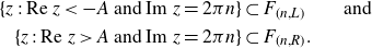
The following theorem is particularly strong when f is of disjoint type, that is, when its Fatou set is an attracting basin and $P(\,f)\subset F(\,f)$
. For each
$P(\,f)\subset F(\,f)$
. For each $R>0$
, we denote
$R>0$
, we denote
 \begin{equation}J_R(\,f)\;:\!=\; \{z\in J(\,f)\colon \vert f^n(z)\vert \geq R \text{ for all } n\geq 1\}.\end{equation}
Theorem 1·3 (Model for cosine dynamics). Let f be a cosine map and let $J(\mathcal{F})$
and
$J(\mathcal{F})$
and $\mathcal{F}$
be as defined as above. Then there exists a constant
$\mathcal{F}$
be as defined as above. Then there exists a constant $R\geq 0$
and a continuous map
$R\geq 0$
and a continuous map $\Phi\colon J(\mathcal{F} )\rightarrow J(\,f)$
such that
$\Phi\colon J(\mathcal{F} )\rightarrow J(\,f)$
such that $\Phi \vert_{\Phi^{-1}(J_R(\,f))}$
is a homeomorphism,
$\Phi \vert_{\Phi^{-1}(J_R(\,f))}$
is a homeomorphism,
 \begin{equation*} \Phi \circ \mathcal{F}=f \circ \Phi \quad \text{ on } \quad \Phi^{-1}(J_R(\,f))\end{equation*}
and $\Phi(I(\,F)) \subset I(\,f)$
. If in addition f is of disjoint type, then
$\Phi(I(\,F)) \subset I(\,f)$
. If in addition f is of disjoint type, then $\Phi\colon J(\mathcal{F})\to J(\,f)$
is a homeomorphism and
$\Phi\colon J(\mathcal{F})\to J(\,f)$
is a homeomorphism and $\Phi(I(\mathcal{F}))=I(\,f).$
Compare to [
Reference Rempe22
, theorems 4·2 and 9·1] for similar results on the exponential family. Note that any escaping point of any cosine map f eventually enters $J_R(\,f)$
for every
$J_R(\,f)$
for every $R>0$
, and so Theorem 1·3 provides a model for its escaping dynamics.
$R>0$
, and so Theorem 1·3 provides a model for its escaping dynamics.
However, we aspire to describe the dynamics of every cosine map in the whole of its Julia set. In particular, in the presence of escaping critical values, any model must reflect the splitting of dynamic rays at (preimages of) critical points, as described for the map $z\mapsto \cosh(z)$
before. Note that our analysis on this map, where each ray tail “splits into two” at critical points, suggests considering two copies of each ray, and mapping each copy to one of the two possible extensions. With that aim, we define the model space for sps maps as
$z\mapsto \cosh(z)$
before. Note that our analysis on this map, where each ray tail “splits into two” at critical points, suggests considering two copies of each ray, and mapping each copy to one of the two possible extensions. With that aim, we define the model space for sps maps as $J(\mathcal{F})_\pm\;:\!=\; J(\mathcal{F})\times \{-,+\}$
with a topology that preserves the circular order of rays at infinity; see Definition 4·6. The model map
$J(\mathcal{F})_\pm\;:\!=\; J(\mathcal{F})\times \{-,+\}$
with a topology that preserves the circular order of rays at infinity; see Definition 4·6. The model map $\widetilde{\mathcal{F}}\colon J(\mathcal{F})_\pm \rightarrow J(\mathcal{F})_\pm$
is defined as
$\widetilde{\mathcal{F}}\colon J(\mathcal{F})_\pm \rightarrow J(\mathcal{F})_\pm$
is defined as $\mathcal{F}$
on the first coordinate and as the identity on the second. Then, our main result is as follows.
$\mathcal{F}$
on the first coordinate and as the identity on the second. Then, our main result is as follows.
Theorem 1·4 (Model for the dynamics of sps cosine maps). Let f be in the cosine family and strongly postcritically separated. Then, there exists a continuous surjective function $\hat{\varphi} \colon J(\mathcal{F})_{\pm} \rightarrow J(\,f)$
so that
$\hat{\varphi} \colon J(\mathcal{F})_{\pm} \rightarrow J(\,f)$
so that $f\circ\hat{\varphi} = \hat{\varphi}\circ \widetilde{\mathcal{F}}$
on
$f\circ\hat{\varphi} = \hat{\varphi}\circ \widetilde{\mathcal{F}}$
on $J(\mathcal{F})_{\pm}$
.
$J(\mathcal{F})_{\pm}$
.
See Theorem 4·7 for a more detailed version of Theorem 1·4. In particular, Theorem 1·2 will follow readily.
Some examples of sps cosine maps that have already appeared in the literature of holomorphic dynamics are $z\mapsto \cosh(z)$
and
$z\mapsto \cosh(z)$
and $z\mapsto \cosh^2(z)$
, see [
Reference Bishop7
,
Reference Martí–Pete and Shishikura12
,
Reference Rippon and Stallard26
]. In Section 5 we improve Theorem 1·4 for these maps by modifying our model as to obtain a conjugacy. In particular, we provide an explicit combinatorial description of the overlap occurring between their dynamic rays and conclude that for both functions, no two of their dynamic rays land together.
$z\mapsto \cosh^2(z)$
, see [
Reference Bishop7
,
Reference Martí–Pete and Shishikura12
,
Reference Rippon and Stallard26
]. In Section 5 we improve Theorem 1·4 for these maps by modifying our model as to obtain a conjugacy. In particular, we provide an explicit combinatorial description of the overlap occurring between their dynamic rays and conclude that for both functions, no two of their dynamic rays land together.
In order to achieve our results on the map $z\mapsto \cosh(z)$
, we introduce the notion of itineraries as sequences that encode the orbits of points on its Julia set with respect to a dynamical partition, an idea already used, for example, in [
Reference Mihaljević–Brandt13
,
Reference Schleicher29
]. In Appendix A, we extend this concept to a larger subclass of functions in
$z\mapsto \cosh(z)$
, we introduce the notion of itineraries as sequences that encode the orbits of points on its Julia set with respect to a dynamical partition, an idea already used, for example, in [
Reference Mihaljević–Brandt13
,
Reference Schleicher29
]. In Appendix A, we extend this concept to a larger subclass of functions in $\mathcal{B}$
with dynamic rays. Namely, to all strongly postcritically separated maps that belong to the class
$\mathcal{B}$
with dynamic rays. Namely, to all strongly postcritically separated maps that belong to the class $\mathcal{CB}$
, the latter including all functions that are a finite composition of class
$\mathcal{CB}$
, the latter including all functions that are a finite composition of class $\mathcal{B}$
functions of finite order. This new tool will allow us to provide in Theorem A12 criteria for their dynamic rays landing together.
$\mathcal{B}$
functions of finite order. This new tool will allow us to provide in Theorem A12 criteria for their dynamic rays landing together.
Structure of the paper. In Section 2 we review some basic properties of cosine dynamics and fix for each cosine map a choice of external addresses, a combinatorial tool used in the study of functions in $\mathcal{B}$
. We define the model
$\mathcal{B}$
. We define the model $(J(\mathcal{F}), \mathcal{F})$
in Section 3, study its properties and prove Theorem 1·3. Section 4 includes our results on sps cosine maps. Namely, we define the model
$(J(\mathcal{F}), \mathcal{F})$
in Section 3, study its properties and prove Theorem 1·3. Section 4 includes our results on sps cosine maps. Namely, we define the model $(J(\mathcal{F})_\pm, \widetilde{\mathcal{F}})$
and prove Theorems 1·4 and 1·2. Next, in Section 5 we sharpen our main result for the maps
$(J(\mathcal{F})_\pm, \widetilde{\mathcal{F}})$
and prove Theorems 1·4 and 1·2. Next, in Section 5 we sharpen our main result for the maps $z \mapsto \cosh(z)$
and
$z \mapsto \cosh(z)$
and $z \mapsto \cosh^2(z)$
and provide a detailed description of their topological dynamics. Finally, we provide combinatorial criteria for dynamic rays of sps functions in
$z \mapsto \cosh^2(z)$
and provide a detailed description of their topological dynamics. Finally, we provide combinatorial criteria for dynamic rays of sps functions in $\mathcal{CB}$
landing together in Appendix A.
$\mathcal{CB}$
landing together in Appendix A.
Basic notation. As used throughout this section, the Fatou, Julia and escaping set of an entire function f are denoted by F(f), J(f) and I(f) respectively. The set of critical values is $\textrm{CV}(\,f)$
, that of asymptotic values is
$\textrm{CV}(\,f)$
, that of asymptotic values is $\textrm{AV}(\,f)$
, and the set of critical points will be
$\textrm{AV}(\,f)$
, and the set of critical points will be $\textrm{Crit}(\,f)$
. The set of singular values of f is S(f), and P(f) denotes the postsingular set. Moreover,
$\textrm{Crit}(\,f)$
. The set of singular values of f is S(f), and P(f) denotes the postsingular set. Moreover, $P_{J}\;:\!=\; P(\,f)\cap J(\,f)$
and
$P_{J}\;:\!=\; P(\,f)\cap J(\,f)$
and $P_{F}\;:\!=\; P(\,f)\cap F(\,f)$
. A disc of radius
$P_{F}\;:\!=\; P(\,f)\cap F(\,f)$
. A disc of radius $\epsilon$
centred at a point p will be
$\epsilon$
centred at a point p will be $\mathbb{D}_\epsilon(p)$
, and
$\mathbb{D}_\epsilon(p)$
, and $\mathbb{C}^\ast \;:\!=\; \mathbb{C}\setminus \{0\}$
. We will indicate the closure of a domain U by
$\mathbb{C}^\ast \;:\!=\; \mathbb{C}\setminus \{0\}$
. We will indicate the closure of a domain U by $\overline{U}$
, that must be understood to be taken in
$\overline{U}$
, that must be understood to be taken in $\mathbb{C}$
. For a holomorphic function f and a set A,
$\mathbb{C}$
. For a holomorphic function f and a set A, $\textrm{Orb}^{-}(A)$
and
$\textrm{Orb}^{-}(A)$
and $\textrm{Orb}^{+}(A)$
are the backward and forward orbit of A under f, respectively. That is,
$\textrm{Orb}^{+}(A)$
are the backward and forward orbit of A under f, respectively. That is, $\textrm{Orb}^{-}(A)\;:\!=\; \bigcup^{\infty}_{n=0} f^{-n}(A)$
and
$\textrm{Orb}^{-}(A)\;:\!=\; \bigcup^{\infty}_{n=0} f^{-n}(A)$
and $\textrm{Orb}^{+}(A)\;:\!=\; \bigcup^{\infty}_{n=0} f^{n}(A).$
2. Cosine dynamics and external addresses
We start by revising basic properties of cosine maps. We refer to [
Reference Rottenfusser, Schleicher, Rippon and Stallard28
,
Reference Schleicher29
] for extensive work on their dynamics. Note also that cosine maps arise as lifts of holomorphic self-maps of $\mathbb{C}^*$
; see [
Reference Fagella and Martí–Pete10
, corollary 1·5]. Recall that for a holomorphic map
$\mathbb{C}^*$
; see [
Reference Fagella and Martí–Pete10
, corollary 1·5]. Recall that for a holomorphic map $f\;:\;\widetilde{S}\rightarrow S$
between Riemann surfaces, the local degree of f at a point
$f\;:\;\widetilde{S}\rightarrow S$
between Riemann surfaces, the local degree of f at a point $z_0\in \widetilde{S}$
, denoted by
$z_0\in \widetilde{S}$
, denoted by $\deg(\,f,z_0)$
, is the unique integer
$\deg(\,f,z_0)$
, is the unique integer $n\geq 1$
such that the local power series development of f is of the form
$n\geq 1$
such that the local power series development of f is of the form
 \begin{equation*}f(z)=f(z_0) + a_n (z-z_0)^n + \text{(higher terms)},\end{equation*}
where $a_n\neq 0$
. Thus,
$a_n\neq 0$
. Thus, $z_0\in \mathbb{C}$
is a critical point of f if and only if
$z_0\in \mathbb{C}$
is a critical point of f if and only if $\deg(\,f,z_0)>1$
. We say that f has bounded criticality on a set A if
$\deg(\,f,z_0)>1$
. We say that f has bounded criticality on a set A if $\textrm{AV}(\,f) \cap A=\emptyset$
and there exists a constant
$\textrm{AV}(\,f) \cap A=\emptyset$
and there exists a constant $M<\infty$
such that
$M<\infty$
such that $\deg(\,f,z)<M \text{ for all } z \in A.$
2·1 (Basic properties of cosine maps). Each cosine map $f(z)\;:\!=\; ae^z+be^{-z}$
with
$f(z)\;:\!=\; ae^z+be^{-z}$
with $a,\,b \in \mathbb{C}^\ast $
is
$a,\,b \in \mathbb{C}^\ast $
is $2\pi i$
-periodic and has exactly two critical values, namely
$2\pi i$
-periodic and has exactly two critical values, namely $\pm 2\sqrt{ab}$
. Furthermore, any preimage of a critical value is a critical point of local degree 2, and hence both critical values are totally ramified. More specifically,
$\pm 2\sqrt{ab}$
. Furthermore, any preimage of a critical value is a critical point of local degree 2, and hence both critical values are totally ramified. More specifically,
 \begin{equation*}\textrm{Crit}(\,f)=\left\{\frac{1}{2}\log\left(\frac{a}{b}\right)+ \pi i n\;:\; n\in \mathbb{Z} \right\},\end{equation*}
where the branch of the logarithm is chosen such that $\vert \textrm{Im} \; ({1}/{2})\log({a}/{b})\vert\leq \pi/2$
. It is easy to check that f has no asymptotic values, and thus,
$\vert \textrm{Im} \; ({1}/{2})\log({a}/{b})\vert\leq \pi/2$
. It is easy to check that f has no asymptotic values, and thus, $S(\,f)\;=\!:\;\{v_1, v_2\}$
, with
$S(\,f)\;=\!:\;\{v_1, v_2\}$
, with $v_i=\pm 2\sqrt{ab}$
and signs chosen so that
$v_i=\pm 2\sqrt{ab}$
and signs chosen so that $v_1$
is the image of
$v_1$
is the image of $({1}/{2})\log({a}/{b})+2\pi i\mathbb{Z}$
, while
$({1}/{2})\log({a}/{b})+2\pi i\mathbb{Z}$
, while $v_2$
is the image of
$v_2$
is the image of $({1}/{2})\log({a}/{b})+\pi i+2\pi i\mathbb{Z}$
. In particular, since S(f) is bounded and f is of order of growth one, the Julia set of any disjoint type cosine map is a Cantor bouquet. Roughly speaking, a Cantor bouquet consists of an uncountable collection of curves to infinity satisfying a certain density condition; see [
Reference Barański, Jarque and Rempe6
, definition 2·1]. Moreover, by the Denjoy–Carleman–Ahlfors theorem, for any choice of bounded domain
$({1}/{2})\log({a}/{b})+\pi i+2\pi i\mathbb{Z}$
. In particular, since S(f) is bounded and f is of order of growth one, the Julia set of any disjoint type cosine map is a Cantor bouquet. Roughly speaking, a Cantor bouquet consists of an uncountable collection of curves to infinity satisfying a certain density condition; see [
Reference Barański, Jarque and Rempe6
, definition 2·1]. Moreover, by the Denjoy–Carleman–Ahlfors theorem, for any choice of bounded domain $D\supset S(\,f)$
, the number of connected components of
$D\supset S(\,f)$
, the number of connected components of $f^{-1}(\mathbb{C} \setminus D)$
, called tracts, is at most two. Note that for any such domain D, f maps points for which the absolute value of their real part is sufficiently large, to
$f^{-1}(\mathbb{C} \setminus D)$
, called tracts, is at most two. Note that for any such domain D, f maps points for which the absolute value of their real part is sufficiently large, to $\mathbb{C} \setminus D$
. Hence, a left and a right half plane are contained in the union of tracts, which implies that f has at least two, and hence exactly two, tracts for any choice of D.
$\mathbb{C} \setminus D$
. Hence, a left and a right half plane are contained in the union of tracts, which implies that f has at least two, and hence exactly two, tracts for any choice of D.
Observation 2·2 (Parameter space of cosine maps). All cosine maps belong to the same parameter space; that is, any two cosine maps are quasiconformally equivalent. To see this, let $f(z)\;:\!=\; ae^z+be^{-z}$
and
$f(z)\;:\!=\; ae^z+be^{-z}$
and $g(z)\;:\!=\; ce^z+de^{-z}$
for
$g(z)\;:\!=\; ce^z+de^{-z}$
for $a,\,b,\,c,\,d \in \mathbb{C}^\ast$
. Consider the linear maps
$a,\,b,\,c,\,d \in \mathbb{C}^\ast$
. Consider the linear maps $\psi(z)\;:\!=\; z+ \log \sqrt{{bc}/{ad}}$
and
$\psi(z)\;:\!=\; z+ \log \sqrt{{bc}/{ad}}$
and $\varphi(z)\;:\!=\; \sqrt{({bc}/{ad})} z$
, which are clearly quasiconformal. Then, for all
$\varphi(z)\;:\!=\; \sqrt{({bc}/{ad})} z$
, which are clearly quasiconformal. Then, for all $z\in \mathbb{C}$
,
$z\in \mathbb{C}$
,
 \begin{equation*} (\,f\circ \psi)(z)=a e^z\sqrt{\frac{bc}{ad}}+be^{-z} \sqrt{\frac{ad}{bc}}=c e^z\sqrt{\frac{ab}{cd}}+de^{-z} \sqrt{\frac{ab}{cd}}=(\varphi\circ g)(z).\end{equation*}
Consequently, in order to prove the second part of Theorem 1·3, by [
Reference Rempe24
, theorem 3·1], it suffices to construct a conjugacy between $\mathcal{F}\colon J(\mathcal{F})\rightarrow J(\mathcal{F})$
and any specific disjoint type cosine map. We could have followed this approach, but for the sake of generality, our proof will relate to any disjoint-type cosine map.
$\mathcal{F}\colon J(\mathcal{F})\rightarrow J(\mathcal{F})$
and any specific disjoint type cosine map. We could have followed this approach, but for the sake of generality, our proof will relate to any disjoint-type cosine map.
Let us fix a cosine function $f(z)\;:\!=\; ae^z+be^{-z}$
with
$f(z)\;:\!=\; ae^z+be^{-z}$
with $a,\,b\in \mathbb{C}^\ast$
. We will make use of some estimates from [
Reference Rottenfusser, Schleicher, Rippon and Stallard28
] that require of constants related to the following:
$a,\,b\in \mathbb{C}^\ast$
. We will make use of some estimates from [
Reference Rottenfusser, Schleicher, Rippon and Stallard28
] that require of constants related to the following:
 \begin{equation*} \mathcal{K}(\,f) \;:\!=\; \!\max \! \left\{\!\left(\sqrt{\left\vert \frac{2b}{a} \right\vert} +\!\sqrt{\left\vert\frac{2a}{b} \right\vert}\right)\!(\vert a \vert + \vert b \vert), 8\vert ab \vert, 1, \frac{1}{2}\ln \left\vert \frac{2b}{a}\right\vert , \frac{1}{2}\ln\left\vert \frac{2a}{b}\right\vert, \ln \frac{16}{\vert a b \vert} \right\}\!. \end{equation*}
More precisely, recall from Section that for any cosine map f and for any choice of Jordan domain $D\supset S(\,f)$
,
$D\supset S(\,f)$
, $f^{-1}(\mathbb{C}\setminus D)$
has two connected components, that is, two tracts. We will choose D large enough as to guarantee Euclidean expansion within tracts, that is, that the modulus of the derivative of any point in the tracts is large enough. Let us choose
$f^{-1}(\mathbb{C}\setminus D)$
has two connected components, that is, two tracts. We will choose D large enough as to guarantee Euclidean expansion within tracts, that is, that the modulus of the derivative of any point in the tracts is large enough. Let us choose $R>\mathcal{K}(\,f)$
big enough such that
$R>\mathcal{K}(\,f)$
big enough such that
 \begin{equation*} \bigcup_{k\in \mathbb{Z}} \{z+2\pi k i \colon z \in \mathbb{D}_R \} \supset \{z \in \mathbb{C} \colon \vert \textrm{Re} \; z \vert\leq \mathcal{K}(\,f)\} \end{equation*}
and $f(\mathbb{D}_R)\supset \mathbb{D}_{\mathcal{K}(\,f)}$
. In particular, the domain
$f(\mathbb{D}_R)\supset \mathbb{D}_{\mathcal{K}(\,f)}$
. In particular, the domain $D\;:\!=\; f(\mathbb{D}_R)$
contains S(f), and so we can define a pair of tracts
$D\;:\!=\; f(\mathbb{D}_R)$
contains S(f), and so we can define a pair of tracts $\mathcal{T}_f$
as the connected components of
$\mathcal{T}_f$
as the connected components of $f^{-1}(\mathbb{C}\setminus D)$
. Then, by definition,
$f^{-1}(\mathbb{C}\setminus D)$
. Then, by definition,
 \begin{equation} \mathcal{T}_f \subseteq \{z\in \mathbb{C} \colon \vert \textrm{Re} \; (z)\vert >\mathcal{K}(\,f) \} \quad \text{ and } \quad S(\,f) \subset \mathbb{D}_{\mathcal{K}(\,f)} \subset \mathbb{C} \setminus f(\mathcal{T}_f).\end{equation}
A simple calculation shows that for any $z\in \mathbb{C}$
such that
$z\in \mathbb{C}$
such that $\vert \textrm{Re} \; z\vert >\mathcal{K}(\,f)$
,
$\vert \textrm{Re} \; z\vert >\mathcal{K}(\,f)$
,
 \begin{equation}\vert f' (z) \vert >2;\end{equation}
see [
Reference Rottenfusser, Schleicher, Rippon and Stallard28
, lemma 3·6]. Hence, we say that $\mathcal{T}_f$
are expansion tracts.
$\mathcal{T}_f$
are expansion tracts.
2·3. (Fundamental domains and inverse branches). Let us fix a cosine map $f(z)\;:\!=\; ae^z+be^{-z}$
for some
$f(z)\;:\!=\; ae^z+be^{-z}$
for some $a,\,b\in \mathbb{C}^\ast$
, and let
$a,\,b\in \mathbb{C}^\ast$
, and let $\mathcal{T}_f$
be a pair of expansion tracts. Let
$\mathcal{T}_f$
be a pair of expansion tracts. Let $S(\,f)\;=\!:\;\{v_1, v_2\}$
, with
$S(\,f)\;=\!:\;\{v_1, v_2\}$
, with $v_1$
and
$v_1$
and $v_2$
labelled according to Section 2·1. In particular, by (2·1),
$v_2$
labelled according to Section 2·1. In particular, by (2·1), $S(\,f)\subset D\;:\!=\; \mathbb{C} \setminus f(\mathcal{T}_f)$
and
$S(\,f)\subset D\;:\!=\; \mathbb{C} \setminus f(\mathcal{T}_f)$
and $\{z\in \mathbb{C} \colon \vert \textrm{Re} \; (z)\vert <\max(\vert \textrm{Re} \; v_1\vert , \vert \textrm{Re} \; v_2 \vert )\}\subset \mathbb{C}\setminus \mathcal{T}_f$
. If
$\{z\in \mathbb{C} \colon \vert \textrm{Re} \; (z)\vert <\max(\vert \textrm{Re} \; v_1\vert , \vert \textrm{Re} \; v_2 \vert )\}\subset \mathbb{C}\setminus \mathcal{T}_f$
. If $\textrm{Im} \; (v_1)> \textrm{Im} \; (v_2)$
, we define
$\textrm{Im} \; (v_1)> \textrm{Im} \; (v_2)$
, we define $\delta$
as the vertical straight line starting at
$\delta$
as the vertical straight line starting at $v_1$
in upwards direction restricted to
$v_1$
in upwards direction restricted to $\mathbb{C}\setminus D$
. If on the contrary
$\mathbb{C}\setminus D$
. If on the contrary $\textrm{Im} \; (v_1)< \textrm{Im} \; (v_2)$
,
$\textrm{Im} \; (v_1)< \textrm{Im} \; (v_2)$
, $\delta$
is the downwards vertical line joining
$\delta$
is the downwards vertical line joining $v_2$
to infinity restricted to
$v_2$
to infinity restricted to $\mathbb{C}\setminus D$
. In any case,
$\mathbb{C}\setminus D$
. In any case, $\delta \subset \mathbb{C}\setminus (\mathcal{T}_f\cup D)$
, and so we can define fundamental domains for f as the connected components of
$\delta \subset \mathbb{C}\setminus (\mathcal{T}_f\cup D)$
, and so we can define fundamental domains for f as the connected components of $\mathcal{T}_f\setminus f^{-1}(\delta)$
; see [
Reference Pardo–Simón18
, section 2] for the definition of fundamental domains in a more general setting. Since f is in the cosine family, by definition, the image of points in
$\mathcal{T}_f\setminus f^{-1}(\delta)$
; see [
Reference Pardo–Simón18
, section 2] for the definition of fundamental domains in a more general setting. Since f is in the cosine family, by definition, the image of points in $\mathbb{R}$
whose modulus is large enough have uniformly large modulus, and so they must be totally contained in a fundamental domain. By
$\mathbb{R}$
whose modulus is large enough have uniformly large modulus, and so they must be totally contained in a fundamental domain. By $2\pi i$
-periodicity of f, the same holds for all their
$2\pi i$
-periodicity of f, the same holds for all their $2\pi i$
-translates. Hence, for each
$2\pi i$
-translates. Hence, for each $n\in \mathbb{Z}$
, we denote by
$n\in \mathbb{Z}$
, we denote by $F_{(n,R)}$
the fundamental domain that contains an unbounded subset of
$F_{(n,R)}$
the fundamental domain that contains an unbounded subset of $2\pi n i + \mathbb{R}^+$
, and by
$2\pi n i + \mathbb{R}^+$
, and by $F_{(n,\,L)}$
the fundamental domain that contains an unbounded subset of
$F_{(n,\,L)}$
the fundamental domain that contains an unbounded subset of $2\pi ni + \mathbb{R}^-$
. Since f maps each fundamental domain to its image
$2\pi ni + \mathbb{R}^-$
. Since f maps each fundamental domain to its image $f(\mathcal{T}_f) \setminus \delta$
as a conformal isomorphism, see [
Reference Pardo Simón17
, proposition 2·19], we can define for each
$f(\mathcal{T}_f) \setminus \delta$
as a conformal isomorphism, see [
Reference Pardo Simón17
, proposition 2·19], we can define for each $(n, \ast) \in \mathbb{Z}\times\{L, R\}$
the inverse branch
$(n, \ast) \in \mathbb{Z}\times\{L, R\}$
the inverse branch
 \begin{equation} f^{-1}_{(n, \ast)}\colon f(\mathcal{T}_f)\setminus \delta \rightarrow F_{(n, \ast)}, \end{equation}
which in particular is a bijection.
Observation 2·4
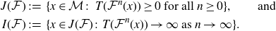
(Horizontal straight lines contained in fundamental domains). Following 2.3, by construction, there is a constant $A>\mathcal{K}(\,f)$
so that for all
$A>\mathcal{K}(\,f)$
so that for all $n\in \mathbb{Z}$
,
$n\in \mathbb{Z}$
,
 \begin{align*} \{z:\; \textrm{Re} \; z<- A \text{ and } \textrm{Im} \; z=2\pi n\} &\subset F_{(n, L)}\qquad\text{and} \\ \{z:\; \textrm{Re} \; z>A \text{ and } \textrm{Im} \; z=2\pi n\} &\subset F_{(n, R)}. \end{align*}
We note that our choice of fundamental domains in Section agrees with the partition defined in [
Reference Rottenfusser, Schleicher, Rippon and Stallard28
, sections 1 and 2], where the maps “ $f^{-1}_{(n, \ast)}$
” are labelled as “
$f^{-1}_{(n, \ast)}$
” are labelled as “ $L_s$
”. Then, the estimates appearing in [
Reference Rottenfusser, Schleicher, Rippon and Stallard28
] regarding this partition and the maps from (2·3) apply to our setting. In particular, we will use the following:
$L_s$
”. Then, the estimates appearing in [
Reference Rottenfusser, Schleicher, Rippon and Stallard28
] regarding this partition and the maps from (2·3) apply to our setting. In particular, we will use the following:
Proposition 2·5 (Properties of the partition [ Reference Rottenfusser, Schleicher, Rippon and Stallard28 , lemmas 2·3 and 3·4]). In the setting described in Section 2·3, the following hold:
-
(i) if
$z,w \in F_{(n,\ast)}$
for some
$(n, \ast) \in \mathbb{Z}\times\{L, R\}$
, then
$\vert \textrm{Im} \; z-\textrm{Im} \; w\vert< 3\pi$
and moreover
$\vert \textrm{Im} \; z-2\pi n\vert< 3\pi$
; -
(ii) if
$w \in f(\mathcal{T}_f) \setminus \delta$
, then for each
$(n, \ast) \in \mathbb{Z}\times\{L, R\}$
there exists
$r^\star\in \mathbb{C}$
with
$\vert r^\star \vert<1$
and such that
\begin{align*} f^{-1}_{(n, \ast)}(w)&\;:\!=\; \left\{\begin{array}{@{}l@{\quad}l@{}} \log(w)-\log a + 2\pi i n + r^\star & \text{ if }\quad \ast=R;\\ -\log(w)+ \log b + 2\pi i n + r^\star & \text{ if }\quad \ast=L. \end{array}\right. \end{align*}


Definition 2·6
(External addresses). Let f be a cosine map. An external address is an infinite sequence ${\underline s}=F_0F_1F_2\ldots$
of the fundamental domains specified in Section 2·3. If
${\underline s}=F_0F_1F_2\ldots$
of the fundamental domains specified in Section 2·3. If ${\underline s}$
is such an external address, we denote
${\underline s}$
is such an external address, we denote
 \begin{equation*} J_{\underline s}= \{z\in J(\,f) \colon f^n(z)\in F_n \text{ for all } n\geq 0\}. \end{equation*}
We let $\textrm{Addr}(\,f)$
be the set of all
$\textrm{Addr}(\,f)$
be the set of all ${\underline s}$
for which
${\underline s}$
for which $J_{\underline s}$
is not empty, that we endow with the usual lexicographic cyclic order topology; see [
Reference Pardo–Simón18
, 2·13] for details.
$J_{\underline s}$
is not empty, that we endow with the usual lexicographic cyclic order topology; see [
Reference Pardo–Simón18
, 2·13] for details.
Observation 2·7. If g is of disjoint type, then $J(g)= \bigcap_{k\geq 0}g^{-k}( \mathcal{T}_g)$
and
$J(g)= \bigcap_{k\geq 0}g^{-k}( \mathcal{T}_g)$
and $g^{-n}(\mathcal{T}_g) \subset \mathcal{T}_g$
for all
$g^{-n}(\mathcal{T}_g) \subset \mathcal{T}_g$
for all $n\geq 0$
; see [
Reference Rempe–Gillen25
, proposition 3·2]. In particular,
$n\geq 0$
; see [
Reference Rempe–Gillen25
, proposition 3·2]. In particular,
 \begin{equation*}J(g)=\bigcup_{{\underline s}\in \textrm{Addr}(g)} J_{\underline s}. \end{equation*}
Notation. For each element $(n, \ast)\in \mathbb{Z}\times\{L, R\}$
, we denote
$(n, \ast)\in \mathbb{Z}\times\{L, R\}$
, we denote $\vert (n, \ast)\vert \;:\!=\; \vert n\vert $
and
$\vert (n, \ast)\vert \;:\!=\; \vert n\vert $
and $\{(n, \ast)\}\;:\!=\; n$
.
$\{(n, \ast)\}\;:\!=\; n$
.
3. A model for cosine dynamics
3.1 (Topological space $(\mathcal{M}, \tau_\mathcal{M})$
). Consider the set
$(\mathcal{M}, \tau_\mathcal{M})$
). Consider the set
 \begin{equation*}\mathcal{M}\;:\!=\; [0,\infty)\times(\mathbb{Z}\times\{L, R\})^\mathbb{N}.\end{equation*}
Let “ $<_{_\mathbb{Z}}$
” be the usual linear order on integers. We define a total order in the set
$<_{_\mathbb{Z}}$
” be the usual linear order on integers. We define a total order in the set $\mathbb{Z}\times\{L, R\}$
as follows:
$\mathbb{Z}\times\{L, R\}$
as follows:
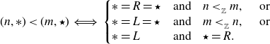 \begin{align} (n,\ast)<(m,\star)& \iff \left\{\begin{array}{@{}l@{\quad}l@{}} \ast=R=\star & \text{and} \quad n<_{_\mathbb{Z}}m, \quad \text{ or }\\ \ast=L=\star & \text{and} \quad m<_{_\mathbb{Z}}n, \quad \text{ or }\\ \ast=L &\text{and} \quad \star=R. \end{array}\right. \end{align}
Then, $<$
induces a lexicographic order “
$<$
induces a lexicographic order “ $<_{\ell}$
” in
$<_{\ell}$
” in $(\mathbb{Z}\times\{L, R\})^\mathbb{N}$
. In turn, we define a cyclic order induced by
$(\mathbb{Z}\times\{L, R\})^\mathbb{N}$
. In turn, we define a cyclic order induced by $<_{\ell}$
in the usual way: for
$<_{\ell}$
in the usual way: for ${\underline s},\underline{\alpha},\underline{\tau} \in (\mathbb{Z}\times\{L, R\})^\mathbb{N}$
,
${\underline s},\underline{\alpha},\underline{\tau} \in (\mathbb{Z}\times\{L, R\})^\mathbb{N}$
,
 \begin{equation*}[{\underline s},\underline{\alpha},\underline{\tau}]_{\ell} \quad \text{if and only if} \quad {\underline s} <_{_\ell}\underline{\alpha}<_{_\ell}\underline{\tau} \quad \text{ or } \quad \underline{\alpha}<_{_\ell} \underline{\tau} <_{_\ell} {\underline s} \quad \text{ or } \quad \underline{\tau} <_{_\ell} {\underline s} <_{_\ell} \underline{\alpha}.\end{equation*}
Moreover, given two different elements ${\underline s},\underline{\tau} \in (\mathbb{Z}\times\{L, R\})^\mathbb{N}$
, we define the open interval from
${\underline s},\underline{\tau} \in (\mathbb{Z}\times\{L, R\})^\mathbb{N}$
, we define the open interval from ${\underline s}$
to
${\underline s}$
to $\underline{\tau}$
, denoted by
$\underline{\tau}$
, denoted by $({\underline s},\underline{\tau})$
, as the set of all points
$({\underline s},\underline{\tau})$
, as the set of all points $x\in (\mathbb{Z}\times\{L, R\})^\mathbb{N}$
such that
$x\in (\mathbb{Z}\times\{L, R\})^\mathbb{N}$
such that $[{\underline s},x,\underline{\tau}]$
. The collection of all such open intervals forms a base for the cyclic order topology. We then provide the space
$[{\underline s},x,\underline{\tau}]$
. The collection of all such open intervals forms a base for the cyclic order topology. We then provide the space $\mathcal{M}$
with the topology
$\mathcal{M}$
with the topology $\tau_\mathcal{M}$
defined as the product topology of
$\tau_\mathcal{M}$
defined as the product topology of $[0, \infty)$
with the usual topology, and
$[0, \infty)$
with the usual topology, and $(\mathbb{Z}\times\{L, R\})^\mathbb{N}$
with the just described cyclic order topology.
$(\mathbb{Z}\times\{L, R\})^\mathbb{N}$
with the just described cyclic order topology.
Notation. If for some $k\geq0$
,
$k\geq0$
, ${\underline s}=s_0s_1s_2\cdots \in (\mathbb{Z}\times\{L, R\})^\mathbb{N}$
is such that
${\underline s}=s_0s_1s_2\cdots \in (\mathbb{Z}\times\{L, R\})^\mathbb{N}$
is such that $s_j=s_k$
for all
$s_j=s_k$
for all $j>k$
, then we write
$j>k$
, then we write ${\underline s}=s_0s_1\cdots \overline{s_k}$
.
${\underline s}=s_0s_1\cdots \overline{s_k}$
.
Observation 3·2 (Correspondence between topological spaces). Let g be any disjoint type cosine map, and let $\textrm{Addr}(g)$
be the set of external addresses, see Definition 2·6. In particular,
$\textrm{Addr}(g)$
be the set of external addresses, see Definition 2·6. In particular, $\textrm{Addr}(g)$
is endowed with a cyclic order topology. We note that there exists a one-to-one correspondence between
$\textrm{Addr}(g)$
is endowed with a cyclic order topology. We note that there exists a one-to-one correspondence between $(\mathbb{Z}\times\{L, R\})^\mathbb{N}$
and
$(\mathbb{Z}\times\{L, R\})^\mathbb{N}$
and $\textrm{Addr}(g)$
that preserves their topologies, namely, the one that converts sequences as follows
$\textrm{Addr}(g)$
that preserves their topologies, namely, the one that converts sequences as follows
 \begin{equation*}(m,\star)(n,\ast)\cdots \leftrightsquigarrow F_{(m,\star)} F_{(n,\ast)}\cdots.\end{equation*}
Since the curve $\delta$
chosen in Section is a vertical straight line, the linear order in fundamental domains chosen to define the cyclic order topology in
$\delta$
chosen in Section is a vertical straight line, the linear order in fundamental domains chosen to define the cyclic order topology in $\textrm{Addr}(g)$
agrees with the linear order (3·1) that determines the topology in
$\textrm{Addr}(g)$
agrees with the linear order (3·1) that determines the topology in $(\mathbb{Z}\times\{L, R\})^\mathbb{N}$
, up to the specified correspondence. Hence, from now on we omit the specification of the correspondence, and
$(\mathbb{Z}\times\{L, R\})^\mathbb{N}$
, up to the specified correspondence. Hence, from now on we omit the specification of the correspondence, and ${\underline s}$
might denote either an element
${\underline s}$
might denote either an element $(m,\star)(n,\ast)\ldots$
of
$(m,\star)(n,\ast)\ldots$
of $(\mathbb{Z}\times\{L, R\})^\mathbb{N}$
, or its corresponding element
$(\mathbb{Z}\times\{L, R\})^\mathbb{N}$
, or its corresponding element $F_{(m,\star)} F_{(n,\ast)}\cdots$
in
$F_{(m,\star)} F_{(n,\ast)}\cdots$
in $\textrm{Addr}(g)$
.
$\textrm{Addr}(g)$
.
Definition 3·3 (A topological model for cosine dynamics). Let $(\mathcal{M}, \tau_\mathcal{M})$
be defined as in Section 3·1. Define
$(\mathcal{M}, \tau_\mathcal{M})$
be defined as in Section 3·1. Define $\mathcal{F} \colon (\mathcal{M},\tau_\mathcal{M}) \to (\mathcal{M},\tau_\mathcal{M})$
as
$\mathcal{F} \colon (\mathcal{M},\tau_\mathcal{M}) \to (\mathcal{M},\tau_\mathcal{M})$
as
 \begin{equation*}\mathcal{F}(t,{\underline s})\;:\!=\;(\,F(t) -2\pi |s_1| , \sigma({\underline s})), \end{equation*}
where $\sigma$
is the shift map on one-sided infinite sequences of
$\sigma$
is the shift map on one-sided infinite sequences of $(\mathbb{Z}\times\{L, R\})^\mathbb{N}$
, and
$(\mathbb{Z}\times\{L, R\})^\mathbb{N}$
, and $F(t)\;:\!=\; e^t-1$
is the standard map that codes exponential growth. Let
$F(t)\;:\!=\; e^t-1$
is the standard map that codes exponential growth. Let $T\colon \mathcal{M} \rightarrow [0, \infty)$
be given by
$T\colon \mathcal{M} \rightarrow [0, \infty)$
be given by $T(t, {\underline s})\;:\!=\; t $
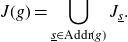
. We set
$T(t, {\underline s})\;:\!=\; t $
. We set
 \begin{align*} J(\mathcal{F}) &\;:\!=\; \{ x\in \mathcal{M} \colon \; T(\mathcal{F}^n(x)) \geq 0 \text{ for all $n\geq 0$}\}, \qquad\text{and} \\ I(\mathcal{F})&\;:\!=\; \{ x \in J(\mathcal{F})\colon T(\mathcal{F}^n(x)) \to \infty \text{ as }n\to\infty \}. \end{align*}
We say that ${\underline s} \in (\mathbb{Z}\times\{L, R\})^{\mathbb{N}}$
is exponentially bounded if
${\underline s} \in (\mathbb{Z}\times\{L, R\})^{\mathbb{N}}$
is exponentially bounded if $(t, {\underline s}) \in J(\mathcal{F})$
for some
$(t, {\underline s}) \in J(\mathcal{F})$
for some $ t>0$
, and denote by
$ t>0$
, and denote by $\mathscr{S}^{\,\mathbb{N}}$
the set of exponentially bounded elements. We moreover let
$\mathscr{S}^{\,\mathbb{N}}$
the set of exponentially bounded elements. We moreover let
 \begin{align*} t_{\underline s}&\;:\!=\; \left\{\begin{array}{@{}l@{\quad}l@{}} \min\{t\geq 0 \;:\; (t, {\underline s}) \in J(\mathcal{F})\} & \text{if } {\underline s} \text{ is exponentially bounded}, \\ \infty & \text{otherwise}. \end{array}\right. \end{align*}
In other words, $J(\mathcal{F})$
is the set of all points that stay in the space
$J(\mathcal{F})$
is the set of all points that stay in the space $\mathcal{M}$
under
$\mathcal{M}$
under $\mathcal{F}^n$
for all
$\mathcal{F}^n$
for all $n\geq 0$
.
$n\geq 0$
.
Remark. Compare to [
Reference Mihaljević–Brandt15
, appendix A], where the construction of a similar model for the map $z \mapsto \pi\sinh(z)$
is sketched.
$z \mapsto \pi\sinh(z)$
is sketched.
Observation 3·4 (Relation between cosine and exponential models). Suppose that the set $\mathbb{Z}^\mathbb{N}$
is endowed with the lexicographical order topology, and define
$\mathbb{Z}^\mathbb{N}$
is endowed with the lexicographical order topology, and define $\mathcal{M}_{\exp}\;:\!=\;[0, \infty) \times \mathbb{Z}^\mathbb{N}$
with the product topology. Moreover, define the map
$\mathcal{M}_{\exp}\;:\!=\;[0, \infty) \times \mathbb{Z}^\mathbb{N}$
with the product topology. Moreover, define the map $\mathcal{F}_{\exp}\colon \mathcal{M}_{\exp}\rightarrow \mathcal{M}_{\exp}$
and the set
$\mathcal{F}_{\exp}\colon \mathcal{M}_{\exp}\rightarrow \mathcal{M}_{\exp}$
and the set $J(\mathcal{F}_{\exp})$
replacing in Definition 3·3 the space
$J(\mathcal{F}_{\exp})$
replacing in Definition 3·3 the space $\mathcal{M}$
by
$\mathcal{M}$
by $\mathcal{M}_{\exp}$
. Then,
$\mathcal{M}_{\exp}$
. Then, $(\mathcal{F}_{\exp}, J(\mathcal{F}_{\exp}))$
is the model for the dynamics of exponential maps described in [
Reference Rempe22
, section 3] and [
Reference Alhabib and Rempe–Gillen2
, definition 3·1]. We note that there does not exist an order preserving bijection between
$(\mathcal{F}_{\exp}, J(\mathcal{F}_{\exp}))$
is the model for the dynamics of exponential maps described in [
Reference Rempe22
, section 3] and [
Reference Alhabib and Rempe–Gillen2
, definition 3·1]. We note that there does not exist an order preserving bijection between $\mathbb{Z}^\mathbb{N}$
with the usual lexicographic order and
$\mathbb{Z}^\mathbb{N}$
with the usual lexicographic order and $((\mathbb{Z}\times\{L, R\})^\mathbb{N}, <_\ell)$
, and hence the models are not the same. This was expected, since exponential maps have a single tract contained on a right half plane, while cosine maps have two tracts, as noted in Section 2·1. However, the spaces
$((\mathbb{Z}\times\{L, R\})^\mathbb{N}, <_\ell)$
, and hence the models are not the same. This was expected, since exponential maps have a single tract contained on a right half plane, while cosine maps have two tracts, as noted in Section 2·1. However, the spaces $\mathcal{M}$
and
$\mathcal{M}$
and $\mathcal{M}_{\exp} \times \{L,R\}^\mathbb{N}$
with the product topology are homeomorphic via the map
$\mathcal{M}_{\exp} \times \{L,R\}^\mathbb{N}$
with the product topology are homeomorphic via the map $h \colon \mathcal{M}_{\exp} \times \{L,R\}^\mathbb{N} \rightarrow \mathcal{M}$
given by
$h \colon \mathcal{M}_{\exp} \times \{L,R\}^\mathbb{N} \rightarrow \mathcal{M}$
given by $h(t,{\underline s},\underline{\omega})\;:\!=\;(t,(s_0,w_0)(s_1,w_1)(s_2,w_2)\ldots)$
, where
$h(t,{\underline s},\underline{\omega})\;:\!=\;(t,(s_0,w_0)(s_1,w_1)(s_2,w_2)\ldots)$
, where ${\underline s}=s_0s_1\cdots \in \mathbb{Z}^N$
and
${\underline s}=s_0s_1\cdots \in \mathbb{Z}^N$
and $\underline{\omega}=w_0w_1w_2\cdots\in \{L,R\}^\mathbb{N}$
. This can be seen by recalling that a base for the product topology of
$\underline{\omega}=w_0w_1w_2\cdots\in \{L,R\}^\mathbb{N}$
. This can be seen by recalling that a base for the product topology of $\mathcal{M}_{\exp} \times \{L,R\}^\mathbb{N}$
is given by cylinders, and the image of each such cylinder under h can be expressed as a union of intervals of
$\mathcal{M}_{\exp} \times \{L,R\}^\mathbb{N}$
is given by cylinders, and the image of each such cylinder under h can be expressed as a union of intervals of $\tau_\mathcal{M}$
, and vice-versa, preimages of intervals are unions of cylinders. In particular,
$\tau_\mathcal{M}$
, and vice-versa, preimages of intervals are unions of cylinders. In particular, $J(\mathcal{F})$
is homeomorphic to
$J(\mathcal{F})$
is homeomorphic to $J(\mathcal{F}_{\exp})\times\{L,R\}^\mathbb{N}$
, where each subspace has the topology respectively induced from
$J(\mathcal{F}_{\exp})\times\{L,R\}^\mathbb{N}$
, where each subspace has the topology respectively induced from $\mathcal{M}$
and
$\mathcal{M}$
and $\mathcal{M}_{\exp} \times \{L,R\}^\mathbb{N}$
.
$\mathcal{M}_{\exp} \times \{L,R\}^\mathbb{N}$
.
We shall use the relation specified above between the exponential and cosine models to prove properties of the latter:
Proposition 3·5 (Properties of the cosine model). The space $J(\mathcal{F})$
with the induced subspace topology admits the 1-point compactification, and the resulting space
$J(\mathcal{F})$
with the induced subspace topology admits the 1-point compactification, and the resulting space $J(\mathcal{F})\cup\{\tilde{\infty}\}$
is a sequential space. Moreover,
$J(\mathcal{F})\cup\{\tilde{\infty}\}$
is a sequential space. Moreover, $\mathcal{F} \vert_{J(\mathcal{F})}$
is continuous.
$\mathcal{F} \vert_{J(\mathcal{F})}$
is continuous.
Proof. By Observation 3·4, $J(\mathcal{F})$
is homeomorphic to
$J(\mathcal{F})$
is homeomorphic to $J(\mathcal{F}_{\exp})\times\{L,R\}^\mathbb{N}$
. In turn,
$J(\mathcal{F}_{\exp})\times\{L,R\}^\mathbb{N}$
. In turn, $J(\mathcal{F}_{\exp})$
is homeomorphic to a straight brush, which is a subset of
$J(\mathcal{F}_{\exp})$
is homeomorphic to a straight brush, which is a subset of $\mathbb{R}^2$
with the usual Euclidean metric, see [
Reference Alhabib and Rempe–Gillen2
, theorem 3·3], and
$\mathbb{R}^2$
with the usual Euclidean metric, see [
Reference Alhabib and Rempe–Gillen2
, theorem 3·3], and $\{L,R\}^\mathbb{N}$
is homeomorphic to the Cantor set. Hence, the product space
$\{L,R\}^\mathbb{N}$
is homeomorphic to the Cantor set. Hence, the product space $J(\mathcal{F}_{\exp})\times\{L,R\}^\mathbb{N}$
is also locally compact and Hausdorff, and so it admits the one-point compactification; see [
Reference Munkres16
, and section 19 and section 29]. Then, as the resulting space is second, and so first, countable, it is a sequential space [
Reference Arkhangel’skiǐ and Fedorchuk5
, definition 9 and proposition 7].
$J(\mathcal{F}_{\exp})\times\{L,R\}^\mathbb{N}$
is also locally compact and Hausdorff, and so it admits the one-point compactification; see [
Reference Munkres16
, and section 19 and section 29]. Then, as the resulting space is second, and so first, countable, it is a sequential space [
Reference Arkhangel’skiǐ and Fedorchuk5
, definition 9 and proposition 7].
In order to prove continuity of $\mathcal{F}\vert_{J(\mathcal{F})}$
, let us fix an arbitrary
$\mathcal{F}\vert_{J(\mathcal{F})}$
, let us fix an arbitrary $(t,{\underline s}) \in J(\mathcal{F})$
and let V be an open neighbourhood of
$(t,{\underline s}) \in J(\mathcal{F})$
and let V be an open neighbourhood of $\mathcal{F}(t, {\underline s})$
. Without loss of generality, we may assume that
$\mathcal{F}(t, {\underline s})$
. Without loss of generality, we may assume that $V=((t_1, t_2)\times \mathcal{I}) \cap J(\mathcal{F})$
for some open interval
$V=((t_1, t_2)\times \mathcal{I}) \cap J(\mathcal{F})$
for some open interval $\mathcal{I} \in (\mathbb{Z}\times \{L, R\})^\mathbb{N}$
and
$\mathcal{I} \in (\mathbb{Z}\times \{L, R\})^\mathbb{N}$
and $t_1, t_2\in \mathbb{R}^+$
so that
$t_1, t_2\in \mathbb{R}^+$
so that $t_1\leq T(\mathcal{F}(t,{\underline s}))< t_2$
. Suppose that
$t_1\leq T(\mathcal{F}(t,{\underline s}))< t_2$
. Suppose that ${\underline s}=s_0s_1\cdots$
and denote
${\underline s}=s_0s_1\cdots$
and denote $\tilde{\mathcal{I}}\;:\!=\; \{s_0\underline{\tau} \;:\; \underline{\tau} \in \mathcal{I}\}$
. In particular,
$\tilde{\mathcal{I}}\;:\!=\; \{s_0\underline{\tau} \;:\; \underline{\tau} \in \mathcal{I}\}$
. In particular, ${\underline s} \in \tilde{\mathcal{I}}$
, and since by definition of
${\underline s} \in \tilde{\mathcal{I}}$
, and since by definition of $\mathcal{F}$
,
$\mathcal{F}$
, $t=\log(T(\mathcal{F}(t, {\underline s}))+1+2\pi\{s_1\})$
and the function
$t=\log(T(\mathcal{F}(t, {\underline s}))+1+2\pi\{s_1\})$
and the function $\log$
is increasing,
$\log$
is increasing,
 \begin{equation*}U\;:\!=\;(\log(t_1+1+2\pi \{s_1\} ), \log(t_2+1+2\pi \{s_1\}))\times \tilde{\mathcal{I}})\cap J(\mathcal{F})\end{equation*}
is an open neighbourhood of $(t,{\underline s})$
such that
$(t,{\underline s})$
such that $\mathcal{F}(U)\subset V.$
In order to prove Theorem 1·3, our main task will be to construct for each disjoint type cosine map g, a continuous map $\Phi\;:\; J(\mathcal{F}) \rightarrow J(g)$
that conjugates the dynamics of
$\Phi\;:\; J(\mathcal{F}) \rightarrow J(g)$
that conjugates the dynamics of $\mathcal{F}$
to those of
$\mathcal{F}$
to those of $g\vert_{ J(g)}$
. Then, the result for any cosine map f will follow using Rempe’s conjugacy between f and g “near infinity”; [
Reference Rempe24
]. In the disjoint type case, the map
$g\vert_{ J(g)}$
. Then, the result for any cosine map f will follow using Rempe’s conjugacy between f and g “near infinity”; [
Reference Rempe24
]. In the disjoint type case, the map $\Phi$
will send each point
$\Phi$
will send each point $(t,\underline{s})\in J(\mathcal{F})$
to a point
$(t,\underline{s})\in J(\mathcal{F})$
to a point $z\in J(g)$
such that
$z\in J(g)$
such that $z\in J_{\underline s}$
and
$z\in J_{\underline s}$
and $ \vert \textrm{Re} \; z\vert \approx\;t$
, see Observation 3·2. We will obtain the map
$ \vert \textrm{Re} \; z\vert \approx\;t$
, see Observation 3·2. We will obtain the map $\Phi$
as the limit of a series of approximations
$\Phi$
as the limit of a series of approximations $\{ \Phi_n\}_{n\in \mathbb{N}}$
; compare [
Reference Mihaljević–Brandt15
,
Reference Pardo–Simón21
,
Reference Rempe22
,
Reference Rempe24
] for similar arguments. The first approximation should be a projection from the space
$\{ \Phi_n\}_{n\in \mathbb{N}}$
; compare [
Reference Mihaljević–Brandt15
,
Reference Pardo–Simón21
,
Reference Rempe22
,
Reference Rempe24
] for similar arguments. The first approximation should be a projection from the space $J(\mathcal{F})$
to the dynamical plane of g.
$J(\mathcal{F})$
to the dynamical plane of g.
Definition 3·6 (Projection function). For each $A\geq 0$
, we define a projection function
$A\geq 0$
, we define a projection function $\mathcal{C}_A\;:\; J(\mathcal{F}) \to \mathbb{C}$
as
$\mathcal{C}_A\;:\; J(\mathcal{F}) \to \mathbb{C}$
as
 \begin{align*} \mathcal{C}_A(t, {\underline s})&\;:\!=\; \left\{\begin{array}{@{}l@{\quad}l@{}} t+A + 2\pi \{s_0\}i & \text{if} \quad s_0=(n,R) \text{ for some }n\in \mathbb{Z}, \\ -t-A+ 2\pi \{s_0\}i & \text{otherwise}, \end{array}\right. \end{align*}
where ${\underline s}=s_0s_1\cdots$
, and if
${\underline s}=s_0s_1\cdots$
, and if $s_0=(n, \ast)$
, then
$s_0=(n, \ast)$
, then $\{s_0\}=\{(n, \ast)\}=n$
.
$\{s_0\}=\{(n, \ast)\}=n$
.
Observation 3·7 (The projection of $J(\mathcal{F})$
lies in fundamental domains). Suppose that g is a disjoint type cosine function for which fundamental domains have been defined following Section 2·3. If A is the constant from Observation 2·4, then
$J(\mathcal{F})$
lies in fundamental domains). Suppose that g is a disjoint type cosine function for which fundamental domains have been defined following Section 2·3. If A is the constant from Observation 2·4, then $\mathcal{C}_A(J(\mathcal{F}))$
is totally contained in the union of fundamental domains. More specifically, for each
$\mathcal{C}_A(J(\mathcal{F}))$
is totally contained in the union of fundamental domains. More specifically, for each $(t, {\underline s})\in J(\mathcal{F})$
, if
$(t, {\underline s})\in J(\mathcal{F})$
, if ${\underline s}=s_0s_1\cdots$
, then
${\underline s}=s_0s_1\cdots$
, then $\mathcal{C}_A(t, {\underline s}) \subset F_{s_0}$
; see also Observation 3·2.
$\mathcal{C}_A(t, {\underline s}) \subset F_{s_0}$
; see also Observation 3·2.
Remark. The reason why instead of projecting under $\mathcal{C}_A$
each point
$\mathcal{C}_A$
each point $(t, {\underline s})\in J(\mathcal{F})$
to a point of real part
$(t, {\underline s})\in J(\mathcal{F})$
to a point of real part $\pm t$
, but rather
$\pm t$
, but rather $\pm t \pm A$
for some constant A, is to ensure that for a fixed function g, the image of each
$\pm t \pm A$
for some constant A, is to ensure that for a fixed function g, the image of each $(t,{\underline s})\in J(\mathcal{F})$
under a projection map lies in a fundamental domain of g, on which, by Proposition 2·5, g expands the Euclidean metric. Note that
$(t,{\underline s})\in J(\mathcal{F})$
under a projection map lies in a fundamental domain of g, on which, by Proposition 2·5, g expands the Euclidean metric. Note that $\mathcal{C}_A(J(\mathcal{F})) \nsubseteq J(g)$
. Nonetheless, since
$\mathcal{C}_A(J(\mathcal{F})) \nsubseteq J(g)$
. Nonetheless, since $\Phi$
will be obtained as the limit of a composition of functions consisting of inverse branches of g whose images lie in
$\Phi$
will be obtained as the limit of a composition of functions consisting of inverse branches of g whose images lie in $\mathcal{T}_g$
, by Observation 2·7, its codomain will be J(g).
$\mathcal{T}_g$
, by Observation 2·7, its codomain will be J(g).
Recall that cosine maps behave like the exponential map for points with modulus large enough and sufficiently far from the imaginary axis. In particular, all such points are contained in fundamental domains. An essential characteristic of our model for cosine dynamics is that, as occurs for the exponential model, for each $(t,{\underline s})\in J(\mathcal{F})$
,
$(t,{\underline s})\in J(\mathcal{F})$
, $\vert \mathcal{C}_A(\mathcal{F}(\underline{s},t))\vert$
is roughly the exponential of its real part. More precisely:
$\vert \mathcal{C}_A(\mathcal{F}(\underline{s},t))\vert$
is roughly the exponential of its real part. More precisely:
Proposition 3·8 (Model acts similar to the exponential). If $(t,{\underline s}) \in J(\mathcal{F})$
and
$(t,{\underline s}) \in J(\mathcal{F})$
and $A>0$
,
$A>0$
,
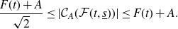 \begin{equation} \frac{F(t)+A}{\sqrt{2}} \leq \vert \mathcal{C}_A(\mathcal{F}(t,{\underline s}))\vert \leq F(t)+A. \end{equation}
Proof. Suppose that ${\underline s}=s_0s_1\cdots $
and let
${\underline s}=s_0s_1\cdots $
and let $b\;:\!=\; 2\pi \{s_1\} $
. Then,
$b\;:\!=\; 2\pi \{s_1\} $
. Then,
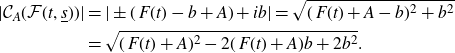 \begin{equation} \begin{split} \vert \mathcal{C}_A(\mathcal{F}(t,{\underline s}))\vert &= \vert \pm(\,F(t)-b+A) + ib \vert=\sqrt{(\,F(t)+A-b)^{2}+ b^2} \\ &=\sqrt{(\,F(t)+A)^{2}-2(\,F(t)+A)b +2b^{2}}. \end{split} \end{equation}
The second inequality in (3·2) follows from the assumption $T(\mathcal{F}(t,{\underline s}))\geq 0$
, that is,
$T(\mathcal{F}(t,{\underline s}))\geq 0$
, that is, $F(t)-b \geq \;0$
, because by (3·3),
$F(t)-b \geq \;0$
, because by (3·3),
 \begin{equation*}\vert \mathcal{C}_A(\mathcal{F}(t,{\underline s}))\vert\leq \sqrt{(\,F(t)+A)^{2}} \iff -2(\,F(t)+A)b +2b^{2}\leq 0 \iff b \leq F(t)+A,\end{equation*}
where we have used that $A,\,b,\,F(t)\geq 0$
. For the first inequality in (3·2), we have
$A,\,b,\,F(t)\geq 0$
. For the first inequality in (3·2), we have
 \begin{equation*} \begin{split} \sqrt{(\,F(t)+A)^{2}} \leq \sqrt{2} \vert \mathcal{C}_A(\mathcal{F}(t,{\underline s}))\vert & \iff (\,F(t)+A)^{2}-4(\,F(t)+A)b +4b^{2} \geq 0 \\ &\iff(\,F(t)+A-2b)^{2}\geq 0. \end{split} \end{equation*}
We describe the underlying idea in the construction of the map $\Phi$
that conjugates
$\Phi$
that conjugates $\mathcal{F}$
to any disjoint type map
$\mathcal{F}$
to any disjoint type map $g\vert_{J(g)}$
. For each
$g\vert_{J(g)}$
. For each $n\geq 0$
, a function
$n\geq 0$
, a function $\Phi_n\colon J(\mathcal{F}) \rightarrow \mathbb{C}$
will be defined the following way: we iterate each point
$\Phi_n\colon J(\mathcal{F}) \rightarrow \mathbb{C}$
will be defined the following way: we iterate each point $x=(t, {\underline s})\in J(\mathcal{F})$
, with
$x=(t, {\underline s})\in J(\mathcal{F})$
, with ${\underline s}=s_0s_1\cdots$
, under the model function
${\underline s}=s_0s_1\cdots$
, under the model function $\mathcal{F}$
a number n of times. In particular,
$\mathcal{F}$
a number n of times. In particular, $\mathcal{F}^n(t, {\underline s})=(t', \sigma^n({\underline s}))$
for some
$\mathcal{F}^n(t, {\underline s})=(t', \sigma^n({\underline s}))$
for some $t'>0$
. Next, we move to the dynamical plane of g using the function
$t'>0$
. Next, we move to the dynamical plane of g using the function $\mathcal{C}_A$
for some constant A big enough such that
$\mathcal{C}_A$
for some constant A big enough such that $(\mathcal{C}_A\circ\mathcal{F}^n)(t, {\underline s})\in F_{s_n}$
. Then, we use the composition of n inverse branches of g specified in (2·3) to obtain a point in
$(\mathcal{C}_A\circ\mathcal{F}^n)(t, {\underline s})\in F_{s_n}$
. Then, we use the composition of n inverse branches of g specified in (2·3) to obtain a point in $F_{s_0}$
, which will define
$F_{s_0}$
, which will define $\Phi_n(x)$
; see Figure 1. Finally, we use (Euclidean) expansion of g on its tracts to show that
$\Phi_n(x)$
; see Figure 1. Finally, we use (Euclidean) expansion of g on its tracts to show that $\{\Phi_n\}_{n\geq 0}$
is a uniformly convergent sequence. We now formalise these ideas:
$\{\Phi_n\}_{n\geq 0}$
is a uniformly convergent sequence. We now formalise these ideas:
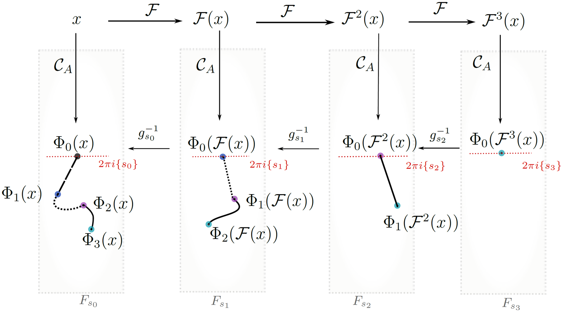
Fig. 1. A schematic of the functions and curves involved in the definition of $\{\Phi_n\}_{n\in \mathbb{N}}$
.
$\{\Phi_n\}_{n\in \mathbb{N}}$
.
Definition 3·9 (Functions $\Phi_n$
). Let g be a disjoint-type cosine map, and let A be a constant provided by Observation 2·4. Then, for each
$\Phi_n$
). Let g be a disjoint-type cosine map, and let A be a constant provided by Observation 2·4. Then, for each $n\geq 0$
we define the function
$n\geq 0$
we define the function $\Phi_{n}\;:\; J(\mathcal{F})\rightarrow \mathbb{C}$
as
$\Phi_{n}\;:\; J(\mathcal{F})\rightarrow \mathbb{C}$
as
 \begin{equation*}\Phi_0(x)\;:\!=\; \mathcal{C}_A(x)\qquad \text{ and }\qquad \Phi_{n+1}(x)\;:\!=\; g^{-1}_{s_0}(\Phi_{n}(\mathcal{F}(x)), \end{equation*}
for $x=(t,{\underline s})$
and
$x=(t,{\underline s})$
and ${\underline s}=s_0s_1\cdots$
.
${\underline s}=s_0s_1\cdots$
.
The function $\Phi_0$
is clearly well-defined. In order to see that for all
$\Phi_0$
is clearly well-defined. In order to see that for all $n\geq 1$
the function
$n\geq 1$
the function $\Phi_n$
is also well-defined, fix
$\Phi_n$
is also well-defined, fix $x=(t, {\underline s})\in J(\mathcal{F})$
and suppose that
$x=(t, {\underline s})\in J(\mathcal{F})$
and suppose that ${\underline s}=s_0s_1\cdots$
. Then, expanding definitions
${\underline s}=s_0s_1\cdots$
. Then, expanding definitions
 \begin{equation}\Phi_{n}(x)= \left(g^{-1}_{s_0}\circ g^{-1}_{s_1} \circ \cdots \circ g^{-1}_{s_{n-1}} \circ \mathcal{C}_A \circ \mathcal{F}^n\right)(x).\end{equation}
By Observations 3·7 and 2·7, the composition of the inverse branches $\{g^{-1}_{s_i}\}_{i< n}$
is well-defined on
$\{g^{-1}_{s_i}\}_{i< n}$
is well-defined on $\mathcal{C}_A(\mathcal{F}^n(x))\in F_{s_n}$
. Moreover, by construction, for all
$\mathcal{C}_A(\mathcal{F}^n(x))\in F_{s_n}$
. Moreover, by construction, for all $n\geq 0$
,
$n\geq 0$
,
 \begin{equation}\Phi_{n}\circ \mathcal{F}= g \circ \Phi_{n+1}.\end{equation}
Proposition 3·10 (Continuity of the functions $\Phi_n$
). For each
$\Phi_n$
). For each $n\geq 0$
,
$n\geq 0$
, $\Phi_n\;\colon\;J(\mathcal{F}) \rightarrow \mathbb{C}$
is continuous.
$\Phi_n\;\colon\;J(\mathcal{F}) \rightarrow \mathbb{C}$
is continuous.
Proof. Let us fix an arbitrary $(t,{\underline s})\in J(\mathcal{F})$
with
$(t,{\underline s})\in J(\mathcal{F})$
with ${\underline s}=s_0s_1\cdots$
, as well as some
${\underline s}=s_0s_1\cdots$
, as well as some $\epsilon>0$
. To see that
$\epsilon>0$
. To see that $\Phi_0\equiv\mathcal{C}_A$
is continuous, let
$\Phi_0\equiv\mathcal{C}_A$
is continuous, let $\mathcal{I} \subset (\mathbb{Z}\times\{L, R\})^\mathbb{N}$
be any open interval containing
$\mathcal{I} \subset (\mathbb{Z}\times\{L, R\})^\mathbb{N}$
be any open interval containing ${\underline s}$
and such that if
${\underline s}$
and such that if $\underline{\tau}=\tau_0\tau_1\cdots \in \mathcal{I}$
, then
$\underline{\tau}=\tau_0\tau_1\cdots \in \mathcal{I}$
, then $s_0=\tau_0$
. Then,
$s_0=\tau_0$
. Then, $U\;:\!=\; \left((t-\epsilon, t+\epsilon) \times \mathcal{I}\right) \cap J(\mathcal{F})$
is an open neighbourhood of
$U\;:\!=\; \left((t-\epsilon, t+\epsilon) \times \mathcal{I}\right) \cap J(\mathcal{F})$
is an open neighbourhood of $(t, {\underline s})$
such that
$(t, {\underline s})$
such that
 \begin{equation*}\mathcal{C}_A(U)\subset (\pm t-\epsilon, \pm t+\epsilon) \pm A + 2\pi i \{s_0\} \subset \mathbb{D}_\epsilon(\pm t\pm A + 2\pi i \{s_0\})= \mathbb{D}_\epsilon(\mathcal{C}_A(t,{\underline s})),\end{equation*}
where $\pm$
equals “
$\pm$
equals “ $+$
” or “ minus;” depending on whether
$+$
” or “ minus;” depending on whether $s_0=(n,R)$
or
$s_0=(n,R)$
or $s_0=(n,\,L)$
for some
$s_0=(n,\,L)$
for some $n\in \mathbb{Z}$
. Hence, we have shown continuity of
$n\in \mathbb{Z}$
. Hence, we have shown continuity of $\Phi_0$
. For each
$\Phi_0$
. For each $n\geq 1$
, let
$n\geq 1$
, let
 \begin{equation*}L_n\;:\!=\; g_{s_0}^{-1} \circ g_{s_1}^{-1} \circ \cdots \circ g^{-1}_{s_{n-1}}\circ \Phi_0 \circ \mathcal{F}^n\end{equation*}
and note that for any subset $U\subset J(\mathcal{F})$
such that
$U\subset J(\mathcal{F})$
such that $\Phi_0(\mathcal{F}^n(U))\subset F_{s_n}$
, by Proposition 3·5 and the definition of the maps
$\Phi_0(\mathcal{F}^n(U))\subset F_{s_n}$
, by Proposition 3·5 and the definition of the maps $\{g^{-1}_{s_i}\}_{i< n}$
,
$\{g^{-1}_{s_i}\}_{i< n}$
, $L_n\vert_{U}$
is a continuous function, as it is a composition of continuous functions. By (3·4),
$L_n\vert_{U}$
is a continuous function, as it is a composition of continuous functions. By (3·4), $L_n(t,{\underline s})=\Phi_n(t,{\underline s})$
. Hence, in order to prove continuity of
$L_n(t,{\underline s})=\Phi_n(t,{\underline s})$
. Hence, in order to prove continuity of $\Phi_n$
at
$\Phi_n$
at $(t,{\underline s})$
, since by Observation 3·7
$(t,{\underline s})$
, since by Observation 3·7 $\Phi_0(\mathcal{F}^n(t,{\underline s}))\subset F_{s_n}$
, it suffices to find a neighbourhood
$\Phi_0(\mathcal{F}^n(t,{\underline s}))\subset F_{s_n}$
, it suffices to find a neighbourhood $V \ni (t,{\underline s})$
such that
$V \ni (t,{\underline s})$
such that $\Phi_{n}\vert_{V} \equiv L_{n}\vert_{V}$
. Let
$\Phi_{n}\vert_{V} \equiv L_{n}\vert_{V}$
. Let $J_n \subset (\mathbb{Z}\times\{L, R\})^\mathbb{N}$
be any open interval containing
$J_n \subset (\mathbb{Z}\times\{L, R\})^\mathbb{N}$
be any open interval containing ${\underline s}$
and such that if
${\underline s}$
and such that if $\underline{\tau}=\tau_0\tau_1\cdots \in J_n$
, then
$\underline{\tau}=\tau_0\tau_1\cdots \in J_n$
, then $s_i=\tau_i$
for all
$s_i=\tau_i$
for all $0\leq i \leq n$
, and choose
$0\leq i \leq n$
, and choose $t_1,t_2\in \mathbb{R}^+$
so that
$t_1,t_2\in \mathbb{R}^+$
so that $t_1\leq t \leq t_2$
. Then,
$t_1\leq t \leq t_2$
. Then, $V\;:\!=\; ((t_1, t_2)\times J_n) \cap J(\mathcal{F})$
satisfies the properties required and continuity of
$V\;:\!=\; ((t_1, t_2)\times J_n) \cap J(\mathcal{F})$
satisfies the properties required and continuity of $\Phi_n$
follows.
$\Phi_n$
follows.
We are now ready to prove Theorem 1·3. We will do so by first showing that for any given disjoint-type cosine map g, the functions $\{\Phi_n\}_{n\in \mathbb{N}}$
converge to a continuous function
$\{\Phi_n\}_{n\in \mathbb{N}}$
converge to a continuous function $\Phi\colon J(\mathcal{F})\to J(g)$
satisfying the properties listed on the second part of the statement. Then, for the first part, given any cosine map f, we will use [
Reference Pardo–Simón19
, theorem 4·6] to relate its dynamics to those of a disjoint-type cosine map, and then apply the second part. We note that [
Reference Pardo–Simón19
, theorem 4·6] relies heavily on Rempe’s analogs of Bottcher’s map for transcendental maps, and more specifically on [
Reference Rempe24
, theorem 3·2].
$\Phi\colon J(\mathcal{F})\to J(g)$
satisfying the properties listed on the second part of the statement. Then, for the first part, given any cosine map f, we will use [
Reference Pardo–Simón19
, theorem 4·6] to relate its dynamics to those of a disjoint-type cosine map, and then apply the second part. We note that [
Reference Pardo–Simón19
, theorem 4·6] relies heavily on Rempe’s analogs of Bottcher’s map for transcendental maps, and more specifically on [
Reference Rempe24
, theorem 3·2].
Proof of Theorem
1·3. We start by showing the second part of the statement. Let g be a disjoint type cosine map and let $\mathcal{T}_g$
be a pair of expansion tracts for g. Let
$\mathcal{T}_g$
be a pair of expansion tracts for g. Let $\{\Phi_{n}\}_{n\geq 0}$
be the sequence of functions from Definition 3·9, and suppose that
$\{\Phi_{n}\}_{n\geq 0}$
be the sequence of functions from Definition 3·9, and suppose that $g(z)=ae^z+ be^{-z}$
for some
$g(z)=ae^z+ be^{-z}$
for some $a,\,b\in \mathbb{C}^\ast$
. If
$a,\,b\in \mathbb{C}^\ast$
. If $M\;:\!=\; \max\{\vert a \vert, \vert b \vert\}$
, then by Propositions 2·5 and 3·8, for each
$M\;:\!=\; \max\{\vert a \vert, \vert b \vert\}$
, then by Propositions 2·5 and 3·8, for each $x=(t, {\underline s}) \in J(\mathcal{F})$
with
$x=(t, {\underline s}) \in J(\mathcal{F})$
with ${\underline s}=s_0s_1s_2\cdots$
,
${\underline s}=s_0s_1s_2\cdots$
,
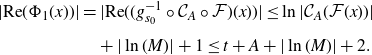 \begin{align*} \vert \textrm{Re} \; ( \Phi_1(x)) \vert & =\vert \textrm{Re} \; ( (g_{s_0}^{-1} \circ \mathcal{C}_A \circ\mathcal{F})(x))\vert \leq \ln\vert \mathcal{C}_A(\mathcal{F}(x)) \vert \\[4pt] & \quad +\vert \ln(M) \vert +1 \leq t+A +\vert\ln(M) \vert+2. \end{align*}
Similarly, $\vert \textrm{Re} \; ( \Phi_1(x)) \vert \geq t-\ln(\sqrt{2})-\vert\ln(M) \vert-2$
. By the definition of
$\vert \textrm{Re} \; ( \Phi_1(x)) \vert \geq t-\ln(\sqrt{2})-\vert\ln(M) \vert-2$
. By the definition of $\Phi_1$
and Observation 2·4, both
$\Phi_1$
and Observation 2·4, both $\Phi_0(x)$
and
$\Phi_0(x)$
and $\Phi_1(x)$
lie in the same fundamental domain
$\Phi_1(x)$
lie in the same fundamental domain $F_{s_0}$
. Thus, either both points have positive real part, of both have negative real part. By this and using that
$F_{s_0}$
. Thus, either both points have positive real part, of both have negative real part. By this and using that $\vert \textrm{Re} \; (\Phi_0(x))\vert = t+A$
, we have
$\vert \textrm{Re} \; (\Phi_0(x))\vert = t+A$
, we have
 \begin{equation} \vert \textrm{Re} \; (\Phi_0(x)) - \textrm{Re} \; (\Phi_1(x))\vert\leq A+\ln(\sqrt{2}) +\vert \ln(M) \vert+2. \end{equation}
Moreover, by (3·6) and Proposition 2·5,
 \begin{equation} \vert \Phi_0(x) -\Phi_1(x)\vert \leq A +\ln(\sqrt{2}) + \vert \ln(M)\vert +2 + 3\pi \;=\!:\;\mu, \end{equation}
where we note that the constant $\mu$
does not depend on the point x. In particular,
$\mu$
does not depend on the point x. In particular, $\Phi_0(x)$
and
$\Phi_0(x)$
and $\Phi_1(x)$
lie in the same tract, and hence the straight segment joining these two points is totally contained in a connected component of
$\Phi_1(x)$
lie in the same tract, and hence the straight segment joining these two points is totally contained in a connected component of $\{z\;:\; \vert \textrm{Re} \; z\vert >\mathcal{K}(g)\}$
, which is a convex set. Moreover, by (3·4), if
$\{z\;:\; \vert \textrm{Re} \; z\vert >\mathcal{K}(g)\}$
, which is a convex set. Moreover, by (3·4), if $\mathsf{g}^{-1}_{{\underline s},n}\;:\!=\; g^{-1}_{s_0}\circ g^{-1}_{s_1} \circ \cdots \circ g^{-1}_{s_{n-1}}$
for some
$\mathsf{g}^{-1}_{{\underline s},n}\;:\!=\; g^{-1}_{s_0}\circ g^{-1}_{s_1} \circ \cdots \circ g^{-1}_{s_{n-1}}$
for some $n\geq 1$
, then
$n\geq 1$
, then
 \begin{equation*}\Phi_n(x)=(\mathsf{g}^{-1}_{{\underline s},n}\circ \Phi_0 \circ \mathcal{F}^n)(x) \quad \text{ and } \quad \Phi_{n+1}(x)=(\mathsf{g}^{-1}_{{\underline s},n}\circ\Phi_1 \circ\mathcal{F}^n)(x).\end{equation*}
Note that if $\gamma$
is the straight segment connecting
$\gamma$
is the straight segment connecting $\Phi_0(\mathcal{F}^n(x))$
and
$\Phi_0(\mathcal{F}^n(x))$
and $\Phi_1(\mathcal{F}^n(x))$
, then since the map
$\Phi_1(\mathcal{F}^n(x))$
, then since the map $\mathsf{g}^{-1}_{{\underline s},n}$
is a bijection to its image as it is a composition of bijections,
$\mathsf{g}^{-1}_{{\underline s},n}$
is a bijection to its image as it is a composition of bijections, $\mathsf{g}^{-1}_{{\underline s},n} (\gamma)$
is a curve with endpoints
$\mathsf{g}^{-1}_{{\underline s},n} (\gamma)$
is a curve with endpoints $\Phi_n(x)$
and
$\Phi_n(x)$
and $\Phi_{n+1}(x)$
. Thus, using (3·7) and (2·2),
$\Phi_{n+1}(x)$
. Thus, using (3·7) and (2·2),
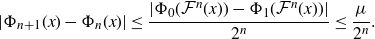 \begin{equation} \vert \Phi_{n+1}(x)-\Phi_n(x)\vert \leq \frac{\vert \Phi_0(\mathcal{F}^n(x)) -\Phi_1(\mathcal{F}^n(x))\vert} {2^n} \leq \frac {\mu} {2^n}. \end{equation}
Hence, $\{\Phi_n\}_{n\geq 0}$
is a uniformly Cauchy sequence of continuous functions, and so they converge uniformly to a continuous limit function
$\{\Phi_n\}_{n\geq 0}$
is a uniformly Cauchy sequence of continuous functions, and so they converge uniformly to a continuous limit function $\Phi\;:\;J(\mathcal{F}) \rightarrow \mathbb{C}$
, that by (3·5) satisfies
$\Phi\;:\;J(\mathcal{F}) \rightarrow \mathbb{C}$
, that by (3·5) satisfies
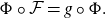 \begin{equation} \Phi\circ \mathcal{F}=g \circ \Phi. \end{equation}
Note that for each $x \in J(\mathcal{F})$
,
$x \in J(\mathcal{F})$
, $\Phi(x)$
is the limit of the backward orbit of a point in
$\Phi(x)$
is the limit of the backward orbit of a point in $\mathcal{T}_g$
, see (3·4). Hence, by Observation 2·7,
$\mathcal{T}_g$
, see (3·4). Hence, by Observation 2·7, $\Phi(x)\in J(g)$
and thus,
$\Phi(x)\in J(g)$
and thus, $\Phi(J(\mathcal{F}))\subset J(g)$
. Moreover, since
$\Phi(J(\mathcal{F}))\subset J(g)$
. Moreover, since $\mathcal{C}_A \equiv \Phi_0$
, for each
$\mathcal{C}_A \equiv \Phi_0$
, for each $x\in J(\mathcal{F})$
,
$x\in J(\mathcal{F})$
,
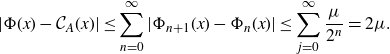 \begin{equation} \vert \Phi(x)-\mathcal{C}_A(x)\vert \leq \sum_{n=0} ^{\infty} \vert\Phi_{n+1}(x)-\Phi_n(x)\vert \leq\sum_{j=0} ^{\infty}\frac{\mu}{2^{n}} =2\mu. \end{equation}
This means for any sequence $\lbrace x_n \rbrace_{n\in \mathbb{N}} \subset J(\mathcal{F})$
that
$\lbrace x_n \rbrace_{n\in \mathbb{N}} \subset J(\mathcal{F})$
that $\Phi(x_n)\rightarrow\infty$
if and only if
$\Phi(x_n)\rightarrow\infty$
if and only if $\mathcal{C}_A(x_n)\rightarrow\infty$
as
$\mathcal{C}_A(x_n)\rightarrow\infty$
as $n\rightarrow \infty$
. By this, the definition of
$n\rightarrow \infty$
. By this, the definition of $I(\mathcal{F})$
and Proposition 3·8,
$I(\mathcal{F})$
and Proposition 3·8,
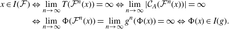 \begin{equation} \begin{split} x \in I(\mathcal{F})& \Leftrightarrow \lim_{n \to \infty} T(\mathcal{F}^n(x))=\infty \Leftrightarrow \lim_{n \to \infty}\vert \mathcal{C}_A(\mathcal{F}^n(x)) \vert =\infty \\ & \Leftrightarrow \lim_{n \to \infty} \Phi(\mathcal{F}^n(x))= \lim_{n \to \infty} g^{n}(\Phi(x))=\infty \Leftrightarrow \Phi(x) \in I(g). \end{split} \end{equation}
Equivalently, $\Phi(I(\mathcal{F})) \subseteq I(g)$
and
$\Phi(I(\mathcal{F})) \subseteq I(g)$
and $\Phi(J(\mathcal{F}) \setminus I(\mathcal{F})) \subseteq J(g)\setminus I(g)$
. Consequently, surjectivity of
$\Phi(J(\mathcal{F}) \setminus I(\mathcal{F})) \subseteq J(g)\setminus I(g)$
. Consequently, surjectivity of $\Phi$
would imply
$\Phi$
would imply $\Phi(I(\mathcal{F})) = I(g).$
Claim. The function $\Phi\;:\; J(\mathcal{F}) \rightarrow J(g)$
is surjective.
$\Phi\;:\; J(\mathcal{F}) \rightarrow J(g)$
is surjective.
Proof of claim. Fix an arbitrary $z\in J(g)$
. Then,
$z\in J(g)$
. Then, $z\in J_{\underline s}$
for some
$z\in J_{\underline s}$
for some ${\underline s}=s_0s_1s_2\cdots \in \textrm{Addr}(g)$
, see Observation 2·7. Note that by definition, the function
${\underline s}=s_0s_1s_2\cdots \in \textrm{Addr}(g)$
, see Observation 2·7. Note that by definition, the function $\mathcal{F}$
is injective on its first coordinate. That is, for each fixed
$\mathcal{F}$
is injective on its first coordinate. That is, for each fixed ${\underline s}\in (\mathbb{Z}\times \{L,R\})^\mathbb{N}$
,
${\underline s}\in (\mathbb{Z}\times \{L,R\})^\mathbb{N}$
, $\mathcal{F}_{{\underline s}}\;:\!=\; \mathcal{F}(\cdot, {\underline s})\colon \mathbb{R}^+\rightarrow \mathbb{C}$
given by
$\mathcal{F}_{{\underline s}}\;:\!=\; \mathcal{F}(\cdot, {\underline s})\colon \mathbb{R}^+\rightarrow \mathbb{C}$
given by $t\mapsto\mathcal{F}(t, {\underline s})$
is injective. Hence, we can consider the sequence of real positive numbers
$t\mapsto\mathcal{F}(t, {\underline s})$
is injective. Hence, we can consider the sequence of real positive numbers $\{t_k\}_{k\geq 0}$
uniquely determined by the equations
$\{t_k\}_{k\geq 0}$
uniquely determined by the equations
 \begin{equation*} \mathcal{F}^{k}(t_k,{\underline s})=(\vert \textrm{Re} \; ( g^{k}(z))\vert, \sigma^{k}({\underline s})). \end{equation*}
In particular, $T(\mathcal{F}^{k}(t_k,{\underline s}))=\vert\textrm{Re} \; (g^{k}(z))\vert>0$
, and hence one can see using a recursive argument that for all
$T(\mathcal{F}^{k}(t_k,{\underline s}))=\vert\textrm{Re} \; (g^{k}(z))\vert>0$
, and hence one can see using a recursive argument that for all $0\leq j\leq k$
,
$0\leq j\leq k$
,
 \begin{equation} T(\mathcal{F}^{j}(t_k,{\underline s}))=\log \left( T(\mathcal{F}^{j+1}(t_k,{\underline s}))+2\pi \{ s_{j+1}\} +1 \right)>0, \end{equation}
and so $\mathcal{F}^j(t_k, {\underline s})$
is indeed well-defined for all
$\mathcal{F}^j(t_k, {\underline s})$
is indeed well-defined for all $j\leq k$
. By definition of the map
$j\leq k$
. By definition of the map $\mathcal{C}_A$
, it holds that
$\mathcal{C}_A$
, it holds that $\textrm{Re} \; ( \mathcal{C}_A(\mathcal{F}^{k}(t_k,{\underline s})))=\pm\textrm{Re} \; (g^{k}(z)) \pm A$
, where “
$\textrm{Re} \; ( \mathcal{C}_A(\mathcal{F}^{k}(t_k,{\underline s})))=\pm\textrm{Re} \; (g^{k}(z)) \pm A$
, where “ $\pm$
” equals “
$\pm$
” equals “ $+$
” or “ minus;” depending on whether
$+$
” or “ minus;” depending on whether $s_k$
belongs to
$s_k$
belongs to $\mathbb{Z}\times \{R\}$
or
$\mathbb{Z}\times \{R\}$
or $\mathbb{Z}\times \{L\}$
. Moreover, by Observation 3·7, both
$\mathbb{Z}\times \{L\}$
. Moreover, by Observation 3·7, both $g^{k}(z),\mathcal{C}_A(\mathcal{F}^{k}(t_k,{\underline s})) \in F_{s_k}$
, and hence by Proposition 2·5,
$g^{k}(z),\mathcal{C}_A(\mathcal{F}^{k}(t_k,{\underline s})) \in F_{s_k}$
, and hence by Proposition 2·5,
 \begin{equation} \vert \mathcal{C}_A(\mathcal{F}^{k}(t_k,{\underline s})) -g^{k}(z) \vert< 3\pi + A. \end{equation}
Note that for all $j\leq k$
, since the second coordinate of
$j\leq k$
, since the second coordinate of $\mathcal{F}^{j}(t_k,{\underline s})$
equals
$\mathcal{F}^{j}(t_k,{\underline s})$
equals $\sigma^j({\underline s})$
, we have that
$\sigma^j({\underline s})$
, we have that $\Phi_{k-j}(\mathcal{F}^{j}(t_k,{\underline s}))=(g^{-1}_{s_{j}}\circ \cdots \circ g^{-1}_{s_{k-1}}\circ \mathcal{C}_A \circ\mathcal{F}^{k})(t_k,{\underline s})$
and
$\Phi_{k-j}(\mathcal{F}^{j}(t_k,{\underline s}))=(g^{-1}_{s_{j}}\circ \cdots \circ g^{-1}_{s_{k-1}}\circ \mathcal{C}_A \circ\mathcal{F}^{k})(t_k,{\underline s})$
and $g^{j}(z)=(g^{-1}_{s_{j}}\circ \cdots \circ g^{-1}_{s_{k-1}}\circ g^k)(z)$
. Hence, using (2·2), (3·10) and (3·13), by the same contraction argument as when showing (3·8), for any
$g^{j}(z)=(g^{-1}_{s_{j}}\circ \cdots \circ g^{-1}_{s_{k-1}}\circ g^k)(z)$
. Hence, using (2·2), (3·10) and (3·13), by the same contraction argument as when showing (3·8), for any $j\leq k$
,
$j\leq k$
,
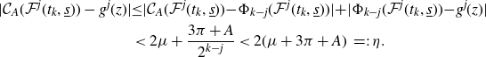 \begin{equation*} \begin{split} \vert \mathcal{C}_A(\mathcal{F}^{j}(t_k,{\underline s})) -g^{j}(z) \vert & \! \leq \! \vert \mathcal{C}_A(\mathcal{F}^{j}(t_k,{\underline s})) \!-\!\Phi_{k-j}(\mathcal{F}^{j}(t_k,{\underline s})) \vert\! + \!\vert \Phi_{k-j}(\mathcal{F}^{j}(t_k,{\underline s}))\!-\!g^j(z)\vert \\ &<2\mu + \frac{3\pi + A}{2^{k-j}}< 2(\mu +3\pi + A)\;=\!:\;\eta. \end{split} \end{equation*}
We note that the constant $\eta$
does not depend on k. In particular, by taking
$\eta$
does not depend on k. In particular, by taking $j=0$
we see that
$j=0$
we see that $t_k$
is uniformly bounded from above by a constant independent of k, and thus
$t_k$
is uniformly bounded from above by a constant independent of k, and thus $t_k\nrightarrow \infty$
as
$t_k\nrightarrow \infty$
as $k \rightarrow \infty$
. This means that there exists at least one finite limit point for the sequence
$k \rightarrow \infty$
. This means that there exists at least one finite limit point for the sequence $\{t_k\}_{k\geq 0}$
, say
$\{t_k\}_{k\geq 0}$
, say $t\geq 0$
, that by (3·12) satisfies
$t\geq 0$
, that by (3·12) satisfies $(t,{\underline s})\in J(\mathcal{F})$
. Since by (3·9), for each
$(t,{\underline s})\in J(\mathcal{F})$
. Since by (3·9), for each $j\geq 0$
, we have
$j\geq 0$
, we have $g^j(\Phi(t,{\underline s}))=\Phi (\mathcal{F}^j(t,{\underline s}))$
,
$g^j(\Phi(t,{\underline s}))=\Phi (\mathcal{F}^j(t,{\underline s}))$
,
 \begin{equation*} \begin{split} \vert g^j(\Phi(t,{\underline s})) -g^{j}(z) \vert \! \leq \!\vert \Phi(\mathcal{F}^j(t,{\underline s}))\!- \!\mathcal{C}_A(\mathcal{F}^{j}(t,{\underline s})) \vert \!+\! \vert \mathcal{C}_A(\mathcal{F}^{j}(t,{\underline s}))-g^j(z)\vert \!< \!2\mu + \eta, \end{split} \end{equation*}
and this upper bound does not depend on j. Since $g^j(\Phi(t,{\underline s}))$
and
$g^j(\Phi(t,{\underline s}))$
and $g^{j}(z)$
belong to the same fundamental domain
$g^{j}(z)$
belong to the same fundamental domain $F_{s_j}$
for each
$F_{s_j}$
for each $j\geq 0$
, we can once more use the same contraction argument to conclude that the points
$j\geq 0$
, we can once more use the same contraction argument to conclude that the points $\Phi(t,{\underline s})$
and z are equal.
$\Phi(t,{\underline s})$
and z are equal.
To prove injectivity of $\Phi$
, note that if
$\Phi$
, note that if $(t,{\underline s}), (t', {\underline s}) \in J(\mathcal{F})$
for some
$(t,{\underline s}), (t', {\underline s}) \in J(\mathcal{F})$
for some $t\neq t'$
, the orbits of
$t\neq t'$
, the orbits of $(t,{\underline s})$
and
$(t,{\underline s})$
and $(t', {\underline s})$
under
$(t', {\underline s})$
under $\mathcal{F}$
will eventually be far apart by definition of
$\mathcal{F}$
will eventually be far apart by definition of $\mathcal{F}$
. Then, by (3·9) and (3·10), so will be the orbits under g of
$\mathcal{F}$
. Then, by (3·9) and (3·10), so will be the orbits under g of $\Phi(t, {\underline s})$
and
$\Phi(t, {\underline s})$
and $\Phi(t', {\underline s})$
, and injectivity follows.
$\Phi(t', {\underline s})$
, and injectivity follows.
Since the compactification $J(\mathcal{F})\cup \{\tilde{\infty}\}$
is by Proposition 3·5 a sequential space, and so is
$J(\mathcal{F})\cup \{\tilde{\infty}\}$
is by Proposition 3·5 a sequential space, and so is $\widehat{\mathbb{C}}\;:\!=\; \mathbb{C} \cup \{\infty\} $
, the notions of continuity and sequential continuity for functions between these spaces are equivalent. Thus, using (3·11), we can extend
$\widehat{\mathbb{C}}\;:\!=\; \mathbb{C} \cup \{\infty\} $
, the notions of continuity and sequential continuity for functions between these spaces are equivalent. Thus, using (3·11), we can extend $\Phi$
to a continuous map
$\Phi$
to a continuous map $\tilde{\Phi}\;:\; J(\mathcal{F}) \cup \lbrace \tilde{\infty} \rbrace \rightarrow J(g) \cup \lbrace \infty \rbrace$
by defining
$\tilde{\Phi}\;:\; J(\mathcal{F}) \cup \lbrace \tilde{\infty} \rbrace \rightarrow J(g) \cup \lbrace \infty \rbrace$
by defining $\tilde{\Phi}(\tilde{\infty})\;:\!=\;\infty$
. Then,
$\tilde{\Phi}(\tilde{\infty})\;:\!=\;\infty$
. Then, $\tilde{\Phi}^{-1}$
is continuous as it is the inverse of a continuous bijective map on a compact space, and consequently, by respectively removing
$\tilde{\Phi}^{-1}$
is continuous as it is the inverse of a continuous bijective map on a compact space, and consequently, by respectively removing $\tilde{\infty}$
and
$\tilde{\infty}$
and $\infty$
from the domain and codomain of
$\infty$
from the domain and codomain of $\tilde{\Phi}^{-1}$
, it follows that
$\tilde{\Phi}^{-1}$
, it follows that $\Phi^{-1}$
is also continuous.
$\Phi^{-1}$
is also continuous.
We have shown that for any cosine map g of disjoint type, $\Phi \colon J(\mathcal{F}) \rightarrow J(g)$
is a homeomorphism and
$\Phi \colon J(\mathcal{F}) \rightarrow J(g)$
is a homeomorphism and $\Phi(I(\,F))=I(g)$
.
$\Phi(I(\,F))=I(g)$
.
Suppose now that f is any cosine map. If follows from [
Reference Pardo–Simón19
, theorem 4·6] that there is a disjoint type cosine map g and a continuous function $\theta\colon J(g)\to J(\,f)$
with the following properties:
$\theta\colon J(g)\to J(\,f)$
with the following properties:
-
(i) the restriction
$\theta\colon \theta^{-1}(J_K(\,f)) \to J_K(\,f)$
is a homeomorphism for some
$K>0$
; -
(ii)
$\theta \circ g=f\circ \theta$
in
$\theta^{-1}(J_K(\,f))$
; -
(iii)
$\theta(I(g))\subset I(\,f)$
.


More specifically, the map g in [
Reference Pardo–Simón19
, theorem 4·6] is of the form $\lambda f$
for some
$\lambda f$
for some $\lambda \in \mathbb{C}\setminus \{0\}$
, and so g is a cosine map. Then, [
Reference Pardo–Simón19
, theorem 4·6] states that J(g) contains a so-called strongly absorbing Cantor bouquet X, [
Reference Pardo–Simón19
, definition 1·5], such that
$\lambda \in \mathbb{C}\setminus \{0\}$
, and so g is a cosine map. Then, [
Reference Pardo–Simón19
, theorem 4·6] states that J(g) contains a so-called strongly absorbing Cantor bouquet X, [
Reference Pardo–Simón19
, definition 1·5], such that $\theta\vert_X$
is a homeomorphism to its image, [
Reference Pardo–Simón19
, theorem 4·6(d)], and so that
$\theta\vert_X$
is a homeomorphism to its image, [
Reference Pardo–Simón19
, theorem 4·6(d)], and so that $\theta(X)\supset J_K(\,f)$
for some
$\theta(X)\supset J_K(\,f)$
for some $K>0$
, [
Reference Pardo–Simón19
, line 18 in the proof of theorem 4·6]. Thus, (1) follows. Item (2) is a consequence of this together with [
Reference Pardo–Simón19
, theorem 4·6(b)], and (3) is part of [
Reference Pardo–Simón19
, theorem 4·6(g)]. Then, if
$K>0$
, [
Reference Pardo–Simón19
, line 18 in the proof of theorem 4·6]. Thus, (1) follows. Item (2) is a consequence of this together with [
Reference Pardo–Simón19
, theorem 4·6(b)], and (3) is part of [
Reference Pardo–Simón19
, theorem 4·6(g)]. Then, if $\tilde{\Phi}\colon J(\mathcal{F}) \rightarrow J(g)$
is the homeomorphism provided by the second part of the statement, the composition
$\tilde{\Phi}\colon J(\mathcal{F}) \rightarrow J(g)$
is the homeomorphism provided by the second part of the statement, the composition $\Phi \;:\!=\; \theta\circ \tilde{\Phi} \colon J(\mathcal{F})\to J(\,f)$
satisfies the desired properties.
$\Phi \;:\!=\; \theta\circ \tilde{\Phi} \colon J(\mathcal{F})\to J(\,f)$
satisfies the desired properties.
Observation 3·11. Recall from Observation 2·7 that if g is of disjoint type, then $J(g)=\bigcup_{{\underline s}\in \textrm{Addr}(g)} J_{\underline s}$
. It follows from the proof of Theorem 1·3 that in this case, for each
$J(g)=\bigcup_{{\underline s}\in \textrm{Addr}(g)} J_{\underline s}$
. It follows from the proof of Theorem 1·3 that in this case, for each ${\underline s}\in \textrm{Addr}(g)$
,
${\underline s}\in \textrm{Addr}(g)$
, $\Phi\colon \{(t, {\underline s}) \colon t \geq t_{\underline s}\} \to J_{\underline s}$
is a bijection, see also Observation 3·2. This implies that
$\Phi\colon \{(t, {\underline s}) \colon t \geq t_{\underline s}\} \to J_{\underline s}$
is a bijection, see also Observation 3·2. This implies that $\Phi$
acts as an order-preserving map from
$\Phi$
acts as an order-preserving map from $\mathscr{S}^{\,\mathbb{N}}$
to
$\mathscr{S}^{\,\mathbb{N}}$
to $\textrm{Addr}(g)$
. Note also that
$\textrm{Addr}(g)$
. Note also that $J(\mathcal{F})$
is a straight brush, see the proof of Proposition 3·5, and in particular a collection of disjoint unbounded curves. Hence, our result provides another proof of the fact that J(g) is a Cantor bouquet.
$J(\mathcal{F})$
is a straight brush, see the proof of Proposition 3·5, and in particular a collection of disjoint unbounded curves. Hence, our result provides another proof of the fact that J(g) is a Cantor bouquet.
4. A model for strongly postcritically separated cosine maps
We defined in the introduction what it means for a cosine map to be strongly postcritically separated. This notion, introduced in [
Reference Pardo–Simón20
], generalizes to some functions in class $\mathcal{B}$
:
$\mathcal{B}$
:
Definition 4·1
(Strongly postcritically separated functions). A function $f\in \mathcal{B}$
is strongly postcritically separated (sps) if there are constants
$f\in \mathcal{B}$
is strongly postcritically separated (sps) if there are constants $c,\epsilon >0$
such that:
$c,\epsilon >0$
such that:
-
(i)
$P_{F}\;:\!=\; P(\,f)\cap F(\,f)$
is compact; -
(ii) f has bounded criticality on J(f);
-
(iii) for each
$z\in J(\,f)$
,
$\#(\textrm{Orb}^+(z)\cap \textrm{Crit}(\,f)) \leq c$
; -
(iv) for all distinct
$z,w\in P_J\;:\!=\; P(\,f)\cap J(\,f)$
,
$\vert z-w\vert\geq \epsilon \max\{\vert z \vert, \vert w \vert\}$
.


For cosine maps, some conditions in the definition of strongly postcritically separated maps are trivially satisfied, and thus they can be characterised the following way:
Proposition 4·2 (Cosine maps that are strongly postcritically separated). Let f be in the cosine family. Then the following are equivalent:
-
(i) f is strongly postcritically separated;
-
(ii)
$P_F$
is compact and there exists
$\epsilon>0$
such that for all distinct
$z,w\in P_J$
, (4·1)
\begin{equation} \vert z-w\vert\geq \epsilon \max\{\vert z \vert, \vert w \vert\}. \end{equation}
-
(iii) each critical value of f converges to an attracting cycle or a repelling periodic cycle, or its orbit tends to infinity in such a way that (4·1) holds.


Proof. By definition, (i) $\Rightarrow$
(ii). For any cosine map f,
$\Rightarrow$
(ii). For any cosine map f, $\textrm{AV}(\,f)=\emptyset$
and any critical point has local degree equal to 2, see Section 2·1. In particular, f has bounded criticality on its Julia set. Moreover, since each cosine map has two critical values, for all
$\textrm{AV}(\,f)=\emptyset$
and any critical point has local degree equal to 2, see Section 2·1. In particular, f has bounded criticality on its Julia set. Moreover, since each cosine map has two critical values, for all $z\in J(\,f)$
,
$z\in J(\,f)$
, $\#(\textrm{Orb}^+(z)\cap \textrm{Crit}(\,f)) \leq 2$
. Hence, if f is in the cosine family and (ii) holds for f, then all conditions in the definition of strongly postcritically separated maps (Definition 4·1) are satisfied, and so (ii)
$\#(\textrm{Orb}^+(z)\cap \textrm{Crit}(\,f)) \leq 2$
. Hence, if f is in the cosine family and (ii) holds for f, then all conditions in the definition of strongly postcritically separated maps (Definition 4·1) are satisfied, and so (ii) $\Rightarrow$
(i). If (4·1) holds for f, then
$\Rightarrow$
(i). If (4·1) holds for f, then $P(\,f)\cap J(\,f)$
is discrete. In addition, since
$P(\,f)\cap J(\,f)$
is discrete. In addition, since $f\in \mathcal{B}$
, when
$f\in \mathcal{B}$
, when $P_J$
is discrete,
$P_J$
is discrete, $P_F$
being compact is equivalent to all periodic cycles in J(f) being repelling and F(f) being a collection of attracting basins (see the proof of [
Reference Pardo–Simón20
, lemma 2·6]), and thus, (ii)
$P_F$
being compact is equivalent to all periodic cycles in J(f) being repelling and F(f) being a collection of attracting basins (see the proof of [
Reference Pardo–Simón20
, lemma 2·6]), and thus, (ii) $\Leftrightarrow$
(iii).
$\Leftrightarrow$
(iii).
Remark. The definition that we gave in the introduction of sps cosine maps (Definition 1·1) agrees with Proposition 4·2(ii).
In this section we prove our main results on sps cosine maps; namely, Theorems 1·2 and Section 1·4. We start by providing a formal definition of dynamic rays:
Definition 4·3 (Dynamic rays for transcendental maps [
Reference Rottenfusser, Rückert, Rempe and Schleicher27
, definition 2·2]). Let f be a transcendental entire function. A ray tail of f is an injective curve $\gamma\;:\;[t_0,\infty)\rightarrow I(\,f)$
, with
$\gamma\;:\;[t_0,\infty)\rightarrow I(\,f)$
, with $t_0>0$
, such that:
$t_0>0$
, such that:
-
(i) for each
$n\geq 1$
,
$t \mapsto f^{n}(\gamma(t))$
is injective with
$\lim_{t \rightarrow \infty} f^{n}(\gamma(t))=\infty$
; -
(ii)
$f^{n}(\gamma(t))\rightarrow \infty$
uniformly in t as
$n\rightarrow \infty$
.


A dynamic ray of f is a maximal injective curve $\gamma\;:\;(0,\infty)\rightarrow I(\,f)$
such that the restriction
$\gamma\;:\;(0,\infty)\rightarrow I(\,f)$
such that the restriction $\gamma_{|[t,\infty)}$
is a ray tail for all
$\gamma_{|[t,\infty)}$
is a ray tail for all $t > 0$
. We say that
$t > 0$
. We say that $\gamma$
lands at z if
$\gamma$
lands at z if $\lim_{t \rightarrow 0^+} \gamma(t)=z$
, and we call z the endpoint of
$\lim_{t \rightarrow 0^+} \gamma(t)=z$
, and we call z the endpoint of $\gamma$
. We denote the set of endpoints of dynamic rays of f by E(f).
$\gamma$
. We denote the set of endpoints of dynamic rays of f by E(f).
Recall from the introduction that whenever a ray tail contains a critical value, its preimages can be interpreted as several ray tails that split or break at critical points, and that may be extended to overlap pairwise. In [
Reference Pardo–Simón18
], combinatorics for maps exhibiting this phenomenon are developed, where the extensions of ray tails at critical points, as described for the map $z \mapsto \cosh(z)$
, are formalised.
$z \mapsto \cosh(z)$
, are formalised.
More precisely, let f be a cosine map, let $\textrm{Addr}(\,f)$
be the set of external addresses as specified in Definition 2·6 and denote
$\textrm{Addr}(\,f)$
be the set of external addresses as specified in Definition 2·6 and denote
 \begin{equation}\textrm{Addr}(\,f)_\pm\;:\!=\; \textrm{Addr}(\,f)\times \{-,+\}.\end{equation}
We call each of its elements $({\underline s}, \ast) \in \textrm{Addr}(\,f)_\pm$
a signed (external) address.
$({\underline s}, \ast) \in \textrm{Addr}(\,f)_\pm$
a signed (external) address.
It is shown in [
Reference Pardo–Simón18
, section 3] that $\textrm{Addr}(\,f)_\pm$
can be endowed with a topology such that each
$\textrm{Addr}(\,f)_\pm$
can be endowed with a topology such that each $z\in I(\,f)$
has at least two signed addresses that depend continuously on z. This leads to a folliation of I(f) as a collection of rays, that we call canonical, indexed by signed external addresses. More precisely, we shall use the following results from [
Reference Pardo–Simón18
].
$z\in I(\,f)$
has at least two signed addresses that depend continuously on z. This leads to a folliation of I(f) as a collection of rays, that we call canonical, indexed by signed external addresses. More precisely, we shall use the following results from [
Reference Pardo–Simón18
].
Definition and Theorem 4.4 (Canonical rays). Let f be a sps cosine map. Then, for each $({\underline s}, \ast) \in \textrm{Addr}(\,f)_\pm$
there is a curve
$({\underline s}, \ast) \in \textrm{Addr}(\,f)_\pm$
there is a curve $\Gamma({\underline s}, \ast)$
, that is either a ray tail or a dynamic ray possibly with its endpoint, such that
$\Gamma({\underline s}, \ast)$
, that is either a ray tail or a dynamic ray possibly with its endpoint, such that
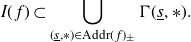 \begin{equation}I(\,f)\subset \bigcup_{({\underline s},\ast)\in \textrm{Addr}(\,f)_\pm} \Gamma({\underline s}, \ast). \end{equation}
We say that $\Gamma({\underline s}, \ast)$
is a canonical ray, and we call any ray tail contained in a canonical ray a canonical tail. Landing of all canonical rays implies landing of all dynamic rays in J(f). Each
$\Gamma({\underline s}, \ast)$
is a canonical ray, and we call any ray tail contained in a canonical ray a canonical tail. Landing of all canonical rays implies landing of all dynamic rays in J(f). Each $z\in I(\,f)$
belongs to exactly
$z\in I(\,f)$
belongs to exactly
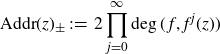 \begin{equation}\textrm{Addr}(z)_\pm \;:\!=\; 2\prod^{\infty}_{j=0}\deg(\,f,f^{j}(z))\end{equation}
different canonical rays, for $\textrm{Addr}(z)_\pm \in \{2,4,8\}.$
Proof. The definition and existence of canonical rays, as well as (4·3), are a consequence of [
Reference Pardo–Simón18
, definition 3·5 and theorem 3·8], while landing of canonical rays implying landing of all dynamic rays is [
Reference Pardo–Simón18
, observation 3·13]. Equation (4·4) follows from [
Reference Pardo–Simón18
, definition 3·10 and observation 3·11], and $\textrm{Addr}(z)_\pm \in \{2,4,8\}$
is a consequence of cosine maps having only 2 critical values, with all critical points being of local degree 2.
$\textrm{Addr}(z)_\pm \in \{2,4,8\}$
is a consequence of cosine maps having only 2 critical values, with all critical points being of local degree 2.
Remark. It follows from the previous result that in order to study dynamic rays for the functions we consider, it suffices to study canonical rays.
Next, we define our model for sps cosine maps. We start by setting the topology we shall use in the ambient space $\mathcal{M}\times \{-,+\}$
that contains
$\mathcal{M}\times \{-,+\}$
that contains $J(\mathcal{F})\times \{-,+\}$
:
$J(\mathcal{F})\times \{-,+\}$
:
4·5 (Definition of topologies). Consider the set
 \begin{equation} \mathcal{M}_\pm \;:\!=\; \mathcal{M}\times \{-,+\}= [0,\infty)\times(\mathbb{Z}\times\{L, R\})^\mathbb{N} \times \{-,+\}, \end{equation}
and let $<_{\ell}$
denote the lexicographic order in
$<_{\ell}$
denote the lexicographic order in $(\mathbb{Z}\times\{L, R\})^\mathbb{N}$
defined in 3.1. Let us give the set
$(\mathbb{Z}\times\{L, R\})^\mathbb{N}$
defined in 3.1. Let us give the set $\lbrace -,+\rbrace$
the order
$\lbrace -,+\rbrace$
the order $\lbrace -\rbrace \prec\lbrace +\rbrace$
, and define the linear order in
$\lbrace -\rbrace \prec\lbrace +\rbrace$
, and define the linear order in $(\mathbb{Z}\times\{L, R\})^\mathbb{N} \times \{-,+\}$
 \begin{equation} (\underline{s}, \ast )<_{_A} (\underline{\tau}, \star) \qquad \text{ if and only if } \qquad \underline{s} <_{_\ell} \underline{\tau} \quad \text{ or } \quad \underline{s} =_{_\ell} \underline{\tau}\: \text{ and } \: \ast \prec \star,\end{equation}
where the symbols “ $\ast, \star$
” denote generic elements of
$\ast, \star$
” denote generic elements of $\lbrace-, +\rbrace.$
This linear order gives rise to a cyclic order: for
$\lbrace-, +\rbrace.$
This linear order gives rise to a cyclic order: for $a,\,x,\,b \in (\mathbb{Z}\times\{L, R\})^\mathbb{N} \times \{-,+\}$
,
$a,\,x,\,b \in (\mathbb{Z}\times\{L, R\})^\mathbb{N} \times \{-,+\}$
,
 \begin{equation*} [a,\,x,\,b]_{_A} \quad \text{if and only if} \quad a<_{_A} x<_{_A} b \quad \text{ or } \quad x <_{_A}b <_{_A} a \quad \text{ or }\quad b <_{_A} a <_{_A} x.\end{equation*}
This cyclic order allows us to provide the set $(\mathbb{Z}\times\{L, R\})^\mathbb{N} \times \{-,+\}$
with the corresponding cyclic order topology
$(\mathbb{Z}\times\{L, R\})^\mathbb{N} \times \{-,+\}$
with the corresponding cyclic order topology $\tau_I$
.
$\tau_I$
.
We define the topological space $(\mathcal{M}_\pm, \tau_{\mathcal{M}_\pm})$
, with
$(\mathcal{M}_\pm, \tau_{\mathcal{M}_\pm})$
, with $\tau_{\mathcal{M}_\pm}$
being the product topology of
$\tau_{\mathcal{M}_\pm}$
being the product topology of $[0,\infty)$
with the usual topology, and
$[0,\infty)$
with the usual topology, and $(\mathbb{Z}\times\{L, R\})^\mathbb{N} \times \{-,+\}$
with the topology
$(\mathbb{Z}\times\{L, R\})^\mathbb{N} \times \{-,+\}$
with the topology $\tau_I$
.
$\tau_I$
.
Definition 4·6 (Model for sps cosine functions). Let $J(\mathcal{F})_\pm\;:\!=\; J(\mathcal{F})\times \{-,+\}$
be the subspace of
$J(\mathcal{F})_\pm\;:\!=\; J(\mathcal{F})\times \{-,+\}$
be the subspace of $\mathcal{M}_\pm$
with the induced topology
$\mathcal{M}_\pm$
with the induced topology $\tau_{\pm}$
from
$\tau_{\pm}$
from $\tau_{\mathcal{M}_\pm}$
. We call
$\tau_{\mathcal{M}_\pm}$
. We call $(J(\mathcal{F})_\pm, \tau_{\pm})$
the model space for strongly postcritically separated cosine maps. Define
$(J(\mathcal{F})_\pm, \tau_{\pm})$
the model space for strongly postcritically separated cosine maps. Define $I(\mathcal{F})_{\pm}\;:\!=\; I(\mathcal{F})\times \lbrace -,+\rbrace \subset J(\mathcal{F})_{\pm}$
as a subspace equipped with the induced topology. We define the model function as
$I(\mathcal{F})_{\pm}\;:\!=\; I(\mathcal{F})\times \lbrace -,+\rbrace \subset J(\mathcal{F})_{\pm}$
as a subspace equipped with the induced topology. We define the model function as $\widetilde{\mathcal{F}}\;:\;J(\mathcal{F})_\pm \to J(\mathcal{F})_\pm$
, given by
$\widetilde{\mathcal{F}}\;:\;J(\mathcal{F})_\pm \to J(\mathcal{F})_\pm$
, given by $\widetilde{\mathcal{F}}(t,{\underline s}, \ast) \;:\!=\;(\mathcal{F}(t,{\underline s}), \ast)$
.
$\widetilde{\mathcal{F}}(t,{\underline s}, \ast) \;:\!=\;(\mathcal{F}(t,{\underline s}), \ast)$
.
We are now ready to prove the main result of this paper, which is a more detailed version of Theorem 1·4. Using the general framework developed in [
Reference Pardo–Simón21
], its proof will be concise. We remark that, alternatively, we could had provided a more direct but significantly more lengthy and technical proof. More precisely, one could avoid using the results from [
Reference Pardo–Simón21
] and construct directly the semiconjugacy from $\mathcal{F}$
to
$\mathcal{F}$
to $f\vert _{J(\,f)}$
in a similar manner to the proof of [
Reference Rottenfusser, Rückert, Rempe and Schleicher27
, theorem 6·5], using that sps maps expand an orbifold metric in a neighbourhood of their Julia sets; [
Reference Pardo–Simón20
, theorem 1·1]. We have opted for the first approach for clarity of exposition and to show an application of the framework that [
Reference Pardo–Simón21
] provides.
$f\vert _{J(\,f)}$
in a similar manner to the proof of [
Reference Rottenfusser, Rückert, Rempe and Schleicher27
, theorem 6·5], using that sps maps expand an orbifold metric in a neighbourhood of their Julia sets; [
Reference Pardo–Simón20
, theorem 1·1]. We have opted for the first approach for clarity of exposition and to show an application of the framework that [
Reference Pardo–Simón21
] provides.
Recall from Definition 3·3 that $\mathscr{S}^{\,\mathbb{N}}$
denotes the set of exponentially bounded elements associated to
$\mathscr{S}^{\,\mathbb{N}}$
denotes the set of exponentially bounded elements associated to $J(\mathcal{F})$
. We define
$J(\mathcal{F})$
. We define $\mathscr{S}^{\,\mathbb{N}}_\pm \;:\!=\;\mathscr{S}^{\,\mathbb{N}}\times \{-,+\}$
.
$\mathscr{S}^{\,\mathbb{N}}_\pm \;:\!=\;\mathscr{S}^{\,\mathbb{N}}\times \{-,+\}$
.
Theorem 4·7. Let f be a strongly postcritically separated cosine map and let $J(\mathcal{F})_\pm$
and
$J(\mathcal{F})_\pm$
and $\widetilde{\mathcal{F}}$
be the model space and function from Definition 4·6. Then,
$\widetilde{\mathcal{F}}$
be the model space and function from Definition 4·6. Then, $\widetilde{\mathcal{F}}$
is continuous, and there exists a continuous surjective function
$\widetilde{\mathcal{F}}$
is continuous, and there exists a continuous surjective function
 \begin{equation*} \hat{\varphi} \colon J(\mathcal{F})_{\pm} \longrightarrow J(\,f) \qquad \text{ so that } \qquad f\circ\hat{\varphi} = \hat{\varphi}\circ \widetilde{\mathcal{F}},\end{equation*} $\hat{\varphi}(I(\mathcal{F})_{\pm})=I(\,f)$
and such that for every
$\hat{\varphi}(I(\mathcal{F})_{\pm})=I(\,f)$
and such that for every $z\in I(\,f)$
,
$z\in I(\,f)$
, $\# \hat{\varphi}^{-1}(z)\in \{2,4,8\}$
. Moreover, for each
$\# \hat{\varphi}^{-1}(z)\in \{2,4,8\}$
. Moreover, for each $({\underline s}, \ast) \in \mathscr{S}^{\,\mathbb{N}}_\pm$
the restriction map
$({\underline s}, \ast) \in \mathscr{S}^{\,\mathbb{N}}_\pm$
the restriction map $\hat{\varphi} \colon \{(t, {\underline s}, \ast) \colon t \geq t_{\underline s}\} \rightarrow \overline{\Gamma({\underline s}, \ast)}$
is a bijection, and so
$\hat{\varphi} \colon \{(t, {\underline s}, \ast) \colon t \geq t_{\underline s}\} \rightarrow \overline{\Gamma({\underline s}, \ast)}$
is a bijection, and so $\overline{\Gamma({\underline s}, \ast)}$
is a canonical ray together with its endpoint.
$\overline{\Gamma({\underline s}, \ast)}$
is a canonical ray together with its endpoint.
Remark. We have implicitly stated in Theorem 4·7 that the map $\hat{\varphi}$
establishes a one-to-one correspondence between
$\hat{\varphi}$
establishes a one-to-one correspondence between $\mathscr{S}^{\,\mathbb{N}}_\pm$
and
$\mathscr{S}^{\,\mathbb{N}}_\pm$
and $\textrm{Addr}(\,f)_\pm$
, since, with some abuse of notation, we have stated that for each
$\textrm{Addr}(\,f)_\pm$
, since, with some abuse of notation, we have stated that for each $({\underline s}, \ast) \in \mathscr{S}^{\,\mathbb{N}}_\pm$
,
$({\underline s}, \ast) \in \mathscr{S}^{\,\mathbb{N}}_\pm$
, $\{(t, {\underline s}, \ast) \colon t \geq t_{\underline s}\}$
is mapped bijectively to
$\{(t, {\underline s}, \ast) \colon t \geq t_{\underline s}\}$
is mapped bijectively to $\overline{\Gamma({\underline s}, \ast)} \subset J(\,f)$
for
$\overline{\Gamma({\underline s}, \ast)} \subset J(\,f)$
for $({\underline s}, \ast) \in \textrm{Addr}(\,f)_\pm$
. In particular, we are claiming that
$({\underline s}, \ast) \in \textrm{Addr}(\,f)_\pm$
. In particular, we are claiming that $\hat{\varphi}$
is an order-preserving continuous map.
$\hat{\varphi}$
is an order-preserving continuous map.
Proof of Theorem
4·7. Let $g\;:\!=\; \lambda f$
be of disjoint type for some
$g\;:\!=\; \lambda f$
be of disjoint type for some $\lambda\in \mathbb{C}^\ast$
and let
$\lambda\in \mathbb{C}^\ast$
and let $\Phi\colon J(\mathcal{F})\to J(g)$
be the homeomorphism from Theorem 1·3. Define
$\Phi\colon J(\mathcal{F})\to J(g)$
be the homeomorphism from Theorem 1·3. Define $J(g)_\pm\;:\!=\; J(g)\times \{-,+\}.$
In [
Reference Pardo–Simón21
, 5·4, p. 23],
$J(g)_\pm\;:\!=\; J(g)\times \{-,+\}.$
In [
Reference Pardo–Simón21
, 5·4, p. 23], $J(g)_\pm$
is induced with a topology
$J(g)_\pm$
is induced with a topology $\tau_J$
in an analogous manner as we did in 4.5 for
$\tau_J$
in an analogous manner as we did in 4.5 for $J(\mathcal{F})_\pm$
, with
$J(\mathcal{F})_\pm$
, with $(\mathbb{Z}\times\{L, R\})^\mathbb{N}$
replaced by
$(\mathbb{Z}\times\{L, R\})^\mathbb{N}$
replaced by $\mathbb{R}\setminus \mathbb{Q}$
in [
Reference Pardo–Simón21
, equation (5·1)]. In particular,
$\mathbb{R}\setminus \mathbb{Q}$
in [
Reference Pardo–Simón21
, equation (5·1)]. In particular,
 \begin{equation} \hat{\Phi}\colon J(\mathcal{F})_\pm\rightarrow J(g)_\pm; \quad \quad (t,{\underline s},\ast)\mapsto (\Phi(t, {\underline s}), \ast) \end{equation}
is a homeomorphism. We let $I(g)_\pm\;:\!=\; I(g)\times \{-,+\}$
and for each
$I(g)_\pm\;:\!=\; I(g)\times \{-,+\}$
and for each ${\underline s}\in \textrm{Addr}(g)$
, denote
${\underline s}\in \textrm{Addr}(g)$
, denote $J_{({\underline s}, \ast)}\;:\!=\; J_{\underline s}\times \{\ast\}$
. Let
$J_{({\underline s}, \ast)}\;:\!=\; J_{\underline s}\times \{\ast\}$
. Let $\tilde{g}\colon J(g)_\pm\rightarrow J(g)_\pm$
be given by
$\tilde{g}\colon J(g)_\pm\rightarrow J(g)_\pm$
be given by $\tilde{g}(z, \ast)\;:\!=\;(g(z), \ast).$
Note that by definition of the functions involved and Theorem 1·3, we have that
$\tilde{g}(z, \ast)\;:\!=\;(g(z), \ast).$
Note that by definition of the functions involved and Theorem 1·3, we have that
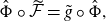 \begin{equation}\hat{\Phi}\circ \widetilde{\mathcal{F}}=\tilde{g} \circ \hat{\Phi},\end{equation}
and, in particular, $\mathcal{F}$
is continuous as it can be expressed as a composition of continuous functions.
$\mathcal{F}$
is continuous as it can be expressed as a composition of continuous functions.
Then, by [
Reference Pardo–Simón21
, theorem 6·5], there exists a continuous, surjective map $\varphi\;:\; J(g)_\pm \to J(\,f)$
such that
$\varphi\;:\; J(g)_\pm \to J(\,f)$
such that
 \begin{equation} f\circ\varphi = \varphi\circ \tilde{g}, \quad \quad \varphi(I(g)_{ \pm})=I(\,f)\end{equation}
and for each $({\underline s}, \ast)\in \textrm{Addr}(g)_\pm$
,
$({\underline s}, \ast)\in \textrm{Addr}(g)_\pm$
,
 \begin{equation}\varphi \colon J_{({\underline s}, \ast)} \rightarrow \overline{\Gamma({\underline s}, \ast)} \quad \text{is a bijection},\end{equation}
where $\Gamma({\underline s}, \ast)$
is the canonical ray at signed address
$\Gamma({\underline s}, \ast)$
is the canonical ray at signed address $({\underline s}, \ast)\in \textrm{Addr}(\,f)_\pm$
. It then follows from Definition and Theorem 4.4 that for each
$({\underline s}, \ast)\in \textrm{Addr}(\,f)_\pm$
. It then follows from Definition and Theorem 4.4 that for each $z\in I(\,f)$
,
$z\in I(\,f)$
,
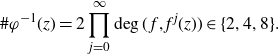 \begin{equation} \#\varphi^{-1}(z)=2\prod^{\infty}_{j=0}\deg(\,f,f^{j}(z))\in \{2,4,8\}.\end{equation}
Let $\hat{\varphi}\;:\!=\;\varphi\circ \hat{\Phi}\;:\; J(\mathcal{F})_\pm \rightarrow J(\,f)$
, which is continuous as it is a composition of continuous functions. Then, by (4·9) and (4·8),
$\hat{\varphi}\;:\!=\;\varphi\circ \hat{\Phi}\;:\; J(\mathcal{F})_\pm \rightarrow J(\,f)$
, which is continuous as it is a composition of continuous functions. Then, by (4·9) and (4·8),
 \begin{equation*}f \circ \hat{\varphi}=f \circ \varphi \circ \hat{\Phi} =\varphi\circ \tilde{g} \circ \hat{\Phi}= \varphi\circ \hat{\Phi}\circ \widetilde{\mathcal{F}}= \hat{\varphi} \circ \widetilde{\mathcal{F}},\end{equation*}
as shown in the diagram:
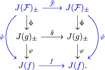
Moreover, since, by Theorem 1·3, $\Phi(I(\mathcal{F}))=I(g)$
, we have that
$\Phi(I(\mathcal{F}))=I(g)$
, we have that $\hat{\Phi}(I(\mathcal{F})_\pm)=I(g)_\pm$
, and consequently
$\hat{\Phi}(I(\mathcal{F})_\pm)=I(g)_\pm$
, and consequently $\hat{\varphi}(I(\mathcal{F})_\pm)=I(\,f)$
.
$\hat{\varphi}(I(\mathcal{F})_\pm)=I(\,f)$
.
Since $\hat{\Phi}$
is a homeomorphism, using (4·11) we have that
$\hat{\Phi}$
is a homeomorphism, using (4·11) we have that $\#\hat{\varphi}^{-1}(z)=\#\varphi^{-1}(z)\in \{2,4,8\}$
. By Observation 3·11,
$\#\hat{\varphi}^{-1}(z)=\#\varphi^{-1}(z)\in \{2,4,8\}$
. By Observation 3·11, $\Phi\colon \{(t, {\underline s}) \colon t \geq t_{\underline s}\} \to J_{\underline s}$
is a bijection for each
$\Phi\colon \{(t, {\underline s}) \colon t \geq t_{\underline s}\} \to J_{\underline s}$
is a bijection for each ${\underline s}\in \mathscr{S}^{\,\mathbb{N}}$
, with
${\underline s}\in \mathscr{S}^{\,\mathbb{N}}$
, with $J_{\underline s}$
being a landing dynamic ray. Hence, by (4·7) and (4·10),
$J_{\underline s}$
being a landing dynamic ray. Hence, by (4·7) and (4·10), $\hat{\varphi} \colon \{(t, {\underline s}, \ast) \colon t \geq t_{\underline s}\} \rightarrow \overline{\Gamma({\underline s}, \ast)}$
is also bijection and
$\hat{\varphi} \colon \{(t, {\underline s}, \ast) \colon t \geq t_{\underline s}\} \rightarrow \overline{\Gamma({\underline s}, \ast)}$
is also bijection and $\overline{\Gamma({\underline s}, \ast)}$
is a canonical ray together with its endpoint.
$\overline{\Gamma({\underline s}, \ast)}$
is a canonical ray together with its endpoint.
Proof of Theorem
1·2. Let f be a sps cosine map. Then, by Definition and Theorem 4.4, proving that all canonical rays of f land suffices to conclude that all its dynamic rays land. Since, by Theorem 4·7, for each $({\underline s}, \ast) \in \textrm{Addr}(\,f)_\pm$
,
$({\underline s}, \ast) \in \textrm{Addr}(\,f)_\pm$
, $\overline{\Gamma({\underline s}, \ast)}$
is a canonical ray together with its landing point, the result follows. Moreover, by Theorem 4·7,
$\overline{\Gamma({\underline s}, \ast)}$
is a canonical ray together with its landing point, the result follows. Moreover, by Theorem 4·7,
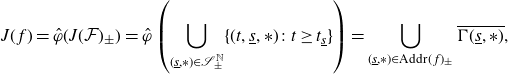 \begin{equation*}J(\,f)=\hat{\varphi}(J(\mathcal{F})_\pm)= \hat{\varphi}\left(\bigcup_{({\underline s}, \ast) \in \mathscr{S}^{\,\mathbb{N}}_\pm}\{(t, {\underline s}, \ast) \colon t \geq t_{\underline s}\}\right)= \bigcup_{({\underline s}, \ast) \in \textrm{Addr}(\,f)_\pm} \overline{\Gamma({\underline s},\ast)},\end{equation*}
and so every point in J(f) is either on a dynamic ray or it is the landing point of at least one such ray.
5. Combinatorics and landing of rays for
$f(z)=\cosh(z)$

In the previous section we provided a semiconjugacy between the restriction of any strongly postcritically separated cosine map f to its Julia set, and a simple dynamical system formed by a map $\widetilde{\mathcal{F}}$
and a model space
$\widetilde{\mathcal{F}}$
and a model space $J(\mathcal{F})_\pm$
, that reflects the splitting of dynamic rays at critical points. In particular, Theorem 4·7 implies that J(f) can be described as a collection of canonical rays that land, and overlap pairwise.
$J(\mathcal{F})_\pm$
, that reflects the splitting of dynamic rays at critical points. In particular, Theorem 4·7 implies that J(f) can be described as a collection of canonical rays that land, and overlap pairwise.
Given the explicit nature of cosine maps, we claim that it is possible to improve this result by providing a conjugacy rather than a semiconjugacy between a model dynamical system and our maps. Note that if a cosine map f is sps, we let $\hat{\varphi} \colon J(\mathcal{F})_{\pm} \rightarrow J(\,f)$
be the map from Theorem 4·7, and we define the equivalence relation in
$\hat{\varphi} \colon J(\mathcal{F})_{\pm} \rightarrow J(\,f)$
be the map from Theorem 4·7, and we define the equivalence relation in $J(\mathcal{F})_\pm$
 \begin{equation}a \sim b \iff \hat{\varphi}(a)=\hat{\varphi}(b),\end{equation}
then, since $\hat{\varphi}$
is continuous, by the Universal Property of Quotient Maps (see for example [
Reference Munkres16
, theorem 2·22]), there exists a unique continuous function
$\hat{\varphi}$
is continuous, by the Universal Property of Quotient Maps (see for example [
Reference Munkres16
, theorem 2·22]), there exists a unique continuous function $\tilde{\varphi}\colon J(\mathcal{F})_\pm /{\sim} \rightarrow J(\,f)$
such that the diagram
$\tilde{\varphi}\colon J(\mathcal{F})_\pm /{\sim} \rightarrow J(\,f)$
such that the diagram
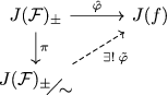
commutes, where $\pi$
is the projection function that takes each element to its equivalence class. In particular, since both
$\pi$
is the projection function that takes each element to its equivalence class. In particular, since both $\hat{\varphi}$
and
$\hat{\varphi}$
and $\pi$
are surjective,
$\pi$
are surjective, $\tilde{\varphi}$
is by definition bijective. By the commutative relation
$\tilde{\varphi}$
is by definition bijective. By the commutative relation $f\circ \hat{\varphi}= \hat{\varphi} \circ \widetilde{\mathcal{F}}$
from Theorem 4·7, for any
$f\circ \hat{\varphi}= \hat{\varphi} \circ \widetilde{\mathcal{F}}$
from Theorem 4·7, for any $a,\,b\in J(\mathcal{F})_\pm$
,
$a,\,b\in J(\mathcal{F})_\pm$
,
 \begin{equation*}\pi(a)=\pi(b) \Rightarrow \hat{\varphi}(\widetilde{\mathcal{F}}(a)) =f(\hat{\varphi}(a))=f(\hat{\varphi}(b))=\hat{\varphi}(\widetilde{\mathcal{F}}(b))\Rightarrow \pi(\widetilde{\mathcal{F}}(a))=\pi(\widetilde{\mathcal{F}}(b)),\end{equation*}
and so, the map $h\colon J(\mathcal{F})_\pm /{\sim} \rightarrow J(\mathcal{F})_\pm /{\sim}$
given by
$h\colon J(\mathcal{F})_\pm /{\sim} \rightarrow J(\mathcal{F})_\pm /{\sim}$
given by $h(\pi(x))\;:\!=\; \pi(\widetilde{\mathcal{F}}(x))$
is a well-defined homeomorphism. In particular,
$h(\pi(x))\;:\!=\; \pi(\widetilde{\mathcal{F}}(x))$
is a well-defined homeomorphism. In particular, $\tilde{\varphi}$
conjugates h and f as shown in the following diagram:
$\tilde{\varphi}$
conjugates h and f as shown in the following diagram:
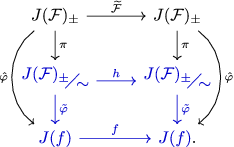
In this section, we describe “ $\sim$
” explicitly for the maps
$\sim$
” explicitly for the maps $z\mapsto \cosh(z)$
and
$z\mapsto \cosh(z)$
and $z\mapsto \cosh^2(z).$
The following observation is important to us.
$z\mapsto \cosh^2(z).$
The following observation is important to us.
Observation 5·1. Recall from Theorem 4·7 that $\hat{\varphi} (\{(t, {\underline s}, \ast) \colon t \geq t_{\underline s}\})= \overline{\Gamma({\underline s}, \ast)}$
for each
$\hat{\varphi} (\{(t, {\underline s}, \ast) \colon t \geq t_{\underline s}\})= \overline{\Gamma({\underline s}, \ast)}$
for each $({\underline s}, \ast)\in \textrm{Addr}(\,f)_\pm$
. Hence, in order to describe
$({\underline s}, \ast)\in \textrm{Addr}(\,f)_\pm$
. Hence, in order to describe $J(\mathcal{F})_\pm /{\sim}$
, we can equivalently determine the overlap occuring between the canonical rays
$J(\mathcal{F})_\pm /{\sim}$
, we can equivalently determine the overlap occuring between the canonical rays $\{\overline{\Gamma({\underline s}, \ast)}\}_{({\underline s}, \ast)\in \textrm{Addr}(\,f)_\pm}$
with their endpoints.
$\{\overline{\Gamma({\underline s}, \ast)}\}_{({\underline s}, \ast)\in \textrm{Addr}(\,f)_\pm}$
with their endpoints.
We will divide our task into two: on one hand, we shall study whether canonical rays share their endpoints, that is, whether some of them land together. On the other hand, one should provide information on the overlaps occuring between canonical rays. For the second, we will use the following result, which is [
Reference Pardo–Simón18
, proposition 3·9]. We recall that $\sigma \colon \textrm{Addr}(\,f)\rightarrow \textrm{Addr}(\,f) $
denotes the one-sided shift map on addresses.
$\sigma \colon \textrm{Addr}(\,f)\rightarrow \textrm{Addr}(\,f) $
denotes the one-sided shift map on addresses.
Proposition 5·2 (Overlapping of canonical rays). For each $({\underline s}, \ast) \in {Addr}(\,f)_\pm$
, either
$({\underline s}, \ast) \in {Addr}(\,f)_\pm$
, either $\Gamma({\underline s}, -)=\Gamma({\underline s}, +)$
when
$\Gamma({\underline s}, -)=\Gamma({\underline s}, +)$
when ${Orb}^{-}({Crit}(\,f)) \cap \Gamma({\underline s}, \ast) =\emptyset$
, or
${Orb}^{-}({Crit}(\,f)) \cap \Gamma({\underline s}, \ast) =\emptyset$
, or $\Gamma({\underline s}, \ast)$
can be expressed as a concatenation
$\Gamma({\underline s}, \ast)$
can be expressed as a concatenation
 \begin{equation} \Gamma({\underline s}, \ast)=\cdots {\cdot} \{c_{i+1}\}{\cdot} \gamma^{i+1}_{i} {\cdot} \{c_i\} {\cdot} \cdots {\cdot}\gamma^{1}_{0} {\cdot} \{c_0\} {\cdot} \gamma^{\infty}_{c_0}, \end{equation}
where $\{c_i\}_{i\in I}={Orb}^{-}({Crit}(\,f)) \cap \Gamma({\underline s}, \ast)$
, for each
$\{c_i\}_{i\in I}={Orb}^{-}({Crit}(\,f)) \cap \Gamma({\underline s}, \ast)$
, for each $i\geq 1$
, if it exists, the curve
$i\geq 1$
, if it exists, the curve $\gamma^{i+1}_{i}$
is a (bounded) piece of dynamic ray, and
$\gamma^{i+1}_{i}$
is a (bounded) piece of dynamic ray, and $\gamma^{\infty}_{c_0}$
is a piece of dynamic ray joining
$\gamma^{\infty}_{c_0}$
is a piece of dynamic ray joining $c_0$
to infinity. In particular, in the latter case, the following properties hold for
$c_0$
to infinity. In particular, in the latter case, the following properties hold for $\Gamma({\underline s}, \ast)$
:
$\Gamma({\underline s}, \ast)$
:
-
(i)
$\gamma^{\infty}_{c_0} \cup \{c_0\}= \Gamma({\underline s},- ) \cap \Gamma({\underline s}, +)$
and
$\gamma^{\infty}_{c_0}$
does not belong to any other canonical ray; -
(ii) for each
$i\geq 0$
, the point
$c_i$
belongs to exactly
$2 \prod^{\infty}_{j=0}\deg(\,f,f^{j}(c_i))$
canonical rays; -
(iii) for each
$i\geq 0$
,
$\gamma^{i+1}_i= \Gamma({\underline s}, \ast)\cap \Gamma(\underline{\tau}, \star)$
, where
$\star\neq \ast$
and
$\sigma^j(\underline{\tau})=\sigma^j({\underline s})$
for some
$j\geq 1$
. Moreover,
$\gamma^{i+1}_i$
does not belong to any other canonical ray.


We start our analysis on the map $f(z)=\cosh(z)$
. Following Observation 5·1, we shall provide a combinatorial description of the equivalence classes of
$f(z)=\cosh(z)$
. Following Observation 5·1, we shall provide a combinatorial description of the equivalence classes of $J(\mathcal{F})_\pm /{\sim}$
in terms of the signed addresses of their images under
$J(\mathcal{F})_\pm /{\sim}$
in terms of the signed addresses of their images under $\tilde{\varphi}$
.
$\tilde{\varphi}$
.
For a function $f\in \mathcal{B}$
, the partition of a neighbourhood of infinity into fundamental domains is commonly regarded as a static partition in the sense that the curve
$f\in \mathcal{B}$
, the partition of a neighbourhood of infinity into fundamental domains is commonly regarded as a static partition in the sense that the curve $\delta$
and domain
$\delta$
and domain $D\supset S(\,f)$
in its definition do not have dynamical meaning for f. In particular, dynamic rays of f might cross the boundaries of fundamental domains infinitely often. Instead, for our specific example, we can define a dynamical partition, so that the boundaries of the components are ray tails:
$D\supset S(\,f)$
in its definition do not have dynamical meaning for f. In particular, dynamic rays of f might cross the boundaries of fundamental domains infinitely often. Instead, for our specific example, we can define a dynamical partition, so that the boundaries of the components are ray tails:
5·3 (Dynamical partition for $f(z)=\cosh(z)$
). For the function
$f(z)=\cosh(z)$
). For the function $f(z)\;:\!=\; \cosh(z)$
,
$f(z)\;:\!=\; \cosh(z)$
, $J(\,f)=\mathbb{C}$
and
$J(\,f)=\mathbb{C}$
and $S(\,f)=\textrm{CV}(\,f)=\{-1, 1\}$
. Moreover, the curves
$S(\,f)=\textrm{CV}(\,f)=\{-1, 1\}$
. Moreover, the curves $\gamma_1\;:\!=\; \mathbb{R} \setminus (-\infty, 1)$
and
$\gamma_1\;:\!=\; \mathbb{R} \setminus (-\infty, 1)$
and $\gamma_{-1}\;:\!=\; \mathbb{R} \setminus (\!-\!1, \infty)$
are ray tails joining 1 and
$\gamma_{-1}\;:\!=\; \mathbb{R} \setminus (\!-\!1, \infty)$
are ray tails joining 1 and $-1$
to
$-1$
to $\infty$
whose forward orbits lie in
$\infty$
whose forward orbits lie in $\mathbb{R}^+$
. Let
$\mathbb{R}^+$
. Let
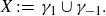 \begin{equation}X\;:\!=\;\gamma_1\cup \gamma_{-1}.\end{equation}
Since $\mathbb{C} \setminus X$
is simply-connected and
$\mathbb{C} \setminus X$
is simply-connected and $S(\,f)\subset X$
, by the Monodromy Theorem, each connected component of
$S(\,f)\subset X$
, by the Monodromy Theorem, each connected component of $f^{-1}(\mathbb{C} \setminus X)$
is a simply-connected domain, and the restriction of f to it is a conformal isomorphism to its image. More specifically, noting that all preimages of the critical values of f are critical points of local degree 2, each connected component of
$f^{-1}(\mathbb{C} \setminus X)$
is a simply-connected domain, and the restriction of f to it is a conformal isomorphism to its image. More specifically, noting that all preimages of the critical values of f are critical points of local degree 2, each connected component of $f^{-1}(\mathbb{C} \setminus X)$
is a horizontal strip of the form
$f^{-1}(\mathbb{C} \setminus X)$
is a horizontal strip of the form
 \begin{equation*} U_K\;:\!=\; \{ z\in \mathbb{C} \text{ such that } K\pi < \textrm{Im} \; z <(K+1)\pi) \} \end{equation*}
for some $K\in\mathbb{Z}$
. We denote
$K\in\mathbb{Z}$
. We denote $\mathcal{U}\;:\!=\; \{U_K\}_{K\in \mathbb{Z}}$
; see Figure 3.
$\mathcal{U}\;:\!=\; \{U_K\}_{K\in \mathbb{Z}}$
; see Figure 3.
5·4 (Fixing signed addresses for $f(z)=\cosh(z)$
). Let us fix any bounded domain
$f(z)=\cosh(z)$
). Let us fix any bounded domain $D\supset [-1,1] \supset S(\,f)$
. Then,
$D\supset [-1,1] \supset S(\,f)$
. Then, $f^{-1}(\mathbb{C}\setminus D)$
consists of two unbounded domains that do not contain the imaginary axis, since
$f^{-1}(\mathbb{C}\setminus D)$
consists of two unbounded domains that do not contain the imaginary axis, since $f(i\mathbb{R})=[-1,1]$
. Thus, we can choose
$f(i\mathbb{R})=[-1,1]$
. Thus, we can choose $\delta\;:\!=\; i\mathbb{R}^+ \setminus D$
and define fundamental domains for f as connected components of
$\delta\;:\!=\; i\mathbb{R}^+ \setminus D$
and define fundamental domains for f as connected components of $f^{-1}(\mathbb{C} \setminus (\overline{D} \cup \delta))$
. In particular,
$f^{-1}(\mathbb{C} \setminus (\overline{D} \cup \delta))$
. In particular, $f^{-1}(\delta)$
equals the collection of horizontal half-lines
$f^{-1}(\delta)$
equals the collection of horizontal half-lines
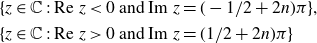 \begin{equation*} \begin{split} \{z\in \mathbb{C} \;:\; \textrm{Re} \; z<0 & \text{ and }\textrm{Im} \; z= (-1/2+2n)\pi \},\\ \{z\in \mathbb{C}\;:\; \textrm{Re} \; z >0 & \text{ and }\textrm{Im} \; z = (1/2+2 n)\pi \} \end{split} \end{equation*}
for all $n \in \mathbb{Z}$
. Thus, each fundamental domain is contained in one of the half-strips
$n \in \mathbb{Z}$
. Thus, each fundamental domain is contained in one of the half-strips
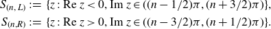 \begin{equation} \begin{split} S_{(n,\,L)}& \;:\!=\; \{z\;:\; \textrm{Re} \; z<0, \textrm{Im} \; z\in ((n-1/2)\pi ,(n+3/2)\pi)\},\\ S_{(n,R)}& \;:\!=\; \{z\;:\; \textrm{Re} \; z>0, \textrm{Im} \; z\in ((n-3/2)\pi,(n+1/2)\pi)\}. \end{split} \end{equation}
For each $(n,\ast)\in \mathbb{Z} \times \{-,+\}$
, we denote by
$(n,\ast)\in \mathbb{Z} \times \{-,+\}$
, we denote by $n_\ast$
the unique fundamental domain contained in
$n_\ast$
the unique fundamental domain contained in $S_{(n, \ast)}$
. Using these fundamental domains, we define the set of external addresses
$S_{(n, \ast)}$
. Using these fundamental domains, we define the set of external addresses $\textrm{Addr}(\,f)$
, and fix the corresponding set of signed external addresses
$\textrm{Addr}(\,f)$
, and fix the corresponding set of signed external addresses $\textrm{Addr}(\,f)_\pm$
; see Definition and Theorem 4.4. In particular, for the curves
$\textrm{Addr}(\,f)_\pm$
; see Definition and Theorem 4.4. In particular, for the curves $\gamma_1$
and
$\gamma_1$
and $\gamma_{-1}$
introduced in Section 5·3, it holds that
$\gamma_{-1}$
introduced in Section 5·3, it holds that $f(\gamma_{-1}) \subset \gamma_1$
,
$f(\gamma_{-1}) \subset \gamma_1$
, $f(\gamma_1)\subset \gamma_1$
,
$f(\gamma_1)\subset \gamma_1$
,
![]() and
and
![]() . Moreover, each of these curves equals two canonical tails with opposite sign, as they do not contain preimages of critical points, see Proposition 5·2. Hence,
. Moreover, each of these curves equals two canonical tails with opposite sign, as they do not contain preimages of critical points, see Proposition 5·2. Hence,
![]() and
and
![]() for both
for both $\ast \in \{-,+\}$
; see Figure 2.
$\ast \in \{-,+\}$
; see Figure 2.
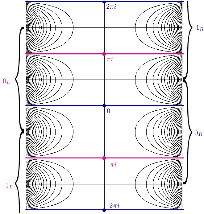
Fig. 2. Partition of the plane into fundamental domains and itinerary components of $f(z)=\cosh(z)$
. Each strip of height
$f(z)=\cosh(z)$
. Each strip of height $\pi$
between two coloured horizontal lines is an itinerary domain. Strips that contain some fundamental domains are indicated by keys. Black horizontal lines are preimages of the imaginary axis, and the rest of curves are the preimages of all horizontal lines.
$\pi$
between two coloured horizontal lines is an itinerary domain. Strips that contain some fundamental domains are indicated by keys. Black horizontal lines are preimages of the imaginary axis, and the rest of curves are the preimages of all horizontal lines.
The dynamical partition from Section will help us determine that no two dynamic rays of f land together. This is because since the boundaries of the elements in $\mathcal{U}$
are ray tails, as we shall see, no other ray tails can cross them. More precisely, in the next proposition, we assign to each curve
$\mathcal{U}$
are ray tails, as we shall see, no other ray tails can cross them. More precisely, in the next proposition, we assign to each curve $\{\overline{\Gamma({\underline s}, \ast)}\}_{({\underline s},\ast)\in \textrm{Addr}(\,f)_\pm}$
a unique element of
$\{\overline{\Gamma({\underline s}, \ast)}\}_{({\underline s},\ast)\in \textrm{Addr}(\,f)_\pm}$
a unique element of $\mathcal{U}$
:
$\mathcal{U}$
:
Proposition 5·5 (Each canonical ray is in the closure of a unique $U\in \mathcal{U}$
). For each
$U\in \mathcal{U}$
). For each $({\underline s}, \ast)\in \textrm{Addr}(\,f)_\pm$
, there exists a unique component
$({\underline s}, \ast)\in \textrm{Addr}(\,f)_\pm$
, there exists a unique component $U\in \mathcal{U}$
such that
$U\in \mathcal{U}$
such that $\overline{\Gamma({\underline s}, \ast)} \subset \overline{U}$
. We denote
$\overline{\Gamma({\underline s}, \ast)} \subset \overline{U}$
. We denote
 \begin{equation*}U({\underline s}, \ast)\;:\!=\; U.\end{equation*}
Proof. Since, as described in Section 5·4, the set X defined in (5·3) consists of four canonical tails that overlap pairwise, and, in addition, f is totally ramified, exactly four canonical tails meet at each critical point of $f^{-1}(X)$
, and their union is a connected component of this set. More precisely, following the analysis in Section 5·4,
$f^{-1}(X)$
, and their union is a connected component of this set. More precisely, following the analysis in Section 5·4, $f^{-1}(\gamma_1)$
is the collection of all the horizontal lines
$f^{-1}(\gamma_1)$
is the collection of all the horizontal lines $\{2\pi K i\mathbb{R}\}_{K \in \mathbb{Z}}$
, that in particular contain the critical points
$\{2\pi K i\mathbb{R}\}_{K \in \mathbb{Z}}$
, that in particular contain the critical points $2\pi K i$
for all
$2\pi K i$
for all $K\in \mathbb{Z}$
. Analogously,
$K\in \mathbb{Z}$
. Analogously, $f^{-1}(\gamma_{-1})$
is the collection of the horizontal lines
$f^{-1}(\gamma_{-1})$
is the collection of the horizontal lines $\{2(K+1)\pi i \mathbb{R}\}_{K \in \mathbb{Z}}$
with critical points at
$\{2(K+1)\pi i \mathbb{R}\}_{K \in \mathbb{Z}}$
with critical points at $2(K+1)\pi i$
for each
$2(K+1)\pi i$
for each $K\in \mathbb{Z}$
. Hence, it follows that for each
$K\in \mathbb{Z}$
. Hence, it follows that for each $K\in \mathbb{Z}$
and
$K\in \mathbb{Z}$
and $\ast\in \{-,+\}$
,
$\ast\in \{-,+\}$
,
We claim that each of the canonical rays displayed in (5·5) belongs to the closure of exactly one component of $\mathcal{U}$
: to see this, let us consider the curves
$\mathcal{U}$
: to see this, let us consider the curves
![]() for some
for some $K\in \mathbb{Z}$
and both
$K\in \mathbb{Z}$
and both $\ast\in \{-,+\}$
. Then, since
$\ast\in \{-,+\}$
. Then, since
![]() is a nested sequence of left-extended canonical tails, see [
Reference Pardo–Simón18
, definition 3·5 and theorem 3·8], and by Proposition 5·2 it can only intersect the boundaries of the elements of
is a nested sequence of left-extended canonical tails, see [
Reference Pardo–Simón18
, definition 3·5 and theorem 3·8], and by Proposition 5·2 it can only intersect the boundaries of the elements of $\mathcal{U}$
in the subcurve
$\mathcal{U}$
in the subcurve $2K\pi i \mathbb{R}^+$
, we conclude that
$2K\pi i \mathbb{R}^+$
, we conclude that
![]() . Similarly,
. Similarly,
![]() , and arguing analogously for the rest of curves in (5·5), the claim follows. Since no other canonical rays apart from those in (5·5) intersect
, and arguing analogously for the rest of curves in (5·5), the claim follows. Since no other canonical rays apart from those in (5·5) intersect $\mathbb{C} \setminus \mathcal{U}$
, each of them must be contained in a unique component U, as stated.
$\mathbb{C} \setminus \mathcal{U}$
, each of them must be contained in a unique component U, as stated.
Definition 5·6 (Itineraries for $f(z)=\cosh(z)$
). For each
$f(z)=\cosh(z)$
). For each $({\underline s}, \ast)\in \textrm{Addr}(\,f)_\pm$
, we define the itinerary of
$({\underline s}, \ast)\in \textrm{Addr}(\,f)_\pm$
, we define the itinerary of $({\underline s}, \ast)$
as the infinite sequence
$({\underline s}, \ast)$
as the infinite sequence
 \begin{equation*}\textrm{itin}({\underline s}, \ast)\;:\!=\; U({\underline s}, \ast) U(\sigma({\underline s}), \ast)U(\sigma^2({\underline s}), \ast)\cdots. \end{equation*}
Observation 5·7 (Itineraries of points). Since for each $({\underline s}, \ast) \in \textrm{Addr}(\,f)_\pm$
,
$({\underline s}, \ast) \in \textrm{Addr}(\,f)_\pm$
, $f(\overline{\Gamma({\underline s}, \ast)})\subset \overline{\Gamma}(\sigma({\underline s}), \ast)$
, if
$f(\overline{\Gamma({\underline s}, \ast)})\subset \overline{\Gamma}(\sigma({\underline s}), \ast)$
, if $z\in \overline{\Gamma({\underline s}, \ast)}$
and
$z\in \overline{\Gamma({\underline s}, \ast)}$
and $\textrm{itin}({\underline s}, \ast)=U_0U_1\cdots$
, then
$\textrm{itin}({\underline s}, \ast)=U_0U_1\cdots$
, then $f^i(z)\subset U_i$
for all
$f^i(z)\subset U_i$
for all $i\geq 0$
.
$i\geq 0$
.
Proposition 5·8 (Dynamic rays of $z \mapsto \cosh(z)$
do not land together). There are no two dynamic rays of
$z \mapsto \cosh(z)$
do not land together). There are no two dynamic rays of $z \mapsto \cosh(z)$
landing together.
$z \mapsto \cosh(z)$
landing together.
Proof. It suffices to show that there are no two canonical rays landing together, since then, by Definition and Theorem 4.4, no two rays would land together. With that aim, let $\Gamma({\underline s}, \ast)$
and
$\Gamma({\underline s}, \ast)$
and $\Gamma(\underline{\tau}, \star)$
be two different canonical rays, that is,
$\Gamma(\underline{\tau}, \star)$
be two different canonical rays, that is, $({\underline s}, \ast)\neq (\underline{\tau}, \star)$
, and let
$({\underline s}, \ast)\neq (\underline{\tau}, \star)$
, and let $p_{({\underline s}, \ast)}$
and
$p_{({\underline s}, \ast)}$
and $p_{(\underline{\tau}, \star)}$
be their respective endpoints. If
$p_{(\underline{\tau}, \star)}$
be their respective endpoints. If $\Gamma({\underline s}, \ast)$
and
$\Gamma({\underline s}, \ast)$
and $\Gamma(\underline{\tau}, \star)$
land together, i.e.,
$\Gamma(\underline{\tau}, \star)$
land together, i.e., $p_{({\underline s}, \ast)}= p_{(\underline{\tau}, \star)}$
, then by Proposition 5·5 and Observation 5·7,
$p_{({\underline s}, \ast)}= p_{(\underline{\tau}, \star)}$
, then by Proposition 5·5 and Observation 5·7, $\textrm{itin}({\underline s}, \ast)=\textrm{itin}(\underline{\tau}, \ast)=U_0U_1\cdots$
. Moreover, for each
$\textrm{itin}({\underline s}, \ast)=\textrm{itin}(\underline{\tau}, \ast)=U_0U_1\cdots$
. Moreover, for each $i\geq 0$
,
$i\geq 0$
, $f^i(p_{({\underline s}, \ast)})=f^i(p_{(\underline{\tau}, \star)})$
must belong to the interior of
$f^i(p_{({\underline s}, \ast)})=f^i(p_{(\underline{\tau}, \star)})$
must belong to the interior of $U_i$
, since by 5.4, the boundaries of the elements of
$U_i$
, since by 5.4, the boundaries of the elements of $\mathcal{U}$
are formed by canonical tails that are contained in dynamic rays. For the same reason,
$\mathcal{U}$
are formed by canonical tails that are contained in dynamic rays. For the same reason, $i\mathbb{R}^+$
and
$i\mathbb{R}^+$
and $f^{-1}(i\mathbb{R}^+)$
do not contain any endpoints of dynamic rays, as they are formed by pieces of ray tails; see Section for more details. Then, for each
$f^{-1}(i\mathbb{R}^+)$
do not contain any endpoints of dynamic rays, as they are formed by pieces of ray tails; see Section for more details. Then, for each $i\geq 0$
,
$i\geq 0$
, $f^i(p_{({\underline s}, \ast)})=f^i(p_{(\underline{\tau}, \star)})$
belongs to a half-strip of the form
$f^i(p_{({\underline s}, \ast)})=f^i(p_{(\underline{\tau}, \star)})$
belongs to a half-strip of the form
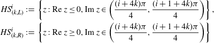 \begin{equation} \begin{split} HS^i_{(k,L)}&\;:\!=\; \left\{ z\;:\; \textrm{Re} \; z\leq 0, \textrm{Im} \; z\in \left(\frac{(i+4k)\pi}{4} ,\frac{(i+1+4k)\pi}{4}\right) \right\},\\ HS^i_{(k,R)}&\;:\!=\; \left\{ z\;:\; \textrm{Re} \; z\geq 0, \textrm{Im} \; z\in \left(\frac{(i+4k)\pi}{4} ,\frac{(i+1+4k)\pi}{4}\right) \right\} \end{split} \end{equation}
for some $k\in \mathbb{Z}$
and
$k\in \mathbb{Z}$
and $0\leq i \leq 3$
. However, each of the half-strips in (5·6) intersects a single fundamental domain, see (5·4) and Figure 2, which contradicts
$0\leq i \leq 3$
. However, each of the half-strips in (5·6) intersects a single fundamental domain, see (5·4) and Figure 2, which contradicts $({\underline s}, \ast)\neq (\underline{\tau}, \star)$
.
$({\underline s}, \ast)\neq (\underline{\tau}, \star)$
.
Finally, we provide a combinatorial description of the overlaps that occur between canonical rays in terms of their signed addresses, which by Observation 5·1 and Proposition 5·8 suffices to describe the equivalence classes in $J(\mathcal{F})/ {\sim}$
.
$J(\mathcal{F})/ {\sim}$
.
5·9 (Overlapping of canonical tails for $ z \mapsto \cosh(z)$
). Recall that by Proposition 5·2, for all
$ z \mapsto \cosh(z)$
). Recall that by Proposition 5·2, for all $({\underline s}, \ast)\in \textrm{Addr}(\,f)_\pm$
such that
$({\underline s}, \ast)\in \textrm{Addr}(\,f)_\pm$
such that $\Gamma({\underline s}, \ast) \cap \textrm{Orb}^-(\textrm{Crit} (\,f))=\emptyset$
,
$\Gamma({\underline s}, \ast) \cap \textrm{Orb}^-(\textrm{Crit} (\,f))=\emptyset$
, $\Gamma({\underline s}, -)=\Gamma({\underline s}, +).$
Hence, all other overlap occurs between the preimages of the canonical tails that contain
$\Gamma({\underline s}, -)=\Gamma({\underline s}, +).$
Hence, all other overlap occurs between the preimages of the canonical tails that contain $\textrm{Crit}(\,f)$
. Recall from Section and that
$\textrm{Crit}(\,f)$
. Recall from Section and that $\textrm{Crit}(\,f)=\{\pi i K\;:\;K \in \mathbb{Z}\}$
, and each critical point belongs exactly to four canonical rays. Namely, we saw in (5·5) that
$\textrm{Crit}(\,f)=\{\pi i K\;:\;K \in \mathbb{Z}\}$
, and each critical point belongs exactly to four canonical rays. Namely, we saw in (5·5) that
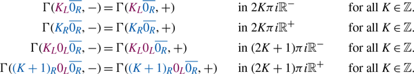
Further identifications between the canonical rays above occur at the connected components of $f^{-1}([0,1])$
and
$f^{-1}([0,1])$
and $f^{-1}([-1,0])$
. More precisely, if for each
$f^{-1}([-1,0])$
. More precisely, if for each $\pm\in \{-,+\}$
we denote
$\pm\in \{-,+\}$
we denote
 \begin{equation*}V_K(\pm)\;:\!=\; \left\{z \in \mathbb{C}\;:\; \textrm{Re} \; z=0 \text{ and } \textrm{Im} \; z\in [K\pi i,(K \pm 1/2)\pi i ]\right\},\end{equation*}
then we have the following identifications:
where $\mp=+$
when
$\mp=+$
when $\pm=-$
, and
$\pm=-$
, and $\mp=-$
when
$\mp=-$
when $\pm=+$
; see Figure 3. By Proposition 5·2, any further overlap between canonical rays occur at preimages of the overlap already stated. More specifically, since we have already described all overlap occurring at the boundaries of the elements in
$\pm=+$
; see Figure 3. By Proposition 5·2, any further overlap between canonical rays occur at preimages of the overlap already stated. More specifically, since we have already described all overlap occurring at the boundaries of the elements in $\mathcal{U}$
, all remaining ones must occur between canonical rays whose itinerary agrees on the first N-th elements and that are mapped under
$\mathcal{U}$
, all remaining ones must occur between canonical rays whose itinerary agrees on the first N-th elements and that are mapped under $f^N$
to the coordinate axes for some
$f^N$
to the coordinate axes for some $N\in \mathbb{N}$
. Given the geometry of the fundamental domains, in particular contained in half-strips of height
$N\in \mathbb{N}$
. Given the geometry of the fundamental domains, in particular contained in half-strips of height $\pi$
, see (5·4) and Figure 2, providing the identifications at the preimages of the positive imaginary axis allows us to express identifications solely using external addresses. This is because any further identifications must occur at the intersection of a fundamental domain with a component of
$\pi$
, see (5·4) and Figure 2, providing the identifications at the preimages of the positive imaginary axis allows us to express identifications solely using external addresses. This is because any further identifications must occur at the intersection of a fundamental domain with a component of $\mathcal{U}$
, and hence, the corresponding first entries on the signed addresses of rays that overlap are the same. More specifically, for each
$\mathcal{U}$
, and hence, the corresponding first entries on the signed addresses of rays that overlap are the same. More specifically, for each $\pm\in \{-,+\}$
, let us denote
$\pm\in \{-,+\}$
, let us denote
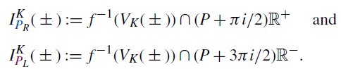
Then, for all $K \in \mathbb{Z}^+ \text{ and } P\in \mathbb{Z}$
,
$K \in \mathbb{Z}^+ \text{ and } P\in \mathbb{Z}$
,
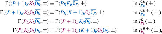
where $\mp=+$
when
$\mp=+$
when $\pm=-$
, and
$\pm=-$
, and $\mp=-$
when
$\mp=-$
when $\pm=+$
; see Figure 3. Moreover, for all other canonical rays, if
$\pm=+$
; see Figure 3. Moreover, for all other canonical rays, if $\delta$
is some bounded curve in J(f), then
$\delta$
is some bounded curve in J(f), then
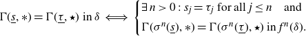 \begin{equation} \Gamma({\underline s}, \ast) =\Gamma(\underline{\tau}, \star) \text { in } \delta \iff \left\{\begin{array}{@{}l@{\quad}l@{}} \exists \, n>0 \;:\; s_j=\tau_j \text{ for all } j\leq n \quad \text{and}\\[5pt] \Gamma(\sigma^n({\underline s}), \ast) = \Gamma(\sigma^n(\underline{\tau}), \star) \text { in } f^n(\delta). \end{array}\right. \end{equation}
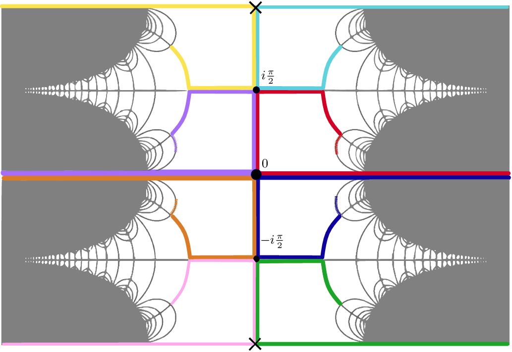
Fig. 3. Some canonical tails in the Julia set of the map $z \mapsto \cosh(z)$
that belong to canonical rays. Colour code: the red tail is in
$z \mapsto \cosh(z)$
that belong to canonical rays. Colour code: the red tail is in
![]() , the purple in
, the purple in
![]() , the orange in
, the orange in
![]() and the dark blue one in
and the dark blue one in
![]() . Then, the light blue tail is in
. Then, the light blue tail is in
![]() , the yellow one in
, the yellow one in
![]() , the green is in
, the green is in
![]() and the pink is in
and the pink is in
![]() .
.
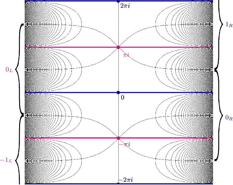
Fig. 4. Partition of the plane into fundamental domains and itinerary components for $z \mapsto \cosh^2(z)$
. Each strip of height
$z \mapsto \cosh^2(z)$
. Each strip of height $\pi$
between two coloured lines is an itinerary domain. Some fundamental domains are indicated by keys. Also displayed are the first (coloured lines and imaginary axis), second (other curves that meet at
$\pi$
between two coloured lines is an itinerary domain. Some fundamental domains are indicated by keys. Also displayed are the first (coloured lines and imaginary axis), second (other curves that meet at $\{K\pi i\;:\;K\in \mathbb{Z}\}$
) and third (rest of curves) iterated preimages of the real line.
$\{K\pi i\;:\;K\in \mathbb{Z}\}$
) and third (rest of curves) iterated preimages of the real line.
We have now provided a combinatorial description of all overlappings occurring between canonical rays of $z \mapsto \cosh(z)$
, as well as determined that no two of its dynamic rays land together. Hence, we have concluded our analysis.
$z \mapsto \cosh(z)$
, as well as determined that no two of its dynamic rays land together. Hence, we have concluded our analysis.
Example 5·10 (Overlapping for the map $z \mapsto \cosh^2(z)$
). Seeking an example where a critical value is mapped to another critical value, we consider the function
$z \mapsto \cosh^2(z)$
). Seeking an example where a critical value is mapped to another critical value, we consider the function
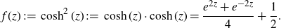 \begin{equation*}f(z)\;:\!=\; \cosh^2 (z)\;:\!=\; \cosh (z) \cdot \cosh (z) =\dfrac{e^{2z}+ e^{-2z}}{4}+ \dfrac{1}{2}.\end{equation*}
Even if, strictly speaking, this function is not in the cosine family, it is in the same parameter space, since f is conjugate to $({e}/{2})e^w+ ({e^{-1}}/{2})e^{-w}$
via
$({e}/{2})e^w+ ({e^{-1}}/{2})e^{-w}$
via $z \mapsto 2z-1$
. The dynamics of f have already been explored, namely in [
Reference Rippon and Stallard26
], where it is shown that I(f) (and in fact its fast escaping set) is connected. The function f is
$z \mapsto 2z-1$
. The dynamics of f have already been explored, namely in [
Reference Rippon and Stallard26
], where it is shown that I(f) (and in fact its fast escaping set) is connected. The function f is $\pi i$
-periodic, and
$\pi i$
-periodic, and $S(\,f)= \textrm{CV}(\,f)=\{0,1\}$
, with
$S(\,f)= \textrm{CV}(\,f)=\{0,1\}$
, with $f(0)=1 \in I(\,f)$
and
$f(0)=1 \in I(\,f)$
and ${Orb}^+(1) \subset \mathbb{R}^+$
. The critical points of f are
${Orb}^+(1) \subset \mathbb{R}^+$
. The critical points of f are $f^{-1}(1)=\{K\pi i\;:\;K \in \mathbb{Z} \}$
and
$f^{-1}(1)=\{K\pi i\;:\;K \in \mathbb{Z} \}$
and $f^{-1}(0)=\{(K+1/2)\pi i : K \in \mathbb{Z} \}.$
As for the map
$f^{-1}(0)=\{(K+1/2)\pi i : K \in \mathbb{Z} \}.$
As for the map $z \mapsto \cosh(z)$
, we can join the critical values to infinity using the ray tails
$z \mapsto \cosh(z)$
, we can join the critical values to infinity using the ray tails $\gamma_1\;:\!=\; \mathbb{R} \setminus (-\infty, 1)$
and
$\gamma_1\;:\!=\; \mathbb{R} \setminus (-\infty, 1)$
and $\gamma_{0}\;:\!=\; \mathbb{R} \setminus (0, \infty)$
. We define a dynamical partition for f as the union of the connected components of
$\gamma_{0}\;:\!=\; \mathbb{R} \setminus (0, \infty)$
. We define a dynamical partition for f as the union of the connected components of $\mathbb{C} \setminus f^{-1}(\gamma_0\cup \gamma_1)$
, which are horizontal half-strips of
$\mathbb{C} \setminus f^{-1}(\gamma_0\cup \gamma_1)$
, which are horizontal half-strips of $\pi/2$
-height that we call itinerary components; see Figure 4. By choosing a bounded domain D containing [0,
Reference Aarts and Oversteegen1
] and
$\pi/2$
-height that we call itinerary components; see Figure 4. By choosing a bounded domain D containing [0,
Reference Aarts and Oversteegen1
] and $\delta\;:\!=\; i\mathbb{R}^+\setminus D$
, we can define fundamental domains for f as the connected components of
$\delta\;:\!=\; i\mathbb{R}^+\setminus D$
, we can define fundamental domains for f as the connected components of $f^{-1}(\mathbb{C}\setminus (\overline{D}\cup \delta))$
. In particular, we label as
$f^{-1}(\mathbb{C}\setminus (\overline{D}\cup \delta))$
. In particular, we label as
the component that contains an unbounded subset of $\mathbb{R}^+$
, and as
$\mathbb{R}^+$
, and as
the component that contains an unbounded subcurve of $\mathbb{R}^-$
. Additionally, we label as
$\mathbb{R}^-$
. Additionally, we label as
and
their respective $K\pi i$
-translates; see Figure 4. With this notation, the following identifications between canonical rays occur:
$K\pi i$
-translates; see Figure 4. With this notation, the following identifications between canonical rays occur:
The main difference between the overlap on the canonical rays of $z \mapsto\cosh(z)$
and the overlap on those of f, is that since the critical points in
$z \mapsto\cosh(z)$
and the overlap on those of f, is that since the critical points in $f^{-1}(0)$
are mapped to a critical point, each of them belongs to eight canonical tails rather than to four, and moreover, both singular values belong to the canonical rays
$f^{-1}(0)$
are mapped to a critical point, each of them belongs to eight canonical tails rather than to four, and moreover, both singular values belong to the canonical rays
for both $\ast\in \{-,+\}$
. Compare Figures 3 and 5. Then, we further have the identifications
$\ast\in \{-,+\}$
. Compare Figures 3 and 5. Then, we further have the identifications
where $\mp=+$
when
$\mp=+$
when $\pm=-$
, and
$\pm=-$
, and $\mp=-$
when
$\mp=-$
when $\pm=+$
. If for each
$\pm=+$
. If for each $\pm \in \{-,+\}$
and
$\pm \in \{-,+\}$
and $K\in \mathbb{Z}$
we let
$K\in \mathbb{Z}$
we let
then for all $K \in \mathbb{Z}^+$
and
$K \in \mathbb{Z}^+$
and $P\in \mathbb{Z}$
,
$P\in \mathbb{Z}$
,
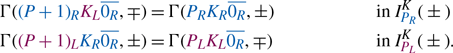
Any further identifications between canonical rays occur within the intersection of a fundamental domain and an itinerary domain, and hence can be expressed using (5·7). Moreover, arguing as for $z \mapsto \cosh(z)$
, no two dynamic rays of
$z \mapsto \cosh(z)$
, no two dynamic rays of $z \mapsto \cosh^2(z)$
land together, see the proof of Proposition 5·8.
$z \mapsto \cosh^2(z)$
land together, see the proof of Proposition 5·8.
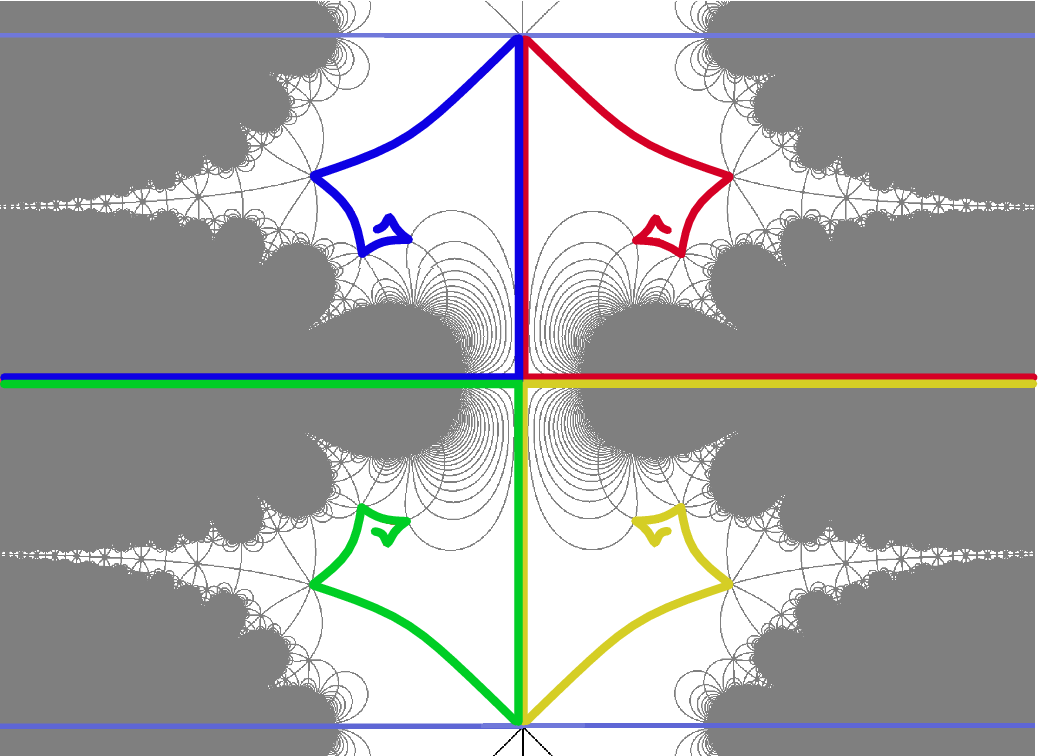
Fig. 5. Picture showing four canonical tails of $z \mapsto \cosh^2(z)$
that contain the critical point 0. These belong to the canonical rays
$z \mapsto \cosh^2(z)$
that contain the critical point 0. These belong to the canonical rays
![]() (in blue),
(in blue),
![]() (in red),
(in red),
![]() (in green) and
(in green) and
![]() (in yellow).
(in yellow).
Appendix A. Itineraries and rays landing together
This section concerns certain sps maps in $\mathcal{B}$
that have dynamic rays on their Julia sets. Namely, in [
Reference Pardo–Simón19
], the following class is introduced:
$\mathcal{B}$
that have dynamic rays on their Julia sets. Namely, in [
Reference Pardo–Simón19
], the following class is introduced:
Definition A1. We say that $f \in \mathcal{B}$
belongs to the class
$f \in \mathcal{B}$
belongs to the class $\mathcal{CB}$
if
$\mathcal{CB}$
if $J(\lambda f)$
is a Cantor bouquet for some
$J(\lambda f)$
is a Cantor bouquet for some $\vert \lambda \vert$
sufficiently small. It follows from [
Reference Pardo–Simón19
, theorem 1·4] that some iterate of each escaping point of any function
$\vert \lambda \vert$
sufficiently small. It follows from [
Reference Pardo–Simón19
, theorem 1·4] that some iterate of each escaping point of any function $f\in \mathcal{CB}$
can be joined to infinity by a dynamic ray, and that the concept of canonical rays can be extended to maps in this class. Moreover, the class
$f\in \mathcal{CB}$
can be joined to infinity by a dynamic ray, and that the concept of canonical rays can be extended to maps in this class. Moreover, the class $\mathcal{CB}$
includes all finite compositions of class
$\mathcal{CB}$
includes all finite compositions of class $\mathcal{B}$
functions of finite order, and in particular, all cosine maps; see [
Reference Pardo–Simón19
, proposition 6].
$\mathcal{B}$
functions of finite order, and in particular, all cosine maps; see [
Reference Pardo–Simón19
, proposition 6].
In this section, we extend the concept of itineraries introduced in Section 5 for the functions $z\mapsto \cosh(z)$
and
$z\mapsto \cosh(z)$
and $z \mapsto \cosh^2(z)$
to all strongly postcritically separated functions in class
$z \mapsto \cosh^2(z)$
to all strongly postcritically separated functions in class $\mathcal{CB}$
, and use it to provide some combinatorial criteria for their canonical rays landing together in Theorem A12. This idea, that comes from polynomial dynamics, has already been used in the study of the exponential and cosine families; see for example [
Reference Rempe22
,
Reference Schleicher29
]. Moreover, a more general and systematic definition of itineraries for geometrically finite functions can be found in [
Reference Mihaljević–Brandt13
, chapter 5]. We say that
$\mathcal{CB}$
, and use it to provide some combinatorial criteria for their canonical rays landing together in Theorem A12. This idea, that comes from polynomial dynamics, has already been used in the study of the exponential and cosine families; see for example [
Reference Rempe22
,
Reference Schleicher29
]. Moreover, a more general and systematic definition of itineraries for geometrically finite functions can be found in [
Reference Mihaljević–Brandt13
, chapter 5]. We say that $f\in \mathcal{B}$
is geometrically finite if
$f\in \mathcal{B}$
is geometrically finite if $S(\,f)\cap F(\,f)$
is compact and
$S(\,f)\cap F(\,f)$
is compact and $P_J$
is finite. In particular, only attracting and parabolic basins can occur as Fatou components for maps in this class; [
Reference Mihaljević–Brandt14
, proposition 2·5]. Since for strongly postcritically separated functions in class
$P_J$
is finite. In particular, only attracting and parabolic basins can occur as Fatou components for maps in this class; [
Reference Mihaljević–Brandt14
, proposition 2·5]. Since for strongly postcritically separated functions in class $\mathcal{B}$
the only possible Fatou components are attracting basins, [
Reference Pardo–Simón20
, lemma 2·6], some of the definitions in [
Reference Mihaljević–Brandt13
, chapter 5] will adapt to our setting.
$\mathcal{B}$
the only possible Fatou components are attracting basins, [
Reference Pardo–Simón20
, lemma 2·6], some of the definitions in [
Reference Mihaljević–Brandt13
, chapter 5] will adapt to our setting.
For the rest of the section, let us fix $f\in \mathcal{CB}$
and strongly postcritically separated. We note that the definition of signed addresses that we provided for sps cosine maps in (4·2), as well as that of canonical rays, extends to all sps maps in
$f\in \mathcal{CB}$
and strongly postcritically separated. We note that the definition of signed addresses that we provided for sps cosine maps in (4·2), as well as that of canonical rays, extends to all sps maps in $\mathcal{CB}$
, see [
Reference Pardo–Simón18
, section 3]. Let us also fix
$\mathcal{CB}$
, see [
Reference Pardo–Simón18
, section 3]. Let us also fix $g\;:\!=\; \lambda f$
of disjoint type for some
$g\;:\!=\; \lambda f$
of disjoint type for some $\lambda \in \mathbb{C}^\ast$
, and let
$\lambda \in \mathbb{C}^\ast$
, and let $J(g)_\pm\;:\!=\; J(g)\times \{-,+\}.$
For each
$J(g)_\pm\;:\!=\; J(g)\times \{-,+\}.$
For each ${\underline s}\in \textrm{Addr}(g)$
and
${\underline s}\in \textrm{Addr}(g)$
and $\ast \in \{-,+\}$
, denote
$\ast \in \{-,+\}$
, denote $J_{({\underline s}, \ast)}\;:\!=\; J_{\underline s}\times \{\ast\}$
. Let us define the function
$J_{({\underline s}, \ast)}\;:\!=\; J_{\underline s}\times \{\ast\}$
. Let us define the function $\tilde{g}\colon J(g)_\pm\rightarrow J(g)_\pm$
by
$\tilde{g}\colon J(g)_\pm\rightarrow J(g)_\pm$
by $\tilde{g}(z, \ast)\;:\!=\;(g(z), \ast).$
Then, [
Reference Pardo–Simón21
, theorem 6·5] states that there exists a continuous surjective map
$\tilde{g}(z, \ast)\;:\!=\;(g(z), \ast).$
Then, [
Reference Pardo–Simón21
, theorem 6·5] states that there exists a continuous surjective map
 \begin{equation}\varphi\;:\; J(g)_\pm \to J(\,f)\end{equation}
such that
 \begin{equation} f\circ\varphi = \varphi\circ \tilde{g}.\end{equation}
Moreover, for each $({\underline s}, \ast) \in \textrm{Addr}(g)_\pm$
,
$({\underline s}, \ast) \in \textrm{Addr}(g)_\pm$
, $\varphi \colon J_{({\underline s}, \ast)} \rightarrow \overline{\Gamma({\underline s}, \ast)}$
is a bijection and
$\varphi \colon J_{({\underline s}, \ast)} \rightarrow \overline{\Gamma({\underline s}, \ast)}$
is a bijection and $\overline{\Gamma({\underline s}, \ast)}$
is a canonical ray together with its endpoint. In particular,
$\overline{\Gamma({\underline s}, \ast)}$
is a canonical ray together with its endpoint. In particular, $\varphi$
establishes a one-to-one correspondence between
$\varphi$
establishes a one-to-one correspondence between $\textrm{Addr}(g)_\pm$
and
$\textrm{Addr}(g)_\pm$
and $\textrm{Addr}(\,f)_\pm$
; see [
Reference Pardo–Simón21
, observation 6·6].
$\textrm{Addr}(\,f)_\pm$
; see [
Reference Pardo–Simón21
, observation 6·6].
Our first goal is to define a forward-invariant closed set $K \Supset P(\,f)$
such that
$K \Supset P(\,f)$
such that $J(\,f)\subset \overline{\mathbb{C} \setminus K}$
and so that each connected component of
$J(\,f)\subset \overline{\mathbb{C} \setminus K}$
and so that each connected component of $\mathbb{C} \setminus K$
is simply-connected. We will then define itineraries for f using such components. More specifically, we will define K as a union of two sets
$\mathbb{C} \setminus K$
is simply-connected. We will then define itineraries for f using such components. More specifically, we will define K as a union of two sets $K_J$
and
$K_J$
and $K_F$
, the first consisting of the union of all canonical rays whose endpoints are in
$K_F$
, the first consisting of the union of all canonical rays whose endpoints are in $P_J$
, and the second comprising all points in
$P_J$
, and the second comprising all points in $P_F$
. Recall from Definition 4·3 that E(f) denotes the set of endpoints of dynamic rays of f.
$P_F$
. Recall from Definition 4·3 that E(f) denotes the set of endpoints of dynamic rays of f.
Proposition A2 (Set of rays sharing their endpoint is closed). For each $z\in E(\,f)$
, denote by
$z\in E(\,f)$
, denote by $\mathcal{R}(z)$
the set of canonical rays that land at z. Then,
$\mathcal{R}(z)$
the set of canonical rays that land at z. Then, $\overline{\mathcal{R}}(z)\;:\!=\;\mathcal{R}(z) \cup \{z\}$
is closed.
$\overline{\mathcal{R}}(z)\;:\!=\;\mathcal{R}(z) \cup \{z\}$
is closed.
Proof. Let $\varphi$
be the function from (A1). Since
$\varphi$
be the function from (A1). Since $\varphi$
is continuous,
$\varphi$
is continuous, $\varphi^{-1}(z)$
is a closed set of
$\varphi^{-1}(z)$
is a closed set of $J(g)_\pm$
, being each connected component of
$J(g)_\pm$
, being each connected component of $\varphi^{-1}(z)$
the endpoint
$\varphi^{-1}(z)$
the endpoint $(e_{\underline s}, \ast)$
of a set
$(e_{\underline s}, \ast)$
of a set $J_{(s, \ast)}\subset J(g)_\pm$
. Let
$J_{(s, \ast)}\subset J(g)_\pm$
. Let $J(g)_\pm \cup\{\widetilde{\infty}\}$
be the one-point compactification of
$J(g)_\pm \cup\{\widetilde{\infty}\}$
be the one-point compactification of $J(g)_\pm$
; see [
Reference Pardo–Simón21
, lemma 5·8]. Then, the set
$J(g)_\pm$
; see [
Reference Pardo–Simón21
, lemma 5·8]. Then, the set $\mathcal{P}\;:\!=\; \{J_{({\underline s}, \ast)} \colon (e_{\underline s}, \ast)\in \varphi^{-1}(z) \}\cup \{\widetilde{\infty}\}$
is compact. We can extend
$\mathcal{P}\;:\!=\; \{J_{({\underline s}, \ast)} \colon (e_{\underline s}, \ast)\in \varphi^{-1}(z) \}\cup \{\widetilde{\infty}\}$
is compact. We can extend $\varphi$
to a continuous map
$\varphi$
to a continuous map $\varphi'\;:\;J(g)_{\pm} \cup \lbrace \widetilde{\infty} \rbrace \rightarrow J(\,f) \cup \lbrace \infty \rbrace$
by defining
$\varphi'\;:\;J(g)_{\pm} \cup \lbrace \widetilde{\infty} \rbrace \rightarrow J(\,f) \cup \lbrace \infty \rbrace$
by defining $\varphi'(\widetilde{\infty})=\infty$
, see the proof of [
Reference Pardo–Simón21
, theorem 6·5]. By continuity of
$\varphi'(\widetilde{\infty})=\infty$
, see the proof of [
Reference Pardo–Simón21
, theorem 6·5]. By continuity of $\varphi'$
, we have that
$\varphi'$
, we have that $\varphi'\left(\mathcal{P} \right)$
is compact. By definition of
$\varphi'\left(\mathcal{P} \right)$
is compact. By definition of $\varphi'$
, it must be the case that
$\varphi'$
, it must be the case that $\varphi'(\mathcal{P}\setminus \{\widetilde{\infty}\})=\varphi(\mathcal{P}\setminus \{\widetilde{\infty}\})$
, and by removing
$\varphi'(\mathcal{P}\setminus \{\widetilde{\infty}\})=\varphi(\mathcal{P}\setminus \{\widetilde{\infty}\})$
, and by removing $\lbrace\infty\rbrace$
from the codomain of
$\lbrace\infty\rbrace$
from the codomain of $\varphi'$
, we can conclude that
$\varphi'$
, we can conclude that $\varphi(\mathcal{P}\setminus \{\widetilde{\infty}\})=\overline{\mathcal{R}}(z)$
is (relatively) closed in J(f) with respect to the original topologies.
$\varphi(\mathcal{P}\setminus \{\widetilde{\infty}\})=\overline{\mathcal{R}}(z)$
is (relatively) closed in J(f) with respect to the original topologies.
A3 (Definition of the set $K_J$
). Denote
$K_J$
). Denote
 \begin{equation} K_J\;:\!=\; \bigcup_{z\in P_J \cap E(\,f)} \overline{\mathcal{R}}(z), \end{equation}
and observe that by Proposition A2 and since $P_J$
is discrete,
$P_J$
is discrete, $K_J$
is closed.
$K_J$
is closed.
In addition, we wish to include in K the compact set $P_F$
. Note that
$P_F$
. Note that $\mathbb{C} \setminus P_F$
is open but not necessarily simply-connected. The idea is to remove a full set
$\mathbb{C} \setminus P_F$
is open but not necessarily simply-connected. The idea is to remove a full set $K_F$
such that
$K_F$
such that $F(\,f) \supset K_F \supset P_F$
, together with a collection of curves that connect each connected component of
$F(\,f) \supset K_F \supset P_F$
, together with a collection of curves that connect each connected component of $K_F$
to infinity. A piece of any such curve will be a dynamic ray, and the other piece will be a preperiodic simple curve inside an attracting basin of F(f). For each attracting periodic point
$K_F$
to infinity. A piece of any such curve will be a dynamic ray, and the other piece will be a preperiodic simple curve inside an attracting basin of F(f). For each attracting periodic point $z_0 \in F(\,f)$
,
$z_0 \in F(\,f)$
, $\mathcal{A}^\ast(z_0)$
denotes the immediate attracting basin of
$\mathcal{A}^\ast(z_0)$
denotes the immediate attracting basin of $z_0$
.
$z_0$
.
Definition A4 (Attracting periodic rays [
Reference Mihaljević–Brandt13
, definition 5·2]). Let f be a transcendental entire function and let $z_0$
be an attracting periodic point of f of period n. A simple curve
$z_0$
be an attracting periodic point of f of period n. A simple curve $\alpha \colon (0,\infty) \rightarrow \mathcal{A}^\ast(z_0)$
is called an attracting periodic ray of f at
$\alpha \colon (0,\infty) \rightarrow \mathcal{A}^\ast(z_0)$
is called an attracting periodic ray of f at $z_0$
(of period n) if
$z_0$
(of period n) if
-
(i)
$f^n(\alpha(t)) = \alpha(2t)$
, -
(ii)
$\lim_{t\rightarrow \infty} \alpha(t) = z_0,$
-
(iii)
$\lim_{t\rightarrow 0} \alpha(t) = w$
, where
$w \in \partial \mathcal{A}^\ast(z_0)$
is a periodic point of f of period
$d\vert n$
.


Observation A5 (Images of attracting rays are attracting rays). If $\alpha$
is an attracting periodic ray of f at
$\alpha$
is an attracting periodic ray of f at $z_0$
, then
$z_0$
, then $f(\alpha)$
is an attracting periodic ray of f at
$f(\alpha)$
is an attracting periodic ray of f at $f(z_0)$
. Furthermore, if f is strongly postcritically separated, by [
Reference Pardo–Simón20
, lemma 2·6],
$f(z_0)$
. Furthermore, if f is strongly postcritically separated, by [
Reference Pardo–Simón20
, lemma 2·6], $w=\lim_{t\rightarrow 0} \alpha(t)$
must be a repelling periodic point of f. The next proposition tells us that we can find at least one attracting periodic ray for every attracting periodic point that also contains a prescribed point belonging to its immediate basin of attraction. This result is a version of [
Reference Mihaljević–Brandt13
, proposition 5·3] stated for our class of maps. Since the proof is exactly the same as for geometrically finite maps, we omit it.
$w=\lim_{t\rightarrow 0} \alpha(t)$
must be a repelling periodic point of f. The next proposition tells us that we can find at least one attracting periodic ray for every attracting periodic point that also contains a prescribed point belonging to its immediate basin of attraction. This result is a version of [
Reference Mihaljević–Brandt13
, proposition 5·3] stated for our class of maps. Since the proof is exactly the same as for geometrically finite maps, we omit it.
Proposition A6 (Attracting rays with prescribed points). Let $f\in \mathcal{B}$
be strongly postcritically separated and let
$f\in \mathcal{B}$
be strongly postcritically separated and let $z_0$
be an attracting periodic point of f. Then, for any point
$z_0$
be an attracting periodic point of f. Then, for any point $\xi$
that belongs to the unbounded component of
$\xi$
that belongs to the unbounded component of $\mathcal{A}^\ast(z_0) \setminus P(\,f)$
, there exists an attracting periodic ray of f at
$\mathcal{A}^\ast(z_0) \setminus P(\,f)$
, there exists an attracting periodic ray of f at $z_0$
in
$z_0$
in $\mathcal{A}^\ast(z_0) \setminus P(\,f) $
that contains
$\mathcal{A}^\ast(z_0) \setminus P(\,f) $
that contains $\xi$
.
$\xi$
.
Our aim goal is to define $K_F$
by enclosing
$K_F$
by enclosing $P_F$
with a finite number of connected sets. Each of them will consist of a bounded domain in F(f), together with (a preimage of) an attracting periodic ray, that either has an endpoint at infinity or at a repelling periodic point p. In the latter case, we will include
$P_F$
with a finite number of connected sets. Each of them will consist of a bounded domain in F(f), together with (a preimage of) an attracting periodic ray, that either has an endpoint at infinity or at a repelling periodic point p. In the latter case, we will include $\overline{\mathcal{R}}(p)$
in
$\overline{\mathcal{R}}(p)$
in $K_F$
. We now formalise these ideas following the approach in [
Reference Mihaljević–Brandt13
, definition and proposition 5·4]:
$K_F$
. We now formalise these ideas following the approach in [
Reference Mihaljević–Brandt13
, definition and proposition 5·4]:
A7 (Definition of the set $K_F$
). Since
$K_F$
). Since $P_F$
is compact, there exists a finite collection
$P_F$
is compact, there exists a finite collection $\{A_i\}^n_{i=1}$
of connected components of F(f) such that
$\{A_i\}^n_{i=1}$
of connected components of F(f) such that $\bigcup^n_{i=1}A_i \supset P_F$
. We can assume that
$\bigcup^n_{i=1}A_i \supset P_F$
. We can assume that $\{A_i\}^n_{i=1}$
is minimal in the sense that
$\{A_i\}^n_{i=1}$
is minimal in the sense that $P_F \cap A_i \neq \emptyset$
for all
$P_F \cap A_i \neq \emptyset$
for all $1\leq i\leq n$
. We moreover can assume without loss of generality that f has only one attracting cycle, since otherwise the same argument applies to each cycle. Let
$1\leq i\leq n$
. We moreover can assume without loss of generality that f has only one attracting cycle, since otherwise the same argument applies to each cycle. Let $\{z_1,\ldots, z_m\}$
be this attracting cycle and let
$\{z_1,\ldots, z_m\}$
be this attracting cycle and let $\{A_i\}^m_{i=1}$
be the corresponding immediate basins, labelled so that
$\{A_i\}^m_{i=1}$
be the corresponding immediate basins, labelled so that $A_i \ni z_i$
for all
$A_i \ni z_i$
for all $1\leq i\leq m$
, and so that
$1\leq i\leq m$
, and so that $f(A_j)\subset A_{j-1}$
for all
$f(A_j)\subset A_{j-1}$
for all $2\leq j\leq n$
. Let us pick any point
$2\leq j\leq n$
. Let us pick any point $z^\ast \in A_n$
so that
$z^\ast \in A_n$
so that $f^j(z^\ast)$
does not belong to P(f) for every
$f^j(z^\ast)$
does not belong to P(f) for every $0\leq j\leq n-m$
. We can find a collection of n bounded Jordan domains
$0\leq j\leq n-m$
. We can find a collection of n bounded Jordan domains $\{J_i\}^n_{i=1}$
such that
$\{J_i\}^n_{i=1}$
such that $J_i \subset A_i$
,
$J_i \subset A_i$
, $J \;:\!=\; \bigcup^n_{i=1} J_i \supset (P_F \cup \textrm{Orb}^+(z^\ast))$
and
$J \;:\!=\; \bigcup^n_{i=1} J_i \supset (P_F \cup \textrm{Orb}^+(z^\ast))$
and $f(J)\Subset J \Subset F(\,f)$
, see [
Reference Mihaljević–Brandt13
, proposition 3·1]. Let
$f(J)\Subset J \Subset F(\,f)$
, see [
Reference Mihaljević–Brandt13
, proposition 3·1]. Let $\xi \;:\!=\; f^{n-m}(z^\ast) \in J_m \setminus P_F$
. By Proposition A6, there exists an attracting periodic ray
$\xi \;:\!=\; f^{n-m}(z^\ast) \in J_m \setminus P_F$
. By Proposition A6, there exists an attracting periodic ray $\alpha_m$
at
$\alpha_m$
at $z_m \in J_m$
that contains
$z_m \in J_m$
that contains $\xi$
. For each
$\xi$
. For each $1 \leq i < m$
, we denote the iterated forward image of
$1 \leq i < m$
, we denote the iterated forward image of $\alpha_m$
by
$\alpha_m$
by $\alpha_i \;:\!=\; f^{m-i}(\alpha_m)$
, which by Observation A5 is an attracting periodic ray at
$\alpha_i \;:\!=\; f^{m-i}(\alpha_m)$
, which by Observation A5 is an attracting periodic ray at $z_i$
. Note that it might occur that
$z_i$
. Note that it might occur that $\lim_{t \rightarrow 0} \alpha_i(t) = \lim_{t \rightarrow 0} \alpha_k(t)$
for some
$\lim_{t \rightarrow 0} \alpha_i(t) = \lim_{t \rightarrow 0} \alpha_k(t)$
for some $i \neq k$
.
$i \neq k$
.
Let $\widetilde{\alpha}_m$
be the piece of
$\widetilde{\alpha}_m$
be the piece of $\alpha_m$
that connects
$\alpha_m$
that connects $\xi$
to
$\xi$
to $\partial A_m$
, let
$\partial A_m$
, let $w_m\;:\!=\; \lim_{t\rightarrow 0} \alpha_m(t)$
be the periodic endpoint of
$w_m\;:\!=\; \lim_{t\rightarrow 0} \alpha_m(t)$
be the periodic endpoint of $\alpha_m$
, and define the curve
$\alpha_m$
, and define the curve $\alpha_{m+1}$
as the connected component of
$\alpha_{m+1}$
as the connected component of $f^{-1}(\widetilde{\alpha}_m)$
belonging to
$f^{-1}(\widetilde{\alpha}_m)$
belonging to $A_{m+1}$
that contains the point
$A_{m+1}$
that contains the point $f^{n-m-1}(z^\ast)$
. By Proposition A6, since
$f^{n-m-1}(z^\ast)$
. By Proposition A6, since $\alpha_m\cap P(\,f)=\emptyset$
, this curve is unique and well-defined, and moreover,
$\alpha_m\cap P(\,f)=\emptyset$
, this curve is unique and well-defined, and moreover, $ \lim_{t \rightarrow 0} \alpha_{m+1}(t)$
is either
$ \lim_{t \rightarrow 0} \alpha_{m+1}(t)$
is either $\infty$
when
$\infty$
when $w_m$
is an asymptotic value, or it is a point
$w_m$
is an asymptotic value, or it is a point $w_{m+1}$
such that
$w_{m+1}$
such that $f(w_{m+1})=w_m$
. Similarly and proceeding recursively, we define for each
$f(w_{m+1})=w_m$
. Similarly and proceeding recursively, we define for each $m+2\leq j \leq n$
the curve
$m+2\leq j \leq n$
the curve $\alpha_j$
as the connected component of
$\alpha_j$
as the connected component of $f^{-1}(\alpha_{j-1}^\ast)$
belonging to
$f^{-1}(\alpha_{j-1}^\ast)$
belonging to $A_{j}$
that contains
$A_{j}$
that contains $f^{n-j}(z^\ast)$
, and that in particular has analogous properties to those of the curve
$f^{n-j}(z^\ast)$
, and that in particular has analogous properties to those of the curve $\alpha_{m+1}$
. That is, either
$\alpha_{m+1}$
. That is, either $ \lim_{t \rightarrow 0} \alpha_{j}(t)$
is infinity, or it is a point
$ \lim_{t \rightarrow 0} \alpha_{j}(t)$
is infinity, or it is a point $w_{j}$
such that
$w_{j}$
such that $f(w_{j})=w_{j-1}$
. Note that for
$f(w_{j})=w_{j-1}$
. Note that for $m+1\leq j\leq n$
, the union
$m+1\leq j\leq n$
, the union $J_j \cup \alpha_j$
is a connected set, since
$J_j \cup \alpha_j$
is a connected set, since $f^{n-j}(z^\ast) \in \alpha_j \cap J_j$
.
$f^{n-j}(z^\ast) \in \alpha_j \cap J_j$
.
For every $1\leq i \leq n$
we define
$1\leq i \leq n$
we define $\tilde{K}_i \;:\!=\; J_i \cup\alpha_i$
, which by construction is closed, connected,
$\tilde{K}_i \;:\!=\; J_i \cup\alpha_i$
, which by construction is closed, connected, $f(\tilde{K}_i ) \subset\tilde{K}_{i-1}$
for all
$f(\tilde{K}_i ) \subset\tilde{K}_{i-1}$
for all $i \geq 2$
and
$i \geq 2$
and $f(\tilde{K}_1) \subset \tilde{K}_m.$
Note that the sets
$f(\tilde{K}_1) \subset \tilde{K}_m.$
Note that the sets $\{\tilde{K}_i\}_i$
are not necessarily simply-connected, as the curve
$\{\tilde{K}_i\}_i$
are not necessarily simply-connected, as the curve $\alpha_i$
might intersect
$\alpha_i$
might intersect $\partial J_i$
more than twice. Thus, we define
$\partial J_i$
more than twice. Thus, we define $\tilde{K}$
as the fill-in of
$\tilde{K}$
as the fill-in of $\bigcup_i\tilde{K}_i$
; that is,
$\bigcup_i\tilde{K}_i$
; that is, $\tilde{K}$
equals
$\tilde{K}$
equals $\bigcup_i\tilde{K}_i$
together with all bounded components of
$\bigcup_i\tilde{K}_i$
together with all bounded components of $\mathbb{C} \setminus \bigcup_i\tilde{K}_i $
. Then,
$\mathbb{C} \setminus \bigcup_i\tilde{K}_i $
. Then, $\tilde{K}$
is a closed, connected and simply-connected set that by the Open Mapping Theorem satisfies
$\tilde{K}$
is a closed, connected and simply-connected set that by the Open Mapping Theorem satisfies $f(\tilde{K}) \subset \tilde{K}$
. Moreover,
$f(\tilde{K}) \subset \tilde{K}$
. Moreover, $\tilde{K}$
consists of finitely many connected components, and
$\tilde{K}$
consists of finitely many connected components, and $(\mathbb{C} \setminus \tilde{K}) \cap P_F =\emptyset$
.
$(\mathbb{C} \setminus \tilde{K}) \cap P_F =\emptyset$
.
By construction and Observation A5, each connected component of $\tilde{K}$
that intersects the attracting cycle
$\tilde{K}$
that intersects the attracting cycle $\{z_1,\ldots, z_m\}$
contains exactly one periodic point in its boundary. Namely, the (non-separating) endpoint of an attracting periodic ray, and in particular belongs to J(f). Let us label the distinct points that arise as a finite limit
$\{z_1,\ldots, z_m\}$
contains exactly one periodic point in its boundary. Namely, the (non-separating) endpoint of an attracting periodic ray, and in particular belongs to J(f). Let us label the distinct points that arise as a finite limit $\lim_{t \rightarrow \infty} \alpha_i(t)$
for some
$\lim_{t \rightarrow \infty} \alpha_i(t)$
for some $1\leq i \leq n$
as
$1\leq i \leq n$
as $\{w_1, \ldots,w_l\}\;=\!:\; W$
, noting that it might occur that
$\{w_1, \ldots,w_l\}\;=\!:\; W$
, noting that it might occur that $l < n$
. Every
$l < n$
. Every $w_i\in W$
is a (pre)periodic point in
$w_i\in W$
is a (pre)periodic point in $J(\,f).$
Let V be the minimal set that contains W and satisfies
$J(\,f).$
Let V be the minimal set that contains W and satisfies $f(V) \subset V$
, i.e., V is the set of forward images of the points in W. We define
$f(V) \subset V$
, i.e., V is the set of forward images of the points in W. We define
 \begin{equation*} K_F\;:\!=\; \bigcup_{w\in V} \overline{\mathcal{R}}(w)\cup \tilde{K},\end{equation*}
and note that by Proposition A2 and since $\tilde{K}$
is closed,
$\tilde{K}$
is closed, $K_F$
is also closed. Observe also that each of the connected components of
$K_F$
is also closed. Observe also that each of the connected components of $\mathbb{C} \setminus K_F$
is a simply-connected domain. Finally, we define
$\mathbb{C} \setminus K_F$
is a simply-connected domain. Finally, we define
 \begin{equation}K \;:\!=\; K_J \cup K_F,\end{equation}
which is closed as it is the union of two closed sets. Note that the sets $K_J$
and
$K_J$
and $K_F$
might share some (piece of) periodic ray in
$K_F$
might share some (piece of) periodic ray in $\overline{\mathcal{R}}(w)$
for some
$\overline{\mathcal{R}}(w)$
for some $w\in V$
. By construction, the set K is forward-invariant, that is,
$w\in V$
. By construction, the set K is forward-invariant, that is,
 \begin{equation}f(K)\subseteq K.\end{equation}
Moreover, $\mathbb{C} \setminus K \cap P(\,f)=\emptyset$
and each connected component of
$\mathbb{C} \setminus K \cap P(\,f)=\emptyset$
and each connected component of $\mathbb{C} \setminus K$
is simply-connected, since otherwise K would enclose a domain that escapes uniformly to infinity, contradicting that
$\mathbb{C} \setminus K$
is simply-connected, since otherwise K would enclose a domain that escapes uniformly to infinity, contradicting that $\text{int}(I(\,f))=\emptyset$
as
$\text{int}(I(\,f))=\emptyset$
as $f\in \mathcal{B}$
, [
Reference Erëmenko and Lyubich9
]. Thus, since f is an open map, all connected components of
$f\in \mathcal{B}$
, [
Reference Erëmenko and Lyubich9
]. Thus, since f is an open map, all connected components of $f^{-1}(\mathbb{C}\setminus K)$
are simply-connected, which we label as
$f^{-1}(\mathbb{C}\setminus K)$
are simply-connected, which we label as $U_0, U_1,\ldots$
. We denote by
$U_0, U_1,\ldots$
. We denote by $\mathcal{U}$
the set of all those components. With slight abuse of notation,
$\mathcal{U}$
the set of all those components. With slight abuse of notation, $\mathcal{U}$
will sometimes also denote its union.
$\mathcal{U}$
will sometimes also denote its union.
In the next proposition we assign to each of the landing canonical rays $\overline{\Gamma({\underline s}, \ast)}$
a unique component of
$\overline{\Gamma({\underline s}, \ast)}$
a unique component of $\mathcal{U}$
; compare to Proposition 5·5.
$\mathcal{U}$
; compare to Proposition 5·5.
Proposition A8 (Each canonical ray is in the closure of a unique $U\in \mathcal{U}$
). For each
$U\in \mathcal{U}$
). For each $({\underline s}, \ast)\in \textrm{Addr}(\,f)_\pm$
, either
$({\underline s}, \ast)\in \textrm{Addr}(\,f)_\pm$
, either $\overline{\Gamma({\underline s}, \ast)}$
is totally contained in K, or there exists a unique component
$\overline{\Gamma({\underline s}, \ast)}$
is totally contained in K, or there exists a unique component $U\in \mathcal{U}$
such that
$U\in \mathcal{U}$
such that $\overline{\Gamma({\underline s}, \ast)} \subset \overline{U}$
. In the latter case we denote
$\overline{\Gamma({\underline s}, \ast)} \subset \overline{U}$
. In the latter case we denote
 \begin{equation*}U ({\underline s}, \ast)\;:\!=\; U.\end{equation*}
Proof. Let $\gamma$
be an unbounded subcurve of
$\gamma$
be an unbounded subcurve of $\overline{\Gamma({\underline s}, \ast)}$
. Then, by construction, if
$\overline{\Gamma({\underline s}, \ast)}$
. Then, by construction, if $\gamma$
belongs to a connected component of K, then
$\gamma$
belongs to a connected component of K, then $\overline{\Gamma({\underline s}, \ast)}$
belongs to K. Otherwise,
$\overline{\Gamma({\underline s}, \ast)}$
belongs to K. Otherwise, $\gamma\subset U$
for some
$\gamma\subset U$
for some $U \in \mathcal{U}$
and
$U \in \mathcal{U}$
and $\overline{\Gamma({\underline s}, \ast)} \subset \overline{U}$
. This can be seen either using the definition of canonical rays as nested sequences of left or right extensions, see [
Reference Pardo–Simón18
, theorem 3·8]. Alternatively, it is easy to check the analogous propert for the model space
$\overline{\Gamma({\underline s}, \ast)} \subset \overline{U}$
. This can be seen either using the definition of canonical rays as nested sequences of left or right extensions, see [
Reference Pardo–Simón18
, theorem 3·8]. Alternatively, it is easy to check the analogous propert for the model space $J(g)_\pm$
, and it can be transferred using the continuous map
$J(g)_\pm$
, and it can be transferred using the continuous map $\varphi$
from (A1), that preserves the orders of
$\varphi$
from (A1), that preserves the orders of $\textrm{Addr}(g)_\pm$
and
$\textrm{Addr}(g)_\pm$
and $\textrm{Addr}(\,f)_\pm$
, see [
Reference Pardo–Simón21
, observation 6·6].
$\textrm{Addr}(\,f)_\pm$
, see [
Reference Pardo–Simón21
, observation 6·6].
Definition A9 (Itineraries for canonical rays). For each $({\underline s}, \ast)\in \textrm{Addr}(\,f)_\pm$
we define the itinerary of
$({\underline s}, \ast)\in \textrm{Addr}(\,f)_\pm$
we define the itinerary of $({\underline s}, \ast)$
as the sequence
$({\underline s}, \ast)$
as the sequence
 \begin{equation*}\textrm{itin}({\underline s}, \ast)\;:\!=\; U({\underline s}, \ast) U(\sigma({\underline s}), \ast)U(\sigma^2({\underline s}), \ast)\cdots, \end{equation*}
whenever it is defined. We say that an itinerary is bounded if only finitely many different elements of $\mathcal{U}$
occur in it.
$\mathcal{U}$
occur in it.
Observation A10 (Itineraries of points). Since by Proposition A8, for each $({\underline s}, \ast) \in \textrm{Addr}(\,f)_\pm$
,
$({\underline s}, \ast) \in \textrm{Addr}(\,f)_\pm$
, $f(\overline{\Gamma({\underline s}, \ast)})\subset \overline{\Gamma}(\sigma({\underline s}), \ast)$
, if
$f(\overline{\Gamma({\underline s}, \ast)})\subset \overline{\Gamma}(\sigma({\underline s}), \ast)$
, if $z\in \overline{\Gamma({\underline s}, \ast)}$
and
$z\in \overline{\Gamma({\underline s}, \ast)}$
and $\textrm{itin}({\underline s}, \ast)=U_0U_1\cdots$
, then
$\textrm{itin}({\underline s}, \ast)=U_0U_1\cdots$
, then $f^i(z)\subset U_i$
for all
$f^i(z)\subset U_i$
for all $i\geq 0$
.
$i\geq 0$
.
Proposition A11. If the itinerary of any $(\underline{\alpha}, \ast)\in \textrm{Addr}(\,f)_\pm$
is bounded, then the endpoint z of
$(\underline{\alpha}, \ast)\in \textrm{Addr}(\,f)_\pm$
is bounded, then the endpoint z of $\Gamma(\underline{\alpha}, \ast)$
has bounded orbit, i.e.,
$\Gamma(\underline{\alpha}, \ast)$
has bounded orbit, i.e., $\sup_{j\geq 0} \vert f^j(z)\vert <\infty.$
Proof. First we claim that each itinerary component $U\in \mathcal{U}$
only intersects finitely many fundamental domains in an unbounded component. The reason being that
$U\in \mathcal{U}$
only intersects finitely many fundamental domains in an unbounded component. The reason being that $S(\,f)\cap I(\,f)$
is finite as
$S(\,f)\cap I(\,f)$
is finite as $f\in \mathcal{CB}$
is sps, and so
$f\in \mathcal{CB}$
is sps, and so $\partial U$
only contains finitely many connected components that separate the plane, namely, those containing an escaping critical point. Each of these components contains two ray tails that are totally contained in two different fundamental domains. Using this and that U cannot contain accesses to infinity between tracts, it is easy to see that the claim holds. Hence, we have that if
$\partial U$
only contains finitely many connected components that separate the plane, namely, those containing an escaping critical point. Each of these components contains two ray tails that are totally contained in two different fundamental domains. Using this and that U cannot contain accesses to infinity between tracts, it is easy to see that the claim holds. Hence, we have that if $\textrm{itin}(\underline{\alpha}, \ast)$
is bounded,
$\textrm{itin}(\underline{\alpha}, \ast)$
is bounded, $\underline{\alpha}$
must also be bounded, that is, only finitely many different fundamental domains occur in
$\underline{\alpha}$
must also be bounded, that is, only finitely many different fundamental domains occur in $\underline{\alpha}$
.
$\underline{\alpha}$
.
Recall that the map $\varphi$
from (A1) establishes a one-to-one correspondence between
$\varphi$
from (A1) establishes a one-to-one correspondence between $\textrm{Addr}(g)_\pm$
and
$\textrm{Addr}(g)_\pm$
and $\textrm{Addr}(\,f)_\pm$
; namely
$\textrm{Addr}(\,f)_\pm$
; namely $\varphi(J_{(\underline{\alpha}, \ast)})=\overline{\Gamma}(\underline{\alpha}, \ast)$
. Since g is of disjoint type, if
$\varphi(J_{(\underline{\alpha}, \ast)})=\overline{\Gamma}(\underline{\alpha}, \ast)$
. Since g is of disjoint type, if $\underline{\alpha}$
is bounded, then the endpoint
$\underline{\alpha}$
is bounded, then the endpoint $e_{\underline{\alpha}}$
of
$e_{\underline{\alpha}}$
of $J_{\underline{\alpha}}$
has bounded orbit under the map g, see [
Reference Rempe–Gillen25
, proposition 3·10]. In addition, see the proof of [
Reference Pardo–Simón21
, theorem 6·5], there exists a constant M, independent of
$J_{\underline{\alpha}}$
has bounded orbit under the map g, see [
Reference Rempe–Gillen25
, proposition 3·10]. In addition, see the proof of [
Reference Pardo–Simón21
, theorem 6·5], there exists a constant M, independent of $\underline{\alpha}$
, such that
$\underline{\alpha}$
, such that $\vert \varphi(e_{\underline{\alpha}}, \ast) - e_{\underline{\alpha}} \vert \leq M$
. This together with (A2) implies that the endpoint
$\vert \varphi(e_{\underline{\alpha}}, \ast) - e_{\underline{\alpha}} \vert \leq M$
. This together with (A2) implies that the endpoint $\varphi(e_{\underline{\alpha}}, \ast)$
of
$\varphi(e_{\underline{\alpha}}, \ast)$
of $\Gamma(\underline{\alpha}, \ast)$
also has bounded orbit.
$\Gamma(\underline{\alpha}, \ast)$
also has bounded orbit.
The following is the main result of this section.
Theorem A12 (Criterion for rays landing together). Let $f\in \mathcal{CB}$
be strongly postcritically separated. Then two canonical rays with bounded itinerary land together if and only if they have the same itinerary.
$f\in \mathcal{CB}$
be strongly postcritically separated. Then two canonical rays with bounded itinerary land together if and only if they have the same itinerary.
Proof. If two canonical rays land together, then by Proposition A8 and Observation A10, they must have the same itinerary. For the other implication, let $\Gamma({\underline s}, \ast)$
and
$\Gamma({\underline s}, \ast)$
and $\Gamma(\underline{\tau}, \star)$
be two different canonical rays, that is,
$\Gamma(\underline{\tau}, \star)$
be two different canonical rays, that is, $({\underline s}, \ast)\neq (\underline{\tau}, \star)$
, and let
$({\underline s}, \ast)\neq (\underline{\tau}, \star)$
, and let $p_0\;:\!=\; p_{({\underline s}, \ast)}$
and
$p_0\;:\!=\; p_{({\underline s}, \ast)}$
and $q_0\;:\!=\; q_{(\underline{\tau}, \star)}$
be their respective endpoints. Moreover, for each
$q_0\;:\!=\; q_{(\underline{\tau}, \star)}$
be their respective endpoints. Moreover, for each $n\geq 0$
, denote
$n\geq 0$
, denote $p_n\;:\!=\; f^n(p_0)$
and
$p_n\;:\!=\; f^n(p_0)$
and $q_n\;:\!=\; f^n(q_0)$
. By assumption,
$q_n\;:\!=\; f^n(q_0)$
. By assumption, $\textrm{itin}({\underline s}, \ast)=\textrm{itin}(\underline{\tau}, \ast)=U_0U_1U_2\cdots$
is bounded, that is, there exists a finite collection
$\textrm{itin}({\underline s}, \ast)=\textrm{itin}(\underline{\tau}, \ast)=U_0U_1U_2\cdots$
is bounded, that is, there exists a finite collection $\mathcal{V}\;:\!=\;\{V_i\}_{i\in I}$
of domains in
$\mathcal{V}\;:\!=\;\{V_i\}_{i\in I}$
of domains in $\mathcal{U}$
such that
$\mathcal{U}$
such that $U_n\in \mathcal{V}$
for all
$U_n\in \mathcal{V}$
for all $n\geq 0$
. In particular, by Observation A10,
$n\geq 0$
. In particular, by Observation A10, $q_n,p_n\in U_n$
for all
$q_n,p_n\in U_n$
for all $n\geq 0$
. We want to show that
$n\geq 0$
. We want to show that $p_0=q_0$
.
$p_0=q_0$
.
By Proposition A11, both $p_0$
and
$p_0$
and $q_0$
have bounded orbits, and hence, for each
$q_0$
have bounded orbits, and hence, for each $V_i\in \mathcal{V}$
, we can find a bounded simply-connected domain
$V_i\in \mathcal{V}$
, we can find a bounded simply-connected domain $W_i\in V_i$
such that
$W_i\in V_i$
such that
 \begin{equation*}(\textrm{Orb}^+(p_0)\cup \textrm{Orb}^+(q_0))\cap V_i \subset W_i.\end{equation*}
Moreover, since all domains in $\mathcal{U}$
have a locally connected boundary,
$\mathcal{U}$
have a locally connected boundary, $W_i$
can be chosen so that
$W_i$
can be chosen so that $\partial W_i$
is locally connected.
$\partial W_i$
is locally connected.
Since $f\in \mathcal{B}$
and sps, [
Reference Pardo–Simón20
, theorem 1·1] states that there exist hyperbolic orbifolds
$f\in \mathcal{B}$
and sps, [
Reference Pardo–Simón20
, theorem 1·1] states that there exist hyperbolic orbifolds $\widetilde{\mathcal{O}}=(\widetilde{S},\tilde{\nu})$
and
$\widetilde{\mathcal{O}}=(\widetilde{S},\tilde{\nu})$
and $\mathcal{O}=(S,\nu)$
such that
$\mathcal{O}=(S,\nu)$
such that $\tilde{S}\subset S\subseteq \mathbb{C}$
,
$\tilde{S}\subset S\subseteq \mathbb{C}$
, $f \colon\widetilde{\mathcal{O}}\to\mathcal{O}$
is an orbifold covering map, and there exists a constant
$f \colon\widetilde{\mathcal{O}}\to\mathcal{O}$
is an orbifold covering map, and there exists a constant $\Lambda > 1$
such that
$\Lambda > 1$
such that $\Vert D f(z)\Vert_{\mathcal{O}}\;:\!=\;(\vert f'(z)\vert\rho_{\mathcal{O}}(\,f(z)))/\rho_{\mathcal{O}}(z) \geq\,\!\Lambda$
for all
$\Vert D f(z)\Vert_{\mathcal{O}}\;:\!=\;(\vert f'(z)\vert\rho_{\mathcal{O}}(\,f(z)))/\rho_{\mathcal{O}}(z) \geq\,\!\Lambda$
for all $z\in \mathcal{U}$
, where
$z\in \mathcal{U}$
, where $\rho_{\mathcal{O}}$
denotes the density of its orbifold metric. We moreover denote by
$\rho_{\mathcal{O}}$
denotes the density of its orbifold metric. We moreover denote by $\ell_\mathcal{O}$
and
$\ell_\mathcal{O}$
and $d_\mathcal{O}$
the corresponding orbifold length and distance; see [
Reference Pardo–Simón20
, section 3] for definitions. In particular, we have defined
$d_\mathcal{O}$
the corresponding orbifold length and distance; see [
Reference Pardo–Simón20
, section 3] for definitions. In particular, we have defined $\mathcal{U}$
such that
$\mathcal{U}$
such that $\mathcal{U} \subset \tilde{S}\cap S$
, compare A7 with the proof of [
Reference Pardo–Simón20
, definition and proposition 5·1]. Since the sets in
$\mathcal{U} \subset \tilde{S}\cap S$
, compare A7 with the proof of [
Reference Pardo–Simón20
, definition and proposition 5·1]. Since the sets in $\{W_i\}_{i \in I}$
do not contain postsingular points, [
Reference Pardo–Simón20
, theorem 7·5] implies that for each
$\{W_i\}_{i \in I}$
do not contain postsingular points, [
Reference Pardo–Simón20
, theorem 7·5] implies that for each $i\in I$
, there exists a constant
$i\in I$
, there exists a constant $\mu_i$
such that if
$\mu_i$
such that if $\delta_n \subset W_i$
is a curve joining
$\delta_n \subset W_i$
is a curve joining $p_n$
and
$p_n$
and $q_n$
for some
$q_n$
for some $n\in \mathbb{N}$
, then there exists a curve
$n\in \mathbb{N}$
, then there exists a curve $\gamma_n \subset W_i$
that also has endpoints
$\gamma_n \subset W_i$
that also has endpoints $p_n$
and
$p_n$
and $q_n$
, that is homotopic to
$q_n$
, that is homotopic to $\delta_n$
with respect to P(f) and so that
$\delta_n$
with respect to P(f) and so that $\ell_\mathcal{O}(\gamma_n)<\mu_i$
. This means that there exists an inverse branch F of
$\ell_\mathcal{O}(\gamma_n)<\mu_i$
. This means that there exists an inverse branch F of $f^n$
such that
$f^n$
such that $\gamma^n_0\;:\!=\; F(\gamma_n)$
joins
$\gamma^n_0\;:\!=\; F(\gamma_n)$
joins $p_0$
and
$p_0$
and $q_0$
; see [
Reference Pardo–Simón20
, section 7] for more details. In particular, if we let
$q_0$
; see [
Reference Pardo–Simón20
, section 7] for more details. In particular, if we let $\mu\;:\!=\; \max_{i \in I} \mu_i$
, then for each
$\mu\;:\!=\; \max_{i \in I} \mu_i$
, then for each $n\in \mathbb{N}$
,
$n\in \mathbb{N}$
, $d_\mathcal{O}(p_0,q_0) \leq \ell_\mathcal{O}(\gamma^n_0) \leq \ell_\mathcal{O}(\gamma_n)/\Lambda^n\leq \mu/\Lambda^n $
, which tends to 0 as
$d_\mathcal{O}(p_0,q_0) \leq \ell_\mathcal{O}(\gamma^n_0) \leq \ell_\mathcal{O}(\gamma_n)/\Lambda^n\leq \mu/\Lambda^n $
, which tends to 0 as $n\rightarrow \infty$
, and thus
$n\rightarrow \infty$
, and thus $p_0=q_0$
, as we wanted to show.
$p_0=q_0$
, as we wanted to show.


 Open access