


INTRODUCTION
Carbon dioxide (CO2) is the most important greenhouse gas contributing to climate change (IPCC 2014). The 2015 Paris climate agreement highlights the need to reduce anthropogenic emissions by 2050 (Rogelj et al. Reference Rogelj, Den Elzen, Höhne and Meinshausen2016). Understanding the relative contributions of global CO2 sources is fundamental to support mitigation policies. However, CO2 source apportionment calculations currently have large uncertainties (IPCC 2014).
Radiocarbon (14C), produced in the upper atmosphere by collisions of cosmic rays with nitrogen atoms, is subsequently rapidly oxidized to 14CO2 which is distributed throughout the terrestrial, oceanic and atmospheric carbon reservoirs via the carbon cycle. There are also anthropogenic sources of 14C. A large amount of 14C was produced and released as a result of nuclear weapons testing in the 1950s and 60s and subsequently distributed via the carbon cycle, doubling the atmospheric inventory of 14CO2 (Nydal and Lovseth Reference Nydal and Lovseth1983; Levin et al. Reference Levin, Kromer, Schoch-Fischer and Munnich1985; Manning et al. Reference Manning, Lowe, Melhuish and McGill1990). The nuclear power industry also releases 14CO2, which offsets the depletion caused by fossil fuel combustion (Vokal and Kobal Reference Vokal and Kobal1997; McNamara et al. Reference McNamara, McCartney and Scott1998; Fontugne et al. Reference Fontugne, Maro, Baron, Hatte, Herbert and Douville2004; Yim and Caron Reference Yim and Caron2006; Magnusson Reference Magnusson2007; Molnar et al. Reference Molnar, Bujtas, Svingor, Futo and Svetlik2007; Dias et al. Reference Dias, Stenström, Bacelar Leão and da Silveira Corrêa2009; Graven and Gruber Reference Graven and Gruber2011; Aulagnier et al. Reference Aulagnier, Le Dizès, Maro and Gonze2012; Svetlik et al. Reference Svetlik, Fejgl, Tomaskova, Turek and Michalek2012; Wang et al. Reference Wang, Xiang and Guo2012, Reference Wang, Xiang and Guo2013, Reference Wang, Hu, Xu and Guo2014; Vogel et al. Reference Vogel, Levin and Worthy2013; Metcalfe and Mills Reference Metcalfe and Mills2015; Tierney et al. Reference Tierney, Muir, Cook and Xu2016).
Initially, following the atomic weapons testing activities of the mid-20th century, the atmospheric levels of 14C were high, with Δ14C values of several hundred ‰. This has now decreased to only several ‰ because of the uptake of CO2 by the ocean and biosphere (Stuiver and Robinson Reference Stuiver and Robinson1974; Bozhinova et al. Reference Bozhinova, Combe, Palstra, Meijer, Krol and Peters2013; LaFranchi et al. Reference LaFranchi, McFarlane, Miller and Guilderson2016). Atmospheric concentration of CO2 is rising because of fossil fuel burning (Meijer et al. Reference Meijer, Pertuisot and Plicht2006). 14CO2 measurements therefore provide a method of measuring fossil fuel CO2 because the absence of 14C in fossil fuels results in a dilution of atmospheric 14CO2, a phenomenon known as the Suess effect (Suess Reference Suess1955), that can be quantified via atmospheric measurements. Δ14C determinations of atmospheric CO2 samples provide a method of quantifying fossil fuel emissions on both regional and global scales but, the scale of such efforts is limited by measurement precision, time and cost.
Historically, atmospheric 14CO2 measurements were made using proportional counting methods, which required large sample sizes; these were prepared by trapping CO2 using NaOH over one or two weeks, then extracting the CO2 directly in the sampling device in a laboratory vacuum system by the addition of H2SO4, before cleaning with a charcoal column, to provide a time-integrated measurement (Levin et al. Reference Levin, Munnich and Weiss1980, Reference Levin, Kromer, Schmidt and Sartorius2003). Since the development of AMS, around 1000 times less CO2 is required, making whole air flask sampling, and therefore instantaneous sampling, possible (Graven et al. Reference Graven, Guilderson and Keeling2007). Samples are collected into glass flasks (e.g. 0.7 L flasks) either instantaneously or integrated over hours (Turnbull et al. Reference Turnbull, Guenther, Karion and Tans2012). In the laboratory, CO2 is extracted from these whole air samples. Typically, cryogenic methods use dry-ice to remove water, then CO2 is isolated and purified using liquid nitrogen (Turnbull et al. Reference Turnbull, Lehman, Miller, Sparks, Southon and Tans2007, Reference Turnbull, Lehman, Morgan and Wolak2010; Hammer et al. Reference Hammer, Friedrich, Kromer and Uchida2017). This CO2 is then transferred and graphitized using traditional vacuum lines (Turnbull et al. Reference Turnbull, Lehman, Miller, Sparks, Southon and Tans2007). These methods require multiple extraction steps and manual intervention and are therefore, generally slow and costly. The development of automated graphitzation systems such as the Automated Graphitization Equipment (AGE) (Wacker et al. Reference Wacker, Němec and Bourquin2010c) enables increased sample throughput in the preparation of samples for 14C analysis with minimal manual interventions. The continuous-flow system and zeolite CO2 trapping in the AGE3, the commercially available third generation AGE system, provides an alternative to traditional vacuum systems utilizing cryogenic trapping of CO2. The CO2 is absorbed onto a packed zeolite column and released into the reaction volume by heating the trap. We aimed to develop a simple, easily automated method for the extraction of air samples taken in simple glass flasks or Tedlar® bags.
Typically, current precision for most atmospheric 14C laboratories is ca. 2–5‰ (Zhao et al. Reference Zhao, Tans and Thoning1997; Meijer et al. Reference Meijer, Pertuisot and Plicht2006; Turnbull et al. Reference Turnbull, Lehman, Miller, Sparks, Southon and Tans2007, Reference Turnbull, Lehman, Morgan and Wolak2010, Reference Turnbull, Zondervan, Kaiser and Lehman2015; Hammer et al. Reference Hammer, Friedrich, Kromer and Uchida2017) a range which is now similar to the seasonal and spatial variability in some regions. (Graven et al. Reference Graven, Guilderson and Keeling2007) reported precisions of 1.7‰, expanding the usefulness of 14C analysis in identifying and quantifying sources and fluxes of CO2.
The aim of the work reported in this paper was to develop and test an alternative method for CO2 extraction from air samples using an existing AGE3 system, thus providing a simple and low-cost solution for users with such equipment.
METHODS
A prototype system for the extraction of CO2 from whole air samples was designed and built in the Bristol Radiocarbon AMS laboratory (Figure 1) and is described here: Samples (in glass flasks (2L, 1.2 bar) or gas cylinders [50 L, 200 bar]) were transferred using a KNF pump (KNF N86KN.18, KNF Neuberger UK Ltd) via a phosphorus pentoxide water trap and mass flow controller (MFC, red-y smart series, GSC-B4SS-BB23, 0–600 mL/min, G1/4”, Icentra, UK) to the sample inlet of the AGE3 system. The Fe catalyst was conditioned and the AGE3 system operated according to Wacker et al. (Reference Wacker, Němec and Bourquin2010c). The samples were transferred to the AGE3 zeolite trap at a maximum flow rate of 180 mL/min, accurately controlled using the MFC. Atmospheric CO2 was trapped on the zeolite trap of the AGE3 system at ambient temperature before being thermally desorbed and transferred into reaction tubes, CO2 was quantified by measuring the pressure change in the reactors. A three-way valve was employed after the KNF pump to enable flushing and cleaning of the zeolite trap with Helium, to ensure the zeolite trap is under an inert Helium environment before heating. The graphitization reaction was carried out at 580°C for 120 min, the graphite samples produced were pressed into aluminium cathodes using a pneumatic sample press.
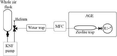
Figure 1 Schematic of the direct trapping system. The flask (NOAA design, 2L, Normag, Germany) is attached (½” ultratorr) to the pump (KNF N86KN.18, KNF Neuberger UK Ltd), the sample is extracted via a phosphorus pentoxide water trap via a mass flow controller (MFC, red-y smart series, GSC-B4SS-BB23, 0–600 mL/min, G1/4”, Icentra, UK) directly to the zeolite trap (13X) of the AGE3 system. The AGE3 is showed simplified here (see (Wacker et al. Reference Wacker, Němec and Bourquin2010c) for full details of this system).
A Luxfer cylinder was filled with dried ambient air for 14C analysis (408.2 ppm), using a SA-6 pump (200 bar, 50 L) at the School of Chemistry, University of Bristol April 29, 2016. This cylinder had a similar CO2 mole fraction to in situ ambient atmospheric samples. This in-house air reference cylinder will henceforth be referred to as the reference tank.
A number of samples (n = 38) from our in-house reference tank were analyzed using this new method. In addition to these 38, seven samples extracted on the system in the initial testing phase were used. These have not been included in the subsequent analysis, all other samples extracted for 15 min at 180 mL·min–1 were included in the analysis. Radiocarbon “dead” CO2 gas (14CO2-free 400 ppm in zero air, purchased from BOC) was used as a processing blank and inter laboratory comparison samples (n = 11) were used as further quality control air standards. Normalization and AMS quality control standards, Oxalic acid II (NIST SRM 4990C) (OXII), IAEA-C7 oxalic acid and phthalic anhydride chemical blank (each at the equivalent of 500 μg C), were prepared by combustion in an elemental analyzer interfaced to the AGE3.
Measurements were performed on a MICADAS AMS system (Synal et al. Reference Synal, Stocker and Suter2007; Wacker et al. Reference Wacker, Bonani, Friedrich and Vockenhuber2010a). Data reduction was performed using BATS software (Wacker et al. Reference Wacker, Christl and Synal2010b). The F14C values generated were converted to Δ14C using Equation 1, correcting for mass dependent fractionation and age (Stuiver and Polach Reference Stuiver and Polach1977) where x is the year of sample collection.
 $$\({\Delta ^{14}}C = ({F^{14}}C{e^{((1950 - x)/8267)}} - 1) \times 1000\)$$
Samples were analyzed until the OXII standards had achieved greater than 500,000 counts of 14C.
RESULTS AND DISCUSSION
Full characterization of the sample pretreatment was carried out. This involved: (1) investigation of the trapping efficiency under different conditions, (2) multiple analyses of air from the in-house reference tank to assess the precision of the method, and (3) comparison to other laboratories to examine the accuracy of the method.
Trapping Time
To determine the optimal length of time required to trap CO2 from a 2 L whole air sample in a glass flask, the trapping time was varied under different conditions. Samples were extracted directly, both from glass flasks filled from the reference tank, and directly from the reference tank itself over a range of flow rates. The zeolite trap temperatures and the measured mass of CO2 trapped were recorded (Figure 2). The AGE3 system is designed to isolate CO2 from combusted samples from the Elemental Analyzer (EA) in a stream of helium carrier gas, at a flow rate of 180 mL/min. The samples extracted from flasks with a maximum flow rate set at 180 mL/min (this flow rate drops as the pressure of the flask is reduced). The samples extracted from the flasks (blue) demonstrated a plateau at 10–20 min, at 400 µg C, indicating complete isolation of the CO2. The flask trapping experiment was continued after the plateau was observed to ensure all of the sample had been trapped. A slight increase was seen from 20 to 25 min, there are two possible reasons for this: either the flasks used in these experiments were filled to slightly higher pressures than those tested at 10–20 min therefore the plateau would have been slightly higher, or at this point, the large pressure difference between the flask (lower than ambient pressure) and the laboratory a leak into the system via the pump or flask attachment may have occurred.
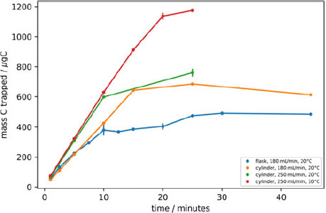
Figure 2 Time varying trapping recording the masses of C trapped on the zeolite, direct from flask at 180 mL·min–1 (blue), direct from cylinder at 180 mL·min–1 (orange), 250 mL·min–1 (green), 10°C (red). The uncertainty of each data point is represented as the standard deviation of repeat measurements (n = 2).
To improve counting statistics and therefore improve the analytical precision, larger samples could be prepared (i.e. 1 mg C instead of 0.5 mg) by filling and sampling 2L flasks in pairs, or filling flasks of larger volumes or at higher pressures. With larger samples however, there is the potential risk of CO2 breakthrough in the zeolite trap due to its saturation. To determine the trapping capacity of the zeolite, samples from the in-house reference tank were extracted directly from the reference tank cylinder at a flow rate of 180 mL/min (orange), ensuring that sample size was not a limiting factor. A linear increase in the quantity of CO2 trapped was observed over the initial 20 min of trapping, however, after this period, at ~685 µg C a plateau was observed due to breakthrough of CO2 since the zeolite trap had reached its capacity under these conditions. The flow rate was increased to 250 mL/min (green), and again, a linear increase was observed initially, until the same plateau level was reached at 760 µg, but after a shorter sampling time. The temperature of the zeolite trap was reduced to 10°C from an ambient trapping temperature (20°C), and the capacity of the zeolite trap was observed to increase to 1200 µg (red).
Sample Uncertainty
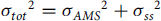
Multiple flasks filled from the reference tank were extracted for 15 min, at 180 mL/min, with the zeolite trap at 20°C. The extraction was performed on 38 samples. The weighted average of Δ14C values was determined as –3.45 ± 0.3‰. For each sample, the uncertainty of the measurement was plotted as the uncertainty (σtot) for individual measurements (Figure 3). The uncertainty includes instrument error (σAMS) that incorporates counting statistics, normalization errors and blank uncertainties. Generally, a sample scatter factor (σss) (Equation 2), will be added using a sum-of-squares approach. This sample scatter factor is determined using chi-squared tests on repeat measurements. This accounts for any additional uncertainty resulting from sample preparation including graphitization and extraction (observed as scatter in the repeat analysis of a standard).
 $$\(\vskip 10pt{\sigma _{tot}}^2 = {\sigma _{AMS}}^2 + {\sigma _{ss}}^2\)$$
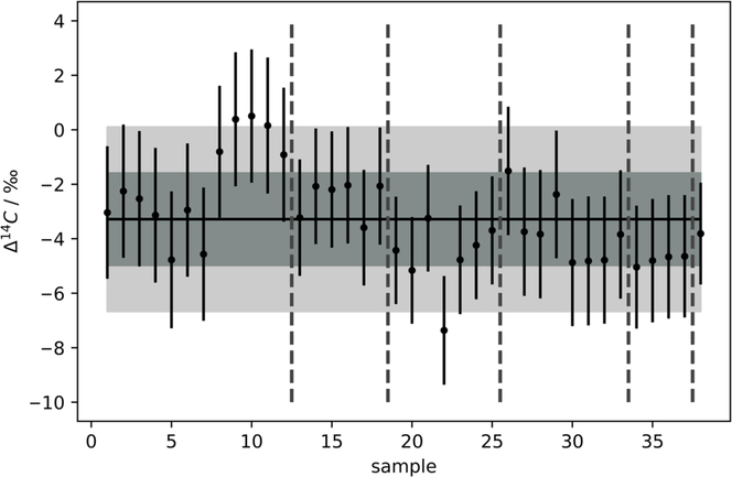
Figure 3 Δ14C values determined for the in-house reference standard extracted for 15 min at a max. flow rate of 180 mL·min–1 for 38 samples, 1σ (grey, 1.97‰) and 2σ (pale grey, 3.94‰). Mean represented by solid black line (Δ14C = –3.45‰). All measurements were within 2σ. Vertical grey dashed lines separate measurements from different AMS magazines.
Assessment of Sample Uncertainty Contributions
The 38 samples extracted using our new direct zeolite trapping method were measured across 6 magazines from October 2017 to August 2018 (Table 1). We performed a Pearson’s chi-squared test to assess how well the observed distribution of data fits with the distribution that would be expected if the variables are independent. The right-tailed p-value (α) calculated for this distribution was 0.87, suggesting that the instrument uncertainty accounts for all observed scatter. If a sample scatter value was to be added, the errors would be overestimated. It is likely that the uncertainty is currently dominated by the scatter in Oxalic Acid II standards that are prepared by combustion in the EA. The blanks from the EA method were also used in the calculation of the sample uncertainty. This is because the standard deviation of the oxalic acid was 2.5‰, larger than that of the reference samples which was 1.7‰. It is likely that the EA combustion step introduced a larger degree of sample scatter to these standards than was observed in air samples. In the future, we will investigate this further by using air standards containing CO2 from bomb-combusted oxalic acids and blanks to determine a truer precision of the method.
Table 1 Details regarding the AMS magazines containing samples measured as part of this study.
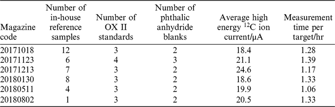
The instrument uncertainty (σAMS) for each sample was therefore, used as the total analytical uncertainty for this study. The average uncertainty across the 38 replicate analyses was 2.0‰ (on the Δ14C scale).
Blank Analysis
Extraction of air “blanks,” consisting of zero-air mixed with radiocarbon dead CO2, using the direct zeolite trapping method produced an average value of 0.76 ± 0.13 pMC, calculated based on measurements of blank samples independent from contamination from ambient samples (n = 15). The purpose of these blank analyses was to enable identical sample pretreatment of all standards. The data for these were higher than the Phthalic Anhydride blank prepared using the EA (0.34 ± 0.07 pMC). This is lower than observed from the isolation of our radiocarbon “dead” air standard, suggesting some contamination; the source of this is yet to be confirmed. All samples in this study contained ca. 400 μg C, resulting in a slightly higher blank than would be observed for typical full-sized samples (1 mg C).
Cross Contamination
“Modern” in-house reference samples were extracted and graphitized immediately preceding radiocarbon “dead” samples to examine the effect of cross contamination between samples. Four sequences consisting of three blanks following a sample from the in-house reference tank (Δ14C = –3.45‰) were extracted, and the data are presented in Figure 4. The first blank of each sequence was observed to be higher than the second and third.
Figure 4 Cross-contamination tests. Four sets of three consecutive radiocarbon blanks isolated and graphitized after a sample of our (modern) in-house reference gas. A cross-contamination level of 1.83 ± 1.52‰ was calculated using a simple mixing model. The mean value for the first blank after the reference was 0.942 ± 0.077 pMC, second blank was 0.803 ± 0.129 pMC and third blank was 0.721 ± 0.102 pMC.
Cross contamination can be described by a simple mixing model. A measured pMC value of the blank sample (X, 0.942) depends linearly on the previous measured sample (s0, 100.45) and the “true” pMC value of the blank (s1, 0.76), the cross-contamination level (c), is the coefficient for the previous sample.
 $$\(c = {{X - s_1} \over {s_0 - s_1}}\)$$
A cross-contamination level of 1.83 ± 1.52‰ (or 0.183 ± 0.152%) was determined using Equation 3, which is significantly higher than that reported by Wacker et al. (Reference Wacker, Němec and Bourquin2010c) (0.6 ± 0.1‰). Therefore, as with the EA-AGE3 system, when analysing samples with very different levels of 14C, the zeolite should be pre-conditioned with a sample of similar 14C content. The ‰ cross contamination is in parts per thousand. Therefore, 0.183% of the C in one sample comes from the sample before. For example, if two samples have a difference in Δ14C of 10‰, the second sample will be shifted by 0.0183‰ on the Δ14C scale. To establish the amount of C from the sample transferred to the 2nd blank processed subsequently, the “effective c” value of this blank was calculated to be 0.43‰. The “real c,” calculated from the first blank cannot be changed regardless of the approach taken, whereas the effective c can change depending on the approach used (e.g. 1st + 2nd blank). This agrees with the findings of Wacker et al. (Reference Wacker, Němec and Bourquin2010c) and demonstrates the efficacy of a sacrificial sample (of similar 14C content to subsequent samples) between samples of very different 14C content when using this system.
Inter-Laboratory Comparisons
Of great importance to atmospheric 14C laboratories, and 14C laboratories in general is inter laboratory comparisons to confirm that laboratories are reporting with the same accuracy and give realistic values for precision. These exercises, though of great importance for global monitoring, rarely happen (Miller et al. Reference Miller, Lehman, Wolak and Kondo2013; Hammer et al. Reference Hammer, Friedrich, Kromer and Uchida2017).
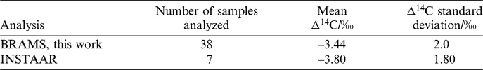
The results of our determination on the in-house reference standard were compared to seven flasks of the same reference tank analyzed at an independent AMS laboratory, the Institute of Artic and Alpine Research (INSTAAR), which has a long history of making atmospheric 14CO2 measurements. These data are shown in Table 2. The average Δ14C values are comparable within 1σ.
Table 2 Summary of our in-house reference standard extracted and measured at two different laboratories, Bristol Radiocarbon Acceletor Mass Spectrometer facility (BRAMS) and Institute of Artic and Alpine Research (INSTAAR).
Samples (n = 4) that previously were analyzed at the Integrated Carbon Observation System Central Radiocarbon Laboratory (ICOS-CAL), in Heidelberg, Germany were also analyzed on our new direct trapping extraction system. These samples were part of a previous inter laboratory comparison study (Hammer et al. Reference Hammer, Friedrich, Kromer and Uchida2017), therefore have been measured at multiple laboratories. The results of the analyses from this study were compared to the consensus values from the inter-comparison study, presented in Table 3. Samples were split into two aliquots to enable replicate measurements. Unfortunately, for samples 30864 and 30874 analysis of only one aliquot was possible. For samples 30996 and 31061 both aliquots were analyzed. The results presented in Table 3 are a weighted mean of these. Although all measurements were within 2 σ (and three of the four samples were within 1σ), all of the measurements from this study were found to be slightly lower than the consensus value. The limited size of the dataset makes interpretation of this difficult, however if there is a systematic offset it could point to a small amount of contamination with atmospheric CO2 during a leak to the system or may be because of the lower blank values. Further analysis will be required to establish this. The uncertainties reported for the consensus values are lower than any of the measurements by individual labs (including those reported here) as they were calculated based on multiple measurements at several laboratories. The uncertainties reported in this paper are similar in magnitude to the standard deviation of the measurements of the inter-comparison study at the individual laboratories, meaning this is dependent on the factors outlined above due to the combustion of the Oxalic Acid standard.
Table 3 Four of the samples used in the inter comparison (Hammer et al. Reference Hammer, Friedrich, Kromer and Uchida2017) measured during this study and the intercomparison consensus values. The chi-squared right-tailed P value for each sample is also reported.
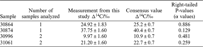
The right tailed chi-squared p values for each measurement shows that there is no significant difference in the measurements in this study and the consensus values. A significance level of 5% was used (p = 0.05) and all p values were higher than this, meaning the null hypothesis was true and there is agreement between the measurements in this study and the consensus values within errors. This analysis was performed on a small number of samples and further comparisons with be required to ensure measurements between laboratories are comparable. The World Metrological Organisation (WMO) Guidelines state that current compatibility between laboratories is 2–4‰, short of the goal of 0.5‰ (Tans and Zellweger Reference Tans and Zellweger2016). The comparisons made in this paper are comfortably within the compatibility reported in the WMO guidelines (2–4‰) as are comparable to a level of 2.7‰, which is the largest difference in the inter comparison experiments. Overall, our new set up has shown comparable compatibility to other AMS laboratories making atmospheric 14CO2 measurements from other studies (Hammer et al. Reference Hammer, Friedrich, Kromer and Uchida2017).
CONCLUSION
We have developed and reported an alternative method for the extraction of atmospheric 14CO2 samples. It is anticipated that this method, with the graphitization and analysis for 14C using AMS, will be used for the analysis of multiple samples for quantifying fossil fuels CO2 emissions in the UK. Our initial results are promising for the future of these measurements, demonstrating agreement with other 14C laboratories. We have reported a range of tests that have characterized the direct trapping system. A trapping capacity of 400 µg C in 15 min at 180 mL·min–1 from a 2 L flask has been achieved. The trapping capacity at room temperature achieved was 685 µg. The trapping capacity at 10°C was 1200 µg. In this work, the maximum flow rate investigated for trapping on the zeolite trap was 250 mL / min. This method has been used for pretreatment of 38 replicate samples to achieve standard deviation on long term measurements of 2.0‰ over 6 magazines. Assessment of the uncertainty suggests the use of an air sample containing OXII-derived CO2 rather than OXII prepared by EA-AGE3 could be advantageous as a normalization standard. Blank analysis shows that the cross-contamination level is 1.83 ± 1.52‰, meaning if analyzing samples with very different levels of 14C, the zeolite should be pre-conditioned with a sample of similar 14C content. Analysis of inter-comparison samples showed this method is comparable to two other global radiocarbon laboratories to a level of 2.7‰, within the WMO guidelines (2–4‰). In the future, we will fully characterize the system to further investigate why the air blank is higher than the combustion blank, and why the memory effect of our line and its uncertainty are much higher than those reported in Wacker et al. (Reference Wacker, Němec and Bourquin2010c). We then aim to automate the whole extraction process, integrating this to the AGE3 system to increase sample throughput and precision, vital for atmospheric 14CO2 measurements.
ACKNOWLEDGMENTS
The authors would like to acknowledge Samuel Hammer for providing samples of his inter-comparison study to test our system. This work was supported by the Natural Environment Research Council [NE/L002434/1]. We thank the two reviewers and the Radiocarbon editors for their helpful advice in improving this manuscript.


