


1. Introduction
Large numbers of positrons have the potential to enable a wide variety of new experiments (Hugenschmidt Reference Hugenschmidt2016), including the ‘A Positron Electron eXperiment’ (APEX) collaboration's goal to create and study strongly magnetized low-energy positron–electron plasmas (Stoneking et al. Reference Stoneking, Pedersen, Helander, Chen, Hergenhahn, Stenson, Fiksel, von der Linden, Saitoh and Surko2020). These so-called pair plasmas are predicted to be remarkably stable in the targeted magnetic confinement geometries (Helander Reference Helander2014), and phenomena commonly occurring in electron–ion plasmas due to their mass asymmetry are predicted to be absent (Stenson et al. Reference Stenson, Horn-Stanja, Stoneking and Pedersen2017). This makes such plasmas an extraordinary candidate to test basic theories of plasma physics.
The bottleneck in the pair-plasma creation is the accumulation of sufficient numbers of low-energy positrons. Usually, large numbers of positrons are accumulated and confined using a Penning–Malmberg (PM) configuration. These configurations are made of cylindrical electrodes in a strong magnetic field where this field is used for the radial, and electric potentials for the axial confinement (Malmberg & deGrassie Reference Malmberg and deGrassie1975). The current record, achieved in a single PM trap, lies at $4\times 10^9\,$ e$^+$
e$^+$ (Jørgensen et al. Reference Jørgensen, Amoretti, Bonomi, Bowe, Canali, Carraro, Cesar, Charlton, Doser and Fontana2005; Fitzakerley et al. Reference Fitzakerley, George, Hessels, Skinner, Storry, Weel, Gabrielse, Hamley, Jones and Marable2016; Niang et al. Reference Niang, Charlton, Choi, Chung, Cladé, Comini, Crivelli, Crépin, Dalkarov and Baker2020).
Scaling this up further in the same type of PM trap is inherently challenging, because the plasma space-charge potential $\phi _P$ on-axis is proportional to the charge per unit length,

where $N$ denotes the number of particles (i.e. positrons), $e$
 the elementary charge, $\epsilon _{0}$
 the vacuum permittivity, $l_P$
 the plasma length, $r_P$
 the plasma radius and $r_W$
 the inner wall radius of the trap. To ensure confinement, the confinement potential $\phi _C$
 must be larger than the plasma potential; i.e. $|\phi_{P}\,(r=0)| < |\phi_{C}\,(r=0)|$
 . Hence, the accumulation of 10 times as many particles requires 10 times higher potentials or 10 times longer plasmas, both of which present severe experimental challenges (Danielson & Surko Reference Danielson and Surko2006; Danielson et al. Reference Danielson, Dubin, Greaves and Surko2015). Since APEX needs $10^{10}$
 to $10^{11}$
 low-energy positrons to access a regime where collective effects are observable (Stoneking et al. Reference Stoneking, Pedersen, Helander, Chen, Hergenhahn, Stenson, Fiksel, von der Linden, Saitoh and Surko2020), this would mean $\phi _C\sim {\rm kV}$
 or $l_P\sim {\rm m}$
 in a conventional PM trap.
An attractive alternative is to separate the plasma space charge into a multi-cell trap (MCT) configuration (Surko & Greaves Reference Surko and Greaves2003). Consisting of one large-diameter PM trap (the ‘master cell’) and multiple smaller on- and off-axis PM traps (the ‘storage cells’), plasmas initially captured in the master cell are subsequently transferred to the storage cells. The problems that arise with high space charges or long plasmas are mitigated by separating the number of positrons into different volumes. These storage cells can be fit into the same magnetic field volume by using a hexagonal-close-packed arrangement. By contrast, making a large-diameter single cell would not have the same benefit, due to the logarithmic dependence in (1.1).
The first prototype MCT was developed and built at University of California, San Diego, and several of the necessary techniques for its operation were established. The plasma displacement using the autoresonant excitation of the diocotron mode (Baker et al. Reference Baker, Danielson, Hurst and Surko2015; Hurst et al. Reference Hurst, Danielson, Baker and Surko2015) was used to precisely address the off-axis cells. The plasma dynamics of the transfer process was determined (Hurst et al. Reference Hurst, Danielson, Baker and Surko2014), and the functionality of the MCT concept was demonstrated by transferring and confining plasmas in each of several storage cells (Hurst et al. Reference Hurst, Danielson, Baker and Surko2019).
However, a couple of essential points remained to be addressed: a suitable protocol is needed for the consecutive transfer of plasmas, with minimal particle losses, to multiple off-axis storage cells. Good confinement in the off-axis storage cells must be demonstrated, as a prerequisite for the stacking of multiple pulses in each off-axis cell and, ultimately, the creation of a plasma with larger $N$ and $\phi _{P}$
 . While the MCT concept aims to avoid $\phi_C \sim\,$
 kV, Apex will require $N \sim 3\times 10^{9}\,{\rm e}^{+}$
 per cell and $|\phi_{C}| \ge |\phi_{P} \,(r_{P}=1\,{\rm mm}, \ l_{P} = 100\,{\rm mm}, \ N=3\times 10^{9}\,{\rm e}^{+})| \sim 200\,{\rm V}$
 . Finally, ejection of the off-axis plasmas and transfer to the pair-plasma experiments (or other experiments with a need for large positron pulses) must be worked out. A second prototype MCT has been constructed at the Max-Planck-Institute for Plasma Physics to address these challenges.
The present article describes the achievement of recent milestones in the MCT development. Section 2 introduces the second prototype MCT and its diagnostics, and § 3 describes calibration and commissioning. Adaption of the master-cell alignment routine (Singer et al. Reference Singer, König, Stoneking, Steinbrunner, Danielson, Schweikhard and Pedersen2021) to the new geometry is addressed in § 4. Section 5 describes electron plasma creation with a LaB$_6$ emitter, followed by a discussion of confinement limits in § 6. Findings involving competing diocotron drifts in the new trap arrangement are shown in § 7, and the on- and off-axis transfer from the master cell into the storage cells is discussed in § 8. Furthermore, we present the plasma confinement in the storage cells in § 9, then, in § 10, we summarize our findings and discuss remaining steps toward a high-capacity MCT.
2. The second prototype MCT
Following successful experiments with a master-cell test trap (Singer et al. Reference Singer, König, Stoneking, Steinbrunner, Danielson, Schweikhard and Pedersen2021), that apparatus has been rebuilt and extended to become the new prototype MCT. This second prototype MCT is installed in vacuum (${\sim }2\times 10^{-9}$ to $4\times 10^{-9}$
 mbar) in the room-temperature bore of a superconducting magnet (Oxford, presently up to 3.1 T on axis). The trap sits on support bars which are fastened in the flange on one side to fix its position within the apparatus.
Figure 1 shows a schematic of the MCT overlaid with the on-axis magnetic field (blue dots), where $z=0$ mm denotes the centre of the homogeneous field region. Three storage cells are currently installed: the on-axis cell (${\rm S}_{2}$
 ) and two which are displaced $25.9$
 mm off axis (${\rm S}_{1}$
 and ${\rm S}_{3}$
 ). Each has an inner wall radius of $r_{W,S}=6$
 mm, a total length of $L_{S}=130$
 mm and consists of five electrodes (e.g. ${\rm S}_{1.1}$
 to ${\rm S}_{1.5}$
 ). In each cell one electrode is azimuthally segmented and used for plasma diagnostics and manipulations; ${\rm S}_{1.2}$
 has four segments, as does ${\rm S}_{2.4}$
 (which is positioned at a different axial location to prevent cross-talk at the contacts), while ${\rm S}_{3.2}$
 has eight (for comparison studies). The master cell (electrodes M1 to M6) has an inner radius of $r_{W,M}=37$
 mm and total length of $L_{M}=281$
 mm; M2 is fourfold segmented. Between the storage cells and the master cell is the independently controlled transition electrode TE, which has apertures that line up with the inner diameters of the storage cells. The apertures are arranged in a hexagonal closed-pack geometry (Surko & Greaves Reference Surko and Greaves2003), anticipating future expansion to a total of seven storage cells. The trap is located within the homogeneous field region, except for M6, which is usually connected to ground to prevent the potential applied to the phosphor screen from affecting the plasma trapped in the master cell.

Figure 1. Schematic drawing of the MCT, overlaid with a plot of the axial magnetic field strength (blue dots). From left to right are the emitter (in the fringe field of ${\sim }2.55$ T), the three storage cells (${\rm S}_{1}$
 , ${\rm S}_{2}$
 and ${\rm S}_{3}$
 ), the transition electrode (TE), the master cell (electrodes M1 to M6) and the phosphor screen (also in ${\sim }2.55$
 T).
T).
All electrodes are made of aluminium, and surfaces visible to the plasma are coated with colloidal graphite, so as to avoid patch potentials that would cause radial transport (Robertson, Sternovsky & Walch Reference Robertson, Sternovsky and Walch2004; Natisin, Danielson & Surko Reference Natisin, Danielson and Surko2016). Each electrode stack is clamped between mounts at each end, pulled together with rods. Each storage-cell stack has four set screws, used to apply individual clamping forces, to make it possible to align all the cells at once. This addresses a key issue raised by the first prototype MCT, in which simultaneous alignment of multiple storage cells proved difficult to achieve (Hurst et al. Reference Hurst, Danielson, Baker and Surko2019).
A phosphor screen is installed in the fringe field at one end of the trap, an electron emitter at the other, both at magnetic fields of approximately 2.55 T. The experiments described here were performed with electrons from a lanthanum hexaboride (LaB$_6$ ) crystal emitter (Applied Physics Technologies). This emitter has a flat-top design with a circular emission surface 1 mm in diameter that is conductively heated through two graphite blocks; it produces high emission currents at low heating currents and voltages, due to its lower work function (Wenzel et al. Reference Wenzel, Schlisio, Mulsow, Pedersen, Singer, Marquardt, Pilopp and Rüter2019), thereby producing less background light which can influence phosphor screen measurements. The phosphor screen (Dr. Gassler Electon Devices) is the primary diagnostic, used to measure the electron number $N$
 and the $z$
 -integrated plasma density. It is made of P43 phosphor (Gd$_{2}$
 O$_{2}$
 S:Tb) deposited on an $x$
 -ray safety glass coated with a transparent conducting layer of indium tin oxide (ITO). The emission peak of this phosphor is at 545 nm (green), which matches the maximum quantum efficiency (${\sim }70\,\%$
 at 545 nm) of the CMOS camera (Cygnet Cy4MP-CL) used to image it.
The experimental cycles are controlled with a pulsed-pattern generator, based on a field-programmable gate array (FPGA) (Ziegler et al. Reference Ziegler, Beck, Brand, Hahn, Marx and Schweikhard2012; Singer et al. Reference Singer, König, Stoneking, Steinbrunner, Danielson, Schweikhard and Pedersen2021). They comprise fill, hold and manipulate and dump periods. A typical cycle starts with the plasma creation in the master cell, followed by feedback damping of the residual diocotron mode (Malmberg et al. Reference Malmberg, Driscoll, Beck, Eggleston, Fajans, Fine, Huang and Hyatt1988) to centre the plasma in the master cell. Then the plasma is manipulated by, e.g., autoresonant excitation of the $m=1$ diocotron mode (Fajans, Gilson & Friedland Reference Fajans, Gilson and Friedland1999) and/or transfer to the off-axis cells. (Compression of the plasma using rotating electric fields (Danielson & Surko Reference Danielson and Surko2006) is also possible, but it was not employed for the present experiments.) In the final step, all electrodes between the plasma and the screen are rapidly (${\le }1\,\mathrm {\mu }$
 s) grounded so that the plasma is accelerated onto the phosphor screen to be destructively diagnosed.
3. Phosphor screen calibration
When measuring the two-dimensional (2-D) plasma distribution, the screen is biased to $+$ 5 kV. A super-Gaussian fit is applied to the measured signal to determine the central density $n_0$
 , plasma radius $r_P$
 and its position $(x,y)$
 (Singer et al. Reference Singer, König, Stoneking, Steinbrunner, Danielson, Schweikhard and Pedersen2021). The latter two need the factor $\kappa$
 for the conversion from pixel to mm. It is obtained by autoresonantly exciting the $m=1$
 diocotron mode in the master cell, using a rotating, sinusoidal, frequency-chirped dipole field (Singer et al. Reference Singer, König, Stoneking, Steinbrunner, Danielson, Schweikhard and Pedersen2021). Due to the changing position of the screen during the alignment (topic of the next section), the calibration is usually performed afterwards.
The diocotron excitation is applied until the plasma is in contact with the master-cell electrodes, followed by an ejection onto the screen. By repeating this procedure for different phases a projection of the master cell's inner wall is obtained. This provides a direct projection of the trap's boundary within the homogeneous magnetic field onto the screen in the fringe field, thereby including the expansion of the magnetic flux. A circular fit is applied to the outer plasma edges and the diameter of this circle in relation to twice the wall radius $r_{W,M}$ gives us the conversion factor $\kappa = 74.2(5)\,\mathrm {\mu }$
 m pxl$^{-1}$
 . The same method is used in ${\rm S}_{2}$
 to determine its position.
Figure 2 shows the camera view through the vacuum window onto the phosphor screen. The background image shows its field of view after the alignment. Each circle or elliptical spot represents a separate measurement. The colour indicates the plasma density. The dark blue plasmas at the larger radii are from measurements to determine $\kappa$ . These plasmas are displaced far off axis, quite expanded and are losing particles by touching the electrodes. The black dashed line is the circular fit to the data with the small black dot marking the middle of the circle. The bright yellow–green spots represent plasmas used to obtain the position of the storage cells (as explained below) and the red dashed lines represent fits to determine the storage cells inner wall.
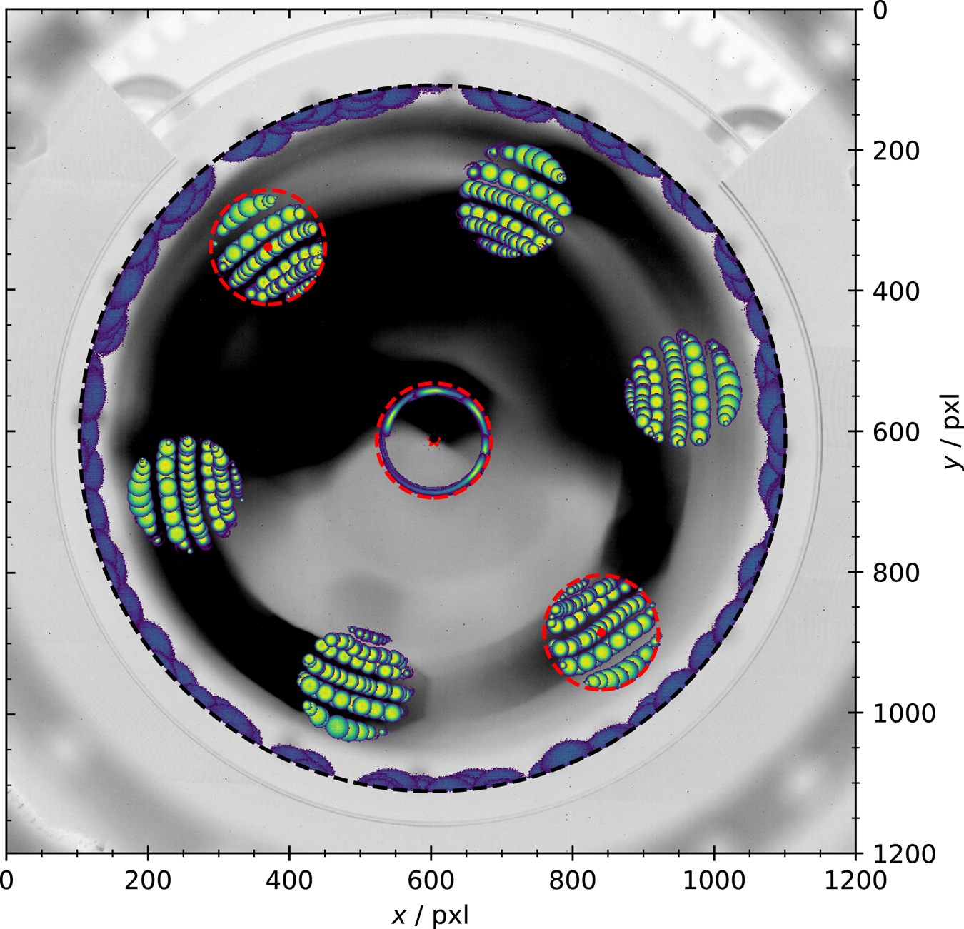
Figure 2. Full camera view of the phosphor screen. In blue are repeated measurements of plasmas which are displaced up to the master-cell wall for different phases. This is repeated in the middle for the on-axis storage cell. The black dashed line shows a fit to the outer edges of those plasmas to determine the master-cell wall position as well as the pixel to mm conversion factor $\kappa = 74.2(5)\,\mathrm {\mu }$ m pxl$^{-1}$
 . In green, plasmas are shown which are displaced off-axis to determine the off-axis cell positions. The red dashed lines are the derived positions of the off-axis storage cells with the red dots or star marking their respective centres.
In the centre of figure 2 this measurement is repeated in the on-axis storage cell ${\rm S}_{2}$ , to picture the edges of its wall. A circular fit is applied (red dashed line) to determine its position. The centre of ${\rm S}_{2}$
 (red cross) is slightly displaced from the centre of the master cell. This is consistent with the alignment measurements (next section) and can be related to the tolerance (${\pm }0.05$
 mm) given when the trap was fabricated. The deformation of the plasmas in ${\rm S}_{2}$
 is due to a linear voltage ramp to the designated amplitude at the beginning of the excitation. This was done to prevent ‘kicking’ the plasma out of the centre, reducing the reproducibility of the excitation. In the master cell the ramp's influence on the plasma is small due to the large $r_{W,M}$
 . In ${\rm S}_{2}$
 the electrodes are closer to the plasmas, so that the ramp results in a distortion of the plasmas shape due to the applied potentials (Chu et al. Reference Chu, Wurtele, Notte, Peurrung and Fajans1993).
Since the design of the trap allows for rotation around the axis of symmetry of the master cell during the assembly, determining the exact position is necessary for transfer experiments. The technique developed to measure the exact position has four steps: first, a plasma is created in the master cell and the residual diocotron motion is feedback damped. Second, the diocotron mode is autoresonantly excited for a defined time, displacing the plasma radially. Third, the confinement potential at M1 and TE is rapidly grounded for $20\,\mathrm {\mu }$ s, letting the plasmas expand into the direction of the storage cells. Now the plasma either comes in contact to the grounded electrode TE (black parts of TE in figure 1) and gets destroyed, or it expands into one of TE's apertures and survives. Fourth, the confinement field at M5 is rapidly changed, accelerating the plasma onto the screen, resulting in a picture of the plasma if it survived the third step. These four steps are repeated for increasing excitation times i.e. different displacements.
This technique results in a projection of the transversal storage-cell position on the phosphor screen. The result of such measurements is shown in figure 2. Each yellow–green plasma profile presents one measurement cycle described above, where the plasma expands into the storage cell region and survives. While there are only two off-axis cells currently installed, the technique pictures all six off-axis apertures in TE. These measurements are now used to determine the position and centre of ${\rm S}_{1}$ and ${\rm S}_{3}$
 by applying a circular fit to respective regions (red dashed lines). This provides the position of the off-axis cells to an accuracy of $({\rm \Delta} x,{\rm \Delta} y)=(37,74)\,\mathrm {\mu }$
 m. Judging from figure 2, this technique can easily be extended to picture more storage cells, even on different radial displacements; which is necessary for some designs recently proposed (Witteman et al. Reference Witteman, Singer, Danielson and Surko2023).
The screen is not only used to picture the 2-D plasma distribution, but also as a charge collector to measure the number $N$ of electrons of the confined plasma. When used as a charge collector, either the total charge is measured using a commercial charge integrator (CREMAT CR-113), with the screen at 500 V. Or the dump pulses are decoupled from the high DC voltage using a custom-built RC-circuit, providing a non-calibrated relative charge measurement for the $N$
 . Both techniques give similar results as confirmed by many comparative measurements. The RC-circuit was built so that it can be biased up to 5 kV. Meaning, that it can give a reliable measurement of the relative $N$
 simultaneous with the measured 2-D plasma distribution.
4. Magnetic field alignment
To align the trap to the magnetic field, as it is necessary to achieve long time confinement (Witteman et al. Reference Witteman, Singer, Danielson and Surko2023), a technique is adapted (Aoki et al. Reference Aoki, Kiwamoto, Soga and Sanpei2004; Singer et al. Reference Singer, König, Stoneking, Steinbrunner, Danielson, Schweikhard and Pedersen2021) that uses the residual $m=1$ diocotron mode, which is a remnant from the filling procedure. Repeated measurements of the mode's amplitude at different $z$
 -positions provide a fast and direct measure of the misalignment and its direction. This is a great advantage compared with using time intensive confinement measurements. Since the best confinement is desired in the storage cells, the adaptation of this technique to the alignment of the MCT will focus on the on-axis cell. The idea is to align the on-axis cell and, since all three cells are built to be parallel, simultaneously aligning the off-axis traps.
The measurements are performed at three different positions: ${\rm S}_{2.2}$ , ${\rm S}_{2.5}$
 and M5. These are the positions of the grounded electrodes where plasmas are confined. The electrodes of ${\rm S}_{2.2}$
 and ${\rm S}_{2.5}$
 are the primary positions for the alignment. They have the same length and inner wall radius and are axially separated approximately ${\rm \Delta} z_1=69$
 mm from one another. Measuring in M5, at a distance of ${\rm \Delta} z_2=285$
 mm from ${\rm S}_{2.2}$
 , indicates whether the master cell's end facing the screen is parallel to the storage cells. The residual diocotron mode is measured in those volumes, the position and amplitude are compared, and then the vacuum chamber's position is adjusted accordingly, and the measurements are repeated. The aim is to adjust the alignment until the centres and amplitudes match.
The outcome of this procedure is shown in figure 3. It contains measurements of the residual diocotron mode in ${\rm S}_{2.2}$ (blue), ${\rm S}_{2.5}$
 (orange) and M5 (black) after the alignment. In the $xy$
 -plane the individual position measurements (points) and circular fits to the data (lines) are visualized. The blue dot, and orange and black crosses in the middle mark the corresponding centre position to the fits. Assuming that the inner walls of the confining electrodes are parallel to each other and the magnetic field lines are straight, the distance between the centres ${\rm \Delta} C$
 corresponds to an angular misalignment ${\rm \Delta} \zeta$
 via ${\rm \Delta} \zeta = \arctan ({{\rm \Delta} C}/{{\rm \Delta} z})$
 . Using the alignment routine, the distance between the centres of ${\rm S}_{2.2}$
 and ${\rm S}_{2.5}$
 is reduced to ${\rm \Delta} C_1 = 1(14)\,\mathrm {\mu }$
 m which corresponds to a misalignment of ${\rm \Delta} \zeta _1 = 1(3)$
 mdeg. This is within the measurement's uncertainty. At this optimized position the centre distance between ${\rm S}_{2.2}$
 and M5 is ${\rm \Delta} C_2 = 15(11)\,\mathrm {\mu }$
 m which yields a misalignment of the whole structure of ${\rm \Delta} \zeta _2 = 3(5)$
 mdeg.
mdeg.
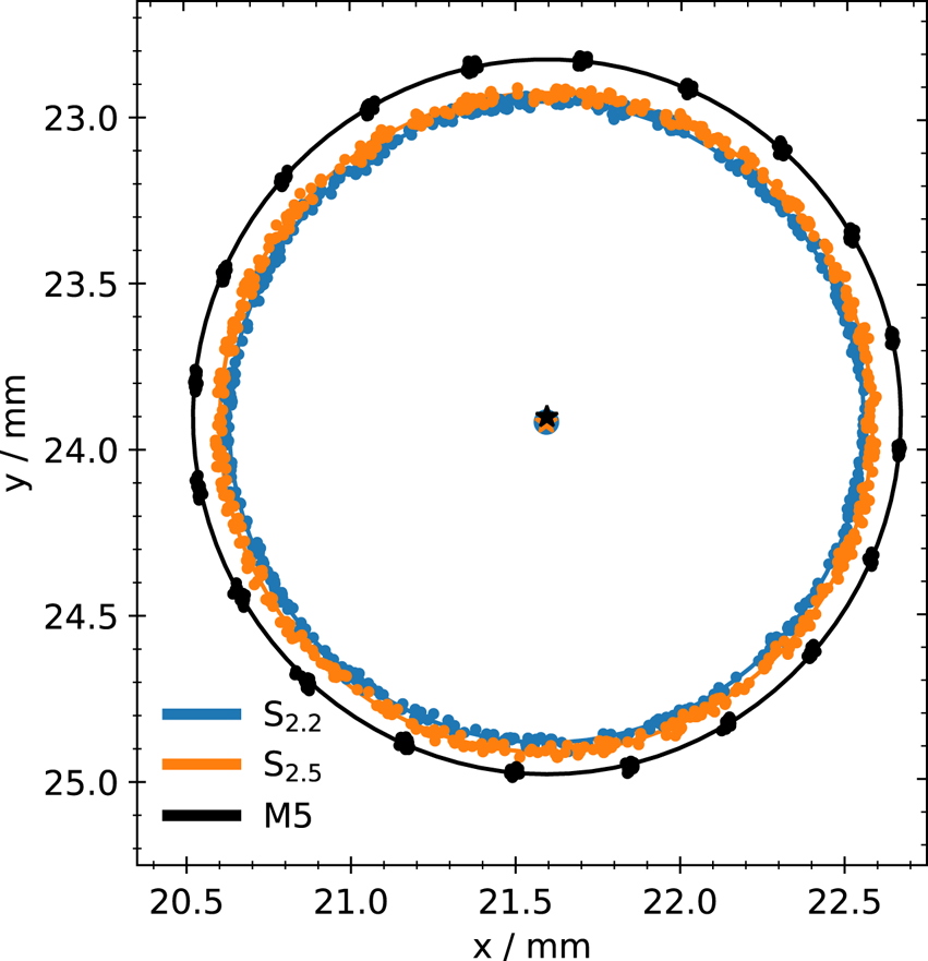
Figure 3. Residual diocotron motion measured in ${\rm S}_{2.2}$ (blue), ${\rm S}_{2.5}$
 (orange) and M5 (black) and their respective circular fits (lines) to determine the centre distances ${\rm \Delta} C$
 . Plotted are the individual position measurements (dots) in the $xy$
 -plane on the screen, as well as the circular fits (lines) and their respective centres (stars and dot).
Since the grounded electrodes of ${\rm S}_{2.2}$ and ${\rm S}_{2.5}$
 have the same wall radius and length they also have the same plasma length and similar densities. The grounded electrode of M5 is longer and has a different wall radius which changes the plasma length and charge per unit length. Since the diocotron motion depends on both of these factors (Fajans et al. Reference Fajans, Gilson and Friedland1999), the amplitude is expected to be somewhat different from the other two as well. Also, as previously mentioned, there is an uncertainty with respect to the fabrication of the trap. This is true for the transition electrode TE from the storage-cell stack to the master cell as well, which could result in a tilt of the master cell compared with the storage-cell stack. These factors influence the comparability of this technique from ${\rm S}_{2.2}$
 and ${\rm S}_{2.5}$
 to M5 and reduce the significance of ${\rm \Delta} \zeta _2$
 . However, if the walls of all three electrodes are parallel to each other, the comparison of ${\rm S}_{2.2}$
 to M5 should still give a good proxy for the alignment of the whole structure.
5. Plasma creation and preparation
For the set of experiments described here, the previous rhenium emitter was exchanged for a lanthanum hexaboride (LaB$_6$ ) crystal emitter. Thus the initial plasmas used here differ from those described previously (Singer et al. Reference Singer, König, Stoneking, Steinbrunner, Danielson, Schweikhard and Pedersen2021). The LaB$_6$
 emitters have a low work function (Wenzel et al. Reference Wenzel, Schlisio, Mulsow, Pedersen, Singer, Marquardt, Pilopp and Rüter2019) delivering high electron currents at low heating currents. Hence, they emit less light which contaminates the phosphor screen measurements, while providing electron currents comparable to the rhenium filament. Using a heating current of $I_f=1.055$
 A at $U_f\approx 2$
 V provides an emission current in the range of $10^{-4}$
 to $10^{-3}$
 A. With these settings high-$N$
 plasmas are created while operating in the regime of fast and reproducible plasma creation and avoiding significant photon pollution of the CMOS camera. For higher heating currents the light emission from the emitter becomes noticeable in the measurements of the 2-D plasma profiles.
To characterize the plasmas created using the new emitter plasma formation measurements in the master cell are performed: the number of electrons $N$ and the 2-D distribution of the created plasma is obtained as a function of the fill time $t_{f}$
 . At the beginning of the measurement all electrodes between the emitter and M5 are grounded. Only M5 is set to $\phi _C=-300$
 V. Electrons streaming from the emitter into the confinement region get reflected at M5 and stream back to the emitter, building up a space-charge cloud between the emitter and M5 (Gorgadze Reference Gorgadze2003; Bettega et al. Reference Bettega, Cavaliere, Cavenago, Illiberi, Pozzoli and Romé2007). After $t_f$
 the potential at M1 and TE is quickly (${\le }1\,\mathrm {\mu }$
 s) switched to $\phi _C$
 , trapping a part of the electron cloud between M1 and M5. The electrons are confined for $300\,\mathrm {\mu }$
 s before M5 is grounded, releasing the trapped electrons onto the phosphor screen. The measurement was repeated for three different emitter bias voltages $U_{B}$
 : $-$
: $-$ 25, $-$
 40 and $-$
 50 V. This voltage cannot be chosen arbitrarily small since the emitter is positioned in the fringe field and the particles need sufficient energy to prevent them from being magnetically mirrored when entering the high-field region (Allen Reference Allen1962). By increasing the bias potential, the acceleration parallel to the magnetic field direction is increased and the pitch angle (angle between the magnetic field and velocity vector) reduced. This reduces the amount of electrons which are mirrored and more particles reach the high-field region. To change the number of trapped electrons, the emitter bias is adjusted instead of the heating current or fill time. When changing the heating of the crystal with $I_{f}$
 it takes a while to reach a new stable equilibrium state. And adjusting $N$
 by choosing a shorter fill time usually leads to a decreased reproducibility. The bias voltage can be adjusted quickly and reproducibly and with it $N$
 .
.
Figure 4 shows the results from the plasma creation measurements versus the fill time $t_f$ , for all three bias voltages. The development of the electron numbers [figure 4(a)] suggest that two-stream interactions occur nearly instantaneously ($t_f<10^{-5}$
 s) due to the high-emission current, quickly filling up the velocity phase space (Gorgadze Reference Gorgadze2003). After $t_f\approx 10^{-4}$
 s a stable space-charge cloud has been created which matches the emitter bias. Due to this fact, the amount of charge can be chosen by adjusting the bias, varying the number of electrons from ${\approx }2.8\times 10^8$
 ($U_B=-25\,$
 V) to ${\approx }6.4\times 10^8$
 ($U_B=-50$
 V). Figure 4(b) shows the corresponding shot-to-shot variability ${\rm \Delta} N/N$
 . The plasma becomes highly reproducible for $t_f>10^{-4}$
 s with a variability ${\rm \Delta} N/N \le 0.5\,\%$
 . Although the variability is below $1\,$
 % for all three biases, it is slightly higher for $U_{B}=-40$
 V, which is not yet fully understood but irrelevant for the present experiments. The measured plasma radius $r_P$
 [figure 4(c)] increases until it stagnates for $t_{f}> 10^{-4}$
 s. This approximately matches the time until $N$
 becomes constant and ${\rm \Delta} N/N$
 reaches its minimum. With increasing bias potential, the resulting plasma radius increases from 0.6 mm ($U_B=-25$
 V) to 0.75 mm ($U_B=-50$
 V). This is probably related to the larger number of particles and increasing space-charge potential of the plasma. For the following experiments an emitter bias of $-$
 40 V and $t_{f} = 1\times 10^{-3}$
 s are used. This ensures that the plasmas created are highly reproducible.
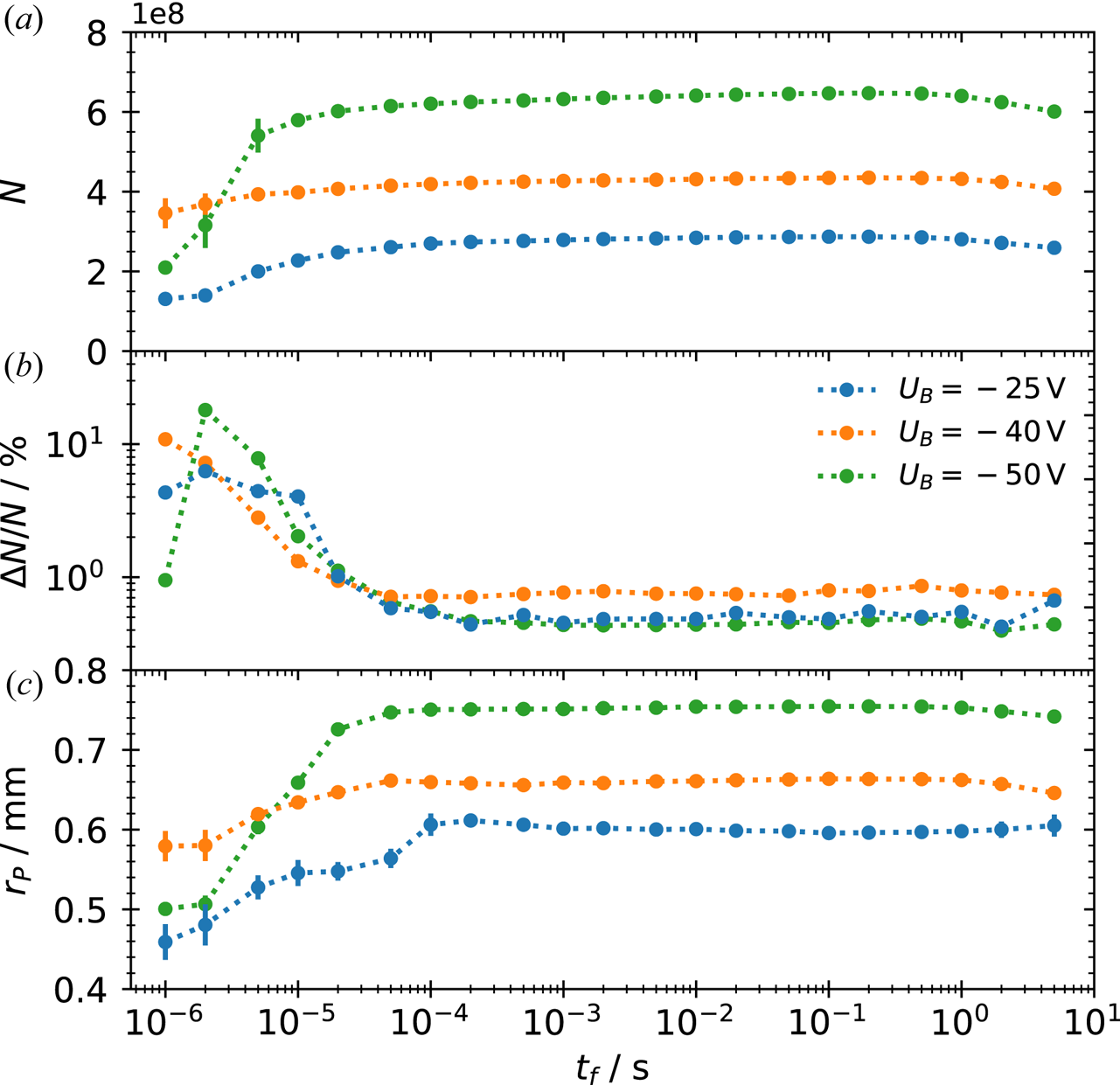
Figure 4. (a) Number of particles $N$ , (b) shot-to-shot deviation ${\rm \Delta} N/N$
 , (c) plasma radius $r_P$
 versus the fill time $t_{f}$
 , for plasma creation in the master cell with the LaB$_{6}$
 crystal at bias voltages of $-$
 25 V (blue), $-$
 40 V (orange) and $-$
 50 V (green). The dotted lines are added to guide the eye. Each data point is the average of 100 repetitions, with the error bars given by the standard deviation. Beyond approximately 1 ms the error bars are smaller than the data symbols.
These plasmas have a length of ${\approx }90$ mm and central density of $2.75\times 10^9$
 to $3.98\times 10^9$
 cm$^{-3}$
 . Initially their 2-D distribution can be approximated by a 2-D Gaussian function. This indicates a rather high plasma temperature $T_P$
 which may be related to the high emitter bias. However, measurements of the plasma temperature in other high-field experiments (Eggleston et al. Reference Eggleston, Driscoll, Beck, Hyatt and Malmberg1992; Beck, Fajans & Malmberg Reference Beck, Fajans and Malmberg1996) show that through cyclotron cooling in the magnetic field (O'Neil Reference O'Neil1980) the plasma quickly (${\approx }1$
 s) cools down to corresponding energies of $k_{B}T_P \le 1$
 eV, where $k_{B}$
 denotes the Boltzmann constant, and evolves to a flat-top profile. The temperature diagnostic used currently has a lower limit of $k_{B}T_P \approx 1$
 eV. The trap is at room temperature, and no increased radial transport compared with the prototype master cell was observed that would hint to additional sources of plasma heating. Therefore, due to the continuous cyclotron cooling in the 3.1 T field the actual expected plasma temperature at late times (10 to 100 s) should be close to room temperature, i.e., $k_{B}T_P \approx 0.03$
 eV.
eV.
6. Limits on confinement
During confinement studies in the prototype master cell, a charge loss was observed for holding times ${>}100$ s (Singer et al. Reference Singer, König, Stoneking, Steinbrunner, Danielson, Schweikhard and Pedersen2021). The plasma was well confined i.e. on axis the confinement potential was large compared with the plasma potential $(|\phi_{C} \,(r=0)| \gg |\phi_{P}\, (r=0)|)$
 , and the plasma radius small compared with the wall radius $(r_{W}\gg r_{P})$
 . The particle loss remained unexplained and it was speculated that electron attachment to neutral background hydrogen atoms could be the reason for it (Kabantsev, Thompson & Driscoll Reference Kabantsev, Thompson and Driscoll2018).
To test this hypothesis, the confinement measurement is repeated. A plasma is created in the master cell between M1 and M5, the residual diocotron mode damped, and then the plasma is confined for increasing hold times $t_{hold}$ up to 66.7 min. In contrast to the previous study, a two-stage ejection scheme similar to the ejection of cooling electrons from antimatter traps (Fajans & Surko Reference Fajans and Surko2020) is utilized for these experiments. In the first stage, electrons are ejected by briefly ($10\,\mathrm {\mu }$
 s) lowering the confinement potential on the screen side. Since electrons are light and fast compared with any molecules or atoms, they escape the trap quickly while the heavier particles remain. In the second stage, after an additional delay of 3 ms, which is related to the decay time of the phosphor screen, the confinement potential is lowered for 100 ms so the remaining particles can escape the trap.
The outcome of this measurement is shown in figure 5. The integrated pulse, which is proportional to the dumped charge, is measured with the RC-circuit and plotted versus hold time. The two-stage ejection makes two distinct, negatively charged particle populations visible: the first population (red dots) is constant at the beginning and starts to decrease exponentially for $t_{hold}>100$ s. The second population (blue dots) stays constant near zero and starts to grow on the same time scale as the first decreases. The sum of charge stays constant (black crosses) within the error margin. This supports the assumption that the electrons are not lost during the confinement but rather attach to background neutrals. This creates a second population of confined charged particles which cannot be distinguished in the 2-D profiles nor measured with a single ejection.
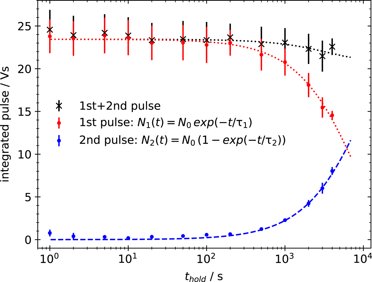
Figure 5. Measurement of the confined charge within the master cell with the RC-circuit (Vs) for increasing hold times $t_{hold}$ (s). Two ejections are performed: one short ($10\,\mathrm {\mu }$
 s) pulsed ejection (red dots) and after 3 ms a second, long (100 ms) ejection (blue dots). The red dotted and the blue dashed line are exponential decay or increase fits to the respective data. The black crosses represent the sum of both ejections. An exponential decay fit (dotted black line) yields a charge-confinement time of the total charge of 8.6 h.
A detailed analysis of the dump signals further supports this assumption. The first population arrives nearly instantaneously with the dump pulse. After $1\,\mathrm {\mu }$ s the signal reaches a maximum and plateaus, meaning that all fast particles have arrived at the screen. The dump signal for the second population starts $7\,\mathrm {\mu }$
 s after the ejection, and the signal does not plateau until after $50\,\mathrm {\mu }$
 s, suggesting at a larger mass and a much broader distribution in the velocity space. Due to the small flight path to the screen, it is not possible to determine the mass(es) of the ions that produce the second signal. Mass spectrometric analysis of the residual gas shows signals corresponding to H$_{2}^{+}$
 , O$^+$
 , HO$^+$
 , H$_2$
 O$^+$
O$^+$ and N$_{2}^{+}$
 with water being the most dominant.
For further investigation of the confinement an exponential decay following the formula $N_{1}(t)=N_{0}\exp (-t/\tau _{1})$ is fit to the decreasing population (red dotted line), and an increasing rate equation $N_{2}(t)=N_{0} (1-\exp (-t/\tau _{2}))$
 to the growing one (blue dashed line). They yield time constants of $\tau _{1}=7809(288)$
 s and $\tau _{2}=9772(370)$
 ms, indicating an electron confinement decay time above 1 h. If the exponential decay fit is applied to the sum of both pulses the resulting time constant $\tau _{3}=31049.52(2)$
 s yields an actual charge-confinement time of 8.6 h within the master cell.
When working with positrons the attachment to background neutrals, followed by annihilation with electrons, could become a considerable loss factor if the pressure in the confinement region exceeds $10^{-8}$ mbar. However, the confinement is more likely to be limited by general annihilation with free electrons in the trap, or positronium formation through charge-exchange, three-body or radiative recombination (Stoneking et al. Reference Stoneking, Pedersen, Helander, Chen, Hergenhahn, Stenson, Fiksel, von der Linden, Saitoh and Surko2020). Also, there will be different confinement limits in the storage cells. Due to their smaller radius, irregularities on the electrode's surfaces are much closer to the plasma. These would have a deleterious effect on the plasma, likely providing a torque against the plasma rotation, reducing the canonical angular momentum, and leading to radial transport (Kriesel Reference Kriesel2000). Hence, the ultimate confinement limit in the storage cells is expected to be set by expansion.
7. Competing diocotron motion
An experimental cycle which transfers and traps particles in the off-axis cells usually consists of five steps. 1. After the plasma is prepared in the master cell, the $m=1$ diocotron mode is autoresonantly excited, displacing the plasma from the axis of symmetry. 2. When the plasma reaches the centre position of the off-axis cell the confinement potential at M1 and TE is quickly grounded. 3. The plasma expands into the off-axis storage cell until it reaches the potential barrier applied to either electrode ${\rm S}_{1.1}$
 or ${\rm S}_{3.1}$
 . After the transfer time $t_{T}$
 , the confinement potential to M1 and TE is reapplied, ‘cutting out’ a part of the plasma which extends from the master into the storage cell. 4. The remaining plasma in the master cell is usually dumped onto the screen. However, it is also possible to damp the diocotron mode, bringing the plasma back on axis for further use. 5. During this time, and potentially longer, the transferred plasma is confined in the off-axis cell before its dumped and diagnosed with the phosphor screen.
In the master cell, the radial plasma motion is dominated by the diocotron drift dynamics. When expanded over a large-diameter trap, where it is displaced from the axis of symmetry, and a small diameter one (during step 3.), this dynamics changes. Intuitively, one could think that the motion in the large-diameter traps dominates, and the plasma further spirals around its centre of symmetry, driving it into the off-axis cell's wall. However, being extended over both traps results in an overlap of two contributions to the diocotron motion. Due to the different wall radii the plasma dynamics is determined by two $E\times B$ -drifts in the electric field E of the image charges at the surface of the electrodes and the trap's magnetic field B. Since the electrons bounce very fast ($f_{\mathrm {bounce}} \sim {\rm MHz}$
 ) between both plasma ends, individual particles experience a bounce-average contribution to the diocotron drift dynamics. The resulting orbit is elliptical and slightly displaced from the centre of the off-axis cell. This behaviour, called ‘competing diocotron drift motion’, was discovered in the first generation MCT (Hurst et al. Reference Hurst, Danielson, Baker and Surko2014).
Figure 6 shows a measurement of competing diocotron motion for a plasma expanded into storage cell ${\rm S}_{1}$ . At $t_{T}=0$
 s, M1 and TE are grounded so that the plasma can expand into the storage cell. The plasma is held in this expanded state for $t_{T}$
 before it is dumped onto the phosphor screen without further confinement. Figure 6(a) shows the $xy$
 -plane with the red dashed line marking the wall of the storage cell. The storage cell is centred at $(x,y)=(0,0)$
 mm (red star) and the centre of the master cell is oriented in the direction of $(x,y)=(-6,-6)$
 mm. Here, $t_{T}$
 is scanned from $10\,\mathrm {\mu }$
 s to 1 ms in steps of ${\rm \Delta} t_{T}=10\,\mathrm {\mu }$
 s. For increasing $t_{T}$
 the plasma rotates clockwise. The complete plasma profiles (the density colour coded) are visualized for the first $140\,\mathrm {\mu }$
 s and the estimated centres (black dots) for the whole measurement, except for the first five measurements.
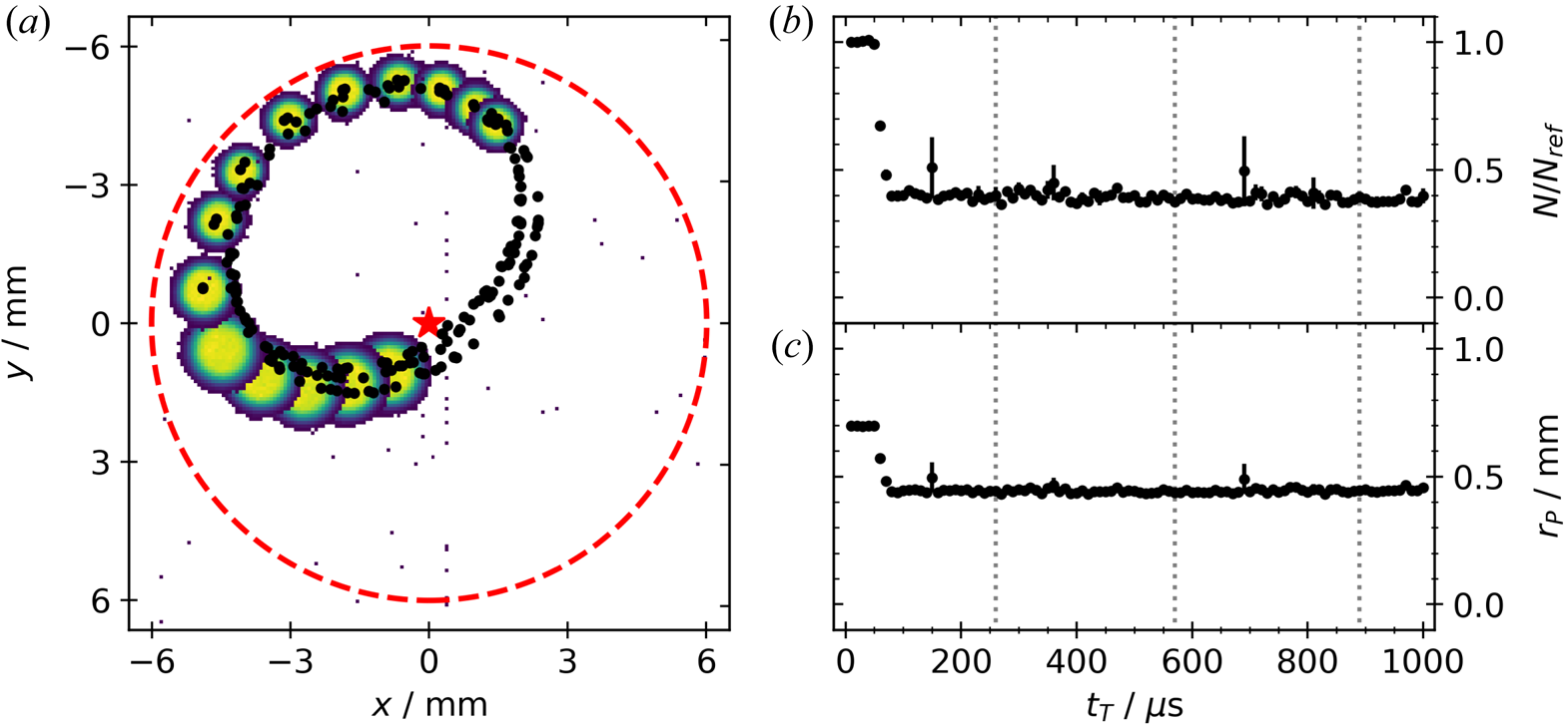
Figure 6. Competing diocotron motion for a plasma which is expanded over the master cell and storage cell ${\rm S}_{1}$ . (a) Shows the $xy$
 -plane with the red dashed line representing the wall of the storage cell, and the master cell's centre in direction of $(-6,-6)$
 . The yellow–green spots are the measured 2-D plasma profiles and the black dots the plasma centres. For the profiles $3/4$
 of a revolution ($140\,\mathrm {\mu }$
 s) around the centre of the ellipse is visualized. The plasma rotates clockwise. The two graphs on the right show (b) the normalized particle number $N/N_{{\rm ref}}$
 and (c) plasma radius $r_{P}$
 (mm) over the transfer time $t_{T}$
 ($\mathrm {\mu }$
 s). The period of the motion is indicated by the dotted vertical lines in (b,c).
After quarter revolution ($t_{T} \approx 50\,\mathrm {\mu }$ s) the plasma reaches the storage-cell wall, nearly touching it. But the increasing electric field of the image charges at the inner surface of ${\rm S}_{1}$
 overwhelms the contribution of the master cell, leading to a resulting diocotron motion pointing away from the wall. Since a fraction of the plasmas charge is lost before the image fields can alter the resulting diocotron motion and due to the conservation of angular momentum (O'Neil Reference O'Neil1980) the plasma shrinks substantially in this time. However, after $t_{T}\approx 80\,\mathrm {\mu }$
 s there is no further charge loss. The resulting elliptical diocotron motion is shifted into the direction of the master-cell centre and continues until the plasma expands radially to the wall (on time scales not depicted here).
The right half of figure 6 shows for the same measurement (b) the normalized particle number $N/N_{{\rm ref}}$ , and (c) plasma radius $r_{P}$
 versus $t_{T}$
 . At $t_{T} \approx 50\,\mathrm {\mu }$
 s the plasma gets close to the wall. A substantial particle loss of approximately $60\,\%$
 is measured while simultaneously the plasma shrinks from 0.7 to 0.45 mm within the next $30\,\mathrm {\mu }$
 s, confirming that the change in the radial profile is due to a change of the total charge. Afterwards both parameters are stable. The dotted black lines indicate one revolution around the centre of the ellipse. One revolution takes approximately $260\,\mathrm {\mu }$
 s which corresponds to a frequency of approximately 3.85 kHz. The motion is stable for at least $3.5$
 turns. However, other measurements indicate a stable plasma revolution for longer periods ($t_{T} \ge 100$
 ms) until the plasma begins to radially expand. This behaviour is qualitatively the same in storage cell ${\rm S}_{3}$
 .
.
The diocotron dynamics during the transfer described by Hurst et al. (Reference Hurst, Danielson, Baker and Surko2019) shows a similar behaviour where the plasma gets close to the wall, losing a large fraction of the total charge. This can be explained by the competing contributions to the diocotron motion. The different lengths of the plasma in the master cell $L_{{\rm MC}} \approx 170$ mm and storage cell $L_{{\rm SC}} \approx 90$
 mm mean that a particle spends nearly twice as much time in the master cell. Therefore, the contribution of the master cell is larger and dominates the motion through the first $50\,\mathrm {\mu }$
 s. Only very close to the storage cell's wall, when the field of the image charges increases drastically, can the storage cell's contribution compete with the one from the master cell. When the plasma now loses particles, this changes its charge per unit length $N/l_{P}$
 (and to a small degree $l_{p}$
 as well). Due to the diocotron frequency being proportional e.g. $f_{0} \approx N/l_{P}$
 , this shifts both constituents of the motion to a stable state with a fixed centre of motion and no further particle loss.
When working with positrons, particles loss during transfer must be avoided. There are three ways to achieve this: first, the length of the master cell can be reduced, or the storage-cell length increased, reducing the master cell's contribution to the resulting motion. At some length ratio $L_{{\rm MC}}/L_{{\rm SC}}$ the diocotron motion in the storage cell will dominate and the resulting trajectory will be closer to a circle around the centre of the storage cell. However, it is not possible to increase the storage-cell length in the present set-up, and the master-cell length would have to be decreased until plasmas are only trapped between M1 and M3, which deteriorates the autoresonant diocotron excitation.
Second, one could reduce the length of the plasma in the master cell after the displacement, right before initiating the transfer. However, this would shift the resulting frequency and needs a more complicated frequency monitoring to ground M1 and TE at the right time to start the transfer. Also, this should happen adiabatically on time scales (${\approx }10$ to 100 ms) which would probably lead to radial expansion of the plasma prior to the transfer.
The third option uses static fields in the storage cell during the transfer. These fields, covering only a part of the solid angle using the segmented electrodes, can counter the contribution of the master cell to the resulting diocotron dynamics. This ansatz will be further explored in a future publication. However, for a reproducible plasma transfer it is necessary to centre the plasma in the storage cell and mitigate the losses. For this reason, the following section presents measurements of the plasma transfer where the amplitude of the competing diocotron motion is reduced substantially, and the plasma is centred in the off-axis cell. This mitigates losses due to the competing diocotron motion.
8. On- and off-axis transfer
Now, the protocol described above is used to explore the achievable transfer rates. For comparison a reference cycle is included for each measurement, measuring the displaced plasmas before initiating the off-axis transfer; obtaining the electron number $N_{\mathrm {ref}}$ and density $n_{0, \mathrm {ref}}$
 while monitoring long-time fluctuations. The transferred plasmas are measured for increasing times $t_{T}$
 when they are extended over both traps and compared with the displaced reference plasmas. For the on-axis case the transfer is initiated without displacing the plasma from the master cell's axis of symmetry. In all three cases the plasmas are centred in the storage cells during the transport, as mentioned above, and confined between M1 and TE and ${\rm S}_{1.1}$
 /${\rm S}_{2.1}$
 /${\rm S}_{3.1}$
 for 3 ms prior to the measurement on the screen.
Figure 7 shows (a) the normalized transfer rate $N/N_{\mathrm {ref}}$ , (b) plasma radius $r_{P}$
 and (c) normalized central density $n_{0}/n_{0,\mathrm {ref}}$
 versus the transfer time $t_T$
 . The off-axis traps ${\rm S}_{1}$
 (blue) and ${\rm S}_{3}$
 (orange) are compared with the on-axis case ${\rm S}_{2}$
 (green). The dotted lines for the first and last plots are added to guide the eye. In the first plot the black dotted line marks a transfer efficiency of $50\,\%$
 . For the plasma radius an exponential fit with $r_{P}(t_{T})= r_{P}(t_{T}=0\,{\rm s})\exp (t/\tau _{r}) +\mathrm {offset}$
 is applied to the data to determine the radial expansion time scale $\tau _{r}$
 for each case. The results are represented by the dotted lines for the respective data set and the time constants are given in the legend. Since the radial expansion is only to a certain extent exponential, the points for the fit include times up to 50 ms for ${\rm S}_{1}$
 , to 100 ms for ${\rm S}_{3}$
 and up to 2000 ms for ${\rm S}_{2}$
 .
.
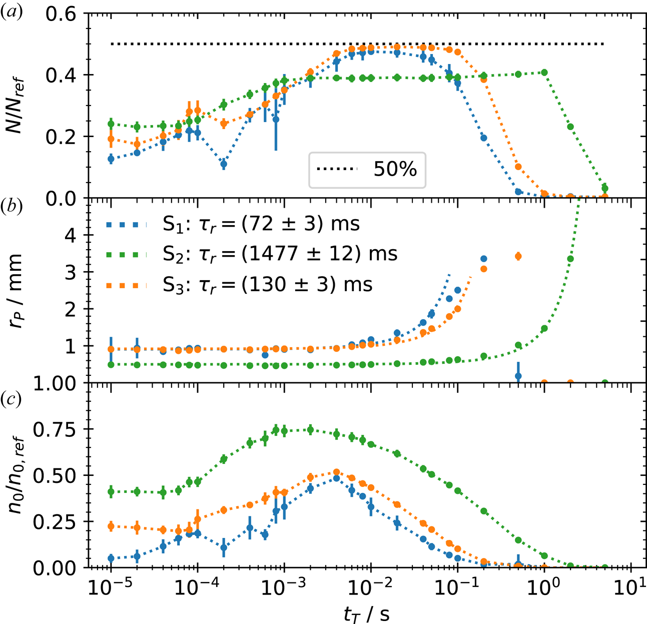
Figure 7. Transferred plasmas measured in the off-axis cells ${\rm S}_{1}$ (blue) and ${\rm S}_{3}$
 (orange) as well as on-axis in ${\rm S}_{2}$
 (green). The (a) normalized transferred particles $N/N_{\mathrm {ref}}$
 , (b) plasma radius $r_P$
 (mm) and (c) the normalized central density $n_{0}/n_{0,\mathrm {ref}}$
 are given for the transfer time $t_T$
 (s). The dotted lines in the first and third plots are given to guide the eyes. The black dotted line in (a) marks a transfer rate of $50\,\%$
 . The dotted lines in (b) are exponential fits to determine the expansion rates $\tau _r$
 which are given in the legend.
For all three storage cells the amount of transferred charge increases within the first milliseconds after M1 and TE are grounded at $t_{T}=0$ s, and then plateaus. On axis, it takes 0.8 ms to reach the plateau, while, off axis, it takes a magnitude longer. The normalized density shows a similar behaviour. At first it stays constant until at $t_{T} \sim 0.01$
 ms it quickly increases and reaches a maximum which coincides with the beginning of the plateau region in the normalized charge. Through this early state the plasma radius stays constant for all three cases. Off axis it is a bit larger for the displaced plasma than for the on-axis case, due to the radial expansion from the autoresonant excitation (Baker et al. Reference Baker, Danielson, Hurst and Surko2015). At $t_{T} \sim {\rm ms}$
 the plasma starts to expand radially. On axis it expands with a time constant of $\tau _{r}=1477(12)$
 ms. Off axis the expansion happens with time constants of $\tau _{r}=130(3)$
 ms for ${\rm S}_{3}$
 and $\tau _{r}=72(3)$
 ms for ${\rm S}_{1}$
 . These are approximately a factor of 10 and 20 shorter compared with ${\rm S}_{2}$
 . The difference between the on- and off-axis expansion is related to the broken symmetry in the master cell when the plasma is displaced off axis. However, the difference between the two off-axis cases is not fully understood. It is likely due to small manufacturing variances which add some asymmetry induced transport (Kabantsev et al. Reference Kabantsev, Yu, Lynch and Driscoll2003) that is stronger in ${\rm S}_{1}$
 than in ${\rm S}_{3}$
 . On axis, the density decrease starts earlier than the radial expansion, while off axis both coincide. In all three cases the plasma begins to lose particles after the exponential radial expansion phase ends i.e. after 50 ms for ${\rm S}_{1}$
 , 100 ms for ${\rm S}_{3}$
 and 2000 ms for ${\rm S}_{2}$
 .
.
With this simple transfer scheme, it is possible to transfer $50\,\%$ of the initial particles to the off-axis cells without large radial expansion. However, the maximum on-axis transfer was only $40\,\%$
 . This decreased efficiency can be explained by the confinement fields both plasmas experience and the corresponding plasma lengths. When a confinement potential of $\phi _{C}=-300$
 V is applied to M5, the plasma experiences an actual potential of $\phi _{C} (r=0)=-187$
 V on axis in the master cell. When the plasma is displaced to $70\,\%$
 of the wall radius the potential it experiences due to M5 increases to $\phi _{C} (r/r_{W} =0.7)=-245$
 V. This reduces the length of the plasma in the master cell since the point where $\phi _{C} (r/r_{W} =0.7) \sim \phi _{P}$
 moves into the direction of the storage cells. As a result, a larger fraction of charge is transferred to the off-axis storage cell.
9. On- and off-axis confinement
To comparably test the storage-cell confinement, a fixed transfer time of 5 ms was chosen and subsequently the plasmas were held for increasing hold times $t_{\mathrm {hold}}$ without further plasma manipulation separately in each cell. Figure 8 shows the resulting normalized charge signal $N/N_{0}$
 in storage cells ${\rm S}_{1}$
 (a), ${\rm S}_{2}$
 (b) and ${\rm S}_{3}$
 (c) versus $t_{\mathrm {hold}}$
 . The decrease of the charge signal can be described by an exponential function $N(t)=N_{0}\exp (-t/\tau ) +\mathrm {offset}$
 . This function was fitted to the data (dashed lines) to determine the decay constant $\tau$
 and the reference number of particles $N_{0}$
 for the normalization. The respective decay constants are given in the legend.
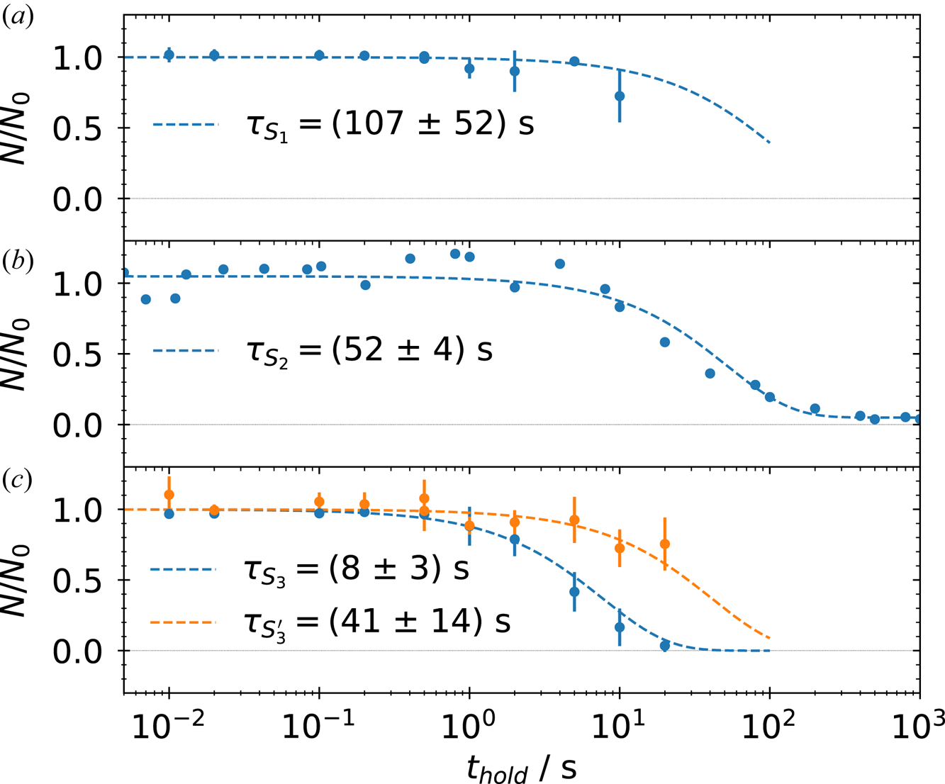
Figure 8. Normalized electron number (blue dots) for increasing hold times within ${\rm S}_{1}$ (a), ${\rm S}_{2}$
 (b) and ${\rm S}_{3}$
 (c). For ${\rm S}_{3}$
 the measurement was repeated (see text) with an excluded segmented electrode (orange dots). The dashed lines are exponential fits to the data with the respected decay constants shown in the legend.
The charge signal stays approximately constant up to 2 s in ${\rm S}_{1}$ and ${\rm S}_{2}$
 , which is reflected by the similarity of the time constants $\tau _{{\rm S}_{1}}=107(52)$
 s and $\tau _{{\rm S}_{2}}=52(4)$
 s within the range of uncertainty. However, in ${\rm S}_{3}$
 with the decrease starting already at 0.2 s, and a 5 times lower time constant of $\tau _{{\rm S}_{3}}=8(3)$
 s, a reduced confinement ability is observed. This is likely caused by the eight-fold segmented electrode of ${\rm S}_{3}$
 . During the assembly the proper alignment of these parts of the electrode were difficult and could be now a source for asymmetries. To test this hypothesis, the segmented electrode of ${\rm S}_{3}$
 was excluded from the confinement region by applying the confinement potential to it as well and repeating the measurement. The result is shown in orange in figure 8(c). With the segmented electrode excluded the charge decrease begins at 2 to 5 s, and the time constant increases to $\tau _{{\rm S}_{3}'}=41(14)$
 s, making the confinement comparable to those in ${\rm S}_{1}$
 and ${\rm S}_{2}$
 . This shows that the eight-fold segmented electrode is the likely cause for the increased transport in ${\rm S}_{3}$
 . It introduces an asymmetry which produces an additional drag on the plasma and drives radial transport (O'Neil Reference O'Neil1980). However, by excluding the segmented electrode the plasma length and trapped number of electrons are also reduced, which should be considered as well since both are relevant for determining the radial transport (Kriesel Reference Kriesel2000).
Since the plasma is expanding on an orbit displaced from the centre, and the detailed density evolution in the off-axis cells has not yet been studied, these factors are not yet deconvolved from purely asymmetry driven transport. Also, it needs to be confirmed whether the confinement in the storage cells will be limited by electrons attaching to background neutrals as observed in the master cell. In any case, the achieved confinement time is long enough for further plasma manipulation in the storage cells: the damping of the residual $m=1$ diocotron mode, followed by the application of a rotating electric field to prevent radial expansion and compress the plasma (Danielson, Weber & Surko Reference Danielson, Weber and Surko2006).
The demonstrated confinement is already much longer than the time needed to transfer electrons into one storage cell. Thus, it is possible to perform two transfers, one following the other, into separate off-axis cells by using the same scheme as described earlier. First, a plasma is transferred to ${\rm S}_{3}$ . Afterwards, a new plasma is prepared in the master cell and then the same protocol (but with a different phase) is used to transfer it into ${\rm S}_{1}$
 . After the ${\rm S}_{1}$
 plasma is confined for 3 ms the whole content of the storage-cell stack is dumped onto the phosphor screen. This is visualized in figure 9. It shows the $xy$
 -plane of the screen. The large black dashed circle marks the inner wall of the master cell and the smaller circles mark the wall radius of the three storage cells. Both off-axis cells hold a plasma. The density of the plasma transported to ${\rm S}_{3}$
 is lower than the one trapped in ${\rm S}_{1}$
 . This is due to the serial nature of the experiment and thus the plasma in ${\rm S}_{3}$
 has evolved for ${\sim }1.5$
 s at the time of the measurement whereas the plasma in ${\rm S}_{1}$
 was only confined for 3 ms. Also, ${\rm S}_{3.5}$
 was used for the confinement which slightly decreased the number of transferred charges and plasma length. This experiment is the first to demonstrate that two different plasmas can be consecutively transferred to two different off-axis traps and be trapped simultaneously, a key step in the development of the MCT concept.

Figure 9. Phosphor screen image with the signals of two plasmas from the off-axis cells ${\rm S}_{3}$ and ${\rm S}_{1}$
 . First, a plasma was transferred to ${\rm S}_{3}$
 (upper left) and then to ${\rm S}_{1}$
 (lower right), while the first plasma was still confined in ${\rm S}_{3}$
 . Afterwards, both plasmas were ejected simultaneously. The large black dashed circle represents the wall of the master cell and the three smaller ones the wall of the storage cells.
10. Summary and outlook
A second prototype MCT has been constructed to address open questions relating to the MCT concept. Construction and operation of the new trap has been detailed and the commissioning process described. The phosphor screen is calibrated by exciting the diocotron motion until the plasma reaches the wall, projecting it onto the screen. With the presented alignment technique, it is possible to align the storage cell with an accuracy of ${\rm \Delta} \zeta _{1}=1(3)$ mdeg and the whole trap to ${\rm \Delta} \zeta _{2}=3(5)$
 mdeg relative to the background magnetic field. Positions of the off-axis cells are obtained using the autoresonant excitation followed by a controlled axial expansion in the direction of the cells. Plasma creation with a lanthanum hexaboride emitter has been studied and found to be a reliable source to create highly reproducible (${\rm \Delta} N/N\le 0.5\,\%$
 ) electron plasmas. Also, the total charge confinement is found to be 8.6 h, whereas the electron confinement on long time scales (${>}1$
 min), limited by electron attachment to background neutrals, has been verified.
The competing diocotron drift motion during the time the plasma is extended over the master and storage cells is studied and compared with previous measurements. This motion can result in a non-negligible particle loss and possible ways to mitigate these losses are discussed. Plasmas have been transferred to the on- and off-axis cells using a simple transfer method. The maximum transfer efficiency off axis was found to be $50\,\%$ whereas the maximum in the on-axis case was approximately $40\,\%$
 , with the difference understood to be due to the variation in the trapped plasma length. Confinement experiments have been performed in all three storage cells and the confinement times are observed to be suitable for the next set of experiments. The confinement is found to be similar on and off axis, and to be sufficient to demonstrate the first consecutive plasma transfer and confinement in two different off-axis cells.
The next experiments will include tests of techniques to increase the transfer rate and to develop a more advanced transfer protocol as well as one for the off-axis ejection, where the plasmas are brought back on axis in the master cell to form pulses for the transfer to the future pair-plasma experiments. Further, stacking of multiple plasmas in the off-axis cells to create large plasma space charges and their off-axis confinement will be studied to achieve the targeted particle numbers for the pair-plasma experiments envisioned.
Acknowledgements
We wish to thank Dr. G. Marx for his technical assistance and help with the MCT design, and the APEX collaboration for the helpful discussions of the experiments.
Editor Francesco Califano thanks the referees for their advice in evaluating this article.
Funding
This work was supported by the Deutsche Forschungsgemeinschaft (M.S., S.K., grant numbers SCHW 401/23-1, HU 978/16-1 and PE 2655/1-1); the European Research Council (ERC) under the European Union's Horizon 2020 research and innovation program (M.S., T.S.P., grant number 741322); the U.S. Department of Energy (J.R.D., grant number DE-SC0016532); and the Helmholtz Association (E.V.S., grant number VH-NG-1430).
Data availability statement
The data that support the findings of this study are available from the corresponding author upon reasonable request.
Declaration of interests
The authors report no conflict of interest.


 Open access