

Geographic information systems (GIS) are software tools used for organizing, manipulating, analyzing, and visualizing spatial data (Conolly and Lake Reference Conolly and Lake2006). Once a niche element in archaeology, GIS are now among the most common applications of computing in the field, and a familiar work component in the management of historic and archaeological heritage (McCoy and Ladefoged Reference McCoy and Ladefoged2009). Technological developments in the collection, storage, and retrieval of geospatial data have resulted in the steady growth of datasets available for researchers, inviting increasingly sophisticated analyses of spatial processes and phenomena (Bevan Reference Bevan2015; McCoy Reference McCoy2017).
Given its history and present ubiquity, it is no surprise that GIS in archaeology has also been a subject of recurrent critique. Developments in the management and visualization of spatial data have flourished, but archaeologists have struggled with interpretive applications or using GIS to characterize causal dynamics (Aldenderfer Reference Aldenderfer, Costopoulos and Lake2010:61; Hu Reference Hu2012; Lock and Pouncett Reference Lock and Pouncett2017). Some have suggested that broadening GIS approaches beyond strict representation would help further the goals of archaeological interpretation, while many propose adapting a more explicit modeling ethos. Verhagen (Reference Verhagen, Siart, Forbriger and Bubenzer2018:21 sensu Hacιgüzeller Reference Hacιgüzeller2012) for example, recommends an “eclecticism” in spatial approaches to encourage the study and comparison of multiple pasts. Similarly, Llobera (Reference Llobera2012:505) argues that rather than using GIS to reconstruct past landscapes, practitioners would benefit from engaging with an “archaeology of potentials,” where possible scenarios are explored and compared by way of middle-range “scaffolding models.”
Dynamic simulation approaches, particularly agent-based models (ABMs), are often used as a way of dealing with “potentials” in archaeology (e.g. Cucart-Mora et al. Reference Cucart-Mora, Lozano and Fernández-López de Pablo2018; Gravel-Miguel and Wren Reference Gravel-Miguel and Wren2018; Riris Reference Riris2018). The agents in an ABM represent individual entities in a system that act according to a set of predetermined rules. Agents can use their current state along with information gathered from their environment or from other agents to change their behavior in different contexts. The primary advantage of this kind of modeling is that it allows the user to observe the emergence of macro-level (population level) regularities through the interactions of individuals over time (Epstein Reference Epstein2006).
These two approaches—GIS- and agent-based modeling—are highly complementary for engaging with an archaeology of potentials. For example, studying mapped trade routes using a GIS-based least-cost path analysis will show the difference between the “easiest” route from point A to point B and the actual route discovered in the archaeological record (e.g., Frachetti et al. Reference Frachetti, Evan Smith, Traub and Williams2017; White and Barber Reference White and Barber2012). To investigate a potential trading process that might have resulted in the transport following a certain path, a simulation technique (e.g., ABM) can be employed. The “artificial” trading routes generated by the ABM can then be compared with both the actual and the “ideal” (least-cost) routes to examine how the simulated processes influence path behavior and whether they could be responsible for the observed paths (e.g. Gravel-Miguel and Wren Reference Gravel-Miguel and Wren2018). In this example, GIS-based analysis is used to detect and describe patterns in data, while ABMs act as theoretical scaffolding to investigate processes that might have led to these patterns.
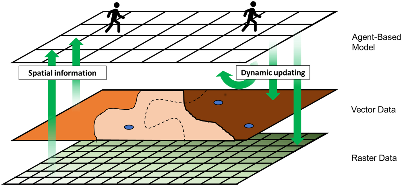
ABM and GIS are different software tools that can be used to address different kinds of questions, but they share many methodological elements that situate them under the broader umbrella of geocomputation. For example, ABMs commonly feature a gridded world of attribute-carrying “patches” which operate in much the same manner as raster-like data in GIS (and can also represent polygon-like data through rasterization). Agents themselves are attribute-carrying, (usually) zero-dimensional objects similar to point-like GIS data. A time step in an ABM, then, is like a set of rule-based calculations in GIS that produce updated values for feature attributes. From a GIS-oriented perspective, the agent-based model could be thought of as a layer, but one that is capable of drawing on raster and vector datasets and transforming both itself and the underlying data (Figure 1). The repeated use of updating to represent the passage of time is a primary difference in the usual applications of ABM and GIS methods, but the fundamental operations and relationships underlying this process are conceptually similar.

FIGURE 1. Relationships between agent-based model and integrated geographic information system.
Joining the two approaches brings together the precision and spatial data standards of GIS with the explicit representation of time and individual autonomy in ABM. This combination is frequently advocated in other sectors (e.g., Alghais and Pullar Reference Alghais and Pullar2018; Crooks and Wise Reference Crooks and Wise2013; Guo et al. Reference Guo, Ren, Wang, Kang, Cai, Yan and Liu2008), but there are few resources for doing so within archaeological literature. This how-to article will demonstrate the integration of GIS with ABM, with the aim of improving methodological capacity for theory building in archaeology.
SOME PRACTICAL CONSIDERATIONS
In archaeology, the relationships among objects within three dimensions and through time gives us context from which our interpretations are derived. Simulating social processes within a geospatial framework is appealing, then, because of the potential to connect models to real-world entities recorded as GIS data. At the same time, focusing on a specific geographic setting or distribution of data adds additional complexity to a model and can reduce its applicability beyond the case study at hand.
In model building of any kind, there is always a trade-off between realism, generality, and precision. For example, the most common output of GIS in archaeology is maps, which are models of one or more aspects of reality. For a map, maximizing detail (precision and realism) often means limiting the area being depicted (generality) to avoid significant loss of readability. The same is true in an ABM: while it is possible simulate anything, trying to simulate too many processes at once makes a model difficult to interpret and therefore less useful (Bullock Reference Bullock2014).
Making strategic simplifications when representing real-world phenomena can improve our understanding of key relationships in a system or process. But this leaves in question whether variables not included in the model have any substantial effect on the process being modeled. Before integrating GIS and ABM, it is worthwhile to consider whether the geographic relationships between entities are important features of the model. The following questions can help to clarify this:
• Is the research question dependent on place-specific geographic conditions? There are many questions that are not dependent on a specific spatial context, even if the processes in a specific case have geographic components. For example, a study investigating the role of spatial foresight in forager movement patterns has a geographic component but may cover a wide range of potential conditions (Wren et al. Reference Wren, Xue, Costopoulos and Burke2014). In such cases, the model may need “some” geography rather than place-specific conditions, and the geographic setting could be considered a variable where any map could be used (e.g., Ullah and Bergin Reference Ullah, Bergin, White and Surface-Evans2012). Alternatively, stochastic landscape generation might be more appropriate to model different kinds of geographic conditions (see Perry and O'Sullivan Reference Perry and O'Sullivan2018 for an example). Some questions, though, are not easily extricated from their geographic setting. For example, models used to explore routes of hominin dispersals out of Africa (Mithen and Reed Reference Mithen and Reed2002) or land use in Neolithic Mediterranean contexts (Barton et al. Reference Barton, Ullah, Heimsath, Michael Barton, Ullah and Heimsath2015) may be dependent on specific terrestrial and marine environments or spatially explicit biophysical processes. In such cases, it may be necessary to include place-specific geospatial information.
• Are the target outcomes partly or wholly spatial measurements? Model-based studies often aim to produce outcomes that resemble real-world targets (Godfrey-Smith Reference Godfrey-Smith2006). In some cases, these will not have an obvious spatial definition, or they can be generalized in ordinal terms such as “more or less dense.” In such instances, it may be more advantageous to model abstract processes that produce these more broadly defined categories (e.g., Crema Reference Crema2014; Davies et al. Reference Davies, Holdaway and Fanning2016). But sometimes, targets are defined by more precise geospatial patterning; for example, a population gradient along a particular geographic transect (Romanowska et al. Reference Romanowska, Gamble, Bullock and Sturt2017) or the regional distribution of ritual site characteristics (Crabtree et al. Reference Crabtree, Kyle Bocinsky, Hooper, Ryan and Kohler2017). These situations may require more detailed spatial information to be included in, or produced by, the simulation.
A MOTIVATING EXAMPLE
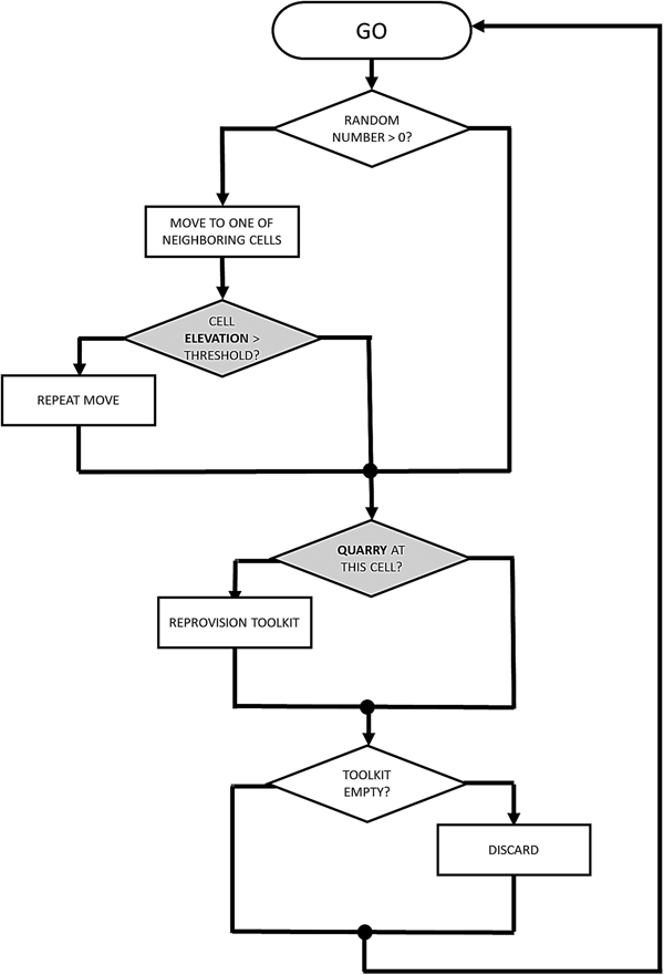
Imagine that our research problem is focused on understanding relationships between movement and stone artifact discard in a specific geographic context. Our GIS data might include a set of spatial points representing stone quarries and a rasterized digital elevation model of an island. Here, we present a model based on Brantingham's (Reference Brantingham2003) neutral model of procurement, in which an agent moves randomly from patch to patch in the landscape and discards artefacts at each stop (Figure 2). If the agent comes into contact with a quarry, the agent fills its toolkit. In the present model, the agent makes multiple moves in places where elevation is greater than a given threshold, simulating more frequent or rapid movement at higher elevations. For the sake of the exercise, it is presumed that higher elevations would be less attractive, and that movements would therefore be more rapid, carrying the expectation that there would be less frequent discard than at lower elevations.

FIGURE 2. Diagram of proposed agent-based model components drawing on GIS data in shaded gray.
The example model draws on vector and raster datasets, and, in a simple way, can be used to assess how terrain might affect mobility and, by extension, frequency of discard. The interplay between the behavioral rules and the geography of the island are of interest, so values such as the number of time steps (ticks), the agents’ toolkit capacity, the threshold determining “high” elevation, and a coefficient for more frequent movement applied to those higher elevations are included as tuneable model parameters with which to explore their effects on model outcomes, producing a range of potential pasts and their archaeological outcomes. Ultimately, the utility of this or any model depends on whether it sufficiently represents the theoretical historical process under examination. If not, then further elaboration of the model and its behavioral rules may be needed in order to make it work for a particular research question.
A primary barrier to the combined use of GIS and ABM in archaeology is the computational skills needed. Limited learning opportunities exist within the discipline, requiring self-teaching for many practitioners (Davies and Romanowska Reference Davies and Romanowska2018). The remainder of this article provides an introduction on combining ABM and GIS for an archaeological study, drawing on code components from the above example. A more thorough tutorial is given as Supplemental Text, while the code and data files are available from an online repository. The average time it takes to complete the tutorial is two hours.
GETTING STARTED
There are many options for combining ABMs with GIS, including free and/or open-source options. Well-known packages used by social science researchers include Repast (North et al. Reference North, Collier, Ozik, Tatara, Macal, Bragen and Sydelko2013), NetLogo (Wilensky Reference Wilensky1999), GAMA (Grignard et al. Reference Grignard, Taillandier, Gaudou, Vo, Huynh and Drogoul2013), and Mason (Luke et al. Reference Luke, Cioffi-Revilla, Panait, Sullivan and Balan2005), with published comparisons available (Crooks and Castle Reference Crooks, Castle, Heppenstall, Crooks, See and Batty2012; Railsback et al. Reference Railsback, Lytinen and Jackson2006). Commonly used programming languages such as Python or Java have ABM libraries that can also be made capable of interfacing with GIS data. Most of these have user communities either independently or through online forums such as Stack Exchange. Some proprietary options, such as AnyLogic, also have GIS capability and offer the added benefit of on-call technical support (Borshchev Reference Borshchev, Brailsford, Churilov and Dangerfield2014). On the other end of the spectrum, ESRI software extends to the Agent Analyst package (derived from Repast), which can be used to build ABMs within the proprietary ArcGIS environment (Johnston Reference Johnston2013). Similarly, the Python-based MML-Lite software, developed for addressing questions related to long-term landscape ecodynamics, operates as an add-on to the popular open-source GRASS GIS software (Barton et al. Reference Barton, Ullah, Heimsath, Michael Barton, Ullah and Heimsath2015).
For this demonstration, NetLogo modeling software was chosen because it (a) has a built-in GIS extension; (b) can handle common spatial data types used by archaeologists (e.g., shapefiles and ASCII rasters); (c) is one of the easier ABM software packages to learn (Railsback et al. Reference Railsback, Lytinen and Jackson2006); (d) has good documentation and an active user community; (e) is a stand-alone platform requiring no additional software or system configurations to operate; and (f) is free to download. Although many of the principles discussed here can be transferred to other ABM platforms, the commands used herein will be specific to NetLogo. The supplemental tutorial was created using NetLogo 6.0.2, the most recent version at the time of writing, and the code can be found in a Github repository. References to NetLogo code will be printed in Courier New font. Comments, or lines of code that are not run as part of the program, are preceded by a semicolon (;) in NetLogo.
The NetLogo platform possesses several of the basic characteristics of a GIS, in the sense that it keeps track of spatial data in a systematic way, and it can be used to create visualizations of spatial data (Figure 3). The easiest way to access GIS data from NetLogo is through the GIS extension, which gives the programmer a set of commands for working with vector and raster datasets. As is done in the example model, this can be added using the following code:
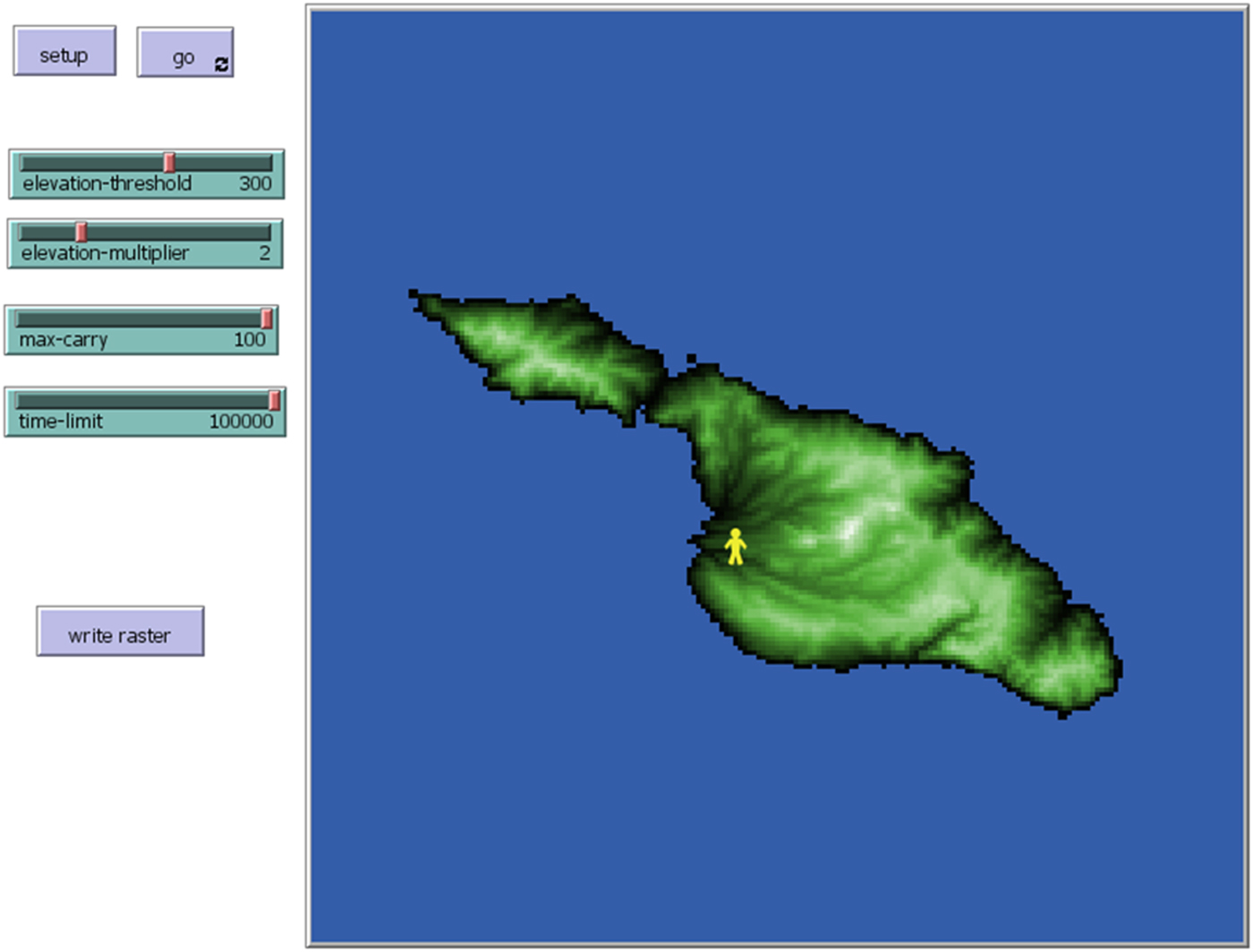
FIGURE 3. NetLogo model interface featuring imported elevation data (see supplemental tutorial for details).
Example:
;access NetLogo GIS extension
extensions [ gis ]
NetLogo is similar to other ABM platforms in that it revolves around computational agents (known by the default name “turtles”) following a set of behavioural rules in an environment of gridded cells (known by the default name “patches”). Both agents and grid cells can possess characteristics (turtle-owned and patch-owned variables, e.g., age, wealth, presence/absence of resources) that may change over time, typically through interactions among agents, among grid cells, and between agents and grid cells. The NetLogo user interface is divided into Interface, Info, and Code tabs, which are used for interacting, documenting, and programming, respectively. For the sake of space (pun intended), NetLogo programming basics will not be discussed in any detail. Romanowska et al. (Reference Romanowska, Crabtree, Harris and Davies2019) provide an archaeology-specific introduction, and there are a number of textbooks (O'Sullivan and Perry Reference O'Sullivan and Perry2013; Railsback and Grimm Reference Railsback and Grimm2012) and online tutorials that deal with NetLogo programming directly.
GIS DATASET AND COORDINATE SYSTEM OPERATIONS
In order for NetLogo to use external GIS data, the data must be loaded and interpreted in terms of the NetLogo world, including the coordinate system being used to describe the data. First, GIS data used in NetLogo need to be imported to a named variable in the NetLogo world. This is accomplished using the gis:load-dataset command, which opens a filename specified as a string. Within the example code, both the elevation dataset (raster) and the quarries (point shapefile) are loaded using this command:
Example:
; load elevation data from ascii raster
set elevation gis:load-dataset “dem.asc”
; load lithic source data from point shapefile
set quarries gis:load-dataset “quarries.shp”
Next, the extents, or “envelopes,” of the GIS data need to be described in terms of the NetLogo world window. The gis:envelope-of command extracts the extent of a saved GIS dataset as a list of minimum and maximum x and y values, while the gis:world-envelope command does the same for the NetLogo patch world. The gis:set-world-envelope and gis:set-world-envelope-ds commands map the extent of a GIS dataset onto the NetLogo patch world, the latter permitting different scales on the x and y axes. The elevation dataset is used to define the world envelope in the example model:
Example:
; resize the world to fit the patch-elevation data
gis:set-world-envelope gis:envelope-of elevation
Geographic coordinate systems can be used in NetLogo using the gis:load-coordinate-system command, and the coordinate system can be changed using gis:set-coordinate-system. To use gis:load-coordinate-system, geographic or projected coordinate systems in Well-Known Text (WKT) format need to be saved as .prj files in the same location as the GIS dataset being used (and, by default, this should be wherever the model's .nlogo file is saved). If a .prj file is associated with a data file, NetLogo will default to using that file and will continue to use that coordinate system for subsequent data unless otherwise specified. Alternatively, gis:set-coordinate-system can be used by converting WKT descriptions into NetLogo lists. A list of supported projected coordinate systems can be found in the NetLogo User Manual. Once again, this is drawn from the elevation data:
Example:
; loads coordinate system using the .prj file from the ; elevation
; data
gis:load-coordinate-system “dem.prj”
INTERACTING WITH GIS DATA
There are two ways to make imported spatial data available to agents in NetLogo: by using GIS data to create or alter entities within the NetLogo world (i.e., agents or patches), or by using the GIS extension within agent or patch behavioral rules. Shapefiles are imported into NetLogo as a set of nested lists that contain the individual features within the dataset, each of their properties, their spatial locations, etc. Agents and patches can interact with these data through a set of commands that allow the user to establish whether a topological relationship holds between two entities (e.g., vector features, patches, turtles). The gis:intersects? command reports true if any part of one entity overlaps with another, while gis:contained-by? and gis:contains? only report true if the entirety of one entity is inside the bounds of another. In the example, this is used by agents who reprovision their toolkits when in proximity of a quarry:
Example:
; if a turtle shares an intersecting relationship ; with the shapefile dataset, it proceeds to the
; “reprovision-toolkit” procedure
ask turtles [
if gis:intersects? quarries self [
reprovision-toolkit
]
]
Another set of commands is used for accessing aspects of the GIS data such as vertices, features, properties (attributes), centroids, and locations. The gis:vertex-list-of and gis:feature-list-of commands return a nested list of vertices or feature properties, respectively, of a GIS dataset. When given a single feature and a property name, the gis:property-value command will give the property value for that feature (for example, the ID of a polygon). The gis:centroid-of returns x and y coordinates for the geographic center of a feature in GIS space, while gis:location-of gives the NetLogo location of a GIS point (or vertex or centroid). The example model uses these when the agent is reprovisioning, identifying the ID number of the nearest quarry, which will be used to associate items added to the toolkit with that quarry:
Example:
; stores the ID of a nearby quarry (the “first” ID value ; of a list of features contained by the patch where
; the turtle is located) as a temporary variable t
; located) as a temporary variable t
let t gis:property-value first (filter [ q -> gis:contained-by? q patch-here] (gis:feature-list-of quarries)) “ID”
There are two different commands that can be used to translate a raster dataset into a NetLogo variable. The gis:raster-sample command transmits a single value from the raster at a given point, while gis:apply-raster applies the raster values to patches across the NetLogo world. In the example model, the patches sample values from the underlying raster in order to determine their own elevation:
Example:
; each patch sets its “patch-elevation” variable to
; a value extracted from the “elevation” GIS dataset
; at the patch's centroid
ask patches [
set patch-elevation gis:raster-sample elevation self
]
There are additional commands in the NetLogo GIS extension that, for the sake of space, are not covered in this brief overview. These include commands used to find maximum and minimum values of a GIS dataset, subsetting GIS features with specific values, exporting NetLogo agents as shapefiles, etc. A full list of commands can be found in the Extensions section of the NetLogo Manual. Another extension allows NetLogo to be interfaced with the R statistical computing platform (Thiele and Grimm Reference Thiele and Grimm2010), which has packages that can be used to perform many common techniques in spatial analysis, as well as some more rarefied ones (Bivand et al. Reference Bivand, Pebesma and Gomez-Rubio2013).
AVOIDING COMMON ERRORS
As with all software, user errors can cause problems with both NetLogo and the GIS extension. This can be frustrating for beginning users, as the cause of error messages may be unclear. For example:
Extension exception: error parsing number
error while observer running GIS:LOAD-DATASET
called by procedure LOAD-RASTER
called by Command Center
This indicates that a symbol in a GIS dataset cannot be read by NetLogo. To avoid this error, raster data used in NetLogo should be in ASCII (.asc) or ESRI grid (.grd) file types, and vector data should be ESRI shapefiles (.shp). In addition, commas should not be used in numerical values, header terms in raster files need to be separated from their values by single spaces, and files should be free from word-processor formatting such as indents and carriage returns. Many of these issues can be fixed by opening the file with a basic text editor and making the necessary changes using a search-and-replace function.
Errors also occur when simulations exceed the heap space, the memory available for objects and calculations. This can be changed to handle larger projects (see NetLogo Manual FAQ), but it is limited by the RAM available on the machine. It may be more appropriate in these cases to resize or resample the spatial data as long as this does not adversely affect the spatial relationships in the model or limit the size of the NetLogo world window (described in Supplemental Text).
This is by no means an exhaustive list of potential errors or solutions. If an error occurs that is not listed above, the NetLogo Users Group is a useful place to ask questions.
CONCLUDING THOUGHTS
This brief demonstration provides a basic overview for integrating GIS and ABM, but does so without providing more basic information about coding in NetLogo. The tutorials in this series, as well as those in the NetLogo User Manual, are a good place to start. Further instruction with model exemplars can be found in Wilensky and Rand (Reference Wilensky and Rand2015), O'Sullivan and Perry (Reference O'Sullivan and Perry2013), and Railsback and Grimm (Reference Railsback and Grimm2012).
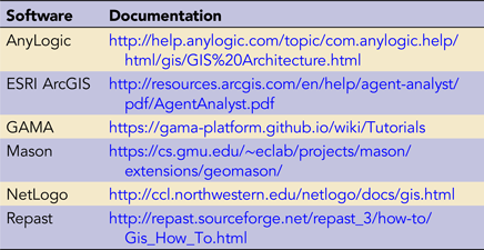
As noted above, NetLogo is not the only software solution for integrating GIS and ABM, and users may find other solutions more suited to their needs. Different options vary to some extent both in their capabilities and in terms of their online documentation and tutorials. Table 1 gives a selection of platforms for which documentation was easily located at the time of publication.
TABLE 1. Software Platforms and Links to Documentation for Integrating GIS and ABM
The context of archaeological data is primarily spatial, and spatial relationships continue to play an important role in archaeological interpretation. As spatial data collected by archaeologists and others continues to expand and become more accessible, opportunities to draw on these datasets to evaluate and reevaulate our understanding of the past are multiplying (Bevan Reference Bevan2015). At the same time, a great deal of uncertainty remains around historical processes that could have given rise to archaeological patterning, spatial or otherwise. Considering material records in terms of an archaeology of potentials, one in which the archaeological record of the present is the emergent outcome of historically and geographically contingent processes, will aid in characterizing that uncertainty. Such an approach benefits from the affordances of an eclectic range of geocomputational methods (Verhagen Reference Verhagen, Siart, Forbriger and Bubenzer2018). Combining GIS and ABM offers archaeologists working in both academic and professional spheres a toolkit for investigating spatial processes that contribute to the dynamics of potential pasts and their material residues in the present.
Supplemental Material
For supplemental material accompanying this article, visit https://doi.org/10.1017/aap.2019.5
Supplemental Text. Tutorial 2: Combining Geographic Information Systems and Agent-Based Models in Archaeology
Acknowledgements
This manuscript and tutorial have evolved out of a number of ABM workshops courses we have given, and we extend our thanks to the many participants who have helped us to develop these materials over the years. The authors declare no conflicts of interest. IR received funding from the European Research Council (ERC) under the European Union's Horizon 2020 Research and Innovation programme (grant agreement no. ERC-2013-ADG340828). SC acknowledges support by NSF Graduate Research Fellowship DGE-080667, an NSF GROW fellowship, and a Chateaubriand Fellowship. BD acknowledges support as a postdoctoral fellow from NSF under CNHS-1826666. We thank three anonymous reviewers for comments that benefited the manuscript. We also thank Colin Wren for providing detailed consideration of the manuscript and tutorial materials.
Data Availability Statement
Software used in the tutorial is open access and open source. Code and data files are available from a Zenodo repository. The “dem.asc” dataset used in this example is an ASCII raster extracted from tile n34w119 of the USGS National Elevation Dataset, centered on Santa Catalina Island, California. The “quarries.shp” dataset is a shapefile of simulated quarry locations.