


Nomenclature
- Symbols
Connotation
- F
Assembly feature
- U
Network nodes
- L
Assembly level
- Z
The number of nodes $ \delta $
Assembly feature deviation
- T
Transfer entropy
- p
Probability density
- H
Information entropy
- e
Information entropy weight
- $ \lambda $
Kendall coefficient weight
- C
Degree centrality
- $ \psi $
Contribution


1.0 Introduction
Complex thin-walled structure products such as aircraft have the characteristics of poor stiffness, high assembly accuracy, complex structures and many assembly levels. Deformation recovery of thin-walled parts, part manufacturing errors and installation positioning errors will cause assembly deviations and then lead to assembly over-tolerance easily [Reference Zhang, Wang and Tan1–Reference Liu, An and Wang3]. If the deviation transfer model can’t be established to diagnose the key deviation sources that affect the assembly quality, the aircraft assembly quality can’t be improved efficiently and at a low cost. Therefore, it is the key for the deviation source diagnosis to build a deviation transfer model.
In recent years, many universities and researchers have conducted research on the calculation and analysis of deviation transfer. For instance, Chase et al. proposed the mathematical model of transfer and accumulation by regarding assembly parts as rigid bodies [Reference Chase, Gao and Magleby4, Reference Chase, Magleby and Gao5]. Based on the rigid body assumption of assembly parts, Mantriparagada et al. applied a mathematical model of assembly deviation transfer and accumulation to the calculation and analysis of multi-station assembly deviations [Reference Mantripragada and Whitney6]. Zhang et al. achieved the identification of key influencing factors by combining the complex networks and entropy weight method [Reference Zhang, Wang and Deng7]. McKenna et al. first presented a variation propagation model for overconstrained assemblies and develops a novel modeling method to connect variations with production costs [Reference Mckenna, Jin and Murphy8]. Considering the deformation of thin-walled parts during assembly, Falgarone et al. used the finite element method to calculate assembly deviations of thin-walled parts [Reference Falgarone, Thiébaut and Coloos9]. Zhang et al. applied the finite element method to the deformation analysis of the riveting assembly of thin-walled parts [Reference Zhang, Cheng and Li10–Reference Aman, Cheraghi and Krishna12]. Simulation modeling and large-scale calculation are needed by the finite element method. This method has the disadvantages of long cycles and high costs. It is difficult to meet the tolerance design and product analysis of complex structures such as aircraft. To make full use of assembly deviation data, Chen Hui et al. proposed a statistical analysis method for thin-walled parts, based on normal distribution [Reference Chen, Tan and Wang13]. High-precision digital measuring equipment has been successfully applied to all stages of aircraft assembly, such as laser tracker [Reference Liu, Luo and Tan14–Reference Lei and Zheng16]. Real and reliable data of aircraft assembly deviation transfer and accumulation can be measured by using high-precision digital measurement equipment. It is of great significance for finding the key deviation sources that affect the assembly quality to mine the information contained in the data [Reference Zhu, Den and Huo17, Reference Liu, Tian and Geng18].
Small batch production is often used in large complex thin-walled structures products, such as aircraft. Small batch production will lead to a small sample size of detection data and has many assembly features. The detection data of assembly deviation has the characteristics of high dimension and small sample size. The detection data of assembly deviation can’t be calculated and analysed by traditional statistical methods. In addition, the deviation transfer between deviation sources and assembly parts has the characteristics of nonlinearity and strong coupling. Therefore, it is difficult to calculate the assembly deviation by building assembly dimension chains. Transfer entropy can not only describe the information quantity between systems but also describe the directivity and the dynamic nonlinearity of information transfer [Reference Ye, Liu and He19–Reference Liu, Yu and Liang21]. In addition, it has no requirement for the sample size. Topological structures of complex systems can be described by complex networks [Reference Wu, Wang and Gan22–Reference Zhang and Lyu24]. It is suitable for aircraft product assembly which has a large number of assembly parts and complex structures. Taking the assembly deviation of aircraft complex thin-walled structures as the object, a key deviation sources diagnosis method of complex structures is proposed based on complex networks and weighted transfer entropy. Firstly, the complex network is used to describe the topological relationship of product structure. Then, the transfer entropy is used to quantify the deviation transfer relationship in complex networks. Secondly, considering the difference in the importance of each node in the complex network, the information entropy and Kendall coefficient are used to obtain the weighted transfer entropy. Furthermore, the contribution between nodes is obtained. Finally, from the perspective of the entire complex network structure, the depth-first traversal algorithm is used to obtain the deviation transfer path, and the degree centrality theory is used to define the global importance of each node, which the total contribution of each deviation source to assembly deviation of the product is calculated.
2.0 Assembly deviation transfer complex networks of complex thin-walled structures
2.1 Assembly feature tree
During the assembly process of complex thin-walled structures, assembly feature surfaces contact each other. With the contact, assembly feature deviations will be transferred to the next level of assembly parts. Eventually, it forms the deviation of complex thin-walled structures. Different from error, assembly deviation refers to the difference between the theoretical position and the actual position of the assembly part. The assembly deviation of the assembly feature contains the geometric relationship and deviation data.
In view of this, according to the assembly process information of complex thin-walled structures, assembly part features are obtained and assembly sequences are defined. The assembly feature tree is constructed, as shown in Fig. 1.

Figure 1. Assembly feature tree of complex thin-walled structures.
2.2 Complex networks of assembly deviation transfer
A lot of information can be described by the assembly feature tree, including the assembly levels, assembly relationships between parts and the feature information extracted from each assembly part. However, it can’t obtain the importance of each assembly feature. Nodes and connection edges of complex network theory agree with part features and deviation information transfer in the assembly process. From network topology, the importance of each node can be described by degree centrality theory. It makes the key deviation source diagnosis more accurate.
Therefore, complex networks are introduced to describe the deviation transfer process. Network nodes represent assembly features, such as the position of the assembly hole. Connection edges represent assembly relationships between features. Complex networks of assembly deviation transfer are constructed. Complex networks of assembly deviation transfer are denoted as $G = \left\{ {U,E,W} \right\}$
. Where U represents a set of network nodes, namely, assembly features of each part. E represents a set of connection edges of complex networks, namely, assembly relations between assembly features. W represents the deviation transfer relationships between nodes, namely, the size of deviation information transfer between assembly features. In addition, Z represents the number of nodes. Z×Z Adjacency matrix M represents the assembling condition of each node in deviation transfer networks. Among them,
$G = \left\{ {U,E,W} \right\}$
. Where U represents a set of network nodes, namely, assembly features of each part. E represents a set of connection edges of complex networks, namely, assembly relations between assembly features. W represents the deviation transfer relationships between nodes, namely, the size of deviation information transfer between assembly features. In addition, Z represents the number of nodes. Z×Z Adjacency matrix M represents the assembling condition of each node in deviation transfer networks. Among them, $M\!\left( {i,j} \right) = 1$
represents that node
$M\!\left( {i,j} \right) = 1$
represents that node ${U_i}$
and node
${U_i}$
and node ${U_j}$
have an assembly relationship, otherwise it is 0.
${U_j}$
have an assembly relationship, otherwise it is 0.
3.0 Assembly deviation transfer based on weighted transfer entropy
3.1 Quantitative description of assembly deviation transfer based on transfer entropy
The assembly feature deviation of the node $U_{{L_\alpha }}^\mu $
is denoted as
$U_{{L_\alpha }}^\mu $
is denoted as ${\boldsymbol{\delta}_{U_{{L_\alpha }}^\mu }} = \left\{ {{\delta _{U_{{L_\alpha }}^{\mu 1}}},{\delta _{U_{{L_\alpha }}^{\mu 2}}}, \cdots ,{\delta _{U_{{L_\alpha }}^{\mu n}}}} \right\}$
in the L
α
level of the deviation transfer networks. The assembly feature deviation of the node
${\boldsymbol{\delta}_{U_{{L_\alpha }}^\mu }} = \left\{ {{\delta _{U_{{L_\alpha }}^{\mu 1}}},{\delta _{U_{{L_\alpha }}^{\mu 2}}}, \cdots ,{\delta _{U_{{L_\alpha }}^{\mu n}}}} \right\}$
in the L
α
level of the deviation transfer networks. The assembly feature deviation of the node $U_{{L_\beta }}^\nu $
is denoted as
$U_{{L_\beta }}^\nu $
is denoted as ${\boldsymbol{\delta} _{U_{{L_\beta }}^\nu }} = \left\{ {{\delta _{U_{{L_\beta }}^{\nu 1}}},{\delta _{U_{{L_\beta }}^{\nu 2}}}, \cdots ,{\delta _{U_{{L_\beta }}^{\nu n}}}} \right\}$
in the
${\boldsymbol{\delta} _{U_{{L_\beta }}^\nu }} = \left\{ {{\delta _{U_{{L_\beta }}^{\nu 1}}},{\delta _{U_{{L_\beta }}^{\nu 2}}}, \cdots ,{\delta _{U_{{L_\beta }}^{\nu n}}}} \right\}$
in the $L_{\beta}$
level, where n denotes the assembly number of times.
$L_{\beta}$
level, where n denotes the assembly number of times.
Transfer entropy can quantify the information transfer between variables. Transfer entropy ${T_{U_{{L_\alpha }}^\mu \to U_{{L_\beta }}^\nu }}$
is used to quantify the deviation transfer relationship between
${T_{U_{{L_\alpha }}^\mu \to U_{{L_\beta }}^\nu }}$
is used to quantify the deviation transfer relationship between $U_{{L_\alpha }}^\mu $
and
$U_{{L_\alpha }}^\mu $
and $U_{{L_\beta }}^\nu $
.
$U_{{L_\beta }}^\nu $
.
 \begin{equation}{T_{U_{{L_\alpha }}^\mu \to U_{{L_\beta }}^\nu }} = \sum {p\!\left( {{\delta _{U_{{L_\alpha }}^{\mu (n + 1)}}},{\delta _{U_{{L_\alpha }}^{\mu n}}}^{({\tau _1})},{\delta _{U_{{L_\beta }}^{\nu n}}}^{({\tau _2})}} \right)} \log \frac{{p\!\left( {{\delta _{U_{{L_\alpha }}^{\mu (n + 1)}}}\left| {{\delta _{U_{{L_\alpha }}^{\mu n}}}^{({\tau _1})},{\delta _{U_{{L_\beta }}^{\nu n}}}^{({\tau _2})}} \right.} \right)}}{{p\!\left( {{\delta _{U_{{L_\alpha }}^{\mu (n + 1)}}}\left| {{\delta _{U_{{L_\alpha }}^{\mu n}}}^{({\tau _1})}} \right.} \right)}},\end{equation}
where $p\!\left( {{\delta _{U_{{L_\alpha }}^{\mu (n + 1)}}},{\delta _{U_{{L_\alpha }}^{\mu n}}}^{({\tau _1})},{\delta _{U_{{L_\beta }}^{\nu n}}}^{({\tau _2})}} \right)$
denotes the joint probability density of
$p\!\left( {{\delta _{U_{{L_\alpha }}^{\mu (n + 1)}}},{\delta _{U_{{L_\alpha }}^{\mu n}}}^{({\tau _1})},{\delta _{U_{{L_\beta }}^{\nu n}}}^{({\tau _2})}} \right)$
denotes the joint probability density of ${\delta _{U_{{L_\alpha }}^{\mu (n + 1)}}}$
,
${\delta _{U_{{L_\alpha }}^{\mu (n + 1)}}}$
, ${\delta _{U_{{L_\alpha }}^{\mu n}}}^{({\tau _1})}$
and
${\delta _{U_{{L_\alpha }}^{\mu n}}}^{({\tau _1})}$
and ${\delta _{U_{{L_\beta }}^{\nu n}}}^{({\tau _2})}$
respectively.
${\delta _{U_{{L_\beta }}^{\nu n}}}^{({\tau _2})}$
respectively. $p\!\left( {{\delta _{U_{{L_\alpha }}^{\mu (n + 1)}}}\left| {{\delta _{U_{{L_\alpha }}^{\mu n}}}^{({\tau _1})}} \right.} \right)$
denotes the conditional probability density.
$p\!\left( {{\delta _{U_{{L_\alpha }}^{\mu (n + 1)}}}\left| {{\delta _{U_{{L_\alpha }}^{\mu n}}}^{({\tau _1})}} \right.} \right)$
denotes the conditional probability density. $p\!\left( {{\delta _{U_{{L_\alpha }}^{\mu (n + 1)}}}\left| {{\delta _{U_{{L_\alpha }}^{\mu n}}}^{({\tau _1})},{\delta _{U_{{L_\beta }}^{\nu n}}}^{({\tau _2})}} \right.} \right)$
denotes the conditional probability density function of
$p\!\left( {{\delta _{U_{{L_\alpha }}^{\mu (n + 1)}}}\left| {{\delta _{U_{{L_\alpha }}^{\mu n}}}^{({\tau _1})},{\delta _{U_{{L_\beta }}^{\nu n}}}^{({\tau _2})}} \right.} \right)$
denotes the conditional probability density function of ${\delta _{U_{{L_\alpha }}^{\mu (n + 1)}}}$
.
${\delta _{U_{{L_\alpha }}^{\mu (n + 1)}}}$
. $\tau_1$
and
$\tau_1$
and $\tau_2$
denote the power of
$\tau_2$
denote the power of ${\delta _{U_{{L_\alpha }}^{\mu n}}}$
and
${\delta _{U_{{L_\alpha }}^{\mu n}}}$
and ${\delta _{U_{{L_\beta }}^{\nu n}}}$
respectively.
${\delta _{U_{{L_\beta }}^{\nu n}}}$
respectively.
To avoid the calculation of a high-dimensional probability density function, let ${\tau _1} = {\tau _2} = 1$
. Equation (1) is rewritten as
${\tau _1} = {\tau _2} = 1$
. Equation (1) is rewritten as
 \begin{equation}{T_{U_{{L_\alpha }}^\mu \to U_{{L_\beta }}^\nu }} = \sum {p\!\left( {{\delta _{U_{{L_\alpha }}^{\mu (n + 1)}}},{\delta _{U_{{L_\alpha }}^{\mu n}}},{\delta _{U_{{L_\beta }}^{\nu n}}}} \right)} \log \frac{{p\!\left( {{\delta _{U_{{L_\alpha }}^{\mu (n + 1)}}}\left| {{\delta _{U_{{L_\alpha }}^{\mu n}}},{\delta _{U_{{L_\beta }}^{\nu n}}}} \right.} \right)}}{{p\!\left( {{\delta _{U_{{L_\alpha }}^{\mu (n + 1)}}}\left| {{\delta _{U_{{L_\alpha }}^{\mu n}}}} \right.} \right)}}.\end{equation}
According to the calculation formula of conditional probability
 \begin{equation}p\!\left( {{\delta _{U_{{L_\alpha }}^{\mu (n + 1)}}}\left| {{\delta _{U_{{L_\alpha }}^{\mu n}}}} \right.} \right) = p{\left( {{\delta _{U_{{L_\alpha }}^{\mu (n + 1)}}}{\delta _{U_{{L_\alpha }}^{\mu n}}}} \right)} \Big/ {p\!\left( {{\delta _{U_{{L_\alpha }}^{\mu n}}}} \right)}.\end{equation}
As shown in Equation (2), effective probability density estimation is needed to calculate ${T_{U_{{L_\alpha }}^\mu \to U_{{L_\beta }}^\nu }}$
. Prior knowledge of data distribution is not needed for kernel density estimation. Any assumed data distribution is not included in kernel density estimation. It meets the characteristics of aircraft small batch production. Therefore, kernel density estimation is introduced to define the probability density of assembly feature deviations in the L
α
level.
${T_{U_{{L_\alpha }}^\mu \to U_{{L_\beta }}^\nu }}$
. Prior knowledge of data distribution is not needed for kernel density estimation. Any assumed data distribution is not included in kernel density estimation. It meets the characteristics of aircraft small batch production. Therefore, kernel density estimation is introduced to define the probability density of assembly feature deviations in the L
α
level.
 \begin{equation}p\!\left( {{\delta _{U_{{L_\alpha }}^{\mu x}}}} \right) = \frac{{\rm{1}}}{{n - 2h - 1}}\sum\limits_{y = 1}^n {K\!\left( {\varepsilon - \left\| {{\delta _{U_{{L_\alpha }}^{\mu x}}} - {\delta _{U_{{L_\alpha }}^{\mu y}}}} \right\|} \right)} ,\end{equation}
where h is the Theiler window size. It is used to eliminate deviations from kernel density estimation. $\varepsilon$
denotes the bandwidth of the kernel density function.
$\varepsilon$
denotes the bandwidth of the kernel density function. $K\!\left( \cdot \right)$
denotes the unit step function.
$K\!\left( \cdot \right)$
denotes the unit step function.
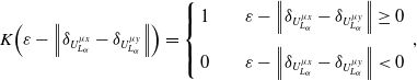 \begin{align}K\!\left( {\varepsilon - \left\| {{\delta _{U_{{L_\alpha }}^{\mu x}}} - {\delta _{U_{{L_\alpha }}^{\mu y}}}} \right\|} \right) = \left\{ \begin{array}{l}1{\rm{ }}\qquad\varepsilon - \left\| {{\delta _{U_{{L_\alpha }}^{\mu x}}} - {\delta _{U_{{L_\alpha }}^{\mu y}}}} \right\| \geq 0\\[1em]0\qquad{\rm{ }}\varepsilon - \left\| {{\delta _{U_{{L_\alpha }}^{\mu x}}} - {\delta _{U_{{L_\alpha }}^{\mu y}}}} \right\| \lt 0\end{array} \right.,\end{align}
where $\left\| {{\delta _{U_{{L_\alpha }}^{\mu x}}} - {\delta _{U_{{L_\alpha }}^{\mu y}}}} \right\|$
is the distance norm of assembly feature deviations.
$\left\| {{\delta _{U_{{L_\alpha }}^{\mu x}}} - {\delta _{U_{{L_\alpha }}^{\mu y}}}} \right\|$
is the distance norm of assembly feature deviations.
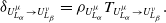
Similarly, the probability density of assembly feature deviations is defined in the $L_{\beta}$
level. Incorporating Equations (2)–(5), transfer entropy between assembly feature deviations can be obtained.
$L_{\beta}$
level. Incorporating Equations (2)–(5), transfer entropy between assembly feature deviations can be obtained.
 \begin{equation}{T_{U_{{L_\alpha }}^\mu \to U_{{L_\beta }}^\nu }} = \frac{1}{n}\sum {\log \frac{{p\!\left( {{\delta _{U_{{L_\alpha }}^{\mu (n + 1)}}},{\delta _{U_{{L_\alpha }}^{\mu n}}},{\delta _{U_{{L_\beta }}^{\nu n}}}} \right)p\!\left( {{\delta _{U_{{L_\alpha }}^{\mu n}}}} \right)}}{{p\!\left( {{\delta _{U_{{L_\alpha }}^{\mu n}}},{\delta _{U_{{L_\beta }}^{\nu n}}}} \right)p\!\left( {{\delta _{U_{{L_\alpha }}^{\mu (n + 1)}}},{\delta _{U_{{L_\alpha }}^{\mu n}}}} \right)}}} .\end{equation}
3.2 Node importance empowerment
The difference of importance from each node fails to be considered by transfer entropy. The deviation information quantity of nodes can be measured by information entropy. The correlation between nodes can be measured by the Kendall coefficient. Therefore, the information entropy and Kendall coefficient are introduced to objectively quantify the node importance from two different aspects. One is the size of the information quantity, the other is the correlation degree between nodes. It overcomes shortcomings of the node importance empowerment based on experience.
-
Deviation Matrix A of each node
\begin{equation*}\textbf{A} = \left[ {\begin{array}{*{20}{c}}{\delta _{{U_1}}^1}&& {\delta _{{U_2}}^{\rm{1}}}&& \cdots &&{\delta _{{U_Z}}^{\rm{1}}}\\ \vdots && \vdots && \cdots && \vdots \\{\delta _{{U_1}}^k} && {\delta _{{U_2}}^k} && \cdots && {\delta _{{U_Z}}^k}\\ \vdots && \vdots && \cdots && \vdots \\{\delta _{{U_1}}^n} && {\delta _{{U_2}}^n} && \cdots && {\delta _{{U_Z}}^n}\end{array}} \right],\end{equation*}
where Z denotes the number of complex network nodes.
$\delta _{{U_Z}}^k$
denotes deviation detection data of nodes. -
Proportion matrix P of deviation detection data
\begin{equation*}\textbf{P} = \left[ {\begin{array}{*{20}{c}}{P^1_{{U_1}}}&& {P^1_{{U_2}}}&& \cdots && {P^1_{{U_Z}}}\\ \vdots && \vdots&& \cdots&& \vdots \\{P^k_{{U_1}}}&& {P^k_{{U_2}}}&& \cdots && {P^k_{{U_Z}}}\\ \vdots && \vdots && \cdots && \vdots \\{P^n_{{U_1}}}&& {P^n_{{U_2}}} && \cdots && {P^n_{{U_Z}}}\end{array}} \right],\end{equation*}
where
$P_{{U_Z}}^k$
denotes the proportion of deviation detection data of the k-th assembly in all number of assemblies.(7)
\begin{equation}P_{{U_Z}}^k = \frac{{\delta _{{U_Z}}^k}}{{\sum\limits_{k = 1}^n {\delta _{{U_Z}}^k} }}.\end{equation}
-
Calculation of node information entropy
${H_{{U_i}}}$
.(8)
\begin{equation}{H_{{U_i}}} = - \frac{1}{{\ln n}}\sum\limits_{k = 1}^n {P_{{U_i}}^k\ln P_{{U_i}}^k}\!\left( {i = 1,2, \cdots ,z} \right).\end{equation}
-
Solution of node information entropy weight
${e_{{U_i}}}$
.(9)
\begin{equation}{e_{{U_i}}} = \frac{{1 - {H_{{U_i}}}}}{{\sum\limits_{i = 1}^Z {1 - {H_{{U_i}}}} }}.\end{equation}
-
Kendall correlation coefficient between two assembly nodes.


Because the number of assemblies is n, each assembly will produce deviation data. Node ${U_i}$
and Node
${U_i}$
and Node ${U_j}$
have n deviation data, and the deviation data represents assembly feature deviation, namely,
${U_j}$
have n deviation data, and the deviation data represents assembly feature deviation, namely, ${U_i} = \left\{ {\delta _{{U_i}}^{\rm{1}},\delta _{{U_i}}^{\rm{2}}, \cdots ,\delta _{{U_i}}^n} \right\}$
and
${U_i} = \left\{ {\delta _{{U_i}}^{\rm{1}},\delta _{{U_i}}^{\rm{2}}, \cdots ,\delta _{{U_i}}^n} \right\}$
and ${U_j} = \left\{ {\delta _{{U_j}}^{\rm{1}},\delta _{{U_j}}^{\rm{2}}, \cdots ,\delta _{{U_j}}^n} \right\}$
. The data pair denotes the deviation data of two nodes corresponding to simultaneous assembly, namely,
${U_j} = \left\{ {\delta _{{U_j}}^{\rm{1}},\delta _{{U_j}}^{\rm{2}}, \cdots ,\delta _{{U_j}}^n} \right\}$
. The data pair denotes the deviation data of two nodes corresponding to simultaneous assembly, namely, $\left(\delta _{{U_i}}^x,\delta _{{U_j}}^x\right)$
or
$\left(\delta _{{U_i}}^x,\delta _{{U_j}}^x\right)$
or $\left(\delta _{{U_i}}^y,\delta _{{U_j}}^y\right)$
. According to Equation (10), the data pairs are calculated to determine whether
$\left(\delta _{{U_i}}^y,\delta _{{U_j}}^y\right)$
. According to Equation (10), the data pairs are calculated to determine whether $\left(\delta _{{U_i}}^x,\delta _{{U_j}}^x\right )$
and
$\left(\delta _{{U_i}}^x,\delta _{{U_j}}^x\right )$
and $\left(\delta _{{U_i}}^y,\delta _{{U_j}}^y\right )$
are correlated.
$\left(\delta _{{U_i}}^y,\delta _{{U_j}}^y\right )$
are correlated.
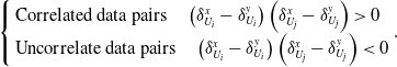 \begin{equation}\left\{ \begin{array}{l}{\textrm{Correlated data pairs}} \quad \left(\delta _{{U_i}}^x - \delta _{{U_i}}^y\right)\left(\delta _{{U_j}}^x - \delta _{{U_j}}^y\right) \gt 0\\{\textrm{Uncorrelate data pairs}}\quad \left(\delta _{{U_i}}^x - \delta _{{U_i}}^y\right)\left(\delta _{{U_j}}^x - \delta _{{U_j}}^y\right) \lt 0\end{array} \right.\! .\end{equation}
According to Equation (11), the Kendall correlation coefficient ${g_{i,j}}$
of
${g_{i,j}}$
of ${U_i}$
and
${U_i}$
and ${U_j}$
is calculated.
${U_j}$
is calculated.
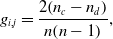 \begin{equation}{g_{i,j}} = \frac{{2\!\left( {{n_c} - {n_d}} \right)}}{{n\!\left( {n - 1} \right)}},\end{equation}
where ${n_c}$
and
${n_c}$
and ${n_d}$
are the number of correlated and uncorrelated data pairs, respectively.
${n_d}$
are the number of correlated and uncorrelated data pairs, respectively.
-
Overall Kendall correlation coefficient
${\eta _{{U_i}}}$
between nodes(12)
\begin{equation}{\eta _{{U_i}}} = \frac{{\sum\limits_{j = 1}^Z {{g_{i,j}}} }}{Z}.\end{equation}
-
Kendall coefficient weight
${\lambda _{{U_i}}}$
of each node(13)
\begin{equation}{\lambda _{{U_i}}} = \frac{{{\eta _{{U_i}}}}}{{\sum\limits_{i = 1}^Z {{\eta _{{U_i}}}} }}.\end{equation}
-
Integrating information entropy weight and Kendall coefficient weight, the weight of deviation transfer
${\rho _{{U_i}}}$
of each node is obtained(14)
\begin{equation}{\rho _{{U_i}}} = \frac{{\frac{{{e_{{U_i}}}}}{{{\lambda _{{U_i}}}}}}}{{\sum\limits_{i = 1}^Z {\frac{{{e_{{U_i}}}}}{{{\lambda _{{U_i}}}}}} }}.\end{equation}


In Equation (14), the weight ${\rho _{{U_i}}}$
represents the importance of nodes in deviation transfer.
${\rho _{{U_i}}}$
represents the importance of nodes in deviation transfer.
3.3 Construction of assembly deviation transfer function based on weighted transfer entropy
According to ${\rho _{{U_i}}}$
, the deviation transfer entropy is weighted, and the deviation transfer relationship between node
${\rho _{{U_i}}}$
, the deviation transfer entropy is weighted, and the deviation transfer relationship between node $U_{{L_\alpha }}^\mu $
and node
$U_{{L_\alpha }}^\mu $
and node $U_{{L_\beta }}^\nu $
is obtained.
$U_{{L_\beta }}^\nu $
is obtained.
 \begin{equation}{\delta _{U_{{L_\alpha }}^\mu \to U_{{L_\beta }}^\nu }} = {\rho _{U_{{L_\alpha }}^\mu }}{T_{U_{{L_\alpha }}^\mu \to U_{{L_\beta }}^\nu }}.\end{equation}
Extending Equation (15), the deviation transfer relationship between node $U_{{L_\beta }}^\nu $
and node
$U_{{L_\beta }}^\nu $
and node $U_{{L_\beta }}^\nu $
is obtained at the L
α
level.
$U_{{L_\beta }}^\nu $
is obtained at the L
α
level.
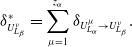 \begin{equation}\delta _{U_{{L_\beta }}^\nu }^ * = \sum\limits_{\mu {\rm{ = 1}}}^{{z_\alpha }} {{\delta _{U_{{L_\alpha }}^\mu \to U_{{L_\beta }}^\nu }}} .\end{equation}
Incorporating Equations (15) and (16), the deviation transfer contribution between node $U_{{L_\alpha }}^\mu $
and node
$U_{{L_\alpha }}^\mu $
and node $U_{{L_\beta }}^\nu $
is obtained.
$U_{{L_\beta }}^\nu $
is obtained.
 \begin{equation}\omega _{U_{{L_\alpha }}^\mu \to U_{{L_\beta }}^\nu }^{} = \frac{{\delta _{U_{{L_\alpha }}^\mu \to U_{{L_\beta }}^\nu }^{}}}{{\delta _{U_{{L_\beta }}^\nu }^ * }},\end{equation}
where the larger $\omega _{U_{{L_\alpha }}^\mu \to U_{{L_\beta }}^\nu }^{}$
is, the larger influence of the node
$\omega _{U_{{L_\alpha }}^\mu \to U_{{L_\beta }}^\nu }^{}$
is, the larger influence of the node $U_{{L_\alpha }}^\mu $
on the node
$U_{{L_\alpha }}^\mu $
on the node $U_{{L_\alpha }}^\mu $
is.
$U_{{L_\alpha }}^\mu $
is.
As shown in Fig. 2, the weighted deviation transfer entropy obtained by Equation (17) is used to describe relationships of transfer and accumulation between assembly deviations.

Figure 2. Assembly deviation transfer complex networks of complex thin-walled structures.

Figure 3. Key deviation source diagnosis of complex thin-walled structures.
4.0 The key deviation source diagnosis of complex thin-walled structures
4.1 The process of key deviation source diagnosis of complex thin-walled structures
The complex networks of deviation transfer have complex structures and many nodes. If it is directly used for assembly quality control without distinction, it will not be able to grasp the key factors. As shown in Fig. 3, the topological relationship of assembly structures is described by complex networks, and the causality of assembly deviation transfer is described by assembly feature transfer entropy. First, according to the assembly process information of complex thin-walled structures, assembly units are divided and the assembly sequences are defined. The assembly feature tree is constructed based on assembly units and assembly sequences. Then, assembly features are regarded as network nodes. The complex networks of assembly deviation transfer are constructed. Secondly, the information entropy theory of information theory is introduced to define the deviation transfer entropy. The assembly deviation transfer function based on transfer entropy is constructed to quantify the size and direction of deviation transfer between network nodes. Thirdly, the information entropy and Kendall coefficient are introduced to quantify the importance of network nodes objectively. The deviation transfer entropy is weighted according to the importance weight. Finally, the depth-first traversal algorithm is used to search deviation transfer paths. The size of the deviation transfer is quantified by transfer entropy. The degree centrality of complex networks is integrated to identify key deviation sources that affect the assembly quality of complex thin-walled structures.
4.2 Deviation transfer path search based on depth-first traversal algorithm
As shown in Fig. 4, the depth-first traversal algorithm is introduced to search the deviation transfer paths. First, the deviation source is recorded as the start point of deviation transfer paths. Second, taking the deviation source as the start point, the next assembly feature node that the deviation source can transmit to is explored, and the assembly feature node is recorded. Third, based on this assembly feature node, the algorithm will continue to explore and record the next assembly feature node that the deviation can transmit to until the next assembly feature node is not found. Moreover, the algorithm judges whether all assembly feature nodes are explored. If there exist unexplored assembly feature nodes, the algorithm returns to the superior to explore. Finally, if the algorithm returns to the deviation source, there still exist unrecorded assembly feature nodes. The algorithm will search other deviation sources until all assembly feature nodes are found and all deviation transfer paths are recorded.

Figure 4. Depth-first traversal algorithm to search deviation transfer path.
4.3 Key deviation source diagnosis based on degree centrality and global transfer entropy
4.3.1 Quantification of node importance
Degree centrality is an index for judging the importance of network nodes. The degree centrality is used to quantify the importance of nodes, which is calculated according to the number of edges in complex networks. Therefore, degree centrality is introduced to represent the importance ${C_{U_{{L_\alpha }}^\mu }}$
in deviation transfer networks.
${C_{U_{{L_\alpha }}^\mu }}$
in deviation transfer networks.
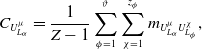 \begin{equation}{C_{U_{{L_\alpha }}^\mu }} = \frac{1}{{Z - 1}}\sum\limits_{\phi {\rm{ = 1}}}^\vartheta {\sum\limits_{\chi = 1}^{{z_\phi }} {{m_{U_{{L_\alpha }}^\mu U_{{L_\phi }}^\chi }}} } ,\end{equation}
where ${C_{U_{{L_\alpha }}^\mu }}$
denotes the degree centrality of node
${C_{U_{{L_\alpha }}^\mu }}$
denotes the degree centrality of node $U_{{L_\alpha }}^\mu $
.
$U_{{L_\alpha }}^\mu $
. $U_{{L_\phi }}^\chi $
denotes the
$U_{{L_\phi }}^\chi $
denotes the $\chi $
th network node in the
$\chi $
th network node in the ${L_\phi }$
level.
${L_\phi }$
level. ${z_\phi }$
denotes the total number of nodes in the
${z_\phi }$
denotes the total number of nodes in the ${L_\phi }$
level.
${L_\phi }$
level. $\vartheta $
denotes the total number of assembly levels.
$\vartheta $
denotes the total number of assembly levels.
 \begin{equation*}{m_{U_{{L_\alpha }}^\mu U_{{L_\phi }}^\chi }} = \left\{ {\begin{array}{*{20}{c}}1\\0\end{array}} \right.{\rm{ }}\begin{array}{*{20}{l}}{{\textrm{Deviation of node }}{\ }U_{{L_\alpha }}^\mu{\ }{\textrm{can}}{\ } {\textrm{be}}{\ } {\rm{passed}}{\ } {\textrm{to node }}{\ }U_{{L_\phi }}^\chi }\\{{\textrm{Deviation of node }}{\ }U_{{L_\alpha }}^\mu{\ } {\textrm{can not be}}{\ } {\textrm{passed}}{\ } {\textrm{to node }}{\ }U_{{L_\phi }}^\chi }\end{array}\!.\end{equation*}
4.3.2 Calculation of assembly deviation contribution
Incorporating Equations (17) and (18), key factors that affect the assembly accuracy of complex thin-walled structures are mined from two different perspectives, including network topology structures and deviation information transfer. The contribution $\psi $
of deviation sources for the assembly deviation of complex thin-walled structures is defined as
$\psi $
of deviation sources for the assembly deviation of complex thin-walled structures is defined as
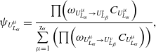 \begin{equation}{\psi _{U_{{L_\alpha }}^\mu }} = \frac{{\prod\! {\left( {{\omega _{U_{{L_\alpha }}^\mu \to U_{{L_\beta }}^\nu }}{C_{U_{{L_\alpha }}^\mu }}} \right)} }}{{\sum\limits_{\mu {\rm{ = 1}}}^{{{\rm{z}}_\alpha }} {\left( {\prod \!{\left( {{\omega _{U_{{L_\alpha }}^\mu \to U_{{L_\beta }}^\nu }}{C_{U_{{L_\alpha }}^\mu }}} \right)} } \right)} }},\end{equation}
where ${\psi _{U_{{L_\alpha }}^\mu }}$
is the contribution of deviation source
${\psi _{U_{{L_\alpha }}^\mu }}$
is the contribution of deviation source $U_{{L_\alpha }}^\mu $
for the assembly deviation of complex thin-walled structures.
$U_{{L_\alpha }}^\mu $
for the assembly deviation of complex thin-walled structures.
According to $\psi $
, the ranking is carried out. If the value of
$\psi $
, the ranking is carried out. If the value of $\psi $
is large, it represents that this deviation source has a great influence on the assembly deviation of complex thin-walled structures, namely this deviation source is more likely to be the key deviation source.
$\psi $
is large, it represents that this deviation source has a great influence on the assembly deviation of complex thin-walled structures, namely this deviation source is more likely to be the key deviation source.
5.0 Application
The central wing box is a typical complex thin-walled structure. As shown in Fig. 5, taking a certain type of aircraft central wing box as the object, the central wing box of the aircraft is riveted by many parts, including upper panel skin, upper panel stringer, lower panel skin, and lower panel stringer.
Table 1. Overall size of assembly units


Figure 5. Central wing box of an aircraft.
3DCS software is a typical simulation software of aircraft assembly tolerance. It can be used to calculate the assembly deviations of rigid-flexible coupling parts. First, 3DCS software is used to simulate the assembly deviation of the central wing box to obtain deviation data of assembly features. Second, based on the assembly feature deviation data, complex network theory, and transfer entropy theory are used to calculate the assembly deviation transfer. Finally, by comparing the calculation results of assembly deviation transfer and direct simulation results of 3DCS software, the correctness, and feasibility of the assembly deviation transfer and key deviation source diagnosis method are verified for complex thin-walled structures. The overall sizes of the central wing box are shown in Table 1, and the material of assembly parts is aluminum-lithium alloy. As shown in Fig. 6, assembly levels are divided and the assembly sequences are clarified, according to the assembly process of the central wing box.
5.1 Assembly feature definition
According to the assembly process information of the central wing box, assembly features are defined as shown in Tables 2, 3 and 4. The meaning of position degree is position deviation of the axis of the hole relative to the central axis.
Table 2. Assembly features of the first level

Table 3. Assembly features of the second level
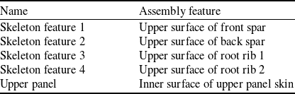
Table 4. Assembly features of the third level


Figure 6. Assembly level division of central wing box.
5.2 Assembly deviation transfer network node definition
According to assembly levels, assembly sequences shown in Fig. 6, and assembly characteristics shown in Table 2, 3 and 4, assembly deviation transfer network nodes of the central wing box are defined as shown in Table 5.
Table 5. Assembly deviation transfer network nodes of the central wing box

3DCS software is used to simulate 12 times. Assembly deviation transfer data are obtained as shown in Tables 6, 7 and 8. The values in Table 6 are input data, and the values in Table 7 and 8 are output data.
Table 6. Assembly feature deviation of the first level (mm)

Table 7. Assembly feature deviation of the second level (mm)

5.3 Assembly deviation transfer
5.3.1 Assembly deviation transfer based on complex networks and weighted transfer entropy
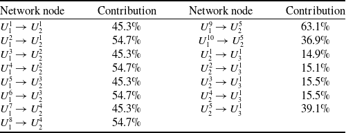
Using Equations (1)–(5), the transfer entropy between network nodes is calculated based on assembly feature deviation data in Tables 6, 7 and 8. Using Equations (6)–(13), the importance weights of nodes are calculated as shown in Table 10. According to Tables 9 and 10, quantitative relationships of deviation transfer between network nodes are calculated by Equation (14), as shown in Table 11. Incorporating Equations (15) and (16), deviation transfer contributions between network nodes are calculated as shown in Table 12, according to Table 11.
Table 8. Assembly feature deviation of the third level (mm)

Table 9. Transfer entropy between network nodes

Table 10. Importance weight of nodes
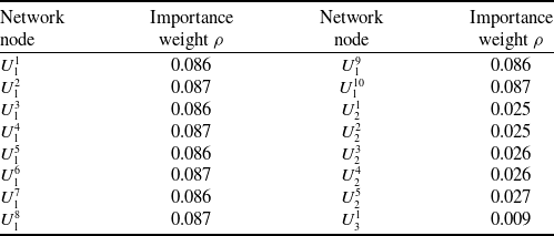
Table 11. Deviation transfer relationship between network nodes

Table 12. Deviation transfer contributions between network nodes based on complex network and weighted transfer entropy
5.3.2 Assembly deviation sensitivity simulation based on 3DCS
3DCS is used to carry out the assembly deviation sensitivity simulation. Deviation transfer contributions between network nodes are shown in Table 13.
Table 13. Deviation transfer between network nodes based on 3DCS
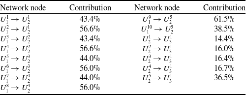
By comparing Tables 12 and 13, deviation transfer contributions calculated by the two methods are almost the same. The deviation range of contributions is from 0.9% to 2.6%. It verifies the correctness of the deviation transfer method based on complex networks and weighted transfer entropy. The reasons for some differences in contributions are as follows. When analysing the deviation transfer, the 3DCS simulation software regards the importance of each network node as the same. Information entropy and Kendall coefficient are used to quantify the importance of deviation transfer nodes by the deviation transfer analysis method proposed in this paper. According to this, the deviation transfer entropy is weighted.
The sensitivity analysis method diagnoses the key deviation source exclusively dependent on the deviation data and does not consider the assembly relationship between the assembly components. When the variation propagation method is applied to diagnose the key deviation source, the variation propagation modeling process of flexible parts is very complex and the quantity of computation is large. Compared with the sensitivity analysis method and variation propagation method, the key deviation source diagnosis method proposed in this paper diagnoses the key deviation source from the two perspectives of structural topology and deviation information transmission. This method uses the complex network to describe the assembly relationship of each part and uses the weighted transfer entropy to quantify the deviation transfer quantity. Therefore, the method proposed in this paper can more effectively diagnose the key deviation source of aircraft structures.
5.4 Key deviation source diagnosis
5.4.1 Key deviation source diagnosis based on degree centrality and global transfer entropy
Based on Table 5, the depth-first traversal algorithm is used to search deviation transfer paths. Setting the node $U_1^{\rm{1}}$
as the start point, the deviation transfer of the central wing box is searched to obtain deviation transfer paths as shown in Table 14. Based on Table 14, the degree centrality of network nodes is calculated as shown in Table 15, according to Equation (17). Using Equation (18), contributions of each deviation source to the assembly deviation of the central wing box are obtained by calculation as shown in Table 16, according to Tables 14 and 15.
$U_1^{\rm{1}}$
as the start point, the deviation transfer of the central wing box is searched to obtain deviation transfer paths as shown in Table 14. Based on Table 14, the degree centrality of network nodes is calculated as shown in Table 15, according to Equation (17). Using Equation (18), contributions of each deviation source to the assembly deviation of the central wing box are obtained by calculation as shown in Table 16, according to Tables 14 and 15.
Table 14. Deviation transfer path
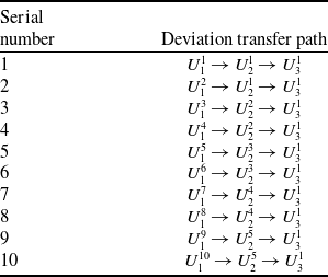
Table 15. Degree centrality of network nodes

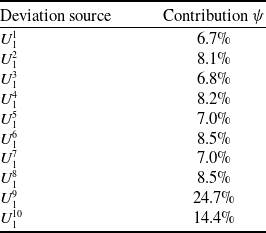
Table 16. Contribution of deviation source to assembly deviation
5.4.2 Key deviation source diagnosis based on 3DCS
3DCS is used to simulate the contributions of deviation sources directly. Contributions of assembly deviations are shown in Table 17.
Table 17. Key deviation source simulation based on 3DCS

By comparing Tables 16 and 17, some conclusions can be drawn as follows.
-
(1) The contribution size of each deviation source to product assembly deviation can be obtained by two methods, and the difference of contributions is within 3%.
-
(2) Key deviation sources that affect assembly quality can be diagnosed by two methods. The key deviation source is the position deviation of the upper panel skin positioning hole.
-
(3) There are some differences between the two methods of contributions ranking, such as deviation sources
$U_{\rm{1}}^{\rm{3}}$
and
$U_{\rm{1}}^{\rm{5}}$
, because the equability weight method is utilised to analyse deviation transfer. However, the weights are assigned to deviation transfer contributions by the diagnosis method proposed in this paper, based on the degree centrality algorithm and global transfer entropy. It can make diagnosis results closer to the actual operation. Therefore, the diagnosis method proposed in this paper can more objectively realise the key deviation source diagnosis.


6.0 Conclusion
Aimed at the assembly of complex thin-walled structures such as aircraft, the deviation transfer between deviation sources and structural parts has the characteristics of small sample size, nonlinearity and strong coupling. This paper proposes a key deviation sources diagnosis method for complex thin-walled structure deviations based on weighted transfer entropy and complex networks. This method analyses key deviation sources from two different aspects including network topology structures and deviation information transfer. Transfer relationships of assembly feature deviations are quantified to accurately diagnose key deviations that affect assembly quality.
The application shows that all key deviation sources can be diagnosed by 3DCS software simulation and the key deviation diagnosis method proposed in this paper. And the difference of each deviation source contribution is within 3 %, so the correctness is verified. There exists some diversity between the two methods of contribution ranking because differences in node importance are not able to be considered by 3DCS software. The weights are assigned to contributions by the diagnosis method proposed in this paper. It makes diagnostic results more accurate and reliable.
This method is not only suitable for the transfer and analysis of aircraft assembly deviations but also suitable for products of complex thin-walled structures such as aerospace. It has important theoretical significance and practical engineering value for optimising assembly tolerance design, reducing development costs and improving assembly quality.
Acknowledgements
The authors would like to thank the National Natural Science Foundation of China [51865037] and Aeronautical Science Foundation of China [2019ZE056004] for their financial support.
Author contribution
Yongguo Zhu: methodology, data collection and analysis, writing–review and editing. Qiang Shi: data collection and analysis, writing–original draft. Weipeng Jiang: data curation, validation, supervision. Bin Deng: investigation, writing–review and editing.
Funding
Supported by National Natural Science Foundation of China [51865037] and Aeronautical Science Foundation of China [2019ZE056004].
Ethics approval
The authors declare that this manuscript was not submitted to more than one journal for simultaneous consideration. Also, the submitted work is original and not has been published elsewhere in any form or language.
Consent to participate and publish
The authors declare that they participated in this paper willingly and the authors declare to consent to the publication of this paper.
Competing interests
No potential competing interest was reported by the author(s).


