


Nomenclature
- ANSP
-
air navigation service provider
- ATM
-
air traffic management
- CDA
-
continuous descent approach
- CPS
-
constrained position shifting
- DP
-
dynamic programming
- EP
-
entry point
- FAF
-
final approach fix
- FAP
-
final approach path
- FCFS
-
first come first served
- FDP
-
final approach descent point
- LTFJ
-
Istanbul Sabiha Gökçen Airport
- MILP
-
mixed-integer linear programming
- MINLP
-
mixed-integer nonlinear programming
- MIP
-
mixed-integer programming
- PMS
-
Point Merge System
- REP
-
runway entry point
- RHC
-
rolling horizon control
- TMA
-
terminal manoeuvring area
- TFA
-
top of final approach point
- TOD
-
top of descent
- TW
-
time window
- VM
-
vector manoeuvre
1. Introduction
1.1 Motivation
TMA is a key component of an airport’s operations, as it is responsible for managing the flow of arriving and departing aircraft within a certain radius of the airport. The efficiency of the TMA has a direct impact on the overall capacity of the airport, as it determines how quickly and smoothly aircraft can be sequenced for arrival and departure. Some of the factors that can influence the relationship between TMA traffic flow and airport capacity are flight schedules, runway design and configuration in use, airspace design, traffic mix of aircraft categories traffic distribution of arrival and departure operations, air traffic control (ATC) facilities and equipment, the performance of air traffic controllers and pilots, predominant weather conditions and environmental constraints [Reference Janic1].
The annual global air traffic growth was 3.5% on average between 1990 and 2019 [2]. Although the COVID-19 pandemic led to a 48% decrease in total passenger flights in 2020 compared to the previous year [3], air travel demand is almost recovered to 2019 values by 2023 [4]. Despite the temporary decline in demand, the air transportation industry has proven its resilience in growth against global economic, social, and political crises since the 1950s [Reference Oxley and Jain5]. Therefore, the previously projected traffic volumes can still be met in long term until the 2040s as forecasted by ICAO [6]. This anticipated growth will increase airborne and ground delay resulting in congestion and additional fuel in TMAs around the major airports. The improvement of airport operations, therefore, has been determined as one of the key research areas both in ICAO’s Global Air Navigation Plan and SESAR’s vision towards the 2050s [7,8]. In this regard, the careful planning of arriving and departing traffic flows within the TMAs is imperative to ensure a seamless and globally coordinated provision of air navigation services and to implement performance-based operations across the entire air traffic management (ATM) network. Decision support and/or automation systems based on mathematical programming algorithms can be very effective tools to achieve a more accurate and efficient way to plan and coordinate the movement of aircraft within the TMA. These algorithms can help to optimise the sequencing and scheduling of aircraft within the TMA by considering all relevant constraints and objectives, including separation requirements, aircraft performance and airspace constraints. Especially the inclusion of more realistic aircraft performance models can further improve the accuracy of the solutions to be implemented by air traffic controllers.
The primary goal of this study was to develop a more realistic sequencing model with a multi-objective approach that minimises the total delay and total fuel in mixed operations. The model involves both arrival and departure operations and adopts the concerns of different stakeholders such as airlines and air navigation service providers (ANSPs). In this study, the $\varepsilon$
-constraint method was preferred because it allows all non-dominated points located in both non-convex and convex parts of the image set to be obtained. Therefore, the approach of the proposed solution will be capable of supporting the current and developing automation of decision-support systems for enhanced airport operations.
$\varepsilon$
-constraint method was preferred because it allows all non-dominated points located in both non-convex and convex parts of the image set to be obtained. Therefore, the approach of the proposed solution will be capable of supporting the current and developing automation of decision-support systems for enhanced airport operations.
1.2 Literature review
Numerous studies have been performed on the arrival/departure sequencing and scheduling problem for efficient runway management. Some studies have focused only on the optimisation of arrival sequencing using mixed-integer linear programming (MILP) along with heuristic algorithms [Reference Beasley, Krishnamoorthy, Sharaiha and Abramson9], receding horizon control (RHC) [Reference Hu and Chen10], dynamic programming (DP) [Reference Lieder, Briskorn and Stolletz11] and letter sequencing algorithms [Reference Kwasiborska12]. Hu and Paolo studied the benefits of using the neighbouring relationship between aircraft pairs to construct chromosomes for genetic algorithms [Reference Hu and Di Paolo13]. Lee and Balakrishnan developed a DP algorithm including a constrained position shifting (CPS) approach on a single runway [Reference Lee and Balakrishnan14]. Vadlamani and Hosseini [Reference Vadlamani and Hosseini15] introduced an adaptive large neighbourhood search algorithm for the same problem. Briskorn and Stolletz [Reference Briskorn and Stolletz16] proposed a MILP model for arrivals on multiple runways. All of these studies treated the problems as a single-objective optimisation problem and attempted to minimise a total cost function formulated as a linear function of deviation from targeted arrival time, makespan and airborne delay as a result of position shifting or holding. Zuniga et al. [Reference Zuniga, Delahaye and Piera17] extended the sequencing problem for arrivals along multiple merging routes within the TMAs. Kaplan and Çetek [Reference Kaplan and Çetek18] proposed the Clonal Selection Algorithm (CSA) to solve the arrival sequencing problem with a CPS approach. Çeçen and Aybek Çetek [Reference Cecen and Aybek Çetek19] presented a two-step MILP model to minimise total conflict resolution time and total airborne delay using lexicographic goal programming. Ikli et al. [Reference Ikli, Mancel, Mongeau, Olive and Rachelson20] presented a focused review of the most relevant techniques in the recent literature on the runway scheduling problem. Gui et al. [Reference Gui, Le, Huang, Zhang and D’Ariano21] proposed a scheduling model and generated conflict-free trajectories using a lateral path stretching method.
Balakrishnan and Chandran, Rathinam et al., and Gupta et al. [Reference Balakrishnan and Chandran22–Reference Gupta, Malik and Jung24] dealt with departure sequencing problem using DP and MILP techniques. These approaches attempted to find the optimal solutions for single-objective functions, including runway throughput and delay.
Various researchers have proposed models for the solution of combined arrival and departure sequencing problems using various approaches, such as greedy algorithms along with simulated annealing and Meta-RaPS metaheuristics [Reference Hancerliogullari, Rabadi, Al-Salem and Kharbeche25], MILP with optimisation-based heuristics [Reference Farhadi, Ghoniem and Al-Salem26], stochastic branch-and-bound algorithm [Reference Sölveling and Clarke27] and simulated annealing [Reference Rodríguez-Díaz, Adenso-Díaz and González-Torre28]. These combined approaches have been formulated as single-objective function optimisation problems minimising the total weighted delay, total fuel cost (as a linear function of time) and makespan. Sölveling et al. [Reference Solveling, Solak, Clarke and Johnson29] developed a two-stage stochastic algorithm that took the time spent on pushback and taxiway into account for runway scheduling in the presence of uncertainty. Al-Salem et al. [Reference Al-Salem, Farhadi, Kharbeche and Ghoniem30] proposed a mixed-integer programming (MIP) model with the objective function of minimising the total weighted tardiness of operations over multiple runways. Heidt et al. and Rocha Murça and Müller [Reference Heidt, Helmke, Liers and Martin31,Reference Murça and Müller32] used the DP method and presented MINLP and MILP models, respectively, to minimise the total delay cost. Ng et al. [Reference Ng, Lee, Chan and Qin33] dealt with mixed-mode parallel operations to investigate the potential of using the min-max regret approach under the uncertainty of delays.
Several studies have presented optimal solution approaches to the arrival-departure sequencing problem on route networks within the TMAs. Gilbo [Reference Gilbo34] considered arrival and departure as two interdependent processes with fixes to minimise the delay. Balakrishnan and Chandran [Reference Balakrishnan and Chandran35] presented DP algorithms with CPS to seek several objective functions separately, such as makespan, maximum delay and total delay. Samà et al. [Reference Samà, D’Ariano and Pacciarelli36] compared the first-come-first-served (FCFS) and branch-and-bound algorithm solutions in terms of delays. They used the RHC for dynamically scheduling aircraft. In subsequent study, they presented a MIP model for aircraft scheduling and routing, assuming fixed routing and used a combined branch-and-bound, and tabu search optimisation-based approach [Reference Samà, D’Ariano, D’Ariano and Pacciarelli37]. Desai and Prakash [Reference Desai and Prakash38] studied mixed-mode operations on a single runway along with a TMA model and developed a MILP formulation to minimise total delay. Lieder and Stolletz [Reference Lieder and Stolletz39] examined interdependent runway operations within the extended TMA to minimise total delay cost using DP. Samà et al. (Reference Samà, D’Ariano, Palagachev and Gerdts40) proposed the MILP model for the scheduling problem to minimise delays, travel times and fuel. Çecen [Reference Cecen41] aimed to minimise fuel in extended TMA using the MILP model.
There are some studies in the literature that adopted the multi-objective nature of the problem. Tang et al. [Reference Tang, Wang, Cao and Zhang42] dealt with arrival scheduling using a multi-objective neighbourhood search technique to minimise total cost and scheduled time. Zhang et al. [Reference Zhang, Zhao, Zhang, Dai and Sui43] proposed a criteria selection method and presented a multi-objective model for arrivals. They elaborated on different criteria for this problem, namely, maximum completion time, flow time, tardiness time, total completion time and flow time. Montoya et al. [Reference Montoya, Rathinam and Wood44] used DP to minimise total delay and departure makespan. Bennell et al. [Reference Bennell, Mesgarpour and Potts45] developed a multi-objective formulation for the arrival sequencing problem with several objective functions, such as runway throughput, earliness and lateness, additional flight time and fuel cost. Hong et al. [Reference Hong, Cho, Kim and Choi46] proposed a multi-objective formulation for Point Merge System (PMS) including the CPS framework. While the studies by Montoya et al. and Bennell et al. used the weighted sum method to bring together individual objectives, the research by Hong et al. used the $\varepsilon$
-constraint method where objectives were total flight time and the number of sequence changes. Liang et al. [Reference Liang, Delahaye and Maréchal47] proposed Multi-Level PMS for arrivals to minimise the total number of conflicts, average square delay and makespan objectives. They implemented the RHC to reduce computational burden and uncertainty. Liang et al. [Reference Liang, Delahaye and Marechal48] improved the Multi-Level PMS route network for both arrivals and departures and included average operation interval and total position shifting as objective functions in addition to those in their earlier study. However, both studies converted the multi-objectives to single-objective using the linear scalarisation method. Çeçen [Reference Cecen49] proposed a MILP model using PMS with two objective functions, which are minimising total delay and the total number of conflict resolution manoeuvres. Dönmez et al. [Reference Dönmez, Çetek and Kaya50] considered taxi-in and taxi-out times of operations while implementing the parallel PMS in TMA. Later, they proposed a stochastic model and compared deterministic and stochastic solutions with the FCFS approach under wind uncertainties [Reference Dönmez, Çetek and Kaya51]. Yin et al. [Reference Yin, Ma, Hu, Han, Yin and Xie52] investigated trade-offs between the delay, throughput, and emission on the runway in the presence of uncertainty.
$\varepsilon$
-constraint method where objectives were total flight time and the number of sequence changes. Liang et al. [Reference Liang, Delahaye and Maréchal47] proposed Multi-Level PMS for arrivals to minimise the total number of conflicts, average square delay and makespan objectives. They implemented the RHC to reduce computational burden and uncertainty. Liang et al. [Reference Liang, Delahaye and Marechal48] improved the Multi-Level PMS route network for both arrivals and departures and included average operation interval and total position shifting as objective functions in addition to those in their earlier study. However, both studies converted the multi-objectives to single-objective using the linear scalarisation method. Çeçen [Reference Cecen49] proposed a MILP model using PMS with two objective functions, which are minimising total delay and the total number of conflict resolution manoeuvres. Dönmez et al. [Reference Dönmez, Çetek and Kaya50] considered taxi-in and taxi-out times of operations while implementing the parallel PMS in TMA. Later, they proposed a stochastic model and compared deterministic and stochastic solutions with the FCFS approach under wind uncertainties [Reference Dönmez, Çetek and Kaya51]. Yin et al. [Reference Yin, Ma, Hu, Han, Yin and Xie52] investigated trade-offs between the delay, throughput, and emission on the runway in the presence of uncertainty.
There are different stakeholders in the air transportation system, including ANSPs, airlines, airports and aviation authorities. Each of them has its own set of objectives. For example, ANSP aims to ensure the safety and efficiency of the aircraft. Airlines want to minimise fuel costs, maximise the punctuality of flights and achieve fairness between airlines. Airports have the goal of maximising throughput. Aviation authorities look to minimise environmental effects, such as noise and emissions. Among these objectives, our research aims to minimise total fuel and delay in mixed operations, as these are especially critical performance indicators for both airlines and ANSPs. To minimise these two objectives, we formulated a mathematical model that considers the nonlinear dependencies on aircraft performance parameters, such as airspeed, bank angle and altitude, and uses vector manoeuvre (VM) to achieve assigned operational times. Most of the studies considering aircraft scheduling problem as multi-objective converted individual objectives to single-objective function using the weighted sum method. There are two major drawbacks to this approach. First, the weighted-sum method ensures Pareto optimal solutions for linear models only. Second, to achieve an accurate representation of the real-world problem, user-supplied weights should be selected with great care to achieve the right solution in the Pareto optimal front [Reference Ehrgott53].
An effective arrival-departure sequencing model which can be implemented into real-world ATM systems should successfully deal with these issues to support enhanced airport operations in terms of efficient capacity use and traffic flow management.
1.3 Contribution of the research
The main contributions of this study are listed as follows:
-
(1) An improved multi-objective formula is presented to reflect the trade-off between total delay and total fuel, which are two critical and conflicting performance indicators of the airlines and ANSPs. The previous studies described fuel as a linear function of time. Therefore, they did not consider them as conflicting objectives. Thus, realistic features of flight operations within the TMAs were not accurately included in objective functions and constraints.
-
(2) The proposed mathematical model considers realistic VM to achieve assigned operational times. While formulating these manoeuvres, nonlinear dependencies on airspeed, bank angle and altitude were considered based on realistic aerodynamics and propulsive characteristics of aircraft. Therefore, both objective functions can be calculated more accurately. Despite this complex nonlinear representation, the proposed model can generate non-dominated solutions in less than 5min for high traffic densities.
-
(3) The model generates optimal trajectories using VM, minimising both objective functions simultaneously. Therefore, both conflict resolution and aircraft sequencing and scheduling tasks can be done in a single step rather than in two steps as in Cecen and Cetek [Reference Cecen and Cetek54].
1.4 Organisation of paper
The remaining parts of the paper are organised as follows. The problem, airspace structure, and traffic flow are defined in Section 2 where we also introduce VM and fly-by-turn to the final approach path (FAP). We also present the fuel flow model in this section. Section 3 presents the proposed model for the defined problem. We give inputs and parameters for the implementation of the proposed model in Section 4. Computational experiments are also reported in this section. Finally, the concluding remarks are documented in Section 5.
2.0 Problem statement
2.1 Airspace and traffic flow
Controlled airspace, a volume of earth’s atmosphere of defined geometry and size, accommodates flights with relevant ATC services according to its type (i.e. en-route sectors, airport control zones, and TMAs). TMAs are controlled airspaces founded at the confluence of air traffic service routes in the neighbourhood of one or more airports [55]. The monitoring, sequencing and separation management of flights within the TMAs are usually more complex than those of other airspaces because they contain a complex network of converging or intersecting routes around airports. Air traffic controllers should conventionally use vectoring techniques consisting of necessary heading, speed and altitude change instructions to aircraft to maintain safe and efficient air traffic flow. On the other hand, it is more difficult to provide an efficient traffic flow while ensuring the safe separation between aircraft especially at peak traffic hours when the airports have maximum demand. Air traffic controllers often implement higher time and distance separations than the necessary minima by delaying aircraft in the air or on the ground. These delays lead to decreased utilisation of runways and inefficient sequencing with extra flight times, distances and fuel. In this study, we focus on obtaining efficient sequences with minimum delay and fuel within the TMA during hours with high traffic demand.
In order to approach this problem, we adopted a generic TMA surrounding an airport with a single runway (Fig. 1). The runway serves for arrivals and departures. Arrivals are supposed to enter the TMA from a set of predefined entry points (EPs). Each arrival entering TMA from its associated EP at a known entry time, speed and altitude should follow a conflict-free trajectory to the merge point, called the final approach fix (FAF), using a vectoring manoeuvre.

Figure 1. A generic TMA configuration (top view).
As soon as the aircraft has arrived at its EP, it is directed to fly to FAF along the described descent profile in Fig. 2. The aircraft is required to perform level flight at its initial flight altitude and speed until it reaches the top of descent (TOD) point and then it commences continuous descent approach (CDA) until it arrives to the predefined final approach descent point (FDP). The CDA time and distance between TOD and FDP depend on the category and initial flight level of the aircraft. As the aircraft descends to FDP, it performs level flight and then fly-by-turn at FAF with a constant speed to align with FAP. As soon as the aircraft establishes the FAP, it performs level flight at FAF altitude and speed until it reaches the top of final approach point (TFA). This point depends on the aircraft category. Finally, the aircraft approaches along this common path and lands on the runway at the runway entry point (REP).

Figure 2. The descent profile of arrival within the TMA (side view).
Departures should wait for their take-off in the departure queue (DQ) at a designated area called the “holding point” located at the runway holding position. Here, they line up in the sequence determined by air traffic controllers and proceed towards the runway. The duration of waiting time at the holding point may vary depending on the density and traffic of the runway. Departure aircraft begin their take-offs from REP at their assigned operation time. If there is no delay requirement due to the wake turbulence separation, the departures enter the runway and take off. It is assumed that consecutive departures follow different flight paths rather than a common departure path therefore no crossing or overtaking conflicts occur between them within the TMA. It is also assumed that all arrival and departure routes are separated vertically to forbid crossing conflicts between them within the TMA. By these two assumptions, the safe separation is ensured between departure and departure or departure and arrival operations and no additional delay is required for the departures after take-off. Therefore, the flight time of departures within the TMA is not considered in the study, as it will not be affected by conflicts between any departure aircraft and others.
Estimated operation times of arrival and departure aircraft are known in advance. The operation times and sequences of each aircraft are determined based on these estimated times. Thus, estimated REP times of arrivals and departures, TMA entry point and altitude of arrivals, and aircraft performance category are the input parameters of the model. The output of the model consists of assigned operation times and sequences, total delay, total fuel consumption, VM variables to absorb the delay and fly-by-turn variables to align with the FAP. Additionally, the model calculates the CDA start time at the TOD point, fly-by-turn start and end time, and the start time of descent on the FAP to obtain the flight trajectory and profile of an arrival aircraft with necessary variables.
2.2 Separations
When the separation at the closest point between any aircraft pair is less than the specified safety minimum, a collision risk arises between them, which is referred to as conflict. Therefore, safe separation should be ensured for all aircraft within the TMA including runways, FAP and arrival/departure routes based on the required minima. Time separation minima between consecutive operation pairs on the runway and/or FAP are presented in Table 1 according to aircraft categories [Reference Balakrishnan and Chandran35]. These categories are set according to the maximum take-off mass of aircraft as heavy(H) (≥116,000kg), large(L) (19,000–116,000kg) and small(S) (≤19,000kg) [Reference De Neufville and Odoni56].
Table 1. Separation requirements (s) [Reference Balakrishnan and Chandran35]

Besides the wake turbulence separation minima on FAP and runway, aircraft should be separated on arrival and departure routes using minimum radar separation distance $(sep_{ij}^{radar})$
. This distance is specified as 3 nautical miles (nm) within the TMAs in the regulations. Two types of conflict can emerge between consecutive aircraft on arrival routes: (a) trailing conflict along the same route and (b) crossing conflict for converging routes (Fig. 3). The interarrival times between leading aircraft i and trailing aircraft j should be estimated at TOD, FDP and FAF points using aircraft speeds, entry times and distances at each route segment. At each point, the interarrival times should be greater or equal to the minimum radar separation time
$(sep_{ij}^{radar})$
. This distance is specified as 3 nautical miles (nm) within the TMAs in the regulations. Two types of conflict can emerge between consecutive aircraft on arrival routes: (a) trailing conflict along the same route and (b) crossing conflict for converging routes (Fig. 3). The interarrival times between leading aircraft i and trailing aircraft j should be estimated at TOD, FDP and FAF points using aircraft speeds, entry times and distances at each route segment. At each point, the interarrival times should be greater or equal to the minimum radar separation time $(t_{ij}^{radar})$
so that
$(t_{ij}^{radar})$
so that $sep_{ij}^{radar}$
is not violated at any moment along same arrival routes. In case the trailing aircraft is faster than the leading aircraft, no overtaking is allowed but the trailing aircraft is delayed to ensure the required minimum separation.
$sep_{ij}^{radar}$
is not violated at any moment along same arrival routes. In case the trailing aircraft is faster than the leading aircraft, no overtaking is allowed but the trailing aircraft is delayed to ensure the required minimum separation.

Figure 3. Conflict geometries: (a) same route, (b) converging routes (top view).
Besides the trailing conflicts along the routes, the crossing conflicts are checked at FAF for each consecutive aircraft from different arrival routes. In this case, the value of $t_{ij}^{radar}$
depends not only on relative airspeeds
$t_{ij}^{radar}$
depends not only on relative airspeeds $(\nu _i^{\,faf},\;\nu _j^{\,faf})$
of the aircraft pair and
$(\nu _i^{\,faf},\;\nu _j^{\,faf})$
of the aircraft pair and $sep_{ij}^{radar}$
but also the conflict geometry of routes intersecting with the angle
$sep_{ij}^{radar}$
but also the conflict geometry of routes intersecting with the angle ${\theta _{ij}}$
as shown in Fig. 3(b). Equation (1) estimates
${\theta _{ij}}$
as shown in Fig. 3(b). Equation (1) estimates $t_{ij}^{radar}$
for two aircraft flying at constant speed along intersecting linear trajectories [Reference Vela, Solak, Singhose and Clarke57]:
$t_{ij}^{radar}$
for two aircraft flying at constant speed along intersecting linear trajectories [Reference Vela, Solak, Singhose and Clarke57]:
 \begin{align}t_{ij}^{radar} = \frac{{sep_{ij}^{radar}}}{{\nu _i^{\,faf}\nu _j^{\,faf}\left| {\sin {\theta _{ij}}} \right|}}\sqrt {{{\left( {\nu _i^{\,faf}} \right)}^2} + {{\left( {\nu _j^{\,faf}} \right)}^2} - 2\nu _i^{\,faf}\nu _j^{\,faf}\cos {\theta _{ij}}} \;\;.\end{align}
2.3 VM and fly-by-turn to FAP
In order to ensure safe separation between operations, delayed aircraft are allowed to perform VMs in the horizontal plane at the EP level. The velocity of the aircraft $(\nu _i^{ep})$
is not changed during the VM. The VM is represented as vector deflection consisting of coordinated turns and level flight sections, as shown in Fig. 4 [Reference Cecen and Cetek54]. The deflection angle
$(\nu _i^{ep})$
is not changed during the VM. The VM is represented as vector deflection consisting of coordinated turns and level flight sections, as shown in Fig. 4 [Reference Cecen and Cetek54]. The deflection angle $\left(\psi _i^{vm}\right)$
from the original flight route, bank angle
$\left(\psi _i^{vm}\right)$
from the original flight route, bank angle $\left(\phi _i^{vm}\right)$
, and manoeuver distance
$\left(\phi _i^{vm}\right)$
, and manoeuver distance $\left(l_i^{vm}\right)$
are decision variables adjusted by the mathematical model to achieve required delay. The turning radius
$\left(l_i^{vm}\right)$
are decision variables adjusted by the mathematical model to achieve required delay. The turning radius $\left(r_i^{vm}\right)$
, distance traveled along the arc
$\left(r_i^{vm}\right)$
, distance traveled along the arc $\left(a_i^{vm}\right)$
, projected arc distance on the original flight route
$\left(a_i^{vm}\right)$
, projected arc distance on the original flight route $\left(b_i^{vm}\right)$
and level flight distance
$\left(b_i^{vm}\right)$
and level flight distance $\left(h_i^{vm}\right)$
are the other variables that are calculated based on angle and manoeuver distance variables.
$\left(h_i^{vm}\right)$
are the other variables that are calculated based on angle and manoeuver distance variables.

Figure 4. VM (top view).
Aircraft perform a fly-by-turn consisting of only coordinated turn with constant speed to align with FAP (Fig. 5). The relative bearing $\left(\psi _i^{\,fb}\right)$
between the original flight route and FAP is constant, but it varies for different arrival routes. The fly-by-turn is performed at FAF altitude. Therefore, the velocity of the aircraft
$\left(\psi _i^{\,fb}\right)$
between the original flight route and FAP is constant, but it varies for different arrival routes. The fly-by-turn is performed at FAF altitude. Therefore, the velocity of the aircraft $\left(\nu _i^{\,fb}\right)$
during the turning does not change. The turning radius
$\left(\nu _i^{\,fb}\right)$
during the turning does not change. The turning radius $\left(r_i^{\,fb}\right)$
, distance traveled along the arc
$\left(r_i^{\,fb}\right)$
, distance traveled along the arc $\left(a_i^{\,fb}\right)$
, and fly-by-turn distance
$\left(a_i^{\,fb}\right)$
, and fly-by-turn distance $\left(l_i^{\,fb}\right)$
performed on the arrival route and FAP are calculated based on bank angle decision variable
$\left(l_i^{\,fb}\right)$
performed on the arrival route and FAP are calculated based on bank angle decision variable $\left(\phi _i^{\,fb}\right)$
.
$\left(\phi _i^{\,fb}\right)$
.

Figure 5. Fly-by-turn to FAP (top view).
2.4 Fuel flow model
The Eurocontrol Base of Aircraft Data (BADA) performance model, providing the performance parameters for each aircraft type, was used to calculate the total fuel of aircraft during level flight, descent, VM and fly-by-turn. It was also used to estimate the required horizontal distance and time during CDA for given start and end flight levels [58].
2.4.1 Arrival fuel flow
The fuel flow rates per unit distance during level flight and descent for arrivals can be estimated using BADA performance parameters, such as aircraft mass (W), wing surface area (S), parasitic drag coefficient $({C_{D0}})$
, induced drag coefficient (dc), thrust specific fuel coefficients
$({C_{D0}})$
, induced drag coefficient (dc), thrust specific fuel coefficients $({C_{f1}}$
and
$({C_{f1}}$
and ${C_{f2}})$
, descent fuel flow coefficients
${C_{f2}})$
, descent fuel flow coefficients $({C_{f3}}$
and
$({C_{f3}}$
and ${C_{f4}})$
and cruise fuel flow correction coefficient
${C_{f4}})$
and cruise fuel flow correction coefficient $({C_{fcr}})$
. It is assumed that the airspeed of any aircraft does not change during level flight, and all aircraft perform CDA in the TMA [58].
$({C_{fcr}})$
. It is assumed that the airspeed of any aircraft does not change during level flight, and all aircraft perform CDA in the TMA [58].
In order to estimate fuel consumption, lift coefficient $({C_L})$
, drag coefficient
$({C_L})$
, drag coefficient $({C_D})$
and aerodynamic drag force (Drag) acting on aircraft at any altitude (alt) with density
$({C_D})$
and aerodynamic drag force (Drag) acting on aircraft at any altitude (alt) with density $(\rho )$
should be calculated as given in Equations (2), (3) and (4), respectively. It is assumed that the true airspeed
$(\rho )$
should be calculated as given in Equations (2), (3) and (4), respectively. It is assumed that the true airspeed $(\nu )$
of any aircraft does not change during level flight. However, the value of
$(\nu )$
of any aircraft does not change during level flight. However, the value of $\nu $
changes with altitude. In level flight, the bank angle
$\nu $
changes with altitude. In level flight, the bank angle $(\phi )$
is equal to zero.
$(\phi )$
is equal to zero.
 \begin{align}{C_L} = \frac{{2W/S}}{{\rho {\nu ^2}\cos \phi }},\end{align}
 \begin{align}{C_D} = {C_{D0}} + dcC_L^2,\end{align}
 \begin{align}Drag = \frac{{{C_D}\rho {\nu ^2}S}}{2},\end{align}
 \begin{align}Th = Drag,\end{align}
 \begin{align}\eta = {C_{f1}}\frac{\nu }{{{C_{f2}}}},\end{align}
 \begin{align}{f_{cr}} = \eta Th{C_{fcr}},\end{align}
 \begin{align}{f_{min}} = {C_{f3}}\left( {1 - \frac{{alt}}{{{C_{f4}}}}} \right).\end{align}
The total thrust (Th) required by the engines should be equal to the total Drag during level flight (Equation (5)). The thrust-specific fuel consumption $(\eta )$
required to produce unit thrust per unit time is calculated by Equation (6). The level flight fuel flow rate at any altitude can be estimated using
$(\eta )$
required to produce unit thrust per unit time is calculated by Equation (6). The level flight fuel flow rate at any altitude can be estimated using ${C_{fcr}}$
as given in Equation (7). An aircraft performing CDA maintains its flight with idle thrust while the throttle is at its minimum level. Therefore, the fuel flow rate during CDA can be calculated by Equation (8).
${C_{fcr}}$
as given in Equation (7). An aircraft performing CDA maintains its flight with idle thrust while the throttle is at its minimum level. Therefore, the fuel flow rate during CDA can be calculated by Equation (8).
2.4.2 Departure fuel flow
Each aircraft has a predetermined operation time that they should reach at the runway holding position. However, depending on the sequence determined by the model, operation times may change, resulting in delays. The total fuel consumed by departure aircraft is directly proportional to the delay time they receive to start their operations. The type and number of engines used for each aircraft are reported, as well as the fuel flow rates at different thrust levels. In this study, the fuel flow rate $(f_i^{\,depunit})$
of each departure i was obtained from the Engine Exhaust Emissions Data Bank [59].
$(f_i^{\,depunit})$
of each departure i was obtained from the Engine Exhaust Emissions Data Bank [59].
2.4.3 Fuel flow for VM and fly-by-turn
The fuel in VM and fly-by-turn can be calculated with known fuel flow rates per unit distance for a given airspeed at any flight level. In these manoeuvres, aircraft perform a coordinated turn with the bank angle $(\phi )$
. An increase in the bank angle
$(\phi )$
. An increase in the bank angle $(\phi )$
, which results in higher load factors, during the coordinated turn creates extra fuel. In the study, an aircraft type was determined for each aircraft category. For these aircraft types, the fuel flow rates were calculated with bank angles
$(\phi )$
, which results in higher load factors, during the coordinated turn creates extra fuel. In the study, an aircraft type was determined for each aircraft category. For these aircraft types, the fuel flow rates were calculated with bank angles $(\phi )$
between 0° and 30° for altitudes at which the VM and fly-by-turn would be performed. To predict the value of the rate in terms of
$(\phi )$
between 0° and 30° for altitudes at which the VM and fly-by-turn would be performed. To predict the value of the rate in terms of $(\phi )$
, we used the curve-fitting method using the calculated fuel flow rates and obtained a third-order polynomial function (9) with
$(\phi )$
, we used the curve-fitting method using the calculated fuel flow rates and obtained a third-order polynomial function (9) with ${R^2} = 0.99$
.
${R^2} = 0.99$
.
 \begin{align}{f_i} = \alpha _i^3{\left( {{\phi _i}} \right)^3} + \alpha _i^2{\left( {{\phi _i}} \right)^2} + \alpha _i^1{\phi _i} + \alpha _i^0\end{align}
In (9), $\alpha _i^0$
,
$\alpha _i^0$
, $\alpha _i^1$
,
$\alpha _i^1$
, $\alpha _i^2$
and
$\alpha _i^2$
and $\alpha _i^3$
are regression coefficients found in kg/nm for any aircraft type at a specified altitude. These coefficients correspond to the
$\alpha _i^3$
are regression coefficients found in kg/nm for any aircraft type at a specified altitude. These coefficients correspond to the $\beta _i^0$
,
$\beta _i^0$
, $\beta _i^1$
,
$\beta _i^1$
, $\beta _i^2$
and
$\beta _i^2$
and $\beta _i^3$
in fuel calculation of fly-by-turn and level flight at FAF altitude.
$\beta _i^3$
in fuel calculation of fly-by-turn and level flight at FAF altitude.
3.0 Proposed mathematical model
For formulating the mathematical model of the defined problem, the following sets, parameters and variables are introduced.
3.1 Sets
U = $\left\{ {1,\;2,\; \ldots ,\;u} \right\}$
set of aircraft
$\left\{ {1,\;2,\; \ldots ,\;u} \right\}$
set of aircraft $i,j,k \in U$
O = $\{ {o_i}$
|
$\{ {o_i}$
| $\;{o_i} = 1$
for arrival,
$\;{o_i} = 1$
for arrival, ${o_i} = 2$
for departure,
${o_i} = 2$
for departure, $i \in U\} $
operation type of aircraft
$i \in U\} $
operation type of aircraft
C = { ${c_i}$
|
${c_i}$
| ${c_i} = 1$
for small,
${c_i} = 1$
for small, ${c_i} = 2$
for large,
${c_i} = 2$
for large, ${c_i} = 3$
for heavy,
${c_i} = 3$
for heavy, $i \in U\} $
aircraft categories
$i \in U\} $
aircraft categories $N = \left\{ {1,\;2,\; \ldots ,n} \right\}$
set of TMA Eps
$N = \left\{ {1,\;2,\; \ldots ,n} \right\}$
set of TMA Eps
3.2 Parameters
u: Number of aircraft $n:$
Number of TMA EPs
$n:$
Number of TMA EPs ${o_i}$
: Operation type of aircraft i
${o_i}$
: Operation type of aircraft i ${c_i}$
: Category of aircraft i
${c_i}$
: Category of aircraft i $e{p_i}$
: TMA EP of aircraft i
$e{p_i}$
: TMA EP of aircraft i $t_i^{erep}$
: Estimated REP time of aircraft i
$t_i^{erep}$
: Estimated REP time of aircraft i $t_i^{earliest}$
: Earliest REP time of aircraft i
$t_i^{earliest}$
: Earliest REP time of aircraft i $t_i^{latest}$
: Latest REP time of aircraft i
$t_i^{latest}$
: Latest REP time of aircraft i $t_i^{efaf}$
: Estimated FAF time of aircraft i. This time is calculated by considering estimated REP time, and time spent on FAP and during fly-by-turn as given in Equation (10).
$t_i^{efaf}$
: Estimated FAF time of aircraft i. This time is calculated by considering estimated REP time, and time spent on FAP and during fly-by-turn as given in Equation (10).
 \begin{align}t_i^{efaf} = t_i^{erep} - d_i^{tfa - rep} - \left( {{l^{\,fap}} - l_i^{tfa - rep}} \right)/\nu _i^{\,faf}\forall \,i,\;{o_i} = 1\end{align} $t_i^{ep}$
: Estimated TMA EP time of aircraft i
$t_i^{ep}$
: Estimated TMA EP time of aircraft i $sep_{ij}^{wake}$
: Wake turbulence time separation between aircraft i and j
$sep_{ij}^{wake}$
: Wake turbulence time separation between aircraft i and j $sep_{ij}^{radar}$
: Minimum radar separation distance between aircraft i and j in TMA
$sep_{ij}^{radar}$
: Minimum radar separation distance between aircraft i and j in TMA $l_i^{ep - faf}$
: Route length of aircraft i from EP to FAF
$l_i^{ep - faf}$
: Route length of aircraft i from EP to FAF $l_i^{tod - faf}$
: Horizontal route length required for CDA from TOD to FAF altitude of aircraft i
$l_i^{tod - faf}$
: Horizontal route length required for CDA from TOD to FAF altitude of aircraft i $l_i^{tfa - rep}$
: Horizontal route length required for descent from TFA to REP of aircraft i
$l_i^{tfa - rep}$
: Horizontal route length required for descent from TFA to REP of aircraft i ${l^{\,fap}}$
: FAP length equal to the distance between FAF and REP
${l^{\,fap}}$
: FAP length equal to the distance between FAF and REP $d_i^{tod - faf}$
: Required flight duration for CDA from TOD to FAF altitude of aircraft i
$d_i^{tod - faf}$
: Required flight duration for CDA from TOD to FAF altitude of aircraft i $d_i^{tfa - rep}$
: Required flight duration for descent from TFA to REP of aircraft i
$d_i^{tfa - rep}$
: Required flight duration for descent from TFA to REP of aircraft i $\nu _i^{ep}$
: Speed of aircraft i at EP level
$\nu _i^{ep}$
: Speed of aircraft i at EP level $\nu _i^{\,faf}$
: Speed of aircraft i at FAF altitude
$\nu _i^{\,faf}$
: Speed of aircraft i at FAF altitude $f_i^{\,tfa - rep}$
: Fuel during descent from TFA to REP of aircraft i
$f_i^{\,tfa - rep}$
: Fuel during descent from TFA to REP of aircraft i $f_i^{\,tod - faf}$
: Fuel during CDA from TOD to FAF altitude of aircraft i
$f_i^{\,tod - faf}$
: Fuel during CDA from TOD to FAF altitude of aircraft i $f_i^{\,depunit}$
: Fuel per unit time of departure aircraft i
$f_i^{\,depunit}$
: Fuel per unit time of departure aircraft i $\alpha _i^0,\;\alpha _i^1,\;\alpha _i^2,\;\alpha _i^3$
: Fuel coefficients for aircraft i at EP level during VM
$\alpha _i^0,\;\alpha _i^1,\;\alpha _i^2,\;\alpha _i^3$
: Fuel coefficients for aircraft i at EP level during VM $\beta _i^0,\;\beta _i^1,\;\beta _i^2,\;\beta _i^3$
: Fuel coefficients for aircraft i at FAF altitude during fly-by-turn
$\beta _i^0,\;\beta _i^1,\;\beta _i^2,\;\beta _i^3$
: Fuel coefficients for aircraft i at FAF altitude during fly-by-turn ${\theta _{ij}}$
: Angle difference between arrival routes of aircraft i and j
${\theta _{ij}}$
: Angle difference between arrival routes of aircraft i and j $\psi _i^{\,fb}$
: Relative bearing of aircraft i performing fly-by-turn to FAP
$\psi _i^{\,fb}$
: Relative bearing of aircraft i performing fly-by-turn to FAP
M: Big enough positive number
p: Small enough positive number
g: Gravitational acceleration
3.3 Decision variables ${x_{ik}}$
: Binary variable that equals 1, if aircraft i is assigned to position k in the sequence; otherwise 0
${x_{ik}}$
: Binary variable that equals 1, if aircraft i is assigned to position k in the sequence; otherwise 0 ${y_i}$
: Binary variable that equals 1, if aircraft i is delayed; otherwise 0
${y_i}$
: Binary variable that equals 1, if aircraft i is delayed; otherwise 0 $t_i^{rep}$
: REP time of aircraft i
$t_i^{rep}$
: REP time of aircraft i $t_i^{tfa}$
: TFA time of aircraft i
$t_i^{tfa}$
: TFA time of aircraft i $t_i^{\,faf}$
: FAF time of aircraft i
$t_i^{\,faf}$
: FAF time of aircraft i $t_i^{tod}$
: TOD time of aircraft i
$t_i^{tod}$
: TOD time of aircraft i $d_i^{\,fblevel}$
: Total spent time during fly-by-turn and level flight at FAF altitude
$d_i^{\,fblevel}$
: Total spent time during fly-by-turn and level flight at FAF altitude $delay_i^{gnd}$
: Ground delay of aircraft i
$delay_i^{gnd}$
: Ground delay of aircraft i $delay_i^{air}$
: Airborne delay of aircraft i
$delay_i^{air}$
: Airborne delay of aircraft i $l_i^{\,eplevel}$
: Level flight distance of aircraft i at EP level
$l_i^{\,eplevel}$
: Level flight distance of aircraft i at EP level $l_i^{\,faflevel}$
: Final approach level flight distance of aircraft i at FAF altitude
$l_i^{\,faflevel}$
: Final approach level flight distance of aircraft i at FAF altitude $r_i^{vm}$
: Turn radius of aircraft i in VM
$r_i^{vm}$
: Turn radius of aircraft i in VM $\phi _i^{vm}$
: Bank angle of aircraft i in VM
$\phi _i^{vm}$
: Bank angle of aircraft i in VM $\psi _i^{vm}$
: Deflection angle of aircraft i in VM
$\psi _i^{vm}$
: Deflection angle of aircraft i in VM $a_i^{vm}$
: Arc distance traveled by aircraft i during VM
$a_i^{vm}$
: Arc distance traveled by aircraft i during VM $b_i^{vm}$
: Total distance travelled by aircraft i projected on original flight route during VM
$b_i^{vm}$
: Total distance travelled by aircraft i projected on original flight route during VM $h_i^{vm}$
: Distance traveled by aircraft i along the VM with no bank angle
$h_i^{vm}$
: Distance traveled by aircraft i along the VM with no bank angle $l_i^{vm}$
: VM distance of aircraft i
$l_i^{vm}$
: VM distance of aircraft i $r_i^{\,fb}$
: Turn radius of aircraft i in fly-by-turn
$r_i^{\,fb}$
: Turn radius of aircraft i in fly-by-turn $\phi _i^{\,fb}$
: Bank angle of aircraft i in fly-by-turn
$\phi _i^{\,fb}$
: Bank angle of aircraft i in fly-by-turn $a_i^{\,fb}$
: Arc distance traveled by aircraft i during fly-by-turn
$a_i^{\,fb}$
: Arc distance traveled by aircraft i during fly-by-turn $l_i^{\,fb}$
: Fly-by-turn distance of aircraft i performed on arrival route and FAP
$l_i^{\,fb}$
: Fly-by-turn distance of aircraft i performed on arrival route and FAP $f_i^{\,vmturn}$
: Fuel of aircraft i during coordinated turn in VM
$f_i^{\,vmturn}$
: Fuel of aircraft i during coordinated turn in VM $f_i^{\,vmlevel}$
: Fuel of aircraft i during level flight with no bank angle in VM
$f_i^{\,vmlevel}$
: Fuel of aircraft i during level flight with no bank angle in VM $f_i^{\,fb}$
: Fuel of aircraft i during fly-by-turn
$f_i^{\,fb}$
: Fuel of aircraft i during fly-by-turn $f_i^{\,eplevel}$
: Fuel of aircraft i during level flight at EP level
$f_i^{\,eplevel}$
: Fuel of aircraft i during level flight at EP level $f_i^{\,faflevel}$
: Fuel of aircraft i during level flight at FAF altitude
$f_i^{\,faflevel}$
: Fuel of aircraft i during level flight at FAF altitude $f_i^{\,arr}$
: Total fuel of arrival aircraft i
$f_i^{\,arr}$
: Total fuel of arrival aircraft i $f_i^{\,dep}$
: Total fuel of departure aircraft i
$f_i^{\,dep}$
: Total fuel of departure aircraft i
Quick Guide

3.4 Constraints
Time, duration, length calculation and aircraft assignment constraints:
 \begin{align} & t_i^{tfa} = t_i^{rep} - d_i^{tfa - rep}\,& \forall \,i,\;{o_i} = 1 \end{align}
 \begin{align} & t_i^{\,faf} \geqslant t_i^{tfa} - d_i^{\,fblevel}\,& \forall \,i,\;{o_i} = 1 \end{align}
 \begin{align} & t_i^{tod} = t_i^{\,faf} - d_i^{tod - faf} - l_i^{\,fb}/\nu _i^{\,faf}\,& \forall \,i,\;{o_i} = 1 \end{align}
 \begin{align} & d_i^{\,fblevel} = \left( {l_i^{\,faflevel} + l_i^{\,fb}} \right)/\nu _i^{\,faf}\, & \forall \,i,\;{o_i} = 1 \end{align}
 \begin{align} & l_i^{\,faflevel} = {l^{\,fap}} - l_i^{tfa - rep} - l_i^{\,fb}\,& \forall \,i,\;{o_i} = 1 \end{align}
 \begin{align} & l_i^{\,eplevel} = l_i^{ep - faf} - l_i^{tod - faf} - l_i^{vm} - l_i^{\,fb}\,& \forall \,i,\;{o_i} = 1 \end{align}
 \begin{align} & delay_i^{gnd} \geqslant t_i^{rep} - t_i^{erep}\,& \forall \,i \end{align}
 \begin{align} & delay_i^{air} \geqslant t_i^{\,faf} - t_i^{efaf} - delay_i^{gnd}\,& \forall \,i,\;{o_i} = 1 \end{align}
 \begin{align} & t_i^{earliest} \le t_i^{rep} \le t_i^{latest}\,& \forall \,i \end{align}
 \begin{align} & \mathop \sum \limits_i {x_{ik}} = 1\,& \forall \,k \end{align}
 \begin{align} & \mathop \sum \limits_k {x_{ik}} = 1\,& \forall \,i \end{align}
The TFA time calculated from runway entry time and time spent on FAP is formulated in Equation (11). The assigned FAF time calculated from TFA time and $d_i^{\,fblevel}$
is formulated in Equation (12). Equation (13) calculates the start time of CDA at the TOD point for each arrival. The calculation of
$d_i^{\,fblevel}$
is formulated in Equation (12). Equation (13) calculates the start time of CDA at the TOD point for each arrival. The calculation of $d_i^{\,fblevel}$
is formulated in Equation (14). Level flight distance of arrivals that varies with fly-by-turn distance at FAF altitude and level flight distance during the VM at TMA entry level are calculated in Equations (15) and (16), respectively. Equation (17) calculates the ground delay of each aircraft. Equation (18) calculates the airborne delay of each arrival. The time window (TW) of each aircraft is given in Equation (19), which shows the earliest and latest runway entry time that can be allocated to each aircraft. Equations (20) and (21) ensure that one aircraft is assigned to each position in the sequence and each aircraft is assigned to only one position, respectively.
$d_i^{\,fblevel}$
is formulated in Equation (14). Level flight distance of arrivals that varies with fly-by-turn distance at FAF altitude and level flight distance during the VM at TMA entry level are calculated in Equations (15) and (16), respectively. Equation (17) calculates the ground delay of each aircraft. Equation (18) calculates the airborne delay of each arrival. The time window (TW) of each aircraft is given in Equation (19), which shows the earliest and latest runway entry time that can be allocated to each aircraft. Equations (20) and (21) ensure that one aircraft is assigned to each position in the sequence and each aircraft is assigned to only one position, respectively.
Constraints of separation between consecutive aircraft:
 \begin{align} & t_j^{rep} \geqslant t_i^{rep} + sep_i^{wake} - M\left( {2 - {x_{ik - 1}} - {x_{jk}}} \right)\,\forall \,i \ne j,\;k \gt 1 \end{align}
 \begin{align} & t_j^{rep} \geqslant t_i^{rep} + sep_{ij}^{wake} - M\left( {2 - {x_{ik - 1}} - {x_{jk}}} \right)\,&\forall \,i \ne j,\;k \gt 1,\;{o_i} = {o_j} = 1,\;\nu _i^{\,faf} \le \nu _j^{\,faf} \end{align}
 \begin{align} & t_j^{rep} \geqslant t_i^{rep} + sep_{ij}^{wake} - M\left( {2 - {x_{ik - 1}} - {x_{jk}}} \right) + d_j^{tfa - rep} \nonumber \\ & \qquad - d_i^{tfa - rep} + d_j^{\,fblevel} - d_i^{\,fblevel}\,&\forall \,i \ne j,\;k \gt 1,\;{o_i} = {o_j} = 1,\;\nu _i^{\,faf} \gt \nu _j^{\,faf} \end{align}
 \begin{align} & t_j^{\,faf} \geqslant t_i^{\,faf} + sep_{ij}^{wake} - M\left( {2 - {x_{ik - 1}} - {x_{jk}}} \right)\,&\forall \,i \ne j,\;k \gt 1,\;{o_i} = {o_j} = 1,\;\nu _i^{\,faf} \gt \nu _j^{\,faf} \end{align}
 \begin{align} &t_j^{\,faf} \geqslant t_i^{\,faf} + sep_{ij}^{wake} - M\left( {2 - {x_{ik - 1}} - {x_{jk}}} \right) + d_i^{tfa - rep}\nonumber\\ & \qquad - d_j^{tfa - rep} + d_i^{\,fblevel} - d_j^{\,fblevel}\,&\forall \,i \ne j,\;k \gt 1,\;{o_i} = {o_j} = 1,\;\nu _i^{\,faf} \le \nu _j^{\,faf} \end{align}
 \begin{align} &t_j^{\,faf} \geqslant t_i^{\,faf} + \frac{{sep_{ij}^{radar}}}{{\nu _j^{\,faf}}} - M\left( {2 - {x_{ik - 1}} - {x_{jk}}} \right)\,&\forall \,i \ne j,\;k \gt 1,\;{o_i} = {o_j} = 1,\;e{p_i} = e{p_j} \end{align}
 \begin{align} & t_j^{\,faf} \geqslant t_i^{\,faf} + \frac{{sep_{ij}^{radar}}}{{\nu _i^{\,faf}\nu _j^{\,faf}\left| {\sin {\theta _{ij}}} \right|}}\sqrt {{{\left( {\nu _i^{\,faf}} \right)}^2} + {{\left( {\nu _j^{\,faf}} \right)}^2} - 2\nu _i^{\,faf}\nu _j^{\,faf}\cos {\theta _{ij}}} \nonumber \\ & \qquad - M\left( {2 - {x_{ik - 1}} - {x_{jk}}} \right)\,& \forall \,i \ne j,\;k \gt 1,\;\;{o_i}{ = _j} = 1,\; e{p_i} \ne e{p_j} \end{align}
In Equation (22), the necessary wake turbulence separation between the aircraft is provided while determining runway entry times. It is sufficient to ensure that separation between aircraft is provided on runway, which is the last point if $\nu _i^{\,faf} \gt \nu _j^{\,faf}$
(Equation (23)), and at FAF, which is the first point if
$\nu _i^{\,faf} \gt \nu _j^{\,faf}$
(Equation (23)), and at FAF, which is the first point if $\nu _i^{\,faf} \le \nu _j^{\,faf}$
(Equation (25)). After assigning runway times for the first case, FAF time is determined by Equation (26). For the second case, REP times are calculated in Equation (24). At FAF, radar separation must be provided between aircraft arriving from the same route (Equation (27)), and converging routes (Equation (28)).
$\nu _i^{\,faf} \le \nu _j^{\,faf}$
(Equation (25)). After assigning runway times for the first case, FAF time is determined by Equation (26). For the second case, REP times are calculated in Equation (24). At FAF, radar separation must be provided between aircraft arriving from the same route (Equation (27)), and converging routes (Equation (28)).
VM constraints of delayed arrivals:
 \begin{align} & delay_i^{air} + delay_i^{gnd} \geqslant p - M\left( {1 - {y_i}} \right)\,&\forall \,i,{\rm{\;}}{o_i} = 1 \end{align}
 \begin{align} & delay_i^{ar} + delay_i^{gnd} \le M{y_i}\,&\forall \,i,{\rm{\;}}{o_i} = 1 \end{align}
 \begin{align} &r_i^{vm} \geqslant \frac{{{{\left( {\nu _i^{ep}} \right)}^2}}}{{g\tan \phi _i^{vm}}} - M\left( {1 - {y_i}} \right)\,&\forall i,{\rm{\;}}{o_i} = 1 \end{align}
 \begin{align} & r_i^{vm} \le \frac{{{{\left( {\nu _i^{ep}} \right)}^2}}}{{g\tan \phi _i^{vm}}} + M\left( {1 - {y_i}} \right)\,&\forall \,i,{\rm{\;}}{o_i} = 1 \end{align}
 \begin{align} & r_i^{vm} \le M{y_i}\,& \forall \,i,{\rm{\;}}{o_i} = 1 \end{align}
 \begin{align} & a_i^{vm} = 8\pi r_i^{vm}\frac{{\psi _i^{vm}}}{{2\pi }} \,& \forall \,i,{\rm{\;}}{o_i} = 1 \end{align}
 \begin{align} & b_i^{vm} = 4r_i^{vm}\sin \psi _i^{vm}\,& \forall \,i,{\rm{\;}}{o_i} = 1 \end{align}
 \begin{align} & h_i^{vm} \geqslant \frac{{l_i^{vm} - b_i^{vm}}}{{\cos \psi _i^{vm}{\rm{\;}}}} - M\left( {1 - {y_i}} \right)\,& \forall \,i,{\rm{\;}}{o_i} = 1 \end{align}
 \begin{align} & h_i^{vm} \le \frac{{l_i^{vm} - b_i^{vm}}}{{\cos \psi _i^{vm}}} + M\left( {1 - {y_i}} \right)\,& \forall \,i,{\rm{\;}}{o_i} = 1 \end{align}
 \begin{align} & h_i^{vm} \le M{y_i}\,& \forall \,i,{\rm{\;}}{o_i} = 1 \end{align}
 \begin{align} & b_i^{vm} \le l_i^{vm}\,& \forall \,i,{\rm{\;}}{o_i} = 1 \end{align}
 \begin{align} & a_i^{vm} + h_i^{vm} = l_i^{vm} + \left( {delay_i^{air} + delay_i^{gnd}} \right)\nu _i^{ep}\,& \forall \,i,{\rm{\;}}{o_i} = 1 \end{align}
 \begin{align} & 0 \le \phi _i^{vm} \le {\raise0.7ex\hbox{$\pi $} \!\mathord{\left/ {\vphantom {\pi 6}}\right.}\!\lower0.7ex\hbox{$6$}}\,& \forall i,{\rm{\;}}{o_i} = 1 \end{align}
 \begin{align} & 0 \le \psi _i^{vm} \le {\raise0.7ex\hbox{$\pi $} \!\mathord{\left/ {\vphantom {\pi 2}}\right.}\!\lower0.7ex\hbox{$2$}}\,& \forall \,i,{\rm{\;}}{o_i} = 1 \end{align}
 \begin{align} & 0 \le l_i^{vm} \le 20\,& \forall \,i,{\rm{\;}}{o_i} = 1 \end{align}
By taking the value of decision variable ${y_i}$
in Equations (29) and (30), the model determines each delayed arrival aircraft i. Equations (31)–(33) calculate the turn radius in VM. The distance travelled along the arc and projected arc distance on the original flight route are calculated by Equations (34) and (35), respectively. Equations (36)–(38) calculate the distance travelled during level flight. Equation (39) ensures that the arc distance projected on the original flight route cannot be longer than the manoeuvre distance. Equation (40) guarantees that the distance travelled during VM satisfies the total delay. Equations (41)–(43) show bank angle, deflection angle and manoeuvre distance lower and upper bounds, respectively.
${y_i}$
in Equations (29) and (30), the model determines each delayed arrival aircraft i. Equations (31)–(33) calculate the turn radius in VM. The distance travelled along the arc and projected arc distance on the original flight route are calculated by Equations (34) and (35), respectively. Equations (36)–(38) calculate the distance travelled during level flight. Equation (39) ensures that the arc distance projected on the original flight route cannot be longer than the manoeuvre distance. Equation (40) guarantees that the distance travelled during VM satisfies the total delay. Equations (41)–(43) show bank angle, deflection angle and manoeuvre distance lower and upper bounds, respectively.
Constraints for fly-by-turn to FAP:
 \begin{align} & r_i^{\,fb} = \frac{{{{\left( {\nu _i^{\,faf}} \right)}^2}}}{{g\tan \phi _i^{\,fb}}}\,& \forall \,i,{\rm{\;}}{o_i} = 1 \end{align}
 \begin{align} & a_i^{\,fb} = 2\pi r_i^{\,fb}\frac{{\psi _i^{\,fb}}}{{2\pi }}\,& \forall \,i,{\rm{\;}}{o_i} = 1 \end{align}
 \begin{align} &l_i^{\,fb} = r_i^{\,fb}\tan \left( {\psi _i^{\,fb}/2} \right)\,& \forall \,i,{\rm{\;}}{o_i} = 1 \end{align}
 \begin{align} &0 \le \phi _i^{\,fb} \le {\raise0.7ex\hbox{$\pi $} \!\mathord{\left/ {\vphantom {\pi 6}}\right.}\!\lower0.7ex\hbox{$6$}}\,& \forall \,i,{\rm{\;}}{o_i} = 1 \end{align}
 \begin{align} & 0 \le l_i^{\,fb} \le 10\,& \forall \,i,{\rm{\;}}{o_i} = 1 \end{align}
The decision variables of VM for turning onto FAP are calculated using Equations (44)–(48). Equations (44) and (45) calculate the turn radius and distance travelled along the arc, respectively. The projected arc distance on the arrival route and FAP are equal and they are calculated by Equation (46). Equations (47) and (48) show the bank angle and manoeuvre distance lower and upper bounds, respectively.
Constraints for calculating fuel in VM:
 \begin{align} & f_i^{\,vmturn} = \left( {\alpha _i^3{{\left( {\phi _i^{vm}} \right)}^3} + \alpha _i^2{{\left( {\phi _i^{vm}} \right)}^2} + \alpha _i^1\phi _i^{vm} + \alpha _i^0} \right)a_i^{vm}\,& \forall \,i,{\rm{\;}}{o_i} = 1 \end{align}
 \begin{align} & f_i^{\,vmlevel} = \alpha _i^0h_i^{vm}\,& \forall \,i,{\rm{\;}}{o_i} = 1 \end{align}
 \begin{align} &f_i^{\,fb} = \left( {\beta _i^3{{\left( {\phi _i^{\,fb}} \right)}^3} + \beta _i^2{{\left( {\phi _i^{\,fb}} \right)}^2} + {\rm{\;}}\beta _i^1\phi _i^{\,fb} + {\rm{\;}}\beta _i^0} \right)a_i^{\,fb}\,& \forall \,i,{\rm{\;}}{o_i} = 1 \end{align}
 \begin{align} & f_i^{\,eplevel} = \alpha _i^0l_i^{\,eplevel}\,& \forall \,i,{\rm{\;}}{o_i} = 1 \end{align}
 \begin{align} &f_i^{\,faflevel} = \beta _i^0l_i^{\,faflevel}\,& \forall \,i,{\rm{\;}}{o_i} = 1 \end{align}
Equations (49)–(53) show fuel calculation of arrival for different flight phases. The fuel along the arc and during the level flight of VM are calculated by Equations (49) and (50), respectively. Equation (51) shows fuel consumption depending on the bank angle when turning onto FAP. The fuel at TMA entry and FAF altitude until descent are calculated by Equations (52) and (53), respectively.
Constraints for calculating the total fuel:
 \begin{align} & f_i^{\,arr} \geqslant f_i^{\,vmturn} + f_i^{\,vmlevel} + f_i^{\,fb} + f_i^{\,eplevel} + f_i^{\,faflevel} + f_i^{\,tod - faf} + f_i^{\,tfa - rep} - M\left( {1 - {y_i}} \right)\,& \forall \,i,{\rm{\;}}{o_i} = 1 \end{align}
 \begin{align} & f_i^{\,arr} \le f_i^{\,vmturn} + f_i^{\,vmlevel} + f_i^{\,fb} + f_i^{\,eplevel} + f_i^{\,faflevel} + f_i^{\,tod - faf} + f_i^{\,tfa - rep} + M\left( {1 - {y_i}} \right)\, & \forall \,i,{\rm{\;}}{o_i} = 1 \end{align}
 \begin{align} & f_i^{\,arr} \geqslant f_i^{\,fb} + f_i^{\,eplevel} + f_i^{\,faflevel} + f_i^{\,tod - faf} + f_i^{\,tfa - rep} - M{y_i}\,& \forall \,i,{\rm{\;}}{o_i} = 1 \end{align}
 \begin{align} & f_i^{\,arr} \le f_i^{\,fb} + f_i^{\,eplevel} + f_i^{\,faflevel} + f_i^{\,tod - faf} + f_i^{\,tfa - rep} + M{y_i}\, & \forall \,i,{\rm{\;}}{o_i} = 1 \end{align}
 \begin{align} & f_i^{\,dep} = f_i^{\,depunit}delay_i^{gnd}\, & \forall \,i,{\rm{\;}}{o_i} = 2 \end{align}
 \begin{align} & {x_{ik}} \in \left\{ {0,{\rm{\;}}1} \right\}\, & \forall \,i,k \end{align}
 \begin{align} & {y_i} \in \left\{ {0,{\rm{\;}}1} \right\}\, & \forall \,i \end{align}
 \begin{align} & t_i^{rep},{\rm{\;}}t_i^{\,faf},{\rm{\;}}delay_i^{air},{\rm{\;}}delay_i^{gnd},{\rm{\;}}r_i^{vm},{\rm{\;}}a_i^{vm},{\rm{\;}}b_i^{vm},{\rm{\;}}h_i^{vm} \geqslant 0\, & \forall \,i \end{align}
 \begin{align} & r_i^{\,fb},{\rm{\;}}a_i^{\,fb},{\rm{\;}}f_i^{\,vmturn},{\rm{\;}}f_i^{\,vmlevel},{\rm{\;}}f_i^{\,fb},{\rm{\;}}f_i^{\,eplevel},{\rm{\;}}f_i^{\,faflevel},{\rm{\;}}f_i^{\,arr},{\rm{\;}}f_i^{\,dep} \geqslant 0\, & \forall \,i \end{align}
Equations (54)–(57) define fuel consumption for either delayed or not delayed arrivals. While Equations (54) and (55) give the total fuel of a delayed arrival, Equations (56) and (57) calculate the total fuel for a not delayed arrival. The total fuel calculation of departures depending on delays is given by Equation (58). Equations (59)–(62) show the sign equations of decision variables.
3.5 Objective functions
 \begin{align} min\;{z_1} &= \mathop \sum \limits_i delay_i^{air} + delay_i^{gnd} \end{align}
 \begin{align} min\;{z_2} &= \mathop \sum \limits_i f_i^{\,arr} + f_i^{\,de} \end{align}
The first objective (63) in this research is to minimise the total airborne and ground delays, and the second objective (64) is to minimise the total fuel.
We used the $\varepsilon$
-constraint method, one of the scalarisation techniques, to obtain solutions for the described problem. With this approach, one main objective is optimised, while the others are transformed into constraints. In this study, we convert the total delay objective function to an
$\varepsilon$
-constraint method, one of the scalarisation techniques, to obtain solutions for the described problem. With this approach, one main objective is optimised, while the others are transformed into constraints. In this study, we convert the total delay objective function to an $\varepsilon$
-constraint and limited its value to
$\varepsilon$
-constraint and limited its value to $\varepsilon$
, while minimising total fuel. The
$\varepsilon$
, while minimising total fuel. The $\varepsilon$
-constraint is given in Equation (65).
$\varepsilon$
-constraint is given in Equation (65).
 \begin{align}\mathop \sum \limits_i delay_i^{air} + delay_i^{gnd} \le \varepsilon \end{align}
In a multi-objective problem, there are two or more conflicting objective functions to be optimised simultaneously. For this, multiple solutions exist, which can be categorised as Pareto optimal or non-dominated, in which there is a trade-off between objective functions. In these functions, f(x) corresponds to solution x of the model whose objective is minimisation. A solution x*
is called Pareto optimal, if a solution that satisfies f(x) ≤ f(x*
) cannot be found [Reference Ehrgott53]. In the $\varepsilon$
-constraint method, the non-dominated solutions are obtained by parametrical variation of
$\varepsilon$
-constraint method, the non-dominated solutions are obtained by parametrical variation of $\varepsilon$
.
$\varepsilon$
.
4.0 Implementation of the model
The general methodology of research is summarised as a flow chart given in Fig. 6. The inputs and outputs of the multi-objective optimisation model are given in this chart. Accordingly, the flight trajectories and profiles of aircraft are obtained with the necessary variables. The model adopts the concerns of different stakeholders such as airlines and ANSPs. Therefore, it will be capable of supporting the current and developing automation of decision-support systems for enhanced airport operations. Nonlinear programming with CPLEX, DICOPT and CONOPT solvers in GAMS software was used to obtain solutions. A computer with 2.7GHz Intel Core i7 processor and 8GB RAM was used in all computations.

Figure 6. Flow diagram of the optimisation model.
4.1 Inputs and parameters
4.1.1 Airspace structure
The proposed model was tested for arrival and departure operations at LTFJ. LTFJ has a single runway 06/24 used for mixed operations within Istanbul TMA. By 2019, it accommodated more than 235,000 aircraft movements and 35.5 million passengers annually [60]. It is considered to be one of the busiest airports with a single runway and single terminal building [61]. Arrivals to LTFJ enter TMA from seven different EPs: ATVEP, GELBU, TURKO, ELVON, EVNOT, PAZAR and TESTA (Fig. 7). Because GELBU EP has a lower traffic flow rate compared to TURKO, they are both replaced by GTM01 as a new EP for simplification. All arriving flights, except ones from PAZAR, are assumed to follow a direct route from their EP to FAF at LTFJ whereas an indirect route is assumed for the entries from PAZAR due to its location. Both arrivals and departures use runway 06 direction [62].
The TMA entry levels of aircraft for all EP, the horizontal distance $(l_i^{ep - faf})$
of direct routes they will follow to reach FAF, the heading angle of routes, and relative bearings
$(l_i^{ep - faf})$
of direct routes they will follow to reach FAF, the heading angle of routes, and relative bearings $(\psi _i^{\,fb})$
are given in Table 2 [62]. The angle
$(\psi _i^{\,fb})$
are given in Table 2 [62]. The angle ${\theta _{ij}}$
is equal to the acute angle between the converging routes. For example, the angle
${\theta _{ij}}$
is equal to the acute angle between the converging routes. For example, the angle ${\theta _{ij}}$
between routes starting from EPs 1 and 2 is equal to 10°. For the arrivals from PAZAR, it is assumed that the aircraft make a fly-by-turn defined in Section 2.3 from heading 263° to 215° at FL130. The FAF altitude, FAP length
${\theta _{ij}}$
between routes starting from EPs 1 and 2 is equal to 10°. For the arrivals from PAZAR, it is assumed that the aircraft make a fly-by-turn defined in Section 2.3 from heading 263° to 215° at FL130. The FAF altitude, FAP length $({l^{\,fap}})$
, and heading angle of aircraft on FAP are 5,000ft, 25nm, and 60°, respectively.
$({l^{\,fap}})$
, and heading angle of aircraft on FAP are 5,000ft, 25nm, and 60°, respectively.
Table 2. TMA EP levels, horizontal distances of routes (nm), heading angles and relative bearings


Figure 7. İstanbul TMA and EPs to LTFJ.
4.1.2 Traffic data
In our research, we analysed LTFJ traffic data to generate traffic scenarios. Firstly, we determined the busiest three months in 2018 [60]. These months were July, August and September with 21,809, 21,709 and 20,490 total flights, respectively. The average number of aircraft per day for these three months was calculated as approximately 696. Secondly, we examined the Eurocontrol DDR traffic data, including all arrivals and departures for the busiest four days, 17–20 August [63]. The total number of flights for these days was 709, 698, 703 and 680, respectively, and the number of arrival and departure flights is approximately equal. In this step, we also determined the mix of aircraft performance categories and the distribution of TMA EPs used by arrivals. The mixes of aircraft categories were 1%, 96% and 3% for small, large and heavy, respectively. The average distributions of TMA EPs used in these four days were 14%, 15.2%, 25.2%, 33.2%, 9.5% and 2.9% for ATVEP, GTM01, ELVON, EVNOT, PAZAR and TESTA, respectively. Thirdly, we examined hourly traffic data and determined the busiest periods with the highest number of flights. This number was 43 for the busiest day. For the busiest period, we extracted inter-arrival and inter-departure times information. After that, we found the best-fit probability distribution. It was found that these times fit the Log-Logistic distribution.
4.1.3 Aircraft performance data
The selected aircraft types were the Cessna C550, Airbus A320 and Boeing B773 for small, large and heavy categories, respectively. For these aircraft types performing CDA in the TMA, the required fuel, horizontal distance and time values to descend from TMA EP level to FAF altitude without any wind condition for LTFJ are shown in Tables 3, 4 and 5, respectively. The extra fuel due to the VM at FL130 of aircraft coming from the PAZAR EP was included.
Table 3. Fuel for $\left(f_i^{\,tod - faf}\right)$
(kg)
$\left(f_i^{\,tod - faf}\right)$
(kg)

Table 4. Horizontal distance for $\left(l_i^{tod - faf}\right)$
(nm)
$\left(l_i^{tod - faf}\right)$
(nm)

Table 5. Times for $\left(d_i^{tod - faf}\right)$
(s)
$\left(d_i^{tod - faf}\right)$
(s)

The fuel, required horizontal distance and time to descend from the FAF altitude to the REP are given in Table 6 for three aircraft types.
Table 6. Fuel, required horizontal distance and time from TFA to REP

The fuel consumption of departures was calculated by the model as a linear function of delay and fuel flow rate. The engine characteristics of selected aircraft types and the amount of fuel consumed per unit of time while waiting at the runway holding position are given in Table 7 [59].
Table 7. Numbers, identifications, and fuel flow rates [59]

4.2 Test data
In order to evaluate the performance of the proposed mathematical model, we generated different problem scenarios that exhibit similar traffic characteristics to LTFJ data using the Monte Carlo simulation. We defined four traffic levels (TLs), consisting of 16, 18, 20 and 22 aircraft in different performance categories and produced six different problem scenarios for each TL. Each of these 24 problem scenarios covered a half-hour operational period. Additionally, we defined two different cases (C1 and C2) with different TWs to run scenarios as given in Table 8. For example, the earliest REP time of each aircraft was set to estimated REP time and the latest REP time of each aircraft was 180s after estimated REP time in C1. In C2, departure aircraft were allowed to perform their operations before estimated REP time. It is more difficult for controllers to perform operations of aircraft with optimum sequencing than for FCFS sequencing as there are significant differences in sequence. Therefore, TWs were limited to an acceptable level (i.e. equal to 180s).
Table 8. TWs for operations in cases C1 and C2

4.3 Results
The proposed mathematical model was tested with defined test data of scenarios. Initially, the ideal and nadir points, which are defined as the lower and upper bounds in non-dominated points, were calculated. After determining these points, we obtained the non-dominated solutions by using the $\varepsilon$
-constraint method. The parametrical variation in the value of
$\varepsilon$
-constraint method. The parametrical variation in the value of $\varepsilon$
was made at 15-second intervals between lower and upper values of total delay at ideal and nadir points. Thus, the Pareto front was obtained by running the scenarios using GAMS solvers. In addition, all scenarios were run with the FCFS principle by using the proposed model as single-objective (FCFS-single) and multi-objective (FCFS-multi). The descriptions of the runs are shown in Table 9. A total of 760 runs were performed for the mathematical model in the study. The results of the proposed multi-objective approach were compared with the FCFS-single and FCFS-multi approach results.
$\varepsilon$
was made at 15-second intervals between lower and upper values of total delay at ideal and nadir points. Thus, the Pareto front was obtained by running the scenarios using GAMS solvers. In addition, all scenarios were run with the FCFS principle by using the proposed model as single-objective (FCFS-single) and multi-objective (FCFS-multi). The descriptions of the runs are shown in Table 9. A total of 760 runs were performed for the mathematical model in the study. The results of the proposed multi-objective approach were compared with the FCFS-single and FCFS-multi approach results.
Table 9. Description of runs

The graphs in Figs 8, 9, 10 and 11 show non-dominated points obtained by the model, and the result of FCFS-single and FCFS-multi for different scenarios with 16, 18, 20 and 22 TL, respectively. In graphs, showing the trade-offs between the objectives, the horizontal axis represents the total delay $({z_1})$
in seconds, while the vertical axis represents the total fuel
$({z_1})$
in seconds, while the vertical axis represents the total fuel $({z_2})$
in kilograms. The number of non-dominated solutions varies across scenarios for each TL. The number of non-dominated solutions differs for each scenario of the specified TL. The highest number of non-dominated solutions is 7, and this is obtained in the scenario presented in Fig. 10(a). In C1, the total number of non-dominated points for all scenarios is 27, 26, 25 and 27 for 16, 18, 20 and 22 TLs, respectively. In C2, these numbers are 16, 13, 15 and 16 for the same TLs.
$({z_2})$
in kilograms. The number of non-dominated solutions varies across scenarios for each TL. The number of non-dominated solutions differs for each scenario of the specified TL. The highest number of non-dominated solutions is 7, and this is obtained in the scenario presented in Fig. 10(a). In C1, the total number of non-dominated points for all scenarios is 27, 26, 25 and 27 for 16, 18, 20 and 22 TLs, respectively. In C2, these numbers are 16, 13, 15 and 16 for the same TLs.

Figure 8. Results for traffic level of 16 aircraft.

Figure 9. Results for traffic level of 18 aircraft.

Figure 10. Results for traffic level of 20 aircraft.
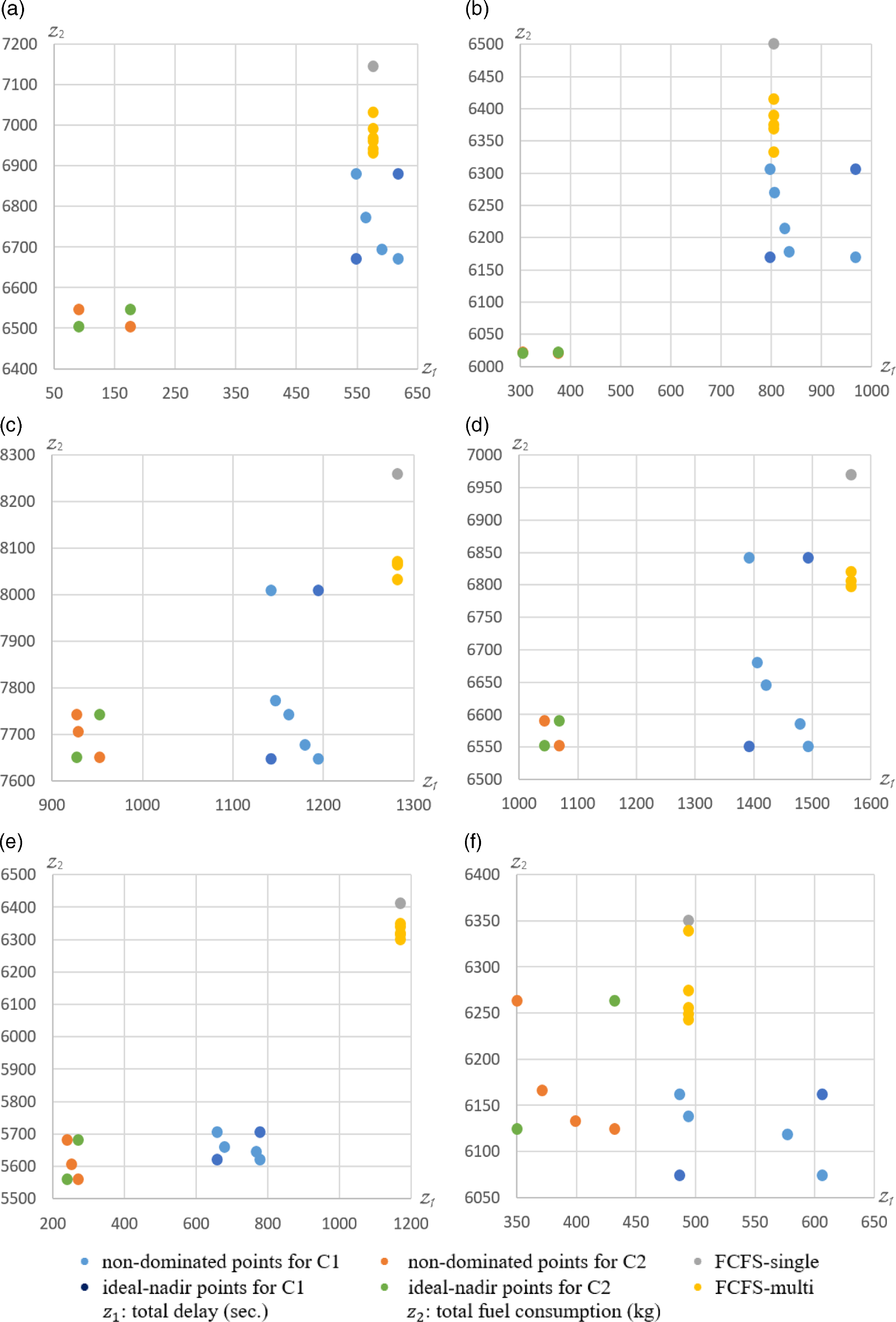
Figure 11. Results for traffic level of 22 aircraft.
All graphs show that the solution space narrows down in some scenarios for C2 compared to C1. However, almost all solutions obtained in C2 have lower total delay and fuel values when compared to solutions obtained in C1. Therefore, total delay and fuel are reduced when we allow departures to perform their operations before REP time. When we look at the non-dominated points compared to FCFS results, it is seen that total fuel is compromised in case of better total delay, while the total delay is compromised in case of better total fuel. There are also non-dominated solutions where both total fuel and total delay are better, according to FCFS results. When the primary objective was total fuel, the arrivals became the primary operations according to departures. In this case, the number of delayed departures increased while the number of delayed arrivals decreased. For example, in non-dominated results of C1 in Fig. 9(b), the number of delayed arrivals is 4, 3, 2 and 1 from left to right, while the number of delayed take-offs is 4, 5, 5 and 6. Therefore, the leftmost non-dominated solution point in graphs corresponds to minimum delay, while the rightmost non-dominated solution point corresponds to minimum fuel.
Figure 12 shows the average total delay of aircraft in all TL scenarios for C1 and C2. According to the figure, the average total delay in C2 was reduced by 23.2%, 49.6%, 35.9% and 43.9% compared with the C1 for 16, 18, 20 and 22 TL scenarios, respectively. This means that the number of delayed aircraft decreased when we allowed the departure aircraft to perform their operations before the REP time.
In order to compare the results of FCFS with non-dominated solutions of scenarios for C1 and C2, the percent improvement rates in total delay were calculated as given in Table 10. The percent improvement rates in total delay is equal to the percent ratio of the difference between the value of the objective in the FCFS approach and the value of the objective in obtained non-dominated solution to the FCFS approach. The values in the table show average, minimum and maximum improvement rates at each TL. Accordingly, the average total delay was reduced by 8.7% and 44% compared with FCFS for all TL runs in C1 and C2, respectively. These percentages correspond to an average of 73.7 and 372.6s for each run. In addition, when the maximum values are considered, it is seen that significant improvement in total delay have been achieved. The average values of maximum rates were 51% and 78.9% for all TL runs in C1 and C2, respectively. These percentages correspond to an average of 431.9 and 668.2s for each run.
The average total fuel of arrivals and departures in all TL scenarios for C1 and C2 is given in Fig. 13. According to the figure, the average total fuel of arrivals is close to each other in C1 and C2. There are small decreases in C2 except for 20 TL scenarios. When the total fuel of departures is compared, there has been a decrease in C2. This is a result of both a decrease in the number of delayed aircraft and a reduction in the delay duration of some individual aircraft. When the total fuel of the arrivals and departures is considered, it is lower in C2 than in C1.
We also compared the total fuels of non-dominated solutions with FCFS results and calculated average percent improvement rates in total fuel as given in Table 11. The values show average improvement rates compared to FCFS results of six different scenarios at each TL. The percent improvement rates in total fuel of non-dominated solutions compared to the FCFS-single approach are given as “FCFS-single”, while the improvement rates in total fuel of non-dominated solutions compared to the FCFS-multi approach are given as “FCFS-multi”. Accordingly, the percent improvements in total fuel of FCFS-single are higher than the FCFS-multi. The reason for this is that the model generates optimal trajectories using VMs while minimising both objective functions simultaneously. The model also generated optimal trajectories when it was run with the FCFS-multi approach. Therefore, the non-dominated solutions were compared with both FCFS-single and FCFS-multi results.
Table 10. The percent improvement rates in total delay for C1 and C2


Figure 12. Total delay (s).
As shown in Table 11, the average total fuel was reduced by 4.4% and 5.8% compared with the FCFS-multi for all TL runs in C1 and C2, respectively. These percentages correspond to an average of 268 and 353.3kg for each run. On the other hand, the average total fuel was reduced by 6% and 7.3% compared with FCFS-single for all TL runs in C1 and C2, respectively. These percentages correspond to an average of 372.5 and 453.2kg for each run. Note that these savings are only for a half-hour operational period on a single runway. These results indicate the importance of aircraft sequencing and scheduling considering the aircraft manoeuvres and flight profiles together at major airports within the TMA.
Table 11. Average percent improvement rates in total fuel
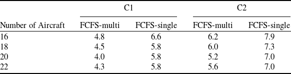
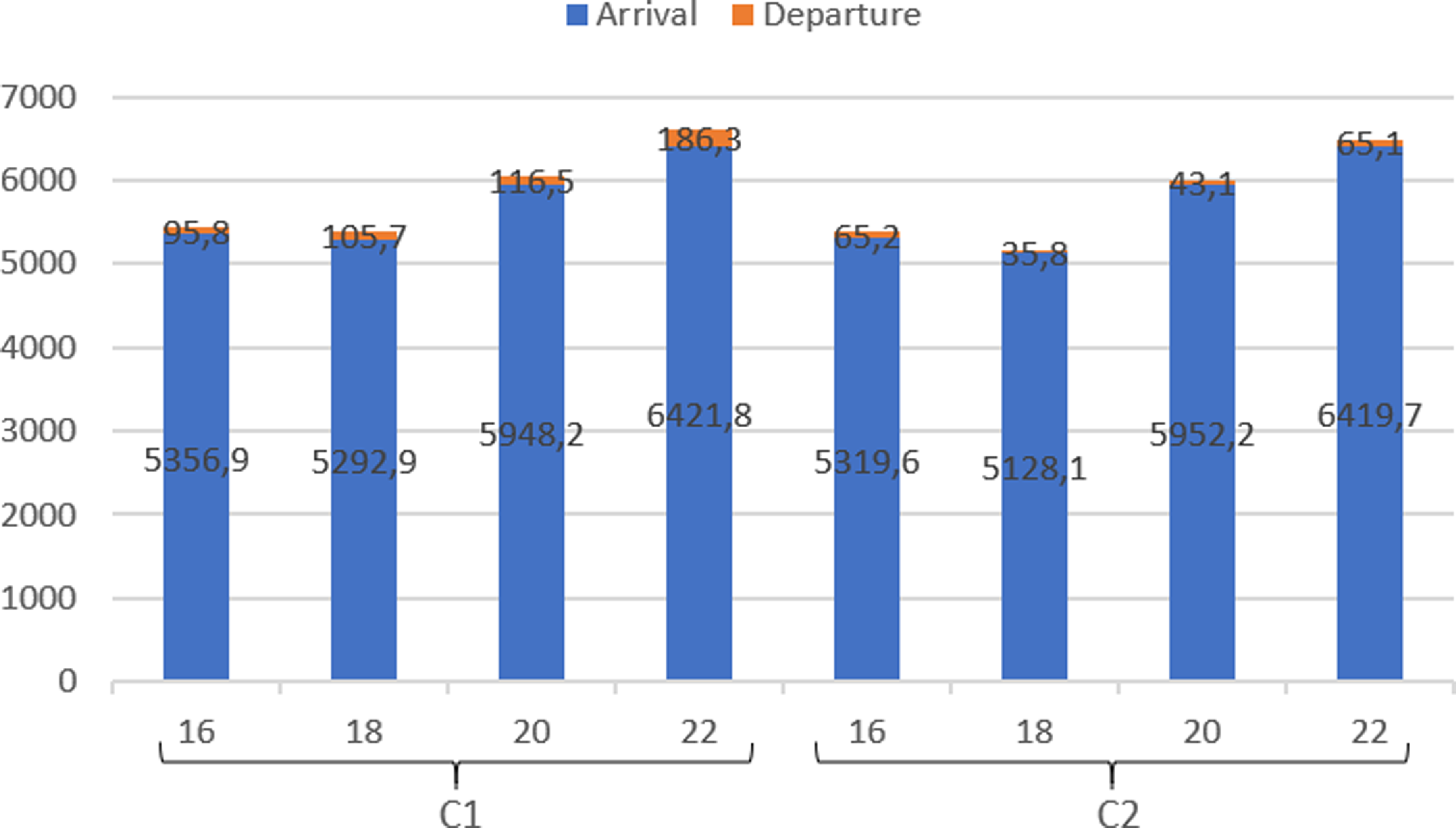
Figure 13. Total fuel (kg).
The runs with maximum improvement in total delay are determined for C1 and C2. The corresponding improvement in total fuel are also estimated for the same runs. In C1, the maximum decrease in total fuel for 16, 18, 20 and 22 TLs are 16.2%, 9.5%, 14.2% and 11.3%, respectively. In C2, the maximum decrease in total fuel for 16, 18, 20 and 22 TLs are 18.9%, 9.1%, 16.7% and 12.3%, respectively.
The runs with maximum improvement rates of non-dominated solutions can be seen in Fig. 8(e), 9(b), 10(e) and 11(e). We also selected these runs as an example to give more detailed information about the number of delayed aircraft and fuel of arrivals within the TMA. Table 12 shows the average number of delayed aircraft for non-dominated solutions in runs with maximum improvement rates. Accordingly, the total number of delayed aircraft in non-dominated solutions decreased according to FCFS. When we compared C1 and C2, there was a significant decrease in the number of delayed departures. Although there was an increase in the number of delayed arrivals in 16 and 18 TL scenarios, the total number of delayed aircraft decreased. This resulted in more decrease in the total fuel of aircraft in C2, as stated earlier.
Table 13 shows the total fuel of delayed arrivals during VM, while Table 14 shows fuel during level flight at EP level and FAF altitude in the same runs. The fuel given in Table 13 is directly proportional to the number of delayed aircraft given in Table 12. As the number of delayed aircraft decreased, the total fuel of VM decreased. The total fuel of aircraft during VM decreased significantly compared to FCFS in non-dominated solutions. According to the average values in the table, the percent improvement rate increased to 62% for 18 TL in C1 compared to FCFS-multi. The percent improvement rates were 48.1%, 27.2% and 35.2% for 16, 20 and 22 TLs, respectively. Accordingly, the total fuel of FCFS-single during VM is higher than FCFS-multi. The reason for this is that the proposed model generates optimal trajectories using VMs while minimising both objective functions simultaneously.
Table 12. The average number of delayed aircraft

Table 13. Fuel during the VM (kg)

Table 14. Fuel during level flights (kg)

When we examined total fuel during level flight given in Table 14, there was an increase in fuel at the TMA EP level according to FCFS, while a decrease in fuel at FAF altitude was observed. It is proof that this model allows aircraft to fly longer time at higher flight levels to achieve a fuel-optimal flight profile. Flying for less time at FAF altitude, it enabled the aircraft to make a fuel-optimal CDA approach.
In order to evaluate the effectiveness and practicality of the model in real-world situations, it was also tested with actual TMA operation data from LTFJ including 22 aircraft for a half-hour operational period. This data was selected from the 15:00–16:00 time zone with busy traffic on August 18 [63]. The calculated total delay and total fuel values for this reference day data are 555s and 7,446.1kg, respectively. These results are considered as the results of “baseline” scenario. Figure 14 shows the non-dominated solutions obtained with the proposed model for this scenario in C1 and C2. The solution times of the scenario for C1 and C2 are 227 and 98s, respectively. The results of baseline scenario are compared with the obtained non-dominated solutions for C1 and C2, and the percent improvement rates in the total delay and total fuel are given in Table 15. An improvement rate of up to 12.6% in total delay was achieved for C1, while up to 36.9% improvement was accomplished for C2. The improvement rates of total fuel range from 15.8% to 18.4% with an average of 17.4% for C1, whereas for C2, the rates range from 17.2% to 17.8% with an average of 17.5%. As the improvement rate in fuel consumption increases in non-dominated solutions, it results in an increase in total delay. The total delay is higher than the total delay in the baseline scenario in non-dominated solutions 3 and 4, where the total delay is shown with negative sign. The reason for this is that aircraft are kept on the ground for a longer duration to further improve the total fuel consumption of all operations.
Table 15. Percent improvement rates in the total delay and total fuel for real data

Table 16. Average computation times of non-dominated solutions (s)


Figure 14. Results for actual operation data.
The improvement rates in total fuel for baseline scenario based on the real operation data of LTFJ are greater than the improvement rates obtained in the test data results given in Section 4.3. The reason for this is that aircraft perform CDA in the study, while in the actual operation data they perform step-down approaches. Thus, in the study, they reach the runway with fewer level-offs (only at the FAF level) within the TMA. Compared to a step-down approach, CDA eliminates level segments by keeping aircraft at a higher altitude and reducing the need for additional thrust during descent. This results in lower fuel consumption.
4.4 Computation times
For each TL used in the study, the average computation times of solutions are given in Table 16. Accordingly, the computation time increases with the number of aircraft. In C1, the average solution time is almost 1 min. for 16 TL and less than 2, 3 and 5min. for 18, 20 and 22 TLs, respectively. In C2, the average solution time is less than 1min. for 16 TL, less than 2min for 18 TL, and less than 3min for 20 and 22 TLs.
5.0 Conclusion
In this study, a more realistic sequencing model with the multi-objective approach was developed in which both the total delay in air and on the ground and total fuel were minimised for arrival and departure mixed operations. By using the developed model, these two conflicting objectives were brought together, and non-dominated solutions were obtained. The $\varepsilon$
-constraint method was used and the total delay was added as a constraint to the model. This model can support current and developing automation of decision-support systems for enhanced airport operations, as well as focusing on the interest of different stakeholders such as airlines and ANSPs. A decision-maker can identify the most desirable solution among the non-dominated solutions.
$\varepsilon$
-constraint method was used and the total delay was added as a constraint to the model. This model can support current and developing automation of decision-support systems for enhanced airport operations, as well as focusing on the interest of different stakeholders such as airlines and ANSPs. A decision-maker can identify the most desirable solution among the non-dominated solutions.
Unlike the previous studies in the literature, a model including fuel cost function based on airspeed, altitude, bank angle and aerodynamic characteristics of the aircraft is presented here to represent the real-world problem more accurately. With VM and fly-by-turn defined within the scope of the study, the reality ratio is increased.
In the study, one aircraft type was selected for each wake-turbulence category, considering the aircraft coverage at LTFJ airport. In the mathematical model, all parameters are defined for each aircraft i. For this reason, more aircraft types for each wake-turbulence category can be adapted to the model. This does not require any changes to parameter definitions, only the number of parameters given to the model will change. Consequently, the model presented in the study has the ability to generate solutions for more than three aircraft types without significant changes in solution times.
We have shown that the proposed model always provides better solutions compared to the FCFS approach and provides the best results for all samples in 16, 18, 20 and 22 TL scenarios. Our findings show that the model reduces total delay and total fuel by up to 56.5%, and 16.2%, respectively, when compared to FCFS approach. These percentages correspond to 478.5s and 1,005.8kg. Also, allowing departures to perform their operations before estimated REP time has further reduced total delay and total fuel by up to 84.2% and 18.9%, respectively, compared to the FCFS approach. These percentages correspond to 713.1s and 1,173.4kg. Note that these savings are only for a half-hour operational period on a single runway of an airport within the TMA. These results indicate the importance of aircraft sequencing and scheduling considering the aircraft manoeuvres and flight profiles together at major airports.
To evaluate the practicality and effectiveness of the model in real-world scenarios, it was tested using actual TMA operation data from LTFJ, including 22 aircraft for a half-hour operational period. The improvement rates in total fuel for the baseline scenario, based on the real operation data of LTFJ, were found to be greater than the improvement rates obtained from the test data results. This is due to the fact that in the study, the aircraft perform CDA, whereas in the actual operation data, they perform step-down approaches. With CDA, the aircraft reach the runway with fewer level-offs (only at the FAF level) within the TMA, as compared to step-down approaches. This eliminates level segments by keeping the aircraft at a higher altitude and reducing the need for additional thrust during descent, resulting in lower fuel consumption.
Acknowledgements
This research received no specific grant from any funding agency in public, commercial or non-profit sectors.


