


Introduction
Studies have shown that even developed countries, like the U.S., face water challenges due to problems associated with affordability, demographic changes, high environmental quality expectations, and aging infrastructure (Wescoat, Headington, and Theobald Reference Wescoat, Headington and Theobald2007; OECD 2016; Allaire, Wu, and Lall Reference Allaire, Wu and Lall2018; Allen et al. Reference Allen, Clark, Cotruvo and Grigg2018). Examining affordability concerns, Mack and Wrase (Reference Mack and Wrase2017) project increasing water affordability issues with raising water rates, particularly in the state of West Virginia, where the highest percentage of at-risk census tracts (46 percent) for households unable to afford water bills of any state in the nation.
Aging water infrastructure, coupled with major funding shortfalls, is threatening the nation's water security (Alfredo et al. Reference Alfredo, Allaire, Becker, Boyle, Cho, Deane, Diserio, Lall, Lehman, McClain, Mucciacito, Pal, Pinero, Polycarpou, Sarni, Seidel, Yu, Yip and Weiss2016).Footnote 1 Many of the pipes and main lines that deliver water across the country are more than 100 years old and subject to a variety of stressors (American Society of Civil Engineers [ASCE] 2017). Aging water infrastructure leads to increased rates of main breaks, which result in water quantity and quality problems due to leaks and flowing contaminants into the water supply. An estimated 40 percent of the water distribution network's valves in the U.S. are not functioning properly (Baird Reference Baird2011). According to the ASCE (2017), an estimated 240,000 water main breaks occur every year, resulting in wastage of over two trillion gallons of treated drinking water. In terms of quality, previous research has linked water system deficiencies (e.g., loss of pressure caused by main breaks or maintenance work) to an increase in the flow of contaminants, resulting in more gastrointestinal illness incidents among the exposed households (Nygård et al. Reference Nygård, Wahl, Krogh, Tveit, Bøhleng, Tverdal and Aavitsland2007; Ercumen, Gruber, and Colford Reference Ercumen, Gruber and Colford2014).
The costs associated with replacing outdated water infrastructure are large. The American Water Works Association (2012) has estimated that $1 trillion in water infrastructure just needs to maintain the current levels of water service over the next 25 years. West Virginia, being one of the most rural states in the country, faces many challenges related to water supply reliability due to aging or non-existent water infrastructure (Levêque and Burns Reference Levêque and Burns2018). Statewide, there have been an increasing number of boil water notices (BWNs) related to water main breaks and other contamination episodes. The West Virginia Infrastructure and Jobs Development Council (WVIJDC 2017) has estimated that $17 billion is needed to connect all state residents to public water and to rehabilitate the existing water infrastructure.
Most of the needed improvements in water infrastructure are funded by local governments and public water system revenues generated by ratepayers (ASCE 2017). Since it is not optimal for a water system to achieve 100 percent reliability, decision makers need to make decisions that require trade-offs between cost and risk (Howe et al. Reference Howe, Smith, Bennett, Brendecke, Flack, Hamm, Mann, Rozaklis and Wunderlich1994). The required investment costs are usually known, but the risk preferences of the affected consumers are not. A large literature exists that examines consumers' willingness to pay (WTP) for different levels of public water supply reliability (e.g., Howe et al. Reference Howe, Smith, Bennett, Brendecke, Flack, Hamm, Mann, Rozaklis and Wunderlich1994; Griffin and Mjelde Reference Griffin and Mjelde2000; Koss and Khawaja Reference Koss and Khawaja2001), with the majority of these studies using stated preference approaches to conduct their analyses in developing countries. Other studies, using the revealed preference approach (averting behavior), have found that an unreliable water supply can also alter consumer behavior, leading to additional costs to the affected households (e.g., Pattanayak et al. Reference Pattanayak, Yang, Whittington and Bal Kumar2005; Jakus et al. Reference Jakus, Shaw, Nguyen and Walker2009; Vásquez Reference Vásquez2012).
One previous study by Des Rosiers, Bolduc, and Thériault (Reference Des Rosiers, Bolduc and Thériault1999) has investigated the impact of public water system unreliability on housing prices. They used data for 800 housing transactions in Quebec City, Canada, between 1990 and 1991, where 23 public warnings were issued during the study period. Warnings were grouped into 17 spatial sectors, each of which experienced one or more warnings. Using ordinary least squares (OLS) regression, they found that warnings were capitalized into property values with an average duration of the warning period per sector as a dominant factor. Also, market segmentation suggests that higher-price property buyers are much more responsive to this issue, such that they experienced value losses between 5.2 percent and 10.3 percent of the mean sale price.
Since water service is location-specific, access to a reliable and safe water supply should be an important public infrastructure attribute in determining residential property values. Therefore, the objective of this research is to examine the impact of water supply unreliability on residential property values. We examine this impact using a hedonic property model and measure this unreliability with BWNs in Marion County, West Virginia. Since water service reliability has been found to vary with the sociodemographic characteristics of communities (see VanDerslice Reference VanDerslice2011) and external impacts on property values can vary depending upon residential values (Lang and Cavanagh Reference Lang and Cavanagh2018), we utilize a quantile regression approach to estimating the impact of water supply unreliability on residential values across the entire distribution of house prices. We find statistically significant, negative relationships for estimated price impacts that are not uniform across the distribution of housing prices. Specifically, we find that BWNs have a larger impact on medium- to low-priced houses compared with high-priced houses. These results demonstrate implications for water affordability that extend beyond just what percentage of income is spent on water service to include wealth generated in the value of home ownership.
The rest of this article is organized as follows. A background section describing the study is followed by a section that covers the theoretical aspect of this research that combines a hedonic property price model and defensive expenditures along with the empirical framework of spatial quantile regression. The next section examines the data utilized in analyses. The final two sections discuss the results and conclusions.
Background
Located in the north central region of West Virginia, Marion County is a largely rural county with a population of nearly 56,000 (Figure 1). The county encompasses an area of 312 square miles and contains two cities (Fairmont and Mannington) and nine towns. Fairmont is the county's seat and the most populated city in the county. According to the U.S. Census Bureau (2018), the median household income in Marion County is $48,158, which is about 10 percent higher than the West Virginia median, but 20 percent lower than the U.S. median. The largest employers in the county are Fairmont State University and Fairmont Regional Medical Center. There are about 19,839 owner-occupied housing units in Marion County with a median value of $110,100 (U.S. Census Bureau 2018). Based upon comparisons of Marion County house sale data gathered for this research with regional and national housing median price trends, the residential real estate market in this county was reflective of regional and national housing price trends and judged to be relatively competitive between 2012 and 2017.
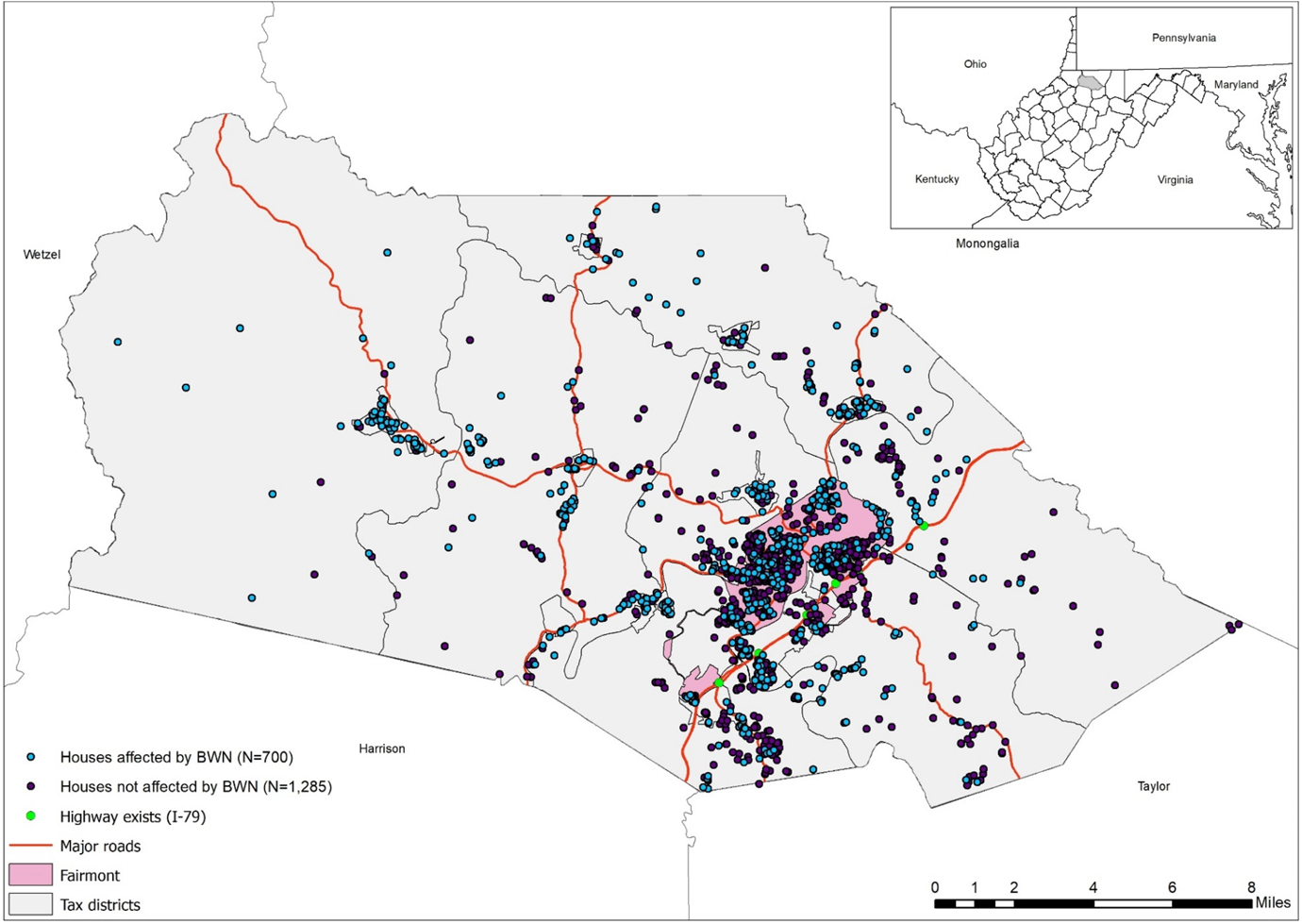
Figure 1. Residential Property Transactions Affected by Boil Water Notices in Marion County, West Virginia, Between 2012 and 2017.
Most of Marion County is served by the 28 public water systems located in the county—estimates include 95 percent of the population (USGS 2015) and 83 percent of structures (WVIJDC 2017). The city of Fairmont Water Department is by far the largest, serving over half of the county's population. Almost all public water systems in the county use surface water as source water, with only one system mixing ground and surface waters. Statewide in West Virginia, water systems with surface water sources have fewer violations than systems that utilize groundwater as a water source (U.S. EPA 2021).
One indication of problems with public water supplies is evidenced by water systems issuance of a BWN to alert their customers. A BWN, also known as a Boil Water Advisory, is issued when there is an identified or suspected microbial contaminant in the water distribution system. A BWN often occurs due to water main breaks. In Marion County, the reason for 80 percent of BWNs is water main breaks or leaks. Fixing a water main break, however, does not imply a lower likelihood in future breaks. In fact, the number of previous breaks is often reported as the most important factor for predicting future breaks (Pelletier, Mailhot, and Villeneuve Reference Pelletier, Mailhot and Villeneuve2003).
The BWN will instruct consumers to boil all water used for drinking, cooking, food preparation, brushing teeth, and making ice (Water Quality Research Foundation 2018). There are multiple methods of communications used to alert residents in the affected areas about BWNs, including local news, radio, newspaper, emails, texts, official websites, and door tags. In addition to the BWN, water system customers should be able to notice signs of a water main break from inside or outside their house. Inside a house, these signs include (1) low water pressure, (2) slowly flowing water, and (3) dirty water or a rusty discoloration, while outside a house, indicators include (1) water gushing or flowing from the ground, (2) sinking roads, sidewalks, or ground, and (3) water seeping or pooling out of the ground.
Marion County is among the top 10 counties in West Virginia that face major challenges related to water supply reliability based upon BWNs per 10,000 people. In addition, about 20 percent of the county's population are being served by public water systems that violated the health-based standards of the Safe Drinking Water Act (SDWA). Finally, 19 systems are designated as under-resourced (Public Service Commission of West Virginia 2017). These facts indicate that most water systems in Marion County are facing financial difficulties that may restrict service improvements and compliance with the SDWA standards.
Theoretical and empirical model development
Theoretical framework
The basic framework for the hedonic property price model was provided by Rosen (Reference Rosen1974), where consumers choose between differentiated products with multiple attributes to maximize their utility. In applying this model to housing markets, let Z = (z 1, z 2, …, z n) be a vector of observable attributes where z i measures the amount of the ith attribute of a house that includes property attributes (such as age, square footage, and number of bedrooms), neighborhood attributes (such as distance to schools and highways), and environmental attributes. Water supply unreliability (WSR) is included as a separate attribute that combines both neighborhood and environmental elements. Here, we assume that information about WSR is obtained by consumers of housing from BWNs that have been issued prior to the sale (BWN0).
Assuming a single competitive housing market and full information, the housing consumer decision problem is described as


where X is the numeraire good, WSR is a measure of water supply unreliability which is positively related to consumer expectations as derived BWN0, Y is income, P is the hedonic price schedule, and DE represents the associated defensive expenditures incurred (i.e., bottled water and water filter) when the water supply is unreliable so that (dDE)/(dBWN0) > 0.
Furthermore, we assume an expectation function:


where π represents a threshold on the number of BWN that housing consumers use when deciding whether water service provided to the house is deemed unreliable. When the number of BWNs issued prior to the sale is higher than π, then expectations of unreliable water supply are formed about the impacted property. Water supply unreliability will generate negative utility to the consumer, leading to a decrease in the price of the house.
Assuming that E(BWN0) > 0, the first-order conditions lead to:

Equation 5 shows that, at the optimum, the marginal implicit price of BWN0 from a hedonic property price model (RHS) reflects the marginal rate of substitution between water supply unreliability and the numeraire good X on the LHS along with a second term that measures the marginal change in defensive expenditures associated with BWN0 in order to achieve water supply reliability.
Rosen (Reference Rosen1974) also described the consumer's maximum ‘bid’ function for a house θ(Z;U, Y), where utility and income are fixed. This function represents the amount a consumer is willing to pay for different attribute vectors for a given utility–income index. Substituting the budget constraint into the utility function, we obtain:

If we implicitly differentiate θ( ⋅ ) with respect to BWN0, we obtain:

Combining conditions (5) and (7), we find that the marginal bid or the marginal WTP (MWTP) for a housing characteristic is equal to its equilibrium marginal price. The first-stage hedonic property price function P( ⋅ ) represents an envelope of a consumer's bid functions in equilibrium. Therefore, it can be used to obtain the marginal value that consumers place on housing attributes. This means that the marginal price of an attribute is equal to the MWTP for that attribute (Taylor Reference Taylor, Champ, Boyle and Brown2003). Econometrically, we obtain the marginal price of any attribute by regressing the price of the house on the attribute of interest, i.e.,BWN0 as a measure of WSR.
Empirical framework
Models stemming from the above theoretical framework could be estimated using OLS. However, recent studies adopt alternative estimation techniques to account for spatial dependence, i.e., the existence of a functional relationship between what happens at one location and what happens elsewhere (Anselin Reference Anselin2013). This issue may occur in hedonic property price models when houses in one location are impacted by the prices or characteristics of nearby houses compared with houses that are farther apart (Anselin and Lozano-Gracia Reference Anselin, Lozano-Gracia, Mills and Patterson2009). Also, spatial dependence may occur in hedonic property price models because of the presence of common practical issues such as measurement errors in explanatory variables, omitted variables, and other forms of model misspecification (Baumont Reference Baumont2004). Traditional OLS hedonic property price models do not consider the spatial dimension of housing price data, and ignoring spatial dependence may result in biased and inconsistent or inefficient estimates depending on the type of spatial process involved with the model (LeSage and Pace Reference LeSage and Pace2009).
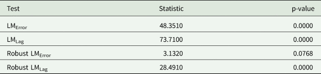
Therefore, spatial econometric techniques are used to address this problem and to obtain reliable coefficient and standard error estimates.Footnote 2 To address this, we account for potential spatial price spillovers using the spatial lag model as suggested by the Lagrange multiplier test results in Table 1. Thus, we can write the model as

where ln(P) is the natural log of the sale price, Z is a N × K matrix of property characteristics, B is a K × 1 vector of coefficients, W is a N × N spatial weight matrix associated with the autoregressive process in house prices and in the error term, and ɛ is a N × 1 spatial autoregressive error.
Table 1. Lagrange multiplier (LM) diagnostics for spatial dependence
A spatial weight matrix defines the relationship between neighbors in the model (i.e., how the value in one location in the system is affected by the values in other locations). This relationship can be based on either the distance or the contiguity between observations. For the spatial weight matrix, we use K-nearest neighbor (KNN) weights, in which all observations have the same numbers of neighbors (K) irrespective of the distance. This method is recommended to avoid the possibility of islands (i.e., observations without neighbors), which may result in loss of degrees of freedom, since all unconnected observations will be eliminated in the spatial model (Anselin and Bera Reference Anselin, Bera, Ullah and Giles1998). Also, this type of spatial weight matrix has been used frequently in other hedonic studies (e.g., Mueller and Loomis Reference Mueller and Loomis2008; Pandit et al. Reference Pandit, Polyakov, Tapsuwan and Moran2013; Netusil, Kincaid, and Chang Reference Netusil, Kincaid and Chang2014; Liu, Opaluch, and Uchida Reference Liu, Opaluch and Uchida2017). We also use a row-standardized weight matrix. For the number of neighbors K, we follow LeSage and Pace (Reference LeSage and Pace2009), and we choose the number that maximizes the value of a log-likelihood function. Using the log-likelihood function criterion, we find that using five nearest neighbors results in the maximum log-likelihood value.Footnote 3
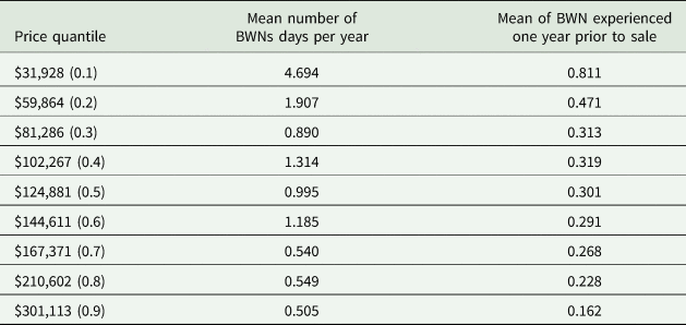
In our data, BWNs are not equally distributed across housing price transactions (Table 2). On average, properties transacted at the lower-price quantiles experience more water supply reliability problems than the properties sold at the higher-price quantiles. Therefore, we focus our analysis and look at the impact of water supply unreliability across the price distribution instead of assessing its impact with a focus on the mean. To do this, we employ the quantile regression approach (see Koenker and Bassett Reference Koenker and Bassett1978; Koenker and Hallock Reference Koenker and Hallock2001; Hao and Naiman Reference Hao and Naiman2007) to examine the impact of housing characteristics at different points (quantiles) across the distribution of housing prices.
Table 2. Boil Water Notices (BWNs) means by price quantile
Unlike OLS, quantile regression specifies changes in the conditional quantile, which allows us to observe how housing characteristics are valued differently by consumers of housing at different price ranges. Similar to equation 8, the spatial quantile lag model is expressed as

which will result in estimates based on the conditional quantile, taking account of the spatial effect at the same time.
To estimate the spatial quantile model, the two-stage quantile regression approach proposed by Kim and Muller (Reference Kim and Muller2004) is used to account for the endogeneity in the spatially lagged variable. In the first stage, the spatially lagged exogenous variables WZ and Z are used to predict the spatially lagged endogenous variable W ln(P) at an individual quantile. The predicted $\widehat{{W\,{\rm ln}( P ) }}$ is substituted for W ln(P) in the spatial lag model to eliminate the correlation between the spatially lagged endogenous variable and the error term. Then, the second-stage regression for that quantile is performed to obtain ρ(τ) and β(τ). This two-stage procedure is then repeated for each quantile.
Data
Our analysis is based on two main sources of data: (1) West Virginia Office of Environmental Health Services (OEHS) and (2) Marion County Assessor. The next two subsections provide descriptions of these data.
Boil water notices
To measure water supplier unreliability, we use BWNs issued by either public water systems or the Marion County Health Department. The OEHS provides information on all BWNs in West Virginia starting from 2012. Between January 2012 and December 2017, there were a total of 440 BWNs in Marion County, varying annually between 64 and 80 with no discernible trend over time. For each notice, the provided information includes the following: when the notice is issued and lifted, the name of the public water system plus its PWSID, the public health sanitation district where the notice is issued, the reason for the notice, and details about the affected areas or street names.Footnote 4 Using information from the SDWIS/Fed database and details from each notice, we obtained city and county affected by each notice.Footnote 5
Housing data
The Marion County Assessor provides data for all residential property sales between January 2012 and December 2017. This data set contains 7,972 residential property transactions. By dropping all property sales without structures, the number of transactions declined to 5,525. To ensure only arm's length sales in our analysis, a process following Herriges, Secchi, and Babcock (Reference Herriges, Secchi and Babcock2005) is used to drop all properties that were less than 50 percent of their assessed values and/or sold for less than $5,000. Therefore, after eliminating these sales, the total number of transactions included in our analysis is 1,985 single-family residential properties.Footnote 6
To capture housing attributes previously found in the literature to influence housing prices, we include variables for housing characteristics in the hedonic model such as size, story height, age, number of bedrooms, total number of bathrooms, and existence of house amenities (e.g., air-conditioning and fireplace). In addition, we control for two variables that have been consistently neglected in hedonic property price models: (1) house physical condition and (2) material and workmanship quality. Based upon assessor data for physical condition, we rank houses from Unsound = 1 to Excellent = 6. For quality, we use the quality grade factor provided by the county's assessor ranging from E = Poor (0.5) to X = Excellent (2.5). According to the assessor, these two variables are unrelated, as the first one measures only the physical condition, but the second measures the quality of the building regardless of the physical condition. We compute a simple correlation coefficient, and we find that it is equal to 0.60, indicating a moderate correlation between the physical condition and the quality of the building.
All property sales are geocoded using house's street address with ArcGIS to measure neighborhood and proximity characteristics such as crime, school quality, distance to Fairmont State University, and to the nearest highway interchange.Footnote 7 For crime, we use the total crime index that compares the average local crime level to that of the entire U.S. (an index of 100 is average). This index includes both property and violent crimes for 2010 at the block group level, and it is obtained from the ArcGIS database. For school quality, we follow the literature and use proficiency tests as a proxy (Brasington Reference Brasington1999). Specifically, we use the percentage of students in elementary school who scored at or above proficiency levels in math tests. We obtain these shapefiles for attendance zones in the county from the National Center for Education Statistics (NCES) and the data for math tests from the GreatSchools website. For distance variables, we obtain the shapefiles for Fairmont State University and highway interchange locations from the Census Bureau TIGER/Line database. Finally, we include year-fixed effects to control for housing market changes over time.
Linking BWNs to housing transactions
There were 440 BWNs in Marion County between 2012 and 2017, but 90 BWNs could not be used due to insufficient information about the affected locations (54 BWNs) or because the date when the BWNs were lifted are unavailable (36 BWNs). Thus, the total number of BWNs used in the analysis is 350. Then, based upon the details provided for each BWN along the street address for each property transaction, West Virginia Property Viewer was used to allocate properties and BWNs among the 22 tax districts in Marion County.Footnote 8 Following this, the details of each BWN are linked to all affected houses based on street addresses or affected areas. For example, if a BWN affects Street A and is issued on January 1, 2014 and lifted on January 5, 2014, houses located at Street A and sold between January 1, 2014 and January 1, 2015 are assigned the appropriate values for each BWN variable utilized in the analysis.
Table 3 shows the distribution of property transactions, BWNs, and properties affected by BWNs in each tax district in Marion County between 2012 and 2017. Over the entire county from 2013 to 2017, about 35 percent of residential property transactions are affected by a BWN, and as expected, Fairmont has the largest number of transactions and BWNs. Specifically, about 41.6 percent of the transactions happen in Fairmont with 29 percent of these transactions being affected by BWNs.
Table 3. Property transactions and BWNs by tax districts in Marion County, West Virginia, between 2012 and 2017
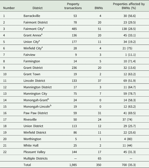
a Part of Fairmont City.
b BWNs that affect districts 14 and 15 usually affect other districts as well.
Two variables are used to measure water supply unreliability: (1) the number of days a sold house is under BWNs within one year prior to its sale date and (2) a binary variable indicating that if a sold house is affected by the BWN or not within one year prior to its sale date.Footnote 9 For these variables, property sales from January 1, 2013 to December 31, 2017 are used in the analysis and BWNs from January 1, 2012 to December 31, 2016.
Table 4 provides summary statistics and descriptions for all variables included in the analysis. Explanatory variables are grouped into four categories. The first category consists of focus variables related to BWNs as proxy measures of water supply unreliability. We expect these variables to have negative impacts on housing prices. The second category is structural variables that include building characteristics and house amenities. Except for story height, construction material, and house age, all the other variables are expected to have positive impacts on housing prices. Property variables are the third category, and these include parcel characteristics of lot size and fencing with positive impacts and sidewalks with a negative impact, since they are associated with cleaning responsibilities. Finally, there are neighborhood and proximity variables. For the variables crime level and distance to highway plus a major employer (Fairmont State University), negative impacts are expected, whereas school quality should have a positive impact on housing prices.
Table 4. Summary statistics and variable descriptions
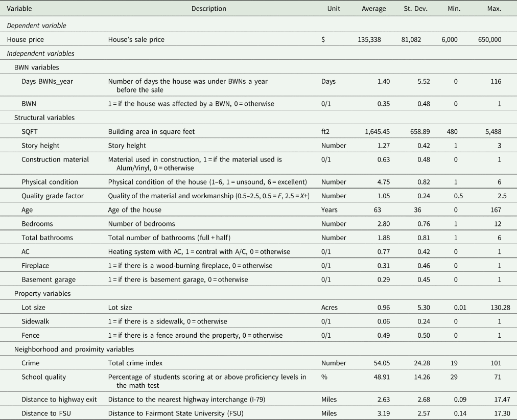
Note: Observations = 1,985.
Results
First, a single market assumption for residential properties in Marion County is confirmed from our data using a Chow test on models comparing two data subsamples: (1) the city of Fairmont and (2) the rest of Marion County. To examine the changing impact of water supply unreliability over the distribution of housing prices, the spatial quantile regression model results are reported in Appendix Tables A1 and A2. All estimates for the spatial autoregressive coefficient (ρ) are positive and statistically significant, meaning that a positive spatial similarity exists between residential property sale prices. Focusing on the BWN variables with coefficients statistically different from zero, it is clear from Table 5 that water supply unreliability has more negative impacts on house sales at the lower quantiles of the house price distribution compared with houses priced at the high quantiles. For example, the Days BWNs_year variable has negative, statistically significant impacts for quantiles between 0.1 and 0.6, but no statistically significant impacts at quantiles 0.7 or greater.
Table 5. Two stage least square (2SLS) estimates for the spatial quantile models (dependent variable is ln (P))
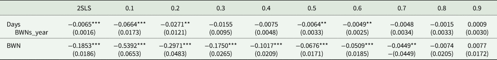
Note: Bootstrapped standard errors in parentheses.
***p<0.01, **p<0.05.
We also examine the valuation of water supply unreliability computed using the estimates from the first-stage hedonic property price model. As mentioned in the theory section, the MWTP is defined as the derivative of the hedonic price equilibrium equation with respect to the characteristics of interest. Following Muller and Loomis (Reference Mueller and Loomis2008) and Anselin et al. (Reference Anselin, Lozano-Gracia, Deichmann and Lall2010), the MWTP from the spatial lag model consists of a coefficient and a spatial effect because the impacts from a change in one household's water supply unreliability spill over to neighbors. Following Kim, Phipps, and Anselin (Reference Kim, Phipps and Anselin2003), the equation can be written as

where $\hat{{\rm \beta }}$ is the coefficient, $\bar{P}$
 is the mean housing price, and $\hat{{\rm \rho }}$
 is the estimated spatial autoregressive coefficient. This spatial multiplier effect needs to be accounted for to accurately compute the MWTP.
It is important to note that these marginal benefit estimates represent a capitalized rather than an annual impact from water supply unreliability. As such, the marginal benefit estimates are influenced by the length of time the buyer of the house expects to reside in the house, the amount the buyer expects to receive for this attribute when the house is resold, the discount rate, and any projected improvements in water infrastructure. Table 6 shows the MWTP calculations for the BWN variables with statistically significant coefficients from the estimated spatial models. As can be seen, on average, the MWTP for improving water supply reliability ranges from $1,160 to $35,116 depending upon how unreliability is measured—in either days or presence versus absence.
Table 6. MWTP ($) for a change in water supply reliability from the estimated spatial models

Notes: The values represent coefficients that are statistically significant at 5 percent; empty cells are for insignificant coefficients. Since BWN is a binary variable, its marginal impact is equal to: Mean P in quantile * (exp(b) − 1) * (1/1 − ρ).
Since the number of days in which the house is expected to be under BWNs over a year represents a clear and known marginal change, we use it as the preferred measure to value water supply unreliability. Thus, by reducing the expected number of BWN by one day per year per house, the total effect of this change, on average, would be an improvement by $1,160 in housing prices when including the impacted house itself and its neighbors. This impact represents 0.86 percent of the average house price in Marion County. This impact is more substantial than other neighborhood variables in the model such as crime and school quality (see Appendix Table A1 for coefficient estimates).
The average MWTP of $1,160 for a one-day reduction in the annual number of BWN is high, relative to the defensive expenditures involved. Daily household estimates from three studies that examined the economic costs of defensive expenditures due to potable water contamination (Harrington, Krupnick, and Spofford Reference Harrington, Krupnick and Spofford1989; Abdalla, Roach, and Epp Reference Abdalla, Roach and Epp1992; Collins and Steinbeck Reference Collins and Steinback1993) range from $3 to $20 in 2017 dollars. This compares with a capitalized defensive expenditure value of $70 per day from the average MWTP value.Footnote 10 There are several explanations for this large difference: (a) the spatial correlation impacts between houses impacted by the BWN that are embedded in the MWTP estimates, (b) enhanced risk perceptions of households impacted by the BWN as explained below, and (c) the capitalized defensive expenditure value may represent the cost of leaving the home temporarily while the BWN is in effect rather than the economic cost of in-house responses.
Furthermore, we see that the MWTP values for consumers of low-priced houses are greater than for consumers of high-priced houses. That is, a reduction of one day under BWN per year will increase housing prices at the medium to lower end of the housing price distribution by $2,100 to $2,700, whereas houses at the mid-range of the distribution will increase by $850 to $1,000 (Table 6). These impacts range from 0.60 percent to 8.4 percent of average sale prices across these quantiles. Houses at the 0.7 quantile and above of the price distribution show no statistically significant impacts from the days of the BWN variable. Finally, given the mean distribution of BWNs by quantile in Table 2, a threshold value (π) of approximately 1.0 BWNs annually is indicated by the statistically insignificant results at the 0.7 quantile and above.
One interpretation of these results is that the greater prevalence of BWN for lower-priced houses leads to greater risk perceptions and awareness about public water supply problems among these housing consumers. Previous studies have shown that consumers who experience more problems with their water supply perceive the associated health risks differently and were willing to pay more to fix water supply problems than those consumers who experience water supply problems infrequently (Anadu and Harding Reference Anadu and Harding2000; Genius and Tsagarakis Reference Genius and Tsagarakis2006). As shown in Table 2, experience with and duration of BWNs consistently declines with housing price quantiles.
Overall, water supply unreliability has a substantial impact on the value of residential properties in Marion County. To calculate the aggregate MWTP across the entire county for a one-day reduction of BWN, three factors are multiplied together: (1) the average value of statistically significant coefficients from the spatial quantile regression ($1,694), (2) the estimated annual average number of owner-occupied housing units that would be expected to be affected by the BWN in Marion County between 2013 and 2017 (6,150), and (3) finally, from the quantile regression results, a factor of 0.4 as the percentage of houses would incur a price impact from these notices. Following this procedure, we obtain an aggregate MWTP value of $4.2 million for a one-day reduction of the annual BWN throughout Marion County.
Conclusions
Aging water infrastructure, combined with funding shortfalls, poses serious challenges to local governments and water systems across the U.S. The number of water main breaks in the U.S. has been increasing every year resulting in more interruptions in public water service (Folkman Reference Folkman2018). Since achieving full reliability in water service is most likely not an optimal policy, decision makers at local water utilities must attempt to balance between cost and risk associated with their policies (Howe et al. Reference Howe, Smith, Bennett, Brendecke, Flack, Hamm, Mann, Rozaklis and Wunderlich1994). However, water customers’ perceptions of the risk associated with supply disruptions are usually unknown to decision makers. Therefore, studies have attempted to examine the WTP for water supply reliability using stated preference approaches (Genius and Tsagarakis Reference Genius and Tsagarakis2006; Vásquez and Espaillat Reference Vásquez and Espaillat2016).
In this research, we examine the impact of water supply unreliability on single-family, residential property sales in Marion County, West Virginia, using spatial quantile hedonic property price models. To measure the impact of water supply unreliability, we define two variables based on the issuance of BWNs within one year prior to the sale and link them to house sale transactions. Our analysis is based on 1,985 housing transactions and 350 BWNs throughout the county between 2012 and 2017. Important factors that affect observed house prices are controlled for by including house size, age, number of bedrooms plus bathrooms, construction quality, and existence of house amenities (air-conditioning, fireplace, and fence).
We find that there are statistically significant, negative impacts on house prices from prior issuances of BWNs. When unreliability is measured by days of BWNs, a one-day increase can depreciate housing prices at the margin from 0.6 percent to 8.4 percent. Furthermore, using a quantile regression approach, we find that water supply unreliability has a larger impact on medium- to low-priced houses compared with high-priced houses. Based on what we would judge as the best estimate of water supply unreliability, the MWTP for a reduction in one day under a BWN per year will increase house values at the lower end of the price distribution in the range of $2,100 and $2,700, whereas houses at the mid-range of the distribution will increase by $850 to $1,000. However, house transactions at the higher end of the housing price distribution show no statistically significant impacts from the days of the BWN variable. The conclusion that improving water infrastructure will increase property values is supported by previous research that examines the impact of public infrastructure investments on housing prices (Janeski and Whitacre Reference Janeski and Whitacre2014; McIntosh et al. Reference McIntosh, Alegría, Ordóñez and Zenteno2018).
The results from the quantile regression models can be interpreted as an inconvenience measure, where consumers are willing to pay to fix water supply reliability problems until a certain threshold in which after that point their MWTP will be zero. Our results indicate that consumers’ MWTP will be positive if the house is expected to experience, on average, one day or more under BWNs annually. Since many residences in Marion County (particularly medium- to low-priced houses) experience more than one day of BWNs, water supply unreliability has a substantial impact on the value of residential properties in this county (between 1 percent and 10 percent of the sale price). Given that the primary impacts from water supply reliability fall upon medium- to low-priced houses, this research result shows that affordability of public water service is an issue that not only involves the amount or percentage of income expended upon water services (Mack and Wrase Reference Mack and Wrase2017; Whittington Reference Whittington2020), but also entails service reliability and its impact on the wealth generated in housing values for low- to medium-priced houses.
Comparing our BWN impact estimate with the results of Des Rosiers, Bolduc, and Thériault (Reference Des Rosiers, Bolduc and Thériault1999), we note that these authors found a larger magnitude of impact for BWNs. This difference is to be expected since we are using a larger sample size and a different methodology of linking BWNs to sale observations. For linking BWNs to sale observations, they used aggregated measures and grouped the BWNs into multiple “spatial sectors” where each of them had one or more warnings, and any house that was located in those sectors was considered having problems with water quality. On the other hand, we use specific measures for each house as explained in the subsection linking BWNs to housing transactions.
Our estimates indicate that some households in Marion County have a positive MWTP for a greater reliability in their water supply. This research demonstrates, via these enhanced housing values, the public desirability of addressing water infrastructure needs of lower- to middle-income communities through federal programs such as the American Jobs plan. In addition, the aggregated value for the MWTP of $4.2 million to reduce the BWN by one day may help guide and motivate water systems in their decisions regarding water pricing and investments in the water distribution network. With its negative impact on property valuation, property tax revenues collected by the county are potentially reduced due to unreliable water supplies.
Finally, it is important to note, however, that our findings reflect the specific nature of our data. The area of study is a relatively small geographical area. Also, due to missing data, we had to drop a relatively large number of BWNs (90) from our analysis. In addition, when allocating BWNs to house sale observations, most BWNs affect one or multiple streets in addition to surrounding areas. Due to our limited knowledge, we were unable to include those surrounding areas in our analysis. Therefore, not all of the house sale transactions affected by the BWN were included in this analysis. Against this background, our monetary estimates of BWN impacts should be regarded as conservative.
Data availability statement
All data are available on public databases.
Funding statement
This research received no specific grant from any funding agency, commercial, or not-for-profit sectors.
Conflicts of interest
None declared.
Appendix
Spatial quantile regression models—dependent variable is ln (P)
Table A1. Spatial quantile regression results for model (1)—days BWNs_year
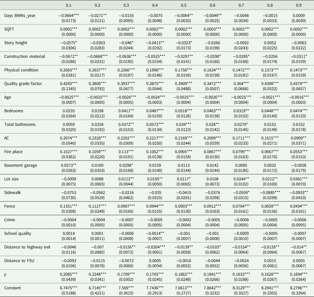
Table A2. Spatial quantile regression results for model (2)—BWN

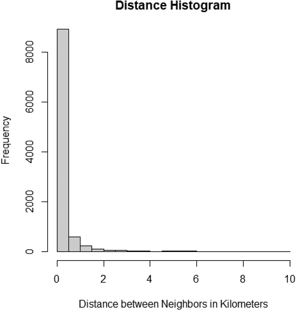
Figure A1. Distance Histogram Between Neighbors in the Weight Matrix.


 Open access