


1. Introduction
So-called compartment models play an extensive role in the mathematical modeling of the spread of an infectious disease in epidemiology. They describe the size of a population in a specific state relating to the evolution of the disease, for instance, Susceptible, Infected, and Recovered in the canonical SIR model. Generalized models may include states for Hospitalized or Dead. If the state Recovered also covers being Immune, one may, e.g., not need a specific state for vaccinated since the occurrence of vaccination may be formalized as a transition from susceptible to immune without having been Infected in between. This is just an example of how one can play with the compartment models and the transitions to capture what is considered essential for a given situation.
The compartment models are introduced as deterministic models, and the number of individuals in the different states is described via a deterministic system of differential equations. One way of including uncertainty is to add noise to these deterministic differential equations, such that the number of individuals in a given state in a population is modeled as a stochastic differential equation. A general introduction to compartment models is found in Keeling (Reference Keeling2008).
We take a different route. When the number of individuals in the various states is divided by the total number of individuals in the population, new differential equations describe the proportion, also deterministic, of the people in the different states. We view them instead as probabilities for an arbitrary individual in the population being in the various states. In this case, the system of deterministic differential equations can be viewed as Kolmogorov’s forward differential equation. From this system, we can then detect the intensities of the underlying stochastic Markov model. In particular, we can study how these intensities incorporate the impact of contagion by being dependent on the transition probabilities. There it becomes clear that we need to work with time-inhomogenous Markov models.
The initial distribution used in Kolmogorov’s differential equation is set to the initial proportion of individuals in the states, corresponding to an arbitrary individual being in the specific state at the initiation. We can marginally follow a particular individual in the Markov model for whom we know the initial state based on the intensities of the population’s initial condition. We can calculate transition probabilities and other relevant quantities. The individual transition probabilities deviate from the population transition probabilities only by the initial condition in the differential system.
For an individual, we can introduce insurance contracts relating to the risks, individual payment streams relating to sojourns in or transitions between states, and individual reserves based on conditioning on the individual being in a specific state, all related to the underlying Markov model.
The object of this study is two-fold. First, we show how the deterministic differential equation can be viewed as Kolmogorov’s equations and identify the structure of its intensity function. This is a purely probabilistic object. The stochastic pattern of thinking opens a box of potentially interesting quantities to study relating to the uncertainty of the system, e.g., the variance of a specific or arbitrary individual being in a given state. Also, studying the longer-term distribution/risk of the stochastic model is interesting to understand the meaning of an epidemic to end. It is beyond the scope of this paper to explore this box. The first object is to open it. Second, we want to study insurance contracts, payment streams, and reserves with a classical individual approach based on the underlying Markov model and the attached intensities.
The first object relates to other studies introducing stochastic elements in the deterministic compartment models. Various models may overlap depending on which noise is added and how this noise is added to the deterministic differential equations. Related to our work, Lefèvre & Picard (Reference Lefèvre and Picard2018) and Lefèvre & Simon (Reference Lefèvre and Simon2020) also model the evolution of an epidemic in a population via a Markov model. The particular block structure of their Markov model allows for efficient calculation of various objects of interest. Our Markov model can be viewed as a certain mean-field approximation to the Markov model studied in Lefèvre & Picard (Reference Lefèvre and Picard2018) and Lefèvre & Simon (Reference Lefèvre and Simon2020), and we comment on that relationship in a separate subsection. The textbook (Britton & Pardoux, Reference Britton and Pardoux2019) also presents the Markov model point of view similar to the one taken by Lefèvre & Picard (Reference Lefèvre and Picard2018) and Lefèvre & Simon (Reference Lefèvre and Simon2020). Common for all of them is that their starting point is a Markov model on the population level, whereas our starting point is the individual level. These different starting points give different routes, and identifying individual-level Kolmogorov’s equations with transition probability-dependent intensities is our work’s significant and exclusive contribution. The studies in Lefèvre et al. (Reference Lefèvre, Picard and Simon2017), Lefèvre & Simon (Reference Lefèvre and Simon2022), Lefèvre & Picard (Reference Lefèvre and Picard2018), and Lefèvre & Simon (Reference Lefèvre and Simon2018) relate to ours by also clicking contagion risk from epidemics to insurance and risk management. In Lefèvre & Picard (Reference Lefèvre and Picard1993) and Picard & Lefèvre (Reference Picard and Lefèvre1993), the fatal risk is studied, corresponding to when we introduce death in our model. Finally, we mention Hillairet & Lopez (Reference Hillairet and Lopez2021) for integrating compartment models in a non-life risk approach to cyber risk. See also Boado-Penas et al. (Reference Boado-Penas, Eisenberg and Şahin2021) for further relations between insurance risk and pandemics.
The second object is to study the impact of infection on individual reserves in life and health insurance. This is closely related to Feng & Garrido (Reference Feng and Garrido2011) and Feng et al. (Reference Feng, Garrido, Jin, Loke and Zhang2022), also implementing the population dynamics of epidemic models into the context of life insurance much in line with what we do. However, they always take the population perspective and do not recognize and use the state model from an individual’s perspective. This population perspective spills over when introducing reserves such that all calculations remain on a population level and no individual reserves are considered. We study the relationship between the notions of reserves arising from their work and ours.
The paper’s outline is as follows: Section 2 introduces the canonical SIR compartment model as an example of a compartment model. Section 3 starts by relating the SIR compartment model to a specific three-state Markov model with transition probability-dependent intensities. After that, we generalize the structure to general time-continuous time-inhomogenous finite-state Markov models. In Section 4, we use the available setup studied in Section 3 to add a death state and form the Markov model related to the so-called SIRD compartment model. Section 5 introduces insurance contracts, individual reserves, and population reserves. We formalize and illustrate the relationship to the models and numerical results in Feng & Garrido (Reference Feng and Garrido2011) and extend the model and numerical results with further aspects arising from the experience of the coronavirus.
2. The Dynamics of an Infectious Disease
When modeling an infectious disease, it is essential to keep track of the infected people in the population. They have contracted the disease, are sick, and may transmit it to others. The immune system eventually fights off most infections, though. The recovered individuals are no longer infectious; in most cases, they have developed some immunity against the disease. Only the people without immunity can contract the disease and are, thus, susceptible to the disease.
A classical, epidemiological way is to categorize each individual in the population as susceptible, infectious, or recovered. It is possible to add more labels to refine the stages of an epidemic model; see Section 3.2. The number of individuals in each category is modeled with an epidemiological compartment model. The simplest and most well-known model is the SIR model. It consists of three compartments called $S$
,
$S$
, $I$
, and
$I$
, and $R$
, representing the susceptible, infected, and recovered individuals, respectively. Let the functions
$R$
, representing the susceptible, infected, and recovered individuals, respectively. Let the functions $S(t)$
,
$S(t)$
, $I(t)$
, and
$I(t)$
, and $R(t)$
denote the number of individuals in each compartment at time
$R(t)$
denote the number of individuals in each compartment at time $t$
. Note that the simple SIR model assumes that all infected individuals eventually recover, although some people might die from the disease. However, from an epidemiological viewpoint, being dead and being recovered are equivalent because you are neither susceptible to nor carrying the disease. The literature often combines them into one compartment and calls them removed if the immunity is life-long. The SIR model is one of the simplest models to illustrate epidemic behavior.
$t$
. Note that the simple SIR model assumes that all infected individuals eventually recover, although some people might die from the disease. However, from an epidemiological viewpoint, being dead and being recovered are equivalent because you are neither susceptible to nor carrying the disease. The literature often combines them into one compartment and calls them removed if the immunity is life-long. The SIR model is one of the simplest models to illustrate epidemic behavior.
The simple SIR model describes the dynamics of the epidemic, i.e., how individuals move from compartment to compartment. As seen in Fig. 1 which illustrates the SIR model, it is possible to go from compartment $S$
to
$S$
to $I$
at time
$I$
at time $t$
with the Force of Infection
$t$
with the Force of Infection $\lambda (t)$
, which is defined as the per capita rate at which susceptible people contract the infection. The total number of new infections in a small time interval,
$\lambda (t)$
, which is defined as the per capita rate at which susceptible people contract the infection. The total number of new infections in a small time interval, $[t,t+dt)$
, is then
$[t,t+dt)$
, is then $\lambda (t) S(t) dt$
. The move from compartment
$\lambda (t) S(t) dt$
. The move from compartment $I$
to
$I$
to $R$
happens with the per capita recovery rate
$R$
happens with the per capita recovery rate $\gamma (t)$
, and the total number of recoveries in a small time interval,
$\gamma (t)$
, and the total number of recoveries in a small time interval, $[t,t+dt)$
, is then
$[t,t+dt)$
, is then $\gamma (t) I(t) dt$
. The rate
$\gamma (t) I(t) dt$
. The rate $\gamma$
is, in simple models, assumed to be constant.
$\gamma$
is, in simple models, assumed to be constant.

Figure 1. The simple SIR model. It shows how people in the population move through the susceptible ( $S$
), infectious (
$S$
), infectious ( $I$
), and recovered (
$I$
), and recovered ( $R$
) stages of an infectious disease. The transition from compartment
$R$
) stages of an infectious disease. The transition from compartment $S$
to
$S$
to $I$
at time
$I$
at time $t$
happens with intensity
$t$
happens with intensity $\lambda (t)$
, and the transition from compartment
$\lambda (t)$
, and the transition from compartment $I$
to
$I$
to $R$
at time
$R$
at time $t$
happens with intensity
$t$
happens with intensity $\gamma (t)$
.
$\gamma (t)$
.
One central question is how to model the Force of Infection $\lambda (t)$
. It depends on two factors; how prevalent the disease is in the population and how it is transmitted. There must be contact between susceptible and infected individuals for directly transmitted diseases. Let
$\lambda (t)$
. It depends on two factors; how prevalent the disease is in the population and how it is transmitted. There must be contact between susceptible and infected individuals for directly transmitted diseases. Let $c(t)$
be the contact rate, i.e., the intensity of contacts in the population. It may change over time, e.g., if a lockdown is declared. Let
$c(t)$
be the contact rate, i.e., the intensity of contacts in the population. It may change over time, e.g., if a lockdown is declared. Let $p(t)$
be the probability of transmitting the disease upon contact. This changes if preventive measures are applied, e.g., protective equipment, face masks, and disinfectants. Combining these rates gives the transmission rate, which is defined as
$p(t)$
be the probability of transmitting the disease upon contact. This changes if preventive measures are applied, e.g., protective equipment, face masks, and disinfectants. Combining these rates gives the transmission rate, which is defined as $\beta (t) = p(t)c(t)$
. Furthermore, the proportion of the contacts that are infected must be taken into account. Let
$\beta (t) = p(t)c(t)$
. Furthermore, the proportion of the contacts that are infected must be taken into account. Let $N=S(t)+I(t)+R(t)$
denote the population size, which is assumed constant in the simple SIR model. This is a reasonable assumption when looking at relatively short epidemics or a single outbreak. The short time horizon makes the epidemic dynamics dominate the impact of demographic changes.
$N=S(t)+I(t)+R(t)$
denote the population size, which is assumed constant in the simple SIR model. This is a reasonable assumption when looking at relatively short epidemics or a single outbreak. The short time horizon makes the epidemic dynamics dominate the impact of demographic changes.
The prevalence of infection in the population is given by $\frac{I(t)}{N}$
. Combining the prevalence with the transmission rate, we can define the Force of Infection as follows:
$\frac{I(t)}{N}$
. Combining the prevalence with the transmission rate, we can define the Force of Infection as follows:
 \begin{align} \lambda (t) = \beta (t) \frac{I(t)}{N}. \end{align}
As mentioned, this is the per capita rate at which susceptible individuals contract the infection. The total number of new infections in a small time interval, $[t,t+dt)$
, is then
$[t,t+dt)$
, is then $\lambda (t) S(t) dt = \beta (t) \frac{I(t)}{N} S(t) dt$
. The infectious people leave compartment
$\lambda (t) S(t) dt = \beta (t) \frac{I(t)}{N} S(t) dt$
. The infectious people leave compartment $I$
due to recovery. Therefore, the total number of people leaving compartment
$I$
due to recovery. Therefore, the total number of people leaving compartment $I$
is
$I$
is $\gamma (t) I(t)$
. Thus, the SIR model is given by a set of differential equations describing how individuals leave and enter each compartment, presented in Model 1.
$\gamma (t) I(t)$
. Thus, the SIR model is given by a set of differential equations describing how individuals leave and enter each compartment, presented in Model 1.
Model 1 (The SIR Model). Given the initial conditions $S(0)=S_0$
,
$S(0)=S_0$
, $I(0)=I_0$
, and
$I(0)=I_0$
, and $R(0)=R_0$
, the SIR model is described by the following differential equations:
$R(0)=R_0$
, the SIR model is described by the following differential equations:
 \begin{align} \frac{d}{d t} S(t)&= -\beta (t) \frac{I(t)}{N} S(t), \end{align}
 \begin{align} \frac{d}{d t} I(t)&=\ \beta (t) \frac{I(t)}{N} S(t) - \gamma (t)I(t), \end{align}
 \begin{align} \frac{d}{d t} R(t) &= \gamma (t) I(t). \end{align}
The population size $N$
is assumed to be constant here, as it is custom in several simple epidemiological models. This is achieved when
$N$
is assumed to be constant here, as it is custom in several simple epidemiological models. This is achieved when $\frac{d}{d t} S(t) + \frac{d}{d t} I(t) + \frac{d}{d t} R(t) = 0$
. This is called a closed model, as no one enters or leaves the model.
$\frac{d}{d t} S(t) + \frac{d}{d t} I(t) + \frac{d}{d t} R(t) = 0$
. This is called a closed model, as no one enters or leaves the model.
If the population size is constant, it is straightforward to model the population proportion in each compartment. Let $s(t)=\frac{S(t)}{N}$
,
$s(t)=\frac{S(t)}{N}$
, $i(t)=\frac{I(t)}{N}$
, and
$i(t)=\frac{I(t)}{N}$
, and $r(t)=\frac{R(t)}{N}$
define the fraction of the population in the three compartments at time
$r(t)=\frac{R(t)}{N}$
define the fraction of the population in the three compartments at time $t$
. Dividing equations (2)–(4) with the population size
$t$
. Dividing equations (2)–(4) with the population size $N$
, we obtain:
$N$
, we obtain:
 \begin{align} \frac{d}{d t} s(t)&= -\beta (t) i(t) s(t), \end{align}
 \begin{align} \frac{d}{d t} i(t)&=\ \beta (t) i(t)s(t) -\gamma (t) i(t), \end{align}
 \begin{align} \frac{d}{d t} r(t) &= \gamma (t) i(t). \end{align}
This is similar to the equations in Model 1 with the difference that the initial conditions sum to one. The proportions $s(t)$
,
$s(t)$
, $i(t)$
, and
$i(t)$
, and $r(t)$
can, seemingly, be interpreted as the probabilities of an arbitrary individual being susceptible, infected, and recovered, respectively. In the next section, we formalize this interpretation.
$r(t)$
can, seemingly, be interpreted as the probabilities of an arbitrary individual being susceptible, infected, and recovered, respectively. In the next section, we formalize this interpretation.
3. Markov Models with Epidemic Behavior
The SIR and other epidemiological compartment models capture how the concentration in one compartment can influence transitions from other compartments. The appearance of the number of infected in the Force of Infection is an example in the SIR model. In this section, we implement this phenomenon into the continuous-time finite-state Markov model often used in life insurance.
The distribution of a finite-state Markov model $Z$
with a finite-state space
$Z$
with a finite-state space $\mathcal{Z}$
is fully determined by the initial distribution
$\mathcal{Z}$
is fully determined by the initial distribution $\phi =\{\phi _j\}_{j\in \mathcal{Z}}$
and transition probabilities,
$\phi =\{\phi _j\}_{j\in \mathcal{Z}}$
and transition probabilities,
 \begin{align*} p_{jk}(t,u)=P(Z(u) = k \vert Z(t) = j), \end{align*}
for times $t\lt u$
and states
$t\lt u$
and states $j,k\in \mathcal{Z}$
. Since the Kolmogorov differential equations fully characterize the transition probabilities, the distribution of the Markov model is fully determined by the initial distribution and a set of transition intensities
$j,k\in \mathcal{Z}$
. Since the Kolmogorov differential equations fully characterize the transition probabilities, the distribution of the Markov model is fully determined by the initial distribution and a set of transition intensities $\{\mu _{jk}(t)\}_{j,k\in \mathcal{Z}}$
.
$\{\mu _{jk}(t)\}_{j,k\in \mathcal{Z}}$
.
3.1 Three-state model
Inspired by the SIR model, we consider the state space $\mathcal{Z}=\{S,I,R\}$
. The intensities are chosen to resemble the SIR model and are illustrated in Fig. 1. In summary, the intensities
$\mathcal{Z}=\{S,I,R\}$
. The intensities are chosen to resemble the SIR model and are illustrated in Fig. 1. In summary, the intensities $\mu _{SI}(t) = \lambda (t)$
and
$\mu _{SI}(t) = \lambda (t)$
and $\mu _{IR}(t) = \gamma (t)$
describe the epidemic behavior, and all other intensities are zero. The Markov model is illustrated in Fig. 2.
$\mu _{IR}(t) = \gamma (t)$
describe the epidemic behavior, and all other intensities are zero. The Markov model is illustrated in Fig. 2.

Figure 2. A Markov model consisting of the three states $S$
,
$S$
, $I$
, and
$I$
, and $R$
.
$R$
.
The model looks like a standard disability model without death, where one can recover from disability and where disability can only occur once. The last property unveils something special about this ’disability,’ namely that immunity is developed after having been ’disabled’ once. However, there is one more non-standard property that we want to incorporate, namely that the chance of becoming ’disabled’ depends on how prevalent ’disability’ is in the population. We want to model that ’disability’ is contagious.
We define the in-state probability $p_k(t)$
as the probability of being in state
$p_k(t)$
as the probability of being in state $k$
at time
$k$
at time $t$
:
$t$
:
 \begin{align*} p_k(t) = P(Z(t) = k). \end{align*}
We can then determine the probability of being infected at time $t$
by calculating the in-state probability
$t$
by calculating the in-state probability $p_I(t)$
given by
$p_I(t)$
given by
 \begin{align} p_I(t)= P(Z(t) = I) = \phi _S p_{SI}(0,t)+\phi _I p_{II}(0,t), \end{align}
forming a weighted sum of transition probabilities with the probabilities in the initial distribution as weights.
Inspired by the epidemiological compartment models, we want the transition intensity $\mu _{SI}(t)$
to depend on the probability that a random individual with whom a susceptible individual has contact is infected, and this is precisely what we calculated by
$\mu _{SI}(t)$
to depend on the probability that a random individual with whom a susceptible individual has contact is infected, and this is precisely what we calculated by $p_I(t)$
. Typically, the intensities only depend on time. So, to capture the force of infection dynamics in the SIR model, we allow the Markov model to have transition intensities that depend on the transition probabilities through the in-state probabilities.
$p_I(t)$
. Typically, the intensities only depend on time. So, to capture the force of infection dynamics in the SIR model, we allow the Markov model to have transition intensities that depend on the transition probabilities through the in-state probabilities.
Let the vector $\bar{p}(t)$
denote all the in-state probabilities at time
$\bar{p}(t)$
denote all the in-state probabilities at time $t$
. Then, we allow the transition intensities to take the in-state probabilities as arguments, i.e.,
$t$
. Then, we allow the transition intensities to take the in-state probabilities as arguments, i.e., $\mu _{jk}(t,\bar{p}(t))$
for
$\mu _{jk}(t,\bar{p}(t))$
for $j,k\in \mathcal{Z}$
.
$j,k\in \mathcal{Z}$
.
To construct the SIR model as a special case, we set the intensity of infection in the Markov model such that
 \begin{align*} \mu _{SI}(t,\bar{p}(t)) = \lambda (t) = \beta (t) p_I(t), \end{align*}
where $\beta (t)$
is a positive transmission rate.
$\beta (t)$
is a positive transmission rate.
The recovery/removal intensity $\mu _{IR}(t)=\gamma (t)$
does not depend on any in-state probabilities in the SIR model. The model is described in Model 2.
$\mu _{IR}(t)=\gamma (t)$
does not depend on any in-state probabilities in the SIR model. The model is described in Model 2.
Model 2 (Three-State Markov Model with Epidemic Dynamic). Consider a Markov model $Z(t)$
on the state space
$Z(t)$
on the state space $\mathcal{Z}=\{S,I,R\}$
. The distribution of the process is specified through the initial distribution
$\mathcal{Z}=\{S,I,R\}$
. The distribution of the process is specified through the initial distribution $\phi =\{\phi _S,\phi _I,\phi _R\}$
and the following transition intensities,
$\phi =\{\phi _S,\phi _I,\phi _R\}$
and the following transition intensities,
 \begin{align*} \mu _{SI}\big (t,\bar{p}(t)\big ) &= \beta (t) p_I(t), \\[5pt] \mu _{IR}(t) &= \gamma (t), \end{align*}
where $p_I(t) = \phi _S p_{SI}(0,t)+\phi _I p_{II}(0,t)$
. All other transition intensities are zero.
$p_I(t) = \phi _S p_{SI}(0,t)+\phi _I p_{II}(0,t)$
. All other transition intensities are zero.
The transition intensities are sufficient to specify a Markov model. When all the intensities are known, it is possible to find the transition probabilities. The intensities characterize the transition probabilities in Model 2 through Kolmogorov’s forward differential equations,
 \begin{align} \frac{d}{d t} p_{SS}(0,t) &= -p_{SS}(0,t) \beta p_I(t), \end{align}
 \begin{align} \frac{d}{d t} p_{SI}(0,t) &= p_{SS}(0,t)\beta p_I(t) - p_{SI}(0,t)\gamma (t), \end{align}
 \begin{align} \frac{d}{d t} p_{II}(0,t) &= -p_{II}(0,t) \gamma (t), \end{align}
 \begin{align} \frac{d}{d t} p_{IR}(0,t) &= p_{II}(0,t)\gamma (t), \end{align}
with side conditions $p_{AB}(0,0)=1_{(A=B)}$
. Allowing the intensity
$p_{AB}(0,0)=1_{(A=B)}$
. Allowing the intensity $ \mu _{SI}(t,\bar{p}(t))$
to depend on the in-state probabilities is introduced to capture the contagious effect in the SIR model, and the model does indeed capture the same dynamics. This is seen by comparing the in-state probabilities
$ \mu _{SI}(t,\bar{p}(t))$
to depend on the in-state probabilities is introduced to capture the contagious effect in the SIR model, and the model does indeed capture the same dynamics. This is seen by comparing the in-state probabilities $p_S(t)$
,
$p_S(t)$
, $p_I(t)$
, and
$p_I(t)$
, and $p_R(t)$
from the Markov model, with the proportions
$p_R(t)$
from the Markov model, with the proportions $s(t)$
,
$s(t)$
, $i(t)$
, and
$i(t)$
, and $r(t)$
in the compartment model.
$r(t)$
in the compartment model.
Although Figs. 1 and 2 look alike, note that they are just similar illustrations of fundamentally different models. Fig. 1 illustrates the deterministic Model 1, while Fig. 2 illustrates the stochastic Model 2. However, the two models underlying the similar illustrations are related through the following theorem.
Theorem 1. The stochastic three-state Markov model presented in Model 2 is equivalent to the deterministic SIR model presented in Model 1 in the sense that the in-state probabilities from Model 2 and the proportions from Model 1 coincide.
Proof. We differentiate the in-state probability from equation (8) such that we can compare it with the SIR model seen in equation (6). By Kolmogorov’s forward differential equation for the transition probabilities, we obtain
 \begin{align*} \frac{d}{d t} p_I(t) &= \phi _S \frac{d}{d t} p_{SI}(0,t)+\phi _I \frac{d}{d t} p_{II}(0,t) \\[5pt] &= \phi _S \bigg (p_{SS}(0,t)\beta (t)p_I(t) - p_{SI}(0,t)\gamma (t) \bigg ) + \phi _I \bigg (-p_{II}(0,t) \gamma (t)\bigg ) \\[5pt] &= p_S(t) \beta (t)p_I(t) - \gamma (t) \bigg (\phi _S p_{SI}(0,t) +\gamma (t) \phi _I p_{SI}(0,t)\bigg ) \\[5pt] &= p_S(t) \beta (t)p_I(t) - \gamma (t) p_I(t). \end{align*}
This is equivalent to equation (6) with $s(t) = p_S(t)$
and
$s(t) = p_S(t)$
and $i(t) = p_I(t)$
.
$i(t) = p_I(t)$
.
Similarly, we can find expressions for the in-state probabilities $p_S(t)$
and
$p_S(t)$
and $p_R(t)$
for state
$p_R(t)$
for state $S$
and
$S$
and $R$
. We obtain the differential equations,
$R$
. We obtain the differential equations,
 \begin{align*} \frac{d}{d t} p_S(t) &= - p_S(t) \beta (t) p_I(t),\\[5pt] \frac{d}{d t} p_R(t) &= \gamma (t) p_I(t). \end{align*}
They are equivalent to the corresponding equations (5) and (7) with, further, $r(t) = p_R(t)$
.
$r(t) = p_R(t)$
.
Thus, the two models are equivalent.
Compartment models describe how some substance flow in a system – here, it is the infection spreading in the population. As seen, it is natural to make the flow depend on the density of the substance, which in this case is the individuals in each compartment. However, compartment models are originally deterministic. They do not contain a fundamental formalization of an underlying stochastic structure.
In contrast, the model description based on the Markov process is derived from an underlying stochastic system. This allows for the quantification of risk. The probabilities that correspond to the proportions of the SIR model allow for the formulation of probabilistic questions and the quantification of risk that is not immediately relevant from the SIR model point of view. Also, thinking of and working with compartment models as Markov processes with in-state probability-dependent intensities allows for full formal integration of such infection effects in the usual life insurance multi-state framework.
3.2 The generalised version
The SIR model is simple. The main idea is that the force of infection in the population depends on the population’s proportion of infected. However, more compartments are needed to make the compartment model more accurate. One example is to introduce a compartment representing hospitalization. The number of hospitalized and non-hospitalized infected individuals may have a different impact on the infection rate. If we even introduce death states, the hospital’s capacity may influence death rates. Another realistic situation is the development of vaccines. A simple approach would be to allow for a flow of vaccinated individuals directly from the state $S$
to the state
$S$
to the state $R$
representing being immune without having been infected. General ideas and realistic features call for general state models.
$R$
representing being immune without having been infected. General ideas and realistic features call for general state models.
Another way to extend the SIR model is to examine how the intensities depend on the compartment proportions. We have only looked at the force of infection as proportional to $I(t)$
. Mohsen et al. (Reference Mohsen, Al-Husseiny, Zhou and Hattaf2020) explore the effect of media coverage during an epidemic. With many infected people, there is also a greater awareness in the media. That may result in some people taking precautions, potentially slowing the outbreak. The result is a model where the force of infection is not proportional to
$I(t)$
. Mohsen et al. (Reference Mohsen, Al-Husseiny, Zhou and Hattaf2020) explore the effect of media coverage during an epidemic. With many infected people, there is also a greater awareness in the media. That may result in some people taking precautions, potentially slowing the outbreak. The result is a model where the force of infection is not proportional to $I(t)$
but non-linearly dependent on the number of infected people.
$I(t)$
but non-linearly dependent on the number of infected people.
These extensions to the compartment model create new dynamics in the system. A Markov model can also capture them if the idea of in-state probability-dependent intensities is generalized. Consider a continuous-time Markov model $Z(t)$
on a general finite-state space
$Z(t)$
on a general finite-state space $\mathcal{Z}$
. The Markov model is defined by the transition probabilities
$\mathcal{Z}$
. The Markov model is defined by the transition probabilities $p_{jk}(t,u)$
for all
$p_{jk}(t,u)$
for all $j,k\in \mathcal{Z}$
and the initial distribution
$j,k\in \mathcal{Z}$
and the initial distribution $\phi = \{\phi _j\}_{j\in \mathcal{Z}}$
. Let
$\phi = \{\phi _j\}_{j\in \mathcal{Z}}$
. Let $\bar{p}(t) = \{p_k(t)\ ;\ k\in \mathcal{Z}\}$
denote the vector of in-state probabilities. They are defined and calculated via the initial distribution and the transition probabilities according to
$\bar{p}(t) = \{p_k(t)\ ;\ k\in \mathcal{Z}\}$
denote the vector of in-state probabilities. They are defined and calculated via the initial distribution and the transition probabilities according to
 \begin{align} p_k(t) &= P(Z(t) = k) \nonumber \\ &= \sum _{j\in \mathcal{Z}} P(Z(0) = j) P(Z(t) = k \vert Z(0) = j ) \\ &= \sum _{j\in \mathcal{Z}} \phi _j \ p_{jk}(0,t).\nonumber \end{align}
Furthermore, allow the intensities to depend on these in-state probabilities such that we can write $\mu _{jk}(t,\bar{p}(t))$
for
$\mu _{jk}(t,\bar{p}(t))$
for $j,k\in \mathcal{Z}$
,
$j,k\in \mathcal{Z}$
, $j\neq k$
.
$j\neq k$
.
As in the previous section, we want to compare the in-state probabilities to a compartment model. A general compartment model is defined by describing the change in each compartment by what is going into the compartment and what is going out. In the case of the Markov model formulation, we have a similar interpretation of Kolmogorov’s forward differential equation for the transition probabilities. If these are applied to the in-state probabilities, these are seen to fulfill the same system,
 \begin{align*} \frac{d}{d t} p_k(t) &= \sum _{g:g\neq k} \mu _{gk}(t,\bar{p}(t)) p_g(t) - \sum _{g:g\neq k} p_k(t) \mu _{kg}(t,\bar{p}(t)). \end{align*}
The difference in the transition probabilities lies in the initial condition exclusively. As in the interpretation of the compartment model, we have probability mass flowing into the in-state probability and probability mass flowing out of it.
In a compartment model, it is possible to add substance from outside to the system, e.g., if new children are born into the population, which is done by adding a term in the relevant differential equation. This makes it an open compartment model. Our Markov model substance is probability mass; adding probability mass from outside is not immediately constructive. It is still possible to handle the probabilities in an increasing population, but it is beyond the scope of this exposition. Instead, we focus on, in Section 4, how to incorporate deaths which essentially corresponds to removing a substance from the system. This seems highly relevant in the context of life insurance.
3.3 A digression to mean-field approximations
We comment here briefly on the connection to mean-field theory. If a population of asymptotically independent individuals grows, the law of large numbers allows us to replace the stochastic ratios with corresponding probabilities. Consider a population of $N$
individuals and the proportion of the population being infected at a given time point,
$N$
individuals and the proportion of the population being infected at a given time point,
 \begin{align*} \frac{1}{N}\sum _{l=1}^NI_I^l(t), \end{align*}
where $I_I^l(t)$
indicates that individual number
$I_I^l(t)$
indicates that individual number $l$
is in the state
$l$
is in the state $I$
at time
$I$
at time $t$
. The (stochastic) intensity of a specific individual number
$t$
. The (stochastic) intensity of a specific individual number $k$
getting infected can now be formalized as
$k$
getting infected can now be formalized as
 \begin{align*} I^k_S(t)\beta (t) \frac{1}{N}\sum _{l=1}^NI_I^l(t), \end{align*}
where $I^k_S(t)$
indicates that individual number
$I^k_S(t)$
indicates that individual number $k$
is in the state
$k$
is in the state $S$
at time
$S$
at time $t$
, meaning that this individual is exposed to getting infected. If we now approximate the proportion of infected individuals by its expectation
$t$
, meaning that this individual is exposed to getting infected. If we now approximate the proportion of infected individuals by its expectation $p_I(t)$
, the intensity of individual number
$p_I(t)$
, the intensity of individual number $k$
becomes
$k$
becomes
 \begin{align*} I^k_S(t)\beta (t) p_I(t). \end{align*}
Thus, this approximation brings us back to the Markov model approach proposed in this section. Further, the expected number of infected individuals in the population, $E\left [\sum _{l=1}^NI_I^l(t)\right ]=Np_I(t)$
, equals the number of infected individuals in the deterministic model,
$E\left [\sum _{l=1}^NI_I^l(t)\right ]=Np_I(t)$
, equals the number of infected individuals in the deterministic model, $I(t)=Ni(t)$
, since
$I(t)=Ni(t)$
, since $p_I(t)=i(t)$
. This idea, of course, extends to other transitions and states.
$p_I(t)=i(t)$
. This idea, of course, extends to other transitions and states.
Taking a stochastic model and forming a new simpler stochastic (perhaps, even deterministic) model by replacing some (or, maybe, even all) stochastic objects in the original model with their expectation is precisely the idea behind a mean-field approximation. Thus, our Markov model with transition probability-dependent intensities is a mean-field approximation of an underlying stochastic model where one simultaneously keeps track of all individuals in a population. The underlying model can be quite intractable. If there is a population of $N$
individuals and each individual can be in, say,
$N$
individuals and each individual can be in, say, $J$
states, the full underlying model has
$J$
states, the full underlying model has $J^N$
states. It becomes rapidly unmanageable when the population grows. Therefore, working with a mean-field approximation to the population dynamics is convenient in such a case. It should be noted that the Markov chain for the whole population has a specific block structure because, over infinitesimally short time intervals, two individuals do not become infected, and, further, homogeneity assumptions allow for a considerable state reduction. The idea in Lefèvre & Simon (Reference Lefèvre and Simon2020) is to identify the block structure and the state reduction and demonstrate that calculating particular objects of interest is not as intractable as it may seem at first glance.
$J^N$
states. It becomes rapidly unmanageable when the population grows. Therefore, working with a mean-field approximation to the population dynamics is convenient in such a case. It should be noted that the Markov chain for the whole population has a specific block structure because, over infinitesimally short time intervals, two individuals do not become infected, and, further, homogeneity assumptions allow for a considerable state reduction. The idea in Lefèvre & Simon (Reference Lefèvre and Simon2020) is to identify the block structure and the state reduction and demonstrate that calculating particular objects of interest is not as intractable as it may seem at first glance.
It should be stressed that the word ’asymptotically’ in ’asymptotically independent’ is crucial here. These individuals are not independent since they infect each other. However, since infection occurs on an individual basis when one single individual is in contact with another single individual, the dependence has a structure that still allows us to work with the law of large numbers.
Within the area of mean-field theory applied to stochastic differential equations, our mean-field approximation is somewhat non-standard, though. A semi-martingale representation of a pure jump-based stochastic differential equation contains specific coefficients in the jump martingale terms. Then, in mean-field theory, replacing an argument in the coefficient with its expectation is standard. However, in contrast, the mean-field approximation we indicate here goes into the compensator in the jump term. Said differently, we approximate (innovatively) the jump intensity rather than the (standard) jump height in the model.
4. Introduction of Death during the Infectious Disease
In this section, we explicitly introduce deaths in the model introduced in Section 2. This can be relevant for many reasons. One of our reasons is our subsequent application for life insurance. Death risk is in the epidemiological literature called fatal risk.
In Section 2, we noted no epidemiological difference between recovering from a disease and dying from the same disease. That is at least true when immunity is life-long. If the immunity wanes over time, it is essential to distinguish between recovery and death. Furthermore, people can die from other causes than the disease, which affects the composition of the population. Death is particularly relevant when modeling over a more extended period. We assume that the population size only changes due to deaths. Finally, distinguishing death from other events influencing the epidemic’s dynamics similarly is crucial in a life insurance context.
We add the fourth compartment to represent the dead individuals as an extension of the SIR model in Section 2. This is also known as the SIRD model, which is a compartment model with the four compartments susceptible (S), infected (I), recovered (R), and dead (D). This is seen in Fig. 3. Let the functions $S(t)$
,
$S(t)$
, $I(t)$
,
$I(t)$
, $R(t)$
, and
$R(t)$
, and $D(t)$
denote the number of individuals in each compartment at time
$D(t)$
denote the number of individuals in each compartment at time $t$
. Then, the total number of living individuals in the population is
$t$
. Then, the total number of living individuals in the population is $N(t)=S(t)+I(t)+R(t)$
. This is a (not necessarily strictly) decreasing function.
$N(t)=S(t)+I(t)+R(t)$
. This is a (not necessarily strictly) decreasing function.
As in Section 2, the recovery rate is given as $\gamma (t)$
, and the force of infection is given as
$\gamma (t)$
, and the force of infection is given as $\lambda (t) = \beta (t) \frac{I(t)}{N(t)}$
. The only change is that the fraction of infected people
$\lambda (t) = \beta (t) \frac{I(t)}{N(t)}$
. The only change is that the fraction of infected people $ \frac{I(t)}{N(t)}$
now depends on the non-constant population size
$ \frac{I(t)}{N(t)}$
now depends on the non-constant population size $N(t)$
.
$N(t)$
.
Now we add the possibility of dying from all living compartments $S$
,
$S$
, $I$
, and
$I$
, and $R$
with a mortality rate
$R$
with a mortality rate $\mu (t)$
. If there is increased mortality during infection, an excess mortality rate of
$\mu (t)$
. If there is increased mortality during infection, an excess mortality rate of $m(t)$
is introduced in compartment
$m(t)$
is introduced in compartment $I$
. The impact is multiplicative if
$I$
. The impact is multiplicative if $m(t)$
is linear in
$m(t)$
is linear in $\mu (t)$
. Such an excess mortality rate in one death state is sufficient if we do not have to distinguish between different causes of death. Note that both mortality rates
$\mu (t)$
. Such an excess mortality rate in one death state is sufficient if we do not have to distinguish between different causes of death. Note that both mortality rates $\mu (t)$
and
$\mu (t)$
and $m(t)$
are per capita such that the number of deaths from a compartment in a small time interval,
$m(t)$
are per capita such that the number of deaths from a compartment in a small time interval, $[t,t+dt)$
is given as the mortality rate times the number of individuals in that compartment multiplied with the length of the interval
$[t,t+dt)$
is given as the mortality rate times the number of individuals in that compartment multiplied with the length of the interval $dt$
.
$dt$
.
The differential equations describing the model are seen in Model 3. The difference from the SIR model presented in Model 1 in Section 2 is that the number of dead people is subtracted from each compartment. They are then added to the new death compartment $D$
in equation (17) below.
$D$
in equation (17) below.
Model 3 (The SIRD Model). Given the initial conditions $S(0)=S_0$
,
$S(0)=S_0$
, $I(0)=I_0$
,
$I(0)=I_0$
, $R(0)=R_0$
, and
$R(0)=R_0$
, and $D(0)=D_0$
, the SIRD model is described by the following differential equations:
$D(0)=D_0$
, the SIRD model is described by the following differential equations:
 \begin{align} \frac{d}{d t} S(t)&= -\beta (t) \frac{I(t)}{N(t)} S(t) - \mu (t)S(t), \end{align}
 \begin{align} \frac{d}{d t} I(t)&=\ \beta (t) \frac{I(t)}{N(t)} S(t) - \Big (\mu (t) + m(t) + \gamma (t) \Big )I(t), \end{align}
 \begin{align} \frac{d}{d t} R(t) &= \gamma (t) I(t) - \mu (t) R(t), \end{align}
 \begin{align} \frac{d}{d t} D(t) &= \mu (t) \Big (S(t) + I(t) + R(t) \Big )+m(t)I(t). \end{align}
The main point is that the size of the living population $N(t)=S(t)+I(t)+R(t)$
is non-constant.
$N(t)=S(t)+I(t)+R(t)$
is non-constant.
The total population of both living and dead, $S(t)+I(t)+R(t)+D(t)$
, is still assumed to be constant, say,
$S(t)+I(t)+R(t)+D(t)$
, is still assumed to be constant, say, $K$
over time, though. Extensions to models with births and migration are possible but beyond the scope of this work.
$K$
over time, though. Extensions to models with births and migration are possible but beyond the scope of this work.
The living population size changes with:
 \begin{align*} \frac{d}{d t} N(t) \ &= \frac{d}{d t} \Big (S(t) + I(t) + R(t) \Big ) = -\mu (t)N(t) -m(t) I(t). \end{align*}
Next, define the fractions of susceptible, infected, and recovered individuals among the living population as $s(t)=\frac{S(t)}{N(t)}$
,
$s(t)=\frac{S(t)}{N(t)}$
, $i(t)=\frac{I(t)}{N(t)}$
and
$i(t)=\frac{I(t)}{N(t)}$
and $r(t)=\frac{R(t)}{N(t)}$
. The proportions
$r(t)=\frac{R(t)}{N(t)}$
. The proportions $s(t), i(t), r(t)$
can be interpreted as probabilities of being in the different compartments, given that an arbitrary individual is alive.
$s(t), i(t), r(t)$
can be interpreted as probabilities of being in the different compartments, given that an arbitrary individual is alive.
The differential equations for the proportions can now be calculated. Consider the initial conditions $s(0)=s_0$
,
$s(0)=s_0$
, $i(0)=i_0$
, and
$i(0)=i_0$
, and $r(0)=r_0$
. These must sum to one. The fraction in each living compartment changes with the following:
$r(0)=r_0$
. These must sum to one. The fraction in each living compartment changes with the following:
 \begin{align} \frac{d}{d t} s(t) &= -\beta (t)s(t) i(t) + s(t) i(t)m(t), \end{align}
 \begin{align} \frac{d}{d t} i(t) &= \beta (t)s(t) i(t) -\Big (m(t) + \gamma (t)\Big ) i(t) + i(t)i(t)m(t), \end{align}
 \begin{align} \frac{d}{d t} r(t) &= \gamma (t)i(t) + r(t)i(t)m(t). \end{align}
The differential equation for the susceptible fraction of the population is obtained by
 \begin{align*} \frac{d}{d t} s(t) &= \frac{d}{d t}\Bigg (\frac{S(t)}{N(t)}\Bigg ) \\[5pt] &= \frac{\frac{d}{d t} \bigg (S(t)\bigg ) N(t) - S(t) \frac{d}{d t} \bigg (N(t) \bigg ) }{\Big (N(t)\Big )^2 } \\[5pt] &= \frac{\bigg (-\beta (t) S(t) \frac{I(t) }{N(t)} -\mu (t)S(t) \bigg ) N(t) - S(t) \Big (-\mu (t)N(t) -m(t) I(t) \Big ) }{\Big (N(t)\Big )^2 }\\[5pt] &= -\beta (t) s(t) i(t) -\mu (t)s(t) + s(t) \mu (t) + m(t) i(t) s(t) \\[5pt] &= -\beta (t)s(t) i(t) + m(t)s(t)i(t). \end{align*}
Similar calculations give the differential equations for $i(t)=\frac{I(t)}{N(t)}$
and
$i(t)=\frac{I(t)}{N(t)}$
and $r(t)=\frac{R(t)}{N(t)}$
.
$r(t)=\frac{R(t)}{N(t)}$
.

Figure 3. The SIRD model. It shows how people in the population move through the stages $S$
,
$S$
, $I$
,
$I$
, $R$
, and
$R$
, and $D$
of an infectious disease. They can die at any time, but the mortality may be higher when infected due to a disease-induced increase in the mortality rate,
$D$
of an infectious disease. They can die at any time, but the mortality may be higher when infected due to a disease-induced increase in the mortality rate, $m$
.
$m$
.
Equations (18)–(20) have a structure similar to that of equations (14)–(16). However, the background mortality rate $\mu (t)$
is absent. If the same proportion of people dies from each compartment, it does not affect the density in each compartment compared to each other. From compartment
$\mu (t)$
is absent. If the same proportion of people dies from each compartment, it does not affect the density in each compartment compared to each other. From compartment $I$
, however, there is an excess mortality rate
$I$
, however, there is an excess mortality rate $m(t)$
, which appears since it affects the population unevenly. People dying from the disease thereby impact the proportional distribution of living people.
$m(t)$
, which appears since it affects the population unevenly. People dying from the disease thereby impact the proportional distribution of living people.
Consider a Markov model on the state space $\mathcal{Z}=\{S, I, R, D\}$
. The Markov process
$\mathcal{Z}=\{S, I, R, D\}$
. The Markov process $Z(t)$
represents the state of an individual, and the goal is to capture both the epidemic and demographic dynamics from the compartment model. The intensities are chosen similarly to the compartment model and are presented in Fig. 3. Kolmogorov’s differential equations give the transition probabilities with the initial condition
$Z(t)$
represents the state of an individual, and the goal is to capture both the epidemic and demographic dynamics from the compartment model. The intensities are chosen similarly to the compartment model and are presented in Fig. 3. Kolmogorov’s differential equations give the transition probabilities with the initial condition $\phi = \{\phi _S,\phi _I,\phi _R,\phi _D\} = \{s_0,i_0,r_0,d_0\}$
. It is assumed that
$\phi = \{\phi _S,\phi _I,\phi _R,\phi _D\} = \{s_0,i_0,r_0,d_0\}$
. It is assumed that $d_0=0$
such that
$d_0=0$
such that $s_0 + i_0 + r_0=1$
.
$s_0 + i_0 + r_0=1$
.
We introduce, as in Section 3.2, the in-state probability as $p_k(t) = P(Z(t) = k)$
. Further, we define the conditional in-state probability
$p_k(t) = P(Z(t) = k)$
. Further, we define the conditional in-state probability $p^*_k(t) = P(Z(t) = k \vert Z(t) \in \{S,I,R\})$
as the probability of being in a state
$p^*_k(t) = P(Z(t) = k \vert Z(t) \in \{S,I,R\})$
as the probability of being in a state $k\in \{S,I,R\}$
given being alive.
$k\in \{S,I,R\}$
given being alive.
The unconditional in-state probability $p_k(t)$
is, as in Section 3.2, expressed through the transition probabilities and the initial distribution by
$p_k(t)$
is, as in Section 3.2, expressed through the transition probabilities and the initial distribution by
 \begin{align} p_k(t) = P(Z(t) = k) = \sum _{j\in \mathcal{Z}} \phi _j \ p_{jk}(0,t). \end{align}
The conditional in-state probability $p^*_k(t)$
can be expressed as
$p^*_k(t)$
can be expressed as
 \begin{align} p^*_k (t) &= P\big (Z(t) = k\ \big \vert \ Z(t) \in \{S,I,R\}\big ) = \frac{p_k(t)}{1-p_D(t)}, \end{align}
for state $k\in \{S,I,R\}$
.
$k\in \{S,I,R\}$
.
As in the three-state model (Model 2), the force of infection depends on the probability of meeting an infected person and the likelihood of disease transmission upon contact. The conditional in-state probability $p^*_I(t)$
is the probability that an arbitrary individual you meet is infected since you only meet living people. The infection parameter
$p^*_I(t)$
is the probability that an arbitrary individual you meet is infected since you only meet living people. The infection parameter $\beta$
describes the probability of transmitting the disease upon contact. Thus, the force of infection is given as follows:
$\beta$
describes the probability of transmitting the disease upon contact. Thus, the force of infection is given as follows:
 \begin{align*} \lambda (t) = \beta (t) p^*_I(t). \end{align*}
This setup for a Markov model is described in Model 4.
Model 4 (Four-state Markov Model with Epidemic Behavior). Consider a Markov model $Z(t)$
on the state space
$Z(t)$
on the state space $\mathcal{Z}=\{S,I,R,D\}$
. The distribution of the process is specified through the initial distribution
$\mathcal{Z}=\{S,I,R,D\}$
. The distribution of the process is specified through the initial distribution $\phi =\{\phi _S,\phi _I,\phi _R,\phi _D\}=\{S_0,I_0,R_0,0\}$
and the following transition intensities:
$\phi =\{\phi _S,\phi _I,\phi _R,\phi _D\}=\{S_0,I_0,R_0,0\}$
and the following transition intensities:
 \begin{align*} & \mu _{SI}\big (t,\bar{p}(t)\big ) = \beta (t) p^*_I(t), \\[5pt] &\mu _{IR}(t) = \gamma (t),\\[5pt] &\mu _{SD}(t) = \mu (t), \\[5pt] &\mu _{ID}(t) = \mu (t) + m(t), \\[5pt] &\mu _{RD}(t) = \mu (t), \end{align*}
where the conditional probability used in $\mu _{SI}$
is:
$\mu _{SI}$
is:
 \begin{align} p^*_I(t) = \frac{p_I(t)}{1-p_D(t)}, \end{align}
and $p_k(t) = \sum _{j\in \mathcal{Z}}\phi _j p_{jk}(0,t)$
for
$p_k(t) = \sum _{j\in \mathcal{Z}}\phi _j p_{jk}(0,t)$
for $k\in \{S,I,R,D\}$
. All other transition intensities are zero.
$k\in \{S,I,R,D\}$
. All other transition intensities are zero.
This Markov model describes the same system as the compartment model defined in Model 3. The similarity is obtained by comparing the conditional probabilities $p^*_S(t)$
,
$p^*_S(t)$
, $p^*_I(t)$
, and
$p^*_I(t)$
, and $p^*_R(t)$
with the proportions of living individuals in each compartment.
$p^*_R(t)$
with the proportions of living individuals in each compartment.
Theorem 2.
The stochastic four-state Markov model presented in Model 4 is equivalent to the deterministic SIRD model shown in Model 3 in the sense that the conditional in-state probabilities, $\left (p^*_S(t),p^*_I(t),p^*_R(t)\right )$
from Model 4 and the proportions,
$\left (p^*_S(t),p^*_I(t),p^*_R(t)\right )$
from Model 4 and the proportions, $\left (s(t),i(t),r(t)\right )$
, from Model 3 coincide.
$\left (s(t),i(t),r(t)\right )$
, from Model 3 coincide.
Proof.
First, we look at the unconditional in-state probabilities. Through direct differentiation of equation (21) for $k\in \{S,I,R,D\}$
, we obtain:
$k\in \{S,I,R,D\}$
, we obtain:
 \begin{align} \frac{d}{d t} p_S(t) &= - p_S(t) \Big (\beta (t) p^*_I(t) +\mu (t) \Big ), \end{align}
 \begin{align} \frac{d}{d t} p_I(t) &= p_S(t) \beta (t) p^*_I(t) - \Big (m(t)+\mu (t) + \gamma (t)\Big ) p_I(t), \end{align}
 \begin{align} \frac{d}{d t} p_R(t)&= \gamma (t) p_I(t) -\mu (t) p_R(t), \end{align}
 \begin{align} \frac{d}{d t} p_D(t) &= \mu (t)\Big (1-p_D(t)\Big ) + p_I(t) m(t). \end{align}
Next, define the function $H(t) = 1-p_D(t)$
such that the conditional in-state probabilities in equation (22) can be expressed as
$H(t) = 1-p_D(t)$
such that the conditional in-state probabilities in equation (22) can be expressed as $p^*_k(t) = \frac{p_k(t)}{H(t)}$
for
$p^*_k(t) = \frac{p_k(t)}{H(t)}$
for $k\in \{S,I,R\}$
. Note, from equation (27), that
$k\in \{S,I,R\}$
. Note, from equation (27), that $\frac{d}{d t} H(t) = -\mu (t) H(t) - p_I(t)m(t)$
.
$\frac{d}{d t} H(t) = -\mu (t) H(t) - p_I(t)m(t)$
.
The goal is to show, by differentiation, that the probabilities $p^*_k(t)$
for
$p^*_k(t)$
for $k\in \{S,I,R\}$
are equivalent to equations (18)–(20). For
$k\in \{S,I,R\}$
are equivalent to equations (18)–(20). For $k=S$
we have:
$k=S$
we have:
 \begin{align*} \frac{d}{d t} p^*_S(t) &= \frac{d}{d t} \Bigg (\frac{ p_S(t) }{H(t)}\Bigg )\\[5pt] &= \frac{- p_S(t) \bigg (\beta (t) p^*_I(t) +\mu (t) \bigg )}{H(t) } + \frac{p_S(t) \bigg ( \mu (t) H(t) + p_I(t) m(t) \bigg )}{\Big (H(t)\Big )^2 }\\[5pt] &= - p^*_S(t) \bigg (\beta (t) p^*_I(t) +\mu (t) \bigg ) + p^*_S(t) \bigg (\mu (t) + p^*_I(t) m(t) \bigg )\\[5pt] &= \Big (m(t) - \beta (t) \Big ) p^*_S(t) p^*_I(t). \end{align*}
This is similar to equation (18) $\frac{d}{d t} s(t) = \Big (m(t)-\beta (t)\Big )s(t) i(t)$
with
$\frac{d}{d t} s(t) = \Big (m(t)-\beta (t)\Big )s(t) i(t)$
with $s(t) = p^*_S(t)$
and
$s(t) = p^*_S(t)$
and $i(t) = p^*_I(t)$
.
$i(t) = p^*_I(t)$
.
Similarly, for state $I$
and
$I$
and $R$
, we obtain
$R$
, we obtain
 \begin{align*} \frac{d}{d t} p^*_I(t) &= p^*_I(t)\Bigg ( p^*_S(t) \beta (t) - m(t) - \gamma (t) + p^*_I(t) m(t) \Bigg ),\\[5pt] \frac{d}{d t} p^*_R(t) &= \gamma (t) p^*_I(t) + p^*_R(t) p^*_I(t) m(t). \end{align*}
These are equivalent to equations (19) and (20), respectively, with $s(t) = p^*_S(t)$
and
$s(t) = p^*_S(t)$
and $i(t) = p^*_I(t)$
.
$i(t) = p^*_I(t)$
.
Therefore, when the same initial conditions are used in the two models, they describe the same dynamics.
In this section, we have studied the impact of people leaving the population upon death. Whether it is important to work with dependence on conditional probabilities instead of the more simple dependence on unconditional probabilities depends on the nature of the disease in the sense of fatality, duration, etc. Also, one can discuss whether the behavior of the population, decreasing by deaths, is well reflected in Model 3. The decreasing $N$
in the denominator leads to using the conditional probability
$N$
in the denominator leads to using the conditional probability $p^*_I$
in
$p^*_I$
in $\lambda$
. Calculations similar to the ones for the SIR model immediately give that if the denominator were
$\lambda$
. Calculations similar to the ones for the SIR model immediately give that if the denominator were $K$
, then
$K$
, then $\lambda$
should be linear in the unconditional probability
$\lambda$
should be linear in the unconditional probability $p_I$
instead. But that distinction depends on the behavior modeling in the following sense. Suppose the survivors in a decreasing population move closer together when other people die and therefore continue to meet (and therefore continue to be equally exposed to getting infected from) other people with the same frequency. In that case, dividing by
$p_I$
instead. But that distinction depends on the behavior modeling in the following sense. Suppose the survivors in a decreasing population move closer together when other people die and therefore continue to meet (and therefore continue to be equally exposed to getting infected from) other people with the same frequency. In that case, dividing by $N$
is correct. If they instead stay where they are such that dead people leave an increased distance between survivors, then dividing by
$N$
is correct. If they instead stay where they are such that dead people leave an increased distance between survivors, then dividing by $K$
would be correct. Finally, there is a statistical inference aspect. It is important to consider how the
$K$
would be correct. Finally, there is a statistical inference aspect. It is important to consider how the $\beta$
is estimated. If the
$\beta$
is estimated. If the $\beta$
is estimated based on dead people leaving the population, then
$\beta$
is estimated based on dead people leaving the population, then $\beta p^*_I$
is the correct lambda. If the
$\beta p^*_I$
is the correct lambda. If the $\beta$
is estimated based on dead people staying in the population, then
$\beta$
is estimated based on dead people staying in the population, then $\beta p_I$
is the correct lambda.
$\beta p_I$
is the correct lambda.
This section showed that people leaving the population could also be dealt with correctly in the Markov model approach. In the numerical examples below, we, nevertheless, work with $\lambda$
being linear in the unconditional probability
$\lambda$
being linear in the unconditional probability $p_I$
to conform with the approaches taken in the literature we compare with and from where we take the estimated values of
$p_I$
to conform with the approaches taken in the literature we compare with and from where we take the estimated values of $\beta$
. With that remark, we are ready to enter the more classical actuarial part of the paper and consider an individual’s life course, risk, insurance contracts, and valuation.
$\beta$
. With that remark, we are ready to enter the more classical actuarial part of the paper and consider an individual’s life course, risk, insurance contracts, and valuation.
5. Insurance Products
In Feng & Garrido (Reference Feng and Garrido2011), a simple epidemiological compartment model is developed, and some insurance plans in an epidemic setting are analyzed. We examine their model and compare it to the extended Markov model above. The model in Feng & Garrido (Reference Feng and Garrido2011) is similar to the SIR model in Model 1. They use this as a model for the Great Plague in Eyam. That was a severe plague outbreak in a small village in 1665–1666. Although the reader probably has the more recent coronavirus pandemic in mind, we first build the relationship to the seminal (Feng & Garrido, Reference Feng and Garrido2011), formally and numerically. After that, we come to the example of the coronavirus.
The plague was fatal at the time, so all infected people died. Further, the epidemic lasted only a few months because most of the population died. Due to the short time horizon, death by other causes can reasonably be ignored. We do not have to consider the fatal four-state SIRD model in such a case. We can interpret removed as dead and then stay within the, now also fatal, three-state SIR model. Sticking to the SIR model also conforms with the approach in Feng & Garrido (Reference Feng and Garrido2011).
In Feng & Garrido (Reference Feng and Garrido2011), the proportion of susceptible, infected, and removed people in the population are considered. The proportion of the population in each compartment is determined by the initial conditions $s_0,\ i_0,\ r_0$
, and the following differential equations:
$s_0,\ i_0,\ r_0$
, and the following differential equations:
 \begin{align} \frac{d}{d t} s(t)&= -\beta \, i(t)s(t), \end{align}
 \begin{align} \frac{d}{d t} i(t)&=\ \beta \, i(t)s(t) - \gamma \, i(t), \end{align}
 \begin{align} \frac{d}{d t} r(t) &= \gamma \, i(t), \end{align}
where $\lambda (t) = \beta i(t)$
is the force of infection. In Feng & Garrido (Reference Feng and Garrido2011), the parameters for the Plague in Eyam are estimated to be
$\lambda (t) = \beta i(t)$
is the force of infection. In Feng & Garrido (Reference Feng and Garrido2011), the parameters for the Plague in Eyam are estimated to be $\hat{\beta } = 4.48$
and
$\hat{\beta } = 4.48$
and $\hat{\gamma } = 2.73$
. They take the initial distribution as
$\hat{\gamma } = 2.73$
. They take the initial distribution as $s_0 = 254/261=0.973$
,
$s_0 = 254/261=0.973$
, $i_0=7/261 = 0.027$
, and
$i_0=7/261 = 0.027$
, and $r_0=0$
. The solution to the differential equations using the estimated parameters describes the epidemic in Eyam. The solution is similar to the right plot in Fig. 4.
$r_0=0$
. The solution to the differential equations using the estimated parameters describes the epidemic in Eyam. The solution is similar to the right plot in Fig. 4.

Figure 4. The probabilities of being infected during the great plague in Eyam predicted by the Markov model. Left: The transition probabilities. Right: In-state probabilities, equal to proportions in the compartments from the SIR model proposed in Feng & Garrido (Reference Feng and Garrido2011).
Based on this compartment model, Feng & Garrido (Reference Feng and Garrido2011) analyze different insurance plans to cover the population experiencing an epidemic. They do this by using the proportions of susceptible and infected people as weights on the payments from individuals in the different compartments. This gives a deterministic model with deterministic payments for which one can calculate the reserve for the insurance plan.
If we instead analyze the insurance plan with the Markov model, we can look at a stochastic payment stream for a single individual with a random life course. We can calculate expected payments and reserves related to the notions studied in Feng & Garrido (Reference Feng and Garrido2011).
Based on the model from Section 3.1, we construct a Markov model that captures the same behavior as the SIR model. It is given by an initial distribution $\phi =\{s_0,i_0,0\}$
and the transition intensities
$\phi =\{s_0,i_0,0\}$
and the transition intensities $\mu _{SI}(t) = \beta p_I(t)$
and
$\mu _{SI}(t) = \beta p_I(t)$
and $\mu _{IR}(t) = \gamma$
, where the in-state probability
$\mu _{IR}(t) = \gamma$
, where the in-state probability $p_I(t)$
is a linear combination of the transition probabilities, see equation (32) below. The transition probabilities are specified from the transition intensities by equations (9)–(12).
$p_I(t)$
is a linear combination of the transition probabilities, see equation (32) below. The transition probabilities are specified from the transition intensities by equations (9)–(12).
The Force of Infection is modeled as $\mu _{SI}(t)=\beta p_I(t)$
. By using the same estimated parameters
$\mu _{SI}(t)=\beta p_I(t)$
. By using the same estimated parameters $\hat{\beta } = 4.48$
and
$\hat{\beta } = 4.48$
and $\hat{\gamma } = 2.73$
, and the initial distribution
$\hat{\gamma } = 2.73$
, and the initial distribution $\phi = \{s_0, i_0, 0 \}=\{0.973,\ 0.027,\ 0\}$
, the transition probabilities describe the same epidemic as the SIR model. The result can be seen in Fig. 4 (left plot). As seen, the probability of getting infected (transitioning from state
$\phi = \{s_0, i_0, 0 \}=\{0.973,\ 0.027,\ 0\}$
, the transition probabilities describe the same epidemic as the SIR model. The result can be seen in Fig. 4 (left plot). As seen, the probability of getting infected (transitioning from state $S$
to state
$S$
to state $I$
) reaches its maximum after approximately 1.5 months.
$I$
) reaches its maximum after approximately 1.5 months.
The transition probabilities are, however, not directly comparable to the compartment model. So, the in-state probabilities for the Markov model are calculated:
 \begin{align} p_S(t) &= s_0 p_{SS}(0,t), \end{align}
 \begin{align} p_I(t) &= s_0 p_{SI}(0,t) + i_0 p_{II}(0,t), \end{align}
 \begin{align} p_R(t) &= 1- p_S(t) - p_I(t). \end{align}
These are also illustrated in Fig. 4, matching the proportions calculated in Feng & Garrido (Reference Feng and Garrido2011). The in-state probabilities are closely related to, but not identical with, the transition probabilities. Note how the transition probability of getting infected (left, green) closely follows the likelihood of being infected (right, orange), representing the infection’s prevalence. They are not equal, as the transition probability $p_{SI}(0,t)$
is a bit delayed compared to the in-state probability
$p_{SI}(0,t)$
is a bit delayed compared to the in-state probability $p_I(t)$
. This is because a few people are infected initially, and there is, therefore, a higher probability of being infected than having been infected earlier during the first period of the epidemic. As new people get infected, both probabilities grow. Eventually, enough people are removed from the epidemic, and the likelihood of having gotten infected during the epidemic becomes higher than the probability of being infected. As the epidemic dies out, the likelihood of infection and the transition probability of getting infected reach zero.
$p_I(t)$
. This is because a few people are infected initially, and there is, therefore, a higher probability of being infected than having been infected earlier during the first period of the epidemic. As new people get infected, both probabilities grow. Eventually, enough people are removed from the epidemic, and the likelihood of having gotten infected during the epidemic becomes higher than the probability of being infected. As the epidemic dies out, the likelihood of infection and the transition probability of getting infected reach zero.
An insurance company should hold enough assets to cover the liabilities. The liability is the reserve defined as the expected present value of future discounted payments. To describe it in the extended Markov model, we first formulate the payment stream. For an annuity premium $\pi$
in state
$\pi$
in state $S$
and an annuity benefit
$S$
and an annuity benefit $b_I$
in state
$b_I$
in state $I$
, the accumulated payment stream is formalized via its differential given as
$I$
, the accumulated payment stream is formalized via its differential given as
 \begin{align*} dB(t) = - \pi \unicode{x1D7D9}_{S}(t)dt + b_{I}\unicode{x1D7D9}_{I}(t)dt, \end{align*}
where the indicator process is defined by $\unicode{x1D7D9}_{j}(t)=1_{\{Z(t) = j\}}$
. The present value of the payment stream is found by discounting with interest rate
$\unicode{x1D7D9}_{j}(t)=1_{\{Z(t) = j\}}$
. The present value of the payment stream is found by discounting with interest rate $\delta (t)$
. In Feng & Garrido (Reference Feng and Garrido2011), a constant interest rate
$\delta (t)$
. In Feng & Garrido (Reference Feng and Garrido2011), a constant interest rate $\delta = 0.2\%$
is used. For
$\delta = 0.2\%$
is used. For $t\in [0,n]$
, we define the prospective state-wise reserve for state
$t\in [0,n]$
, we define the prospective state-wise reserve for state $j$
as
$j$
as
 \begin{align} V^j(t) = E\Bigg [\int _t^n e^{-\int _t^{x}\delta (v) dv}dB(x) \bigg \vert \ Z(t) = j \Bigg ]. \end{align}
This is a prospective reserve in that we consider future payments in the time interval $[t,n]$
.
$[t,n]$
.
Recall that transition probabilities can be expressed as $p_{jk}(t,x) = E[\unicode{x1D7D9}_{k}(x) \vert Z(t) = j]$
. Then, the state-wise reserve in state
$p_{jk}(t,x) = E[\unicode{x1D7D9}_{k}(x) \vert Z(t) = j]$
. Then, the state-wise reserve in state $S$
for this plan is
$S$
for this plan is
 \begin{align} V^S(t) &= \int _t^n e^{-\int _t^{x}\delta (v) dv} \bigg ( b_Ip_{SI}(t,x) -\pi p_{SS}(t,x) \bigg )dx. \end{align}
Similarly, the state-wise reserve in state $I$
is
$I$
is
 \begin{align} V^I(t) &= \int _t^n e^{-\int _t^{x}\delta (v) dv}b_I p_{II}(t,x) dx. \end{align}
As there are no payments in state $R$
, the state-wise reserve for state
$R$
, the state-wise reserve for state $R$
,
$R$
, $V^R(t)$
, is zero for all
$V^R(t)$
, is zero for all $t\in [0,n]$
.
$t\in [0,n]$
.
By Thiele’s differential equation, the state-wise reserves can also be represented via the differential equations
 \begin{align*} \frac{d}{d t} V^S(t) &= \Big (\delta (t)+\beta p_I(t)\Big ) V^S(t)+ \pi - \beta p_I(t) V^I(t), \\[5pt] \frac{d}{d t} V^I(t) &= \Big (\delta (t)+\gamma (t)\Big )V^I(t)-b_I, \end{align*}
with the boundary condition $V^S(n)=0$
and
$V^S(n)=0$
and $V^I(n) = 0$
. This is a backward system of differential equations. The exceptional detail in this differential equation is the appearance of the in-state probability
$V^I(n) = 0$
. This is a backward system of differential equations. The exceptional detail in this differential equation is the appearance of the in-state probability $p_I$
based on the population’s initial condition. This appearance of
$p_I$
based on the population’s initial condition. This appearance of $p_I$
formalizes the impact of contagion. Fig. 5 illustrates the state-wise reserves. For comparison, we are reusing the parameters estimated in Feng & Garrido (Reference Feng and Garrido2011) based on the plague in Eyam. The benefit when infected is
$p_I$
formalizes the impact of contagion. Fig. 5 illustrates the state-wise reserves. For comparison, we are reusing the parameters estimated in Feng & Garrido (Reference Feng and Garrido2011) based on the plague in Eyam. The benefit when infected is $b_I=1$
, and the level premium, which satisfies the principle of equivalence,
$b_I=1$
, and the level premium, which satisfies the principle of equivalence, $\pi = 0.096$
, is used. In state
$\pi = 0.096$
, is used. In state $I$
, there is an annuity benefit that requires a reserve. As the time approaches termination, the value of the annuity tends to zero. In state
$I$
, there is an annuity benefit that requires a reserve. As the time approaches termination, the value of the annuity tends to zero. In state $S$
, reserving is made for the annuity benefit, but also premiums are taken into account.
$S$
, reserving is made for the annuity benefit, but also premiums are taken into account.

Figure 5. The expected and state-wise reserves for the insurance plan with annuity benefit based on the epidemic in Eyam.
The expected prospective reserve $V(t)$
is also shown in Fig. 5. To reach the expected prospective reserve, we weigh the state-wise reserves with the probability of being in that state at time
$V(t)$
is also shown in Fig. 5. To reach the expected prospective reserve, we weigh the state-wise reserves with the probability of being in that state at time $t$
:
$t$
:
 \begin{align} V(t) = \sum _{k\in \mathcal{Z} }\sum _{j\in \mathcal{Z}} \phi _j p_{jk}(0,t)\ V^k(t) = \sum _{k\in \mathcal{Z} } p_k(t) V^k(t), \end{align}
where $p_k(t)$
is the probability of being in state
$p_k(t)$
is the probability of being in state $k$
at time
$k$
at time $t$
. The expected prospective reserve can be seen in Fig. 5 (black) using this relation.
$t$
. The expected prospective reserve can be seen in Fig. 5 (black) using this relation.
The negativity of the state-wise prospective reserve in state $S$
is due to the product design and is unrelated to the fact that we consider it an infectious disease. This is most easily seen by considering the differential quotient of
$S$
is due to the product design and is unrelated to the fact that we consider it an infectious disease. This is most easily seen by considering the differential quotient of $V^S$
as time approaches
$V^S$
as time approaches $n$
. Since both state-wise reserves end at zero, the differential quotient converges to
$n$
. Since both state-wise reserves end at zero, the differential quotient converges to $\pi \gt 0$
, and therefore, the reserve must hit zero coming from a negative value. A negative state-wise reserve for a disability annuity paid by level premium is a practical problem, particularly if the insured can cancel the contract and inflict a loss on the insurance company. In Denmark, we are forcing the level premium to end earlier than the disability benefit to solve the problem.
$\pi \gt 0$
, and therefore, the reserve must hit zero coming from a negative value. A negative state-wise reserve for a disability annuity paid by level premium is a practical problem, particularly if the insured can cancel the contract and inflict a loss on the insurance company. In Denmark, we are forcing the level premium to end earlier than the disability benefit to solve the problem.
Having a negative expected prospective reserve is something else. In our model, this happens because $p_I$
becomes relatively tiny as we approach maturity. This is because the epidemic fades out before the contract’s maturity. In Feng & Garrido (Reference Feng and Garrido2011), the authors suggest preventing the negative reserves by adding a lump sum payment upon termination. This exercise is out of the scope of our paper.
$p_I$
becomes relatively tiny as we approach maturity. This is because the epidemic fades out before the contract’s maturity. In Feng & Garrido (Reference Feng and Garrido2011), the authors suggest preventing the negative reserves by adding a lump sum payment upon termination. This exercise is out of the scope of our paper.
Note the reserve starts and ends at zero. That is due to the premium satisfying the equivalence principle. The endpoint is zero by the reserve definition, and we have chosen the premium such that the reserve also starts at zero. To conform with Feng & Garrido (Reference Feng and Garrido2011), the equivalence principle used is
 \begin{align} V(0) = s_0 V^S(0)+i_0 V^I(0)=0. \end{align}
Thus, the premium is set so that even the infected individuals can benefit from time zero. This premium is unlike the more standard equivalence principle $V^S(0)=0$
, which would lead to a slightly lower premium and a slightly different evolution of state-wise reserves. It would make the reserve for the state
$V^S(0)=0$
, which would lead to a slightly lower premium and a slightly different evolution of state-wise reserves. It would make the reserve for the state $S$
start at zero rather than the expected reserve. Nevertheless, we follow the thinking pattern in Feng & Garrido (Reference Feng and Garrido2011) such that our numerical results match theirs. The equivalence principle
$S$
start at zero rather than the expected reserve. Nevertheless, we follow the thinking pattern in Feng & Garrido (Reference Feng and Garrido2011) such that our numerical results match theirs. The equivalence principle $V^S(0)=0$
comes with the restriction that only susceptible individuals can buy the contract. Thus, the distinction between the two equivalence principles
$V^S(0)=0$
comes with the restriction that only susceptible individuals can buy the contract. Thus, the distinction between the two equivalence principles $V(0)=0$
and
$V(0)=0$
and $V^S(0)=0$
relates to the discussion about discrimination upon health; see Frees & Huang (Reference Frees and Huang2022) for a debate on discrimination in relation to an infection by the coronavirus.
$V^S(0)=0$
relates to the discussion about discrimination upon health; see Frees & Huang (Reference Frees and Huang2022) for a debate on discrimination in relation to an infection by the coronavirus.
Since Feng & Garrido (Reference Feng and Garrido2011) do not work in a Markov model framework, they do not have any state-wise reserves. They use the functions $s(t)$
,
$s(t)$
, $i(t)$
, and
$i(t)$
, and $r(t)$
as weights on the payments. Furthermore, they define
$r(t)$
as weights on the payments. Furthermore, they define $P(t)$
as the accumulated value of premiums collected up to time
$P(t)$
as the accumulated value of premiums collected up to time $t$
. Correspondingly, they define
$t$
. Correspondingly, they define $C(t)$
as the accumulated value of the benefit claims paid up to time
$C(t)$
as the accumulated value of the benefit claims paid up to time $t$
. Then, they provide differential equations for
$t$
. Then, they provide differential equations for $P(t)$
and
$P(t)$
and $C(t)$
:
$C(t)$
:
 \begin{align} \frac{d}{d t} P(t) &= \delta (t)P(t) + s(t)\pi, \end{align}
 \begin{align} \frac{d}{d t} C(t) &= \delta (t) C(t) + i(t). \end{align}
They define the starting conditions as $P(0)=\pi s_0$
and
$P(0)=\pi s_0$
and $C(0)=i_0$
, which must be a typo since the initial values of these annuity payments are zero. Their figures and calculations correctly use the initial conditions
$C(0)=i_0$
, which must be a typo since the initial values of these annuity payments are zero. Their figures and calculations correctly use the initial conditions $P(0)=0$
and
$P(0)=0$
and $C(0)=0$
. They define the reserve as
$C(0)=0$
. They define the reserve as
 \begin{align} W(t)=P(t)-C(t). \end{align}
The retrospective reserve $W(t)$
is the accumulated present value of the premiums minus the benefits, described by the differential equation,
$W(t)$
is the accumulated present value of the premiums minus the benefits, described by the differential equation,
 \begin{align} \frac{d}{d t} W(t) = \frac{d}{d t} P(t) - \frac{d}{d t} C(t) = \delta (t) W(t) +\pi s(t) - i(t), \end{align}
with boundary condition $W(0) = P(0) -C(0) = 0$
, and it can be seen in Fig. 6. The figure also shows the premium and benefit parts of the reserve, breaking down the S-shaped reserve into premiums and benefits, respectively. In particular, after approximately three months of the period, the value of premiums exceeds the value of benefits, resulting in the negative reserve also discussed above. The premium
$W(0) = P(0) -C(0) = 0$
, and it can be seen in Fig. 6. The figure also shows the premium and benefit parts of the reserve, breaking down the S-shaped reserve into premiums and benefits, respectively. In particular, after approximately three months of the period, the value of premiums exceeds the value of benefits, resulting in the negative reserve also discussed above. The premium $\pi = 0.096$
complies with the equivalence principle, such that the accumulated value of premiums and benefits are equal at termination after five months, and the reserve ends at zero.
$\pi = 0.096$
complies with the equivalence principle, such that the accumulated value of premiums and benefits are equal at termination after five months, and the reserve ends at zero.

Figure 6. The expected retrospective reserve $W(t)$
for the insurance plan with annuity benefit based on the epidemic in Eyam.
$W(t)$
for the insurance plan with annuity benefit based on the epidemic in Eyam.
We want to compare the retrospective reserve $W(t)$
in equation (41) with the prospective reserve
$W(t)$
in equation (41) with the prospective reserve $V(t)$
in equation (37). By plugging in the state-wise reserves into equation (37), we have:
$V(t)$
in equation (37). By plugging in the state-wise reserves into equation (37), we have:
 \begin{align} V(t) =&\ \sum _j \sum _k \phi _j p_{jk}(0,t)\ V^k(t) \nonumber \\[5pt] =& \phi _S p_{SS}(0,t)\int _t^n e^{-\int _t^{x}\delta (v) dv} \bigg ( b_I p_{SI}(t,x) -\pi p_{SS}(t,x) \bigg )dx \nonumber \\[5pt] & +\ \phi _S p_{SI}(0,t) \int _t^n e^{-\int _t^{x}\delta (v) dv}b_I p_{II}(t,x) dx \nonumber \\[5pt] & +\ \phi _I p_{II}(0,t) \int _t^n e^{-\int _t^{x}\delta (v) dv}b_I p_{II}(t,x) dx \nonumber \\[5pt] =&\ \int _t^n e^{-\int _t^{x}\delta (v) dv} \bigg ( b_I \phi _S p_{SI}(0,x) + b_I \phi _I p_{II}(0,x) -\pi \phi _S p_{SS}(0,x) \bigg )dx \nonumber \\[5pt] =&\ \int _t^n e^{-\int _t^{x}\delta (v) dv} \bigg ( b_I p_{I}(x) -\pi p_S(x) \bigg )dx. \end{align}
By differentiation, we get
 \begin{align*} \frac{d}{d t} V(t) = \delta (t) V(t) - b_I p_{I}(x) + \pi p_S(x), \end{align*}
Under the equivalence principle, $V(0)=0$
determines the premium rate. Under the assumption of the equivalence principle, this is equal to the retrospective reserve defined as
$V(0)=0$
determines the premium rate. Under the assumption of the equivalence principle, this is equal to the retrospective reserve defined as
 \begin{align*} U(t) &= \int _0^t e^{\int _x^t\delta (v) dv} \bigg ( \pi p_S(x) - b_I p_{I}(x)\bigg )dx. \end{align*}
This is seen by recognizing the differential equation for $U$
to be the same as the differential equation for
$U$
to be the same as the differential equation for $V$
,
$V$
,
 \begin{align*} \frac{d}{d t} U(t) = \delta (t) U(t) + \pi p_S(t) - b_I p_{I}(t), \end{align*}
with the same boundary condition $U(0)=0$
. This notion of the retrospective reserve is the same as the reserve defined in Feng & Garrido (Reference Feng and Garrido2011) and, equivalently, in (42) when
$U(0)=0$
. This notion of the retrospective reserve is the same as the reserve defined in Feng & Garrido (Reference Feng and Garrido2011) and, equivalently, in (42) when $b_I=1$
. Thus, under the principle of equivalence, the retrospective reserve
$b_I=1$
. Thus, under the principle of equivalence, the retrospective reserve $U(t)$
and the expected prospective reserve
$U(t)$
and the expected prospective reserve $V(t)$
are equal. Thus, Feng & Garrido (Reference Feng and Garrido2011) consider the same reserve as the expected prospective reserve based on the state-wise reserves defined in equation (34), despite the different methods and different insurance mathematical notions used.
$V(t)$
are equal. Thus, Feng & Garrido (Reference Feng and Garrido2011) consider the same reserve as the expected prospective reserve based on the state-wise reserves defined in equation (34), despite the different methods and different insurance mathematical notions used.
The result that the retrospective and expected prospective reserve equate deserves two remarks. First, this is neither specific to the (epidemiological) model nor specific to the insurance product studied here but holds in a full model and product generality. In contrast, it first relies on the notion of retrospective reserve used since different notions of retrospective reserves exist where the result does not hold. Second, it relies crucially on the fact that the payment coefficients are set by the equivalence principle.
The approach to the reserves in Feng & Garrido (Reference Feng and Garrido2011) is based on payments scaled with the proportions from the epidemiology model. The Markov model’s payments are stochastic and connected to the different states. With appropriate definitions, the two approaches were seen to lead to the same reserves. However, one advantage of the Markov model is that it allows us to look at the state-wise reserves often used in life insurance accounting. Furthermore, in the Markov model, the risk is explicitly modeled and can therefore be explicitly quantified, e.g., through higher-order moments of the payment streams. Thereby, e.g., the variance of the future payment can be calculated.
We now turn toward the topical coronavirus pandemic, and we use data from Calafiore et al. (Reference Calafiore, Novara and Possieri2020). They fit an SIRD model (as in Section 4, Fig. 3) to data from the beginning of the outbreak of COVID-19 in Italy. Thus, from the data, they use the numbers of susceptible, infected, recovered, and dead people in relation to COVID-19 and estimate the parameters in the model both without and with a lockdown. So it is possible to see how the reserves are affected by restrictions on the population.
To analyze the coronavirus pandemic in an insurance setting, we construct a four-state Markov model, which we can use to calculate the reserves. This model describes the same epidemic as the SIRD compartment model from Calafiore et al. (Reference Calafiore, Novara and Possieri2020). The Markov model is given by the initial distribution $s_0=0.999$
,
$s_0=0.999$
, $i_0=0.001$
,
$i_0=0.001$
, $r_0=d_0=0$
, and transition probabilities. The transition probabilities are specified by the initial condition
$r_0=d_0=0$
, and transition probabilities. The transition probabilities are specified by the initial condition $p_{ij}(t_0,t_0) = 1_{(i\neq j)}$
and the following differential equations,
$p_{ij}(t_0,t_0) = 1_{(i\neq j)}$
and the following differential equations,
 \begin{align*} \frac{d}{d t} p_{SS}(t_0,t) &= - p_{SS}(t_0,t)\bigg (\beta (t) p_I(t) +\mu (t) \bigg ), \\[5pt] \frac{d}{d t} p_{SI}(t_0,t) &= p_{SS}(t_0,t)\beta (t)p_I(t) - p_{SI}(t_0,t)\bigg (m(t)+\mu (t) + \gamma (t)\bigg ), \\[5pt] \frac{d}{d t} p_{SR}(t_0,t) &= p_{SI}(t_0,t) \gamma (t) - p_{SR}(t_0,t)\mu (t), \\[5pt] \frac{d}{d t} p_{SD}(t_0,t) &= p_{SS}(t_0,t)\mu (t) + p_{SI}(t_0,t)\Big (\mu (t) + m(t) \Big ) + p_{SR}(t_0,t) \mu (t), \\[5pt] \frac{d}{d t} p_{II}(t_0,t) &= - p_{II}(t_0,t)\bigg (m(t)+\mu (t) + \gamma (t)\bigg ), \\[5pt] \frac{d}{d t} p_{IR}(t_0,t) &= p_{II}(t_0,t)\gamma (t) - p_{IR}(t_0,t) \mu (t), \\[5pt] \frac{d}{d t} p_{ID}(t_0,t) &= p_{II}(t_0,t) (\mu (t) + m(t) ) + p_{IR}(t_0,t)\mu (t), \\[5pt] \frac{d}{d t} p_{RR}(t_0,t) &= -p_{RR}(t_0,t) \mu (t), \\[5pt] \frac{d}{d t} p_{RD}(t_0,t) &= p_{RR}(t_0,t) \mu (t). \end{align*}
In Calafiore et al. (Reference Calafiore, Novara and Possieri2020), background mortality is disregarded, i.e., the other parameters are fitted under the condition that $\mu =0$
. To be consistent with the parameters found in Calafiore et al. (Reference Calafiore, Novara and Possieri2020), we follow that assumption. Figs. 7, 8, 9, 10 would look slightly different if the background mortality rate were set larger than zero. The parameters fitted in Calafiore et al. (Reference Calafiore, Novara and Possieri2020), estimated with and without a lockdown, are found in Table 1. Note that we here have used the unconditional probability
$\mu =0$
. To be consistent with the parameters found in Calafiore et al. (Reference Calafiore, Novara and Possieri2020), we follow that assumption. Figs. 7, 8, 9, 10 would look slightly different if the background mortality rate were set larger than zero. The parameters fitted in Calafiore et al. (Reference Calafiore, Novara and Possieri2020), estimated with and without a lockdown, are found in Table 1. Note that we here have used the unconditional probability $p_I$
in the system of differential equations for
$p_I$
in the system of differential equations for $p_{SS}$
and
$p_{SS}$
and $p_{SI}$
above to comply with the statistical estimation of
$p_{SI}$
above to comply with the statistical estimation of $\beta$
in Calafiore et al. (Reference Calafiore, Novara and Possieri2020) as discussed at the end of Section 4.
$\beta$
in Calafiore et al. (Reference Calafiore, Novara and Possieri2020) as discussed at the end of Section 4.

Figure 7. The transition probabilities in the four-state Markov model, fitted to the coronavirus epidemic in Italy without a lockdown in place.

Figure 8. The transition probabilities in the four-state Markov model, fitted to the coronavirus epidemic in Italy with a lockdown starting at day 50.

Figure 9. The state-wise reserves for coverage of the coronavirus epidemic in Italy if no lockdown was in place.

Figure 10. The state-wise reserves for the coverage of the coronavirus epidemic in Italy, where a lockdown starts on day 50.
As Italy went into lockdown in March 2020, the parameters are estimated both before and during the lockdown. The parameter $\beta (t)$
describes the probability of getting infected relative to the proportion of infected individuals. Due to the lockdown, this probability is getting lower as people keep a greater distance and use other preventive measures. Such precaution slows down the spread of the disease. Thus,
$\beta (t)$
describes the probability of getting infected relative to the proportion of infected individuals. Due to the lockdown, this probability is getting lower as people keep a greater distance and use other preventive measures. Such precaution slows down the spread of the disease. Thus, $\beta (t)$
is piecewise constant. Before the lockdown, it is one constant value. Upon lockdown, it jumps to a lower constant value. The parameters
$\beta (t)$
is piecewise constant. Before the lockdown, it is one constant value. Upon lockdown, it jumps to a lower constant value. The parameters $\gamma$
and
$\gamma$
and $m$
are related to the chance of recovering or dying. Due to the lockdown, fewer people got infected, preventing hospitals from getting overloaded. This relief lowers the risk of dying, and thus, there is a higher chance of recovering. The transition probabilities are found by numerically solving the differential equations. The results can be seen in Figs. 7 and 8, without and with the implementation of a lockdown after 50 days, respectively. When there is no lockdown, many people get infected (transition from state
$m$
are related to the chance of recovering or dying. Due to the lockdown, fewer people got infected, preventing hospitals from getting overloaded. This relief lowers the risk of dying, and thus, there is a higher chance of recovering. The transition probabilities are found by numerically solving the differential equations. The results can be seen in Figs. 7 and 8, without and with the implementation of a lockdown after 50 days, respectively. When there is no lockdown, many people get infected (transition from state $S$
to state
$S$
to state $I$
) around day 90, when the epidemic peaks. After that, the disease dies out because so few susceptible people are left, and the infection cannot spread anymore. However, there is a high risk of dying from the disease in this case. This risk occurs because more people get infected, and the hospital’s capacity prevents treatment for all who need it.
$I$
) around day 90, when the epidemic peaks. After that, the disease dies out because so few susceptible people are left, and the infection cannot spread anymore. However, there is a high risk of dying from the disease in this case. This risk occurs because more people get infected, and the hospital’s capacity prevents treatment for all who need it.
In the spring of 2020, many countries went into lockdown to prevent the spread of COVID-19. As seen in Fig. 8, this lowers the probability of getting infected (going from state $S$
to state
$S$
to state $I$
). In addition, the epidemic is not reaching its peak around day 90, as seen in Fig. 7. Therefore, fewer people get infected (transition from state
$I$
). In addition, the epidemic is not reaching its peak around day 90, as seen in Fig. 7. Therefore, fewer people get infected (transition from state $S$
to state
$S$
to state $I$
). At the same time, the probability of recovering (from state
$I$
). At the same time, the probability of recovering (from state $I$
to state
$I$
to state $R$
) instead of dying (from state
$R$
) instead of dying (from state $I$
to state
$I$
to state $D$
) increases. The purpose of a lockdown is to reduce the number of infections and the number of deaths.
$D$
) increases. The purpose of a lockdown is to reduce the number of infections and the number of deaths.
The effect of the lockdown can also be observed in the reserves. For example, consider a product where the policyholder pays an annuity premium until infected (in state $S$
). During the infection, the policyholder receives an annuity benefit with a rate of 1. Upon death, the policyholder gets a lump sum of 100. Note that although we have set
$S$
). During the infection, the policyholder receives an annuity benefit with a rate of 1. Upon death, the policyholder gets a lump sum of 100. Note that although we have set $\mu =0$
, there is still mortality risk since the individual can die from COVID-19 with the intensity
$\mu =0$
, there is still mortality risk since the individual can die from COVID-19 with the intensity $m$
.
$m$
.
The state-wise reserves are defined in equation (34) with the payment process defined by
 \begin{align*} dB(t) = - \pi \unicode{x1D7D9}_{S}(t)dt + \unicode{x1D7D9}_{I}(t)dt + 100 d\unicode{x1D7D9}_{D}(t). \end{align*}
The dynamics of the reserves can be seen in Fig. 9 when no lockdown is in place. Of course, we do not need reserves when recovered or dead (state $R$
and
$R$
and $D$
). The susceptible individuals (state
$D$
). The susceptible individuals (state $S$
) pay the annuity premium. The reserve for state
$S$
) pay the annuity premium. The reserve for state $S$
increases rapidly as the infection spreads in the beginning. The epidemic is peaking around day 90, with the largest probability of infection. Around the same time, the reserve for both state
$S$
increases rapidly as the infection spreads in the beginning. The epidemic is peaking around day 90, with the largest probability of infection. Around the same time, the reserve for both state $S$
and the expected reserve peak. The premium
$S$
and the expected reserve peak. The premium $\pi = 0.289$
satisfies the equivalence principle as defined in Feng &Garrido (Reference Feng and Garrido2011). Thus, the premium is set such that the expected reserve, rather than the reserve for the state
$\pi = 0.289$
satisfies the equivalence principle as defined in Feng &Garrido (Reference Feng and Garrido2011). Thus, the premium is set such that the expected reserve, rather than the reserve for the state $S$
, starts at zero. The difference is not immediately seen in the figure because the probability of starting in state
$S$
, starts at zero. The difference is not immediately seen in the figure because the probability of starting in state $I$
is only 0.001. In contrast, that probability was 0.027 in the example of the Great Plague in Feng & Garrido (Reference Feng and Garrido2011).
$I$
is only 0.001. In contrast, that probability was 0.027 in the example of the Great Plague in Feng & Garrido (Reference Feng and Garrido2011).
We see the impact of the lockdown in Fig. 10. The lockdown drastically lowers the risk of dying from COVID-19, and, as a consequence, we need a smaller reserve, both for the lump sum payout at death and the annuity payouts while infected. Furthermore, more people are susceptible and thus healthy enough to pay the premium. So due to the lockdown, there is a need for a much lower reserve. This is also reflected in the fair premium $\pi = 0.037$
. It is much lower than in the case without a lockdown. Note the prospective reserves are calculated backward based on the model where a lockdown occurs after 50 days. Thus, the reserves during the first 50 days anticipate that lockdown. If the insurance company cannot predict the lockdown, it should calculate the premium and the reserves according to Fig. 9 during the first 50 days. After the lockdown and the corresponding update of the intensities, the insurance company should recalculate the reserves. If premiums are recalculated, that could be to the level premium as if it had anticipated the lockdown, and then the reserves jump to those in Fig. 10. The reserve jump should be paid out to the individuals for the update to be actuarially fair. Of course, there would have been other reserve jumps if the insurance company had recalculated the premium differently.
$\pi = 0.037$
. It is much lower than in the case without a lockdown. Note the prospective reserves are calculated backward based on the model where a lockdown occurs after 50 days. Thus, the reserves during the first 50 days anticipate that lockdown. If the insurance company cannot predict the lockdown, it should calculate the premium and the reserves according to Fig. 9 during the first 50 days. After the lockdown and the corresponding update of the intensities, the insurance company should recalculate the reserves. If premiums are recalculated, that could be to the level premium as if it had anticipated the lockdown, and then the reserves jump to those in Fig. 10. The reserve jump should be paid out to the individuals for the update to be actuarially fair. Of course, there would have been other reserve jumps if the insurance company had recalculated the premium differently.
One could further expand the model to represent the severity of coronavirus. For example, some people get very mild symptoms, while others need treatment at the hospital. In addition, one may need to add other states to the model, making it a better model of reality. That would also allow different variants of the insurance contract. For example, one could allow for payments only to those severely affected by the disease.
The illustrations in this paper have primarily served to establish a connection to the patterns of thinking underlying (Feng & Garrido, Reference Feng and Garrido2011) and to study the same model with parameters fetched from the coronavirus, including the impact of the lockdown. The links to Feng & Garrido (Reference Feng and Garrido2011) were made clear by first using the parameters from there, allowing for a direct comparison, formally and numerically, with the related notions from Feng & Garrido (Reference Feng and Garrido2011). Finally, we conclude by pointing at a series of other objects of interest in the continuation of our work.
Table 1. The parameters estimated by Calafiore et al. (Reference Calafiore, Novara and Possieri2020) to describe the coronavirus epidemic in Italy in the spring of 2020

Among extension and ideas, these seem particularly appealing for various reasons: (a) Implementation of births into the system, which is particularly relevant when considering epidemics over more extended periods where one cannot assume the demographics to be stable; (b) quantification of the risks introduced by the Markov model, e.g., through calculation of higher-order moments or quantiles of objects of interest; (c) further comparison with methods used in stochastic epidemiological modeling such as the Gillespie algorithm described in Keeling (Reference Keeling2008); (d) use of the valuation of payment streams introduced here to perform a financial cost-benefit of various strategies to tame an epidemic, e.g., different strategies for vaccination; (e) introduce epidemic effects in models for non-life insurance and study their impact on, e.g., travel insurance; (f) incorporate multi-population models to reflect population inhomogeneity from, e.g., age and social status, such that the infection spreads inhomogeneously.
Data availability statement
Data availability is not applicable to this article as no new data were created or analyzed in this study.


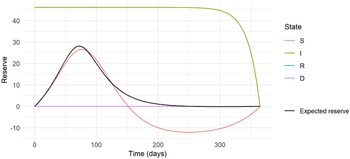


 Open access