1. Introduction
Satellite, Surface and Submarine observations have revealed a Significant areal reduction and thinning of arctic Sea-ice cover in the past 50 years (Reference VinnikovVinnikov and others, 1999). Satellite observations are mostly derived from passive-microwave Sensor measurements of total Sea-ice concentration (ct; See table 1 for a list of acronyms used in the text), available continuously Since 1978 (Reference Parkinson, Cavalieri, Gloersen, Zwally and ComisoParkinson and others, 1999). derived parameters Such as total Sea-ice-covered area and ice extent (total area with ct > 15%) Show a decrease of about 3%decade–1 for the northern hemisphere over this period (Reference Cavalieri, Gloersen, Parkinson, Comiso and ZwallyCavalieri and others, 1997; Reference JohannessenJohannessen and others, 2004). the exact cause of Sea-ice cover reduction is Still a matter of debate, as it could result from complex interactions between marine and atmospheric forcing and feedbacks (e.g. j. Reference Zhang, Rothrock and SteeleZhang and others, 2000). however, there is a growing recognition that anthropogenic climate warming Since the late 20th century may be partly responsible for the recent decline (Reference VinnikovVinnikov and others, 1999; Reference JohannessenJohannessen and others, 2004). Sea-ice response to natural and anthropogenic climate forcing may vary greatly between regions having different ice regimes (Reference Gloersen, Parkinson, Cavalieri, Comiso and ZwallyGloersen and others, 1999; Reference Parkinson, Cavalieri, Gloersen, Zwally and ComisoParkinson and others, 1999). for this reason, Studies of regional Sea-ice variability are needed in order to better understand Sea-ice dynamics and assess potential future changes.
Table 1. Definition of acronyms used in the text
The canadian arctic, defined here as including hudson bay (HB), the arctic archipelago and the davis Strait/labrador Sea (DS/LS) region, is made of an intricate network of channels, islands and bays with different and complex ice regimes (fig. 1). the projected retreat and possible disappearance of the Summer ice pack within this century (Reference VinnikovVinnikov and others, 1999) could open the way to increased marine Shipping via the northwest passage. however, it has been Suggested that a reduction of first-year ice formation could also allow for incursion of more older ice in the arctic archipelago, therefore complicating projections of future ice extent in that region (Reference Falkingham, Chagnon, McCourt, Frederking, Kubat and TimcoFalkingham and others, 2001; Reference Wilson, Falkingham, Melling and De AbreuWilson and others, 2004).

Fig. 1. Map of the Canadian Arctic Showing localities discussed in the text. HB: Hudson Bay; DS: Davis Strait; LS: Labrador Sea; NOW: North Open Water polynya; FB: Foxe Basin; HS: Hudson Strait. 1. Sverdrup and Peary Channels; 2. Norwegian Bay; 3. Parry Channel; 4. Cape Bathurst Polynya; 5. Coronation Gulf; 6. M’Clin-tock Channel; 7. Queen Maud Gulf; 8. Gulf of Boothia; 9. Committee Bay.
Here we present results of a Systematic investigation of recent (25 year) Sea-ice variability in the canadian arctic and related climatic control. for this analysis we use a gridded, high-resolution digital database of Sea-ice concentration for the period 1980–2004, recently produced by the canadian ice Service (CIS) at environment canada. this period was chosen because we are interested in the Seasonality of recent Sea-ice changes and ice charts only became available on a year-round basis after 1980.
2. Database and Methods
2.1. Sea-ice data
Observations of Sea-ice conditions have been collected by the cis Since 1968 as an aid to arctic Shipping, using a combination of Space- and airborne Sensors as well as Surface visual observations. these data were first published as regional weekly operational charts in the Shipping Season only (june–october). each chart is made of mapped polygons with Sea-ice ct and information on Sea-ice type. after 1980, winter charts were produced at 2–4 week intervals, and the accuracy of the database improved as the availability and precision of Sensors increased and the use of nowcasting techniques (interpolation of missing chart from past ice conditions and present meteorological conditions) decreased. detailed information on data acquisition, chart preparation procedures and chart accuracy is available in Reference Crocker and CarrièresCrocker and carrieres (2000). the weekly regional charts were recently digitized and merged into a Spatially and temporally consistent gridded database with a Spatial resolution of 0.25˚×0.25˚. thus pixel Size varies from 16km×27.8km at 55˚n to 4km×27.8km at 82˚ n. each weekly grid Supplies information on Sea-ice ct data in tenths per gridcell. the ct values are broadly consistent with those obtained from passive microwave Sensors, but the cis database offers a better coverage of transitional periods (freeze-up and break-up) than the microwave Sensors, which are biased due to difficulties in discriminating between melt ponds and open water (Reference Agnew and HowellAgnew and howell, 2003). for this Study, monthly ct averages were calculated over the period 1980–2004 by averaging the weekly ice-concentration data on a pixel-by-pixel basis. monthly averages include three to four weekly charts, except in winter (december–may) when one or two charts were used. if no weekly charts could be found at a particular gridpoint for a given month, this month was flagged as a missing value. the mean monthly climatology of Sea-ice ct was calculated by averaging the ct data at each gridpoint for the entire period of record (1980–2004). monthly ct anomalies were then computed by Subtracting the mean annual cycle from monthly averages. Seasonally averaged ct values were also calculated for the winter (january–march), Spring (april–june), Summer (july–september) and fall (october–december) gridded Series. Spatial linear trends in monthly ct anomalies and Seasonal ct values were determined by least-squares regression at each gridpoint.
The Spatio-temporal variability of monthly ct anomalies was investigated by the empirical orthogonal function (EOF) analysis method (Reference Ribera, Gimeno, Garcia, Hernandez, Venegas, Mateu and MontesRibera and others, 2001). briefly, the method ‘decomposes’ the total variance in the ct anomalies into a Set of mutually orthogonal eigenvalues and corresponding eigenvectors from the diagonalized covariance matrix of the ct anomalies. each eigenvector represents a Spatial pattern of ct anomalies whose evolution over time is obtained by projecting the eigenvector onto the original ct Series (the expansion coefficients). each Set of eigenvalue, eigenvector and expansion coefficient Series therefore defines a mode of Sea-ice variability which may be linked to a Set of natural processes (oceanic or atmospheric). in this Study, eigenvectors are represented by homogeneous correlation maps between the expansion coefficient Series and the original ct data matrix. Significance levels for correlations were determined at each gridpoint using the method of Reference SciremammanoSciremammano (1979). the method estimates the large lag Standard error:
Where Cxx and Cyy are the autocorrelation functions for variables X and Y, N is the Sample Size and Δt is the Sampling time interval. σ reflects the interplay between the dominant timescales of the process and the finite record length. for n degree of freedom (n=1/σ 2)>10, the 95% level for correlation corresponds to 2.0σ (Reference SciremammanoSciremammano, 1979). to reduce Sampling error at large lags (and Small Sample Size), we used biased estimates for Cxx and Cy y. this reduces the effect of longer fluctuations, which may be inadequately Sampled by Short Series. however, if the data length N is Smaller than the length of a Significant low-frequency component of X or Y, then σ (and hence confidence levels) may be underestimated. Sea ice typically has long-term (decadal) memory, especially near the ice edge. twenty-five years of data are Sufficient to Sample at least two decadal cycles and obtain reasonable estimates of σ, although increasing data length would increase the robustness of σ estimates. the field Significance (the minimum number of Significant correlations on a grid needed to be Significantly different than chance) was tested using the method of Reference Livezey and ChenLivezey and chen (1983). each gridded dataset was correlated 200 times with a gaussian white-noise Series, and the number of Significant correlations was recorded each time. the 95% percentile of the distribution was used as the objective criterion for field Significance. the minimum number of Significant correlations needed for correlation maps between EOFs and climatological fields (see Section 2.2) was around 1000 gridpoints, or 10% of the grid. unless Stated otherwise, all correlation maps were found to pass that threshold.
2.2. Climatological variables
Monthly averages of Sea-level pressure (SLP) and Surface air temperature (sat) from the us national centers for environmental prediction (NCEP) re-analysis data (Reference KalnayKalnay and others, 1996) were obtained through the us national oceanic and atmospheric administration (noaa) cooperative institute for research in environmental Sciences (CIRES) climate diagnostic center. we used monthly Sea-surface temperature (sst) averages from the extended reconstructed Sst database (ERSST v.2; Reference Smith and ReynoldsSmith and reynolds, 2004), obtained through the national climatic data center at noaa. the SLP and Sat data have resolutions of 2.5˚×2.5˚, and the Sst data have a resolution of 2˚×2˚. mean monthly wind vector components (u,v) were calculated from the monthly SLP data as Surface geostrophic wind. geostrophic winds were preferred to Surface winds from ncep because they are less model-dependent (Reference KalnayKalnay and others, 1996) and because, as a rule, Sea-ice drifts follow geostrophic winds on Subannual timescales (Reference Thorndike and ColonyThorndike and colony, 1982). monthly anomalies of SLP, Sat, Sst, u- and v-wind components were calculated in the Same way as for the ct data.
The relationships between climatic variables and the principal modes of Sea-ice ct variability were investigated through the use of heterogeneous correlation maps, defined as the vector of correlation values between the expansion coefficient of a particular ct EOF mode, and all Successive gridpoint values of a given climatic field (sat, SLP, Sst, u and v-wind). correlation maps were prepared at different leads and lags (typically ±12 months) to explore potential forcing and feedback mechanisms between Sea-ice and climatic variables. in addition, we used monthly indices of the main atmospheric teleconnection patterns in the northern hemisphere (Reference Barnston and LivezeyBarnston and livezey, 1987) obtained from the climate prediction center at noaa to investigate potential relationships between Sea-ice variability and hemispheric modes of atmospheric circulation.
3. Results and Discussion
3.1. Sea-ice climatology and trends, 1980–2004
figure 2 illustrates the mean Seasonal climatology of Sea-ice ct in the canadian arctic for the period 1980–2004. maximum ice extent occurs in february, with the eastern edge of the ice pack located in the DS/LS region. ice break-up begins in april–may in hb, the beaufort Sea and the north open water polynya (now) in north baffin bay, while the ice edge in the ls begins to retreat northward. minimum ice extent is reached in late Summer to early fall (august–september), with the ice edge located north of eastern parry channel. heavy ice concentrations (>80%) remain west of parry channel, in m’clintock channel, committee bay and in nares Strait. baffin bay is mostly ice-free in Summer, but light ice (<35%) may remain off the eastern coast of baffin island. ice freeze-up begins in early october in the canadian arctic archipelago, northern foxe basin, baffin bay and the northwestern part of hb. the remaining Southern areas become encumbered with ice moving with ocean currents and weather Systems (CIS, 2002).

Fig. 2. Maps of Seasonal CT averages, 1980–2004: (a) winter; (b) Spring; (c) Summer; and (d) fall.
Maps of Seasonal ct Standard deviations are presented in figure 3. high (low) Standard deviations indicate large (small) year-to-year variability in Sea-ice ct. the most pronounced variability occurs in winter in the DS/LS region and in Summer in the beaufort Sea. other areas of Significant variability include the coastal regions of north baffin bay in Spring–summer, and the northwestern and Southeastern coasts of hb as well as the DS/LS region in the Spring.

Fig. 3. Maps of Seasonal CT Standard deviation, 1980–2004: (a) winter; (b) Spring; (c) Summer; and (d) fall. ct in the DS/LS region (Reference Gloersen, Parkinson, Cavalieri, Comiso and ZwallyGloersen and others, 1999), whereas our analysis Shows a Substantial reduction in this area.
Linear trends in monthly ct anomalies for 1980–2004 (fig. 4a) reveal maximum ice-cover reductions (>˚% decade–1) in the beaufort Sea, DS/LS region, hudson Strait/ungava bay and along the coast of Southern baffin island. important reductions also occur in northwestern hb and Southern foxe basin (4–˚% decade–1), while Smaller but Statistically Significant reductions occur in foxe basin, coronation gulf, queen maud gulf and the gulf of boothia (2–4% decade–1). a marked increase in ct occurs off the western coast of banks island, in the region of the cape bathurst polynya, while local increases are noted in Smith Sound, in wellington channel and in the norwegian bay area. the normalized total Sea-ice area (NTA; fig. 4b) for the whole canadian arctic Shows an overall reduction of 3.6% decade–1, consistent with previous findings (Reference Gloersen, Parkinson, Cavalieri, Comiso and ZwallyGloersen and others, 1999; Reference Parkinson, Cavalieri, Gloersen, Zwally and ComisoParkinson and others, 1999). however, previous trends calculated from Satellite passive microwave Sensor data for the period 1978–96 Showed an increase in

Fig. 4. (a) Map of linear trends in CT monthly anomalies, 1980–2004. Inset Shows areas with Statistically Significant trends (p < 0.05). (b) Normalized total ice area (NTA) and corresponding least-squares linear trend for the whole Canadian Arctic, 1980–2004. NTA is calculated by dividing the total ice area by the area covered by all available gridpoints. This minimizes the influence of any missing gridpoint on the calculated ice area.
On a Seasonal basis, the negative ct trends occur predominantly in Spring and Summer (fig. 5). maximum reduction occurs in the beaufort Sea in Summer (14 to >24% decade–1). the decrease in the DS/LS region occurs mainly in winter and Spring, with rates over 18%decade–1, while the decrease in northwestern hb is mainly in the Spring (>12% decade–1), and in Summer to a lesser extent. apart from the negative trend in the DS/LS region (not Statistically Significant), very little change is observed during the winter. maximum reduction rates during Spring and Summer are consistent with earlier findings (Reference Parkinson, Cavalieri, Gloersen, Zwally and ComisoParkinson and others, 1999; Reference Walsh and ChapmanWalsh and chapman, 2001; Reference JohannessenJohannessen and others, 2004). although arctic multi-year (older) ice cover has been decreasing more rapidly (7–9% decade–1) than the total ice cover in the last 20–22 years (Reference ComisoComiso, 2002), our analysis Shows little decrease in ice cover in the queen elizabeth islands (QEI), an area covered year-round predominantly by multi-year ice (CIS, 2002). this confirms results by t. agnew and others (unpublished information) and Reference Jeffers, Agnew, Alt, De Abreu and McCourtJeffers and others (2001) who found no Statistically Significant trends in the maximum amount of Summer open water in the qei for the period 1961–98.

Fig. 5. Maps of Seasonal linear trends in CT: (a) winter; (b) Spring; (c) Summer; and (d) fall. Insets Show areas of Statistical Significance (p < 0.05).
3.2. Spatio-temporal variability of Sea-ice cover
The four leading EOF modes of Sea-ice ct were verified to be uncorrelated according to north’s rule of thumb (Reference North, Bell and CahalanNorth and others, 1982), and together these modes explain 32% of the total variance in monthly ct anomalies. individually, they explain 12.3%, 9%, 6% and 4.6%, respectively. the first EOF mode (EOF1) identifies a broad area of coherent Sea-ice cover variability that encompasses hb and the DS/LS region (fig. 6). this mode explains up to 25% and 50% of Sea-ice variance in these two regions, respectively (local variance explained = Square of the correlation value). in contrast, EOF2 identifies a dipole pattern of opposition between hb and the DS/LS region, explaining up to 45% and 20% of local Sea-ice variance, respectively. a Secondary positive centre of action is also found in the beaufort Sea, explaining about 8% of local variance. EOF3 displays an antiphase pattern between the beaufort Sea (up to 65% variance explained) and baffin bay (up to 29% variance explained). the northwestern part of hb also loads positively in EOF3, but with only 5% of local variance explained. EOF4 Shows opposite centres of action in the northern and Southern parts of HB, with 25% and 20% of local variance explained, respectively. weaker negative correlations occur along a narrow band extending South from davis Strait along the labrador coast, while positive correlations are found offshore in the labrador Sea.

Fig. 6. Homogeneous correlation maps for the first four EOF modes. Only Statistically Significant correlations (p < 0.05) are Shown.
Over time, EOF1 Shows both low-frequency (decadal) variability and interannual variability, while EOF2, EOF3 and EOF4 mainly display interannual variability (fig. 7). Spectral analysis revealed that EOF1 has Strongest power at ∽10 year period, with a Smaller peak at ∽1 year. the temporal variance of EOF2 is Spread over a broader Spectrum of frequencies but Shows maximum power at ∽1 year. EOF3 and EOF4 both have maximum Spectral power around ∽2.7 years, with Smaller peaks at <1 year. the Seasonality of each EOF mode was investigated by computing the monthly Standard deviation of each expansion coefficient Series (fig. 8). EOF1 is mainly a cold-season pattern (november–june). EOF2 has maximum variability in the transition periods (freeze-up in november and melt in june–july). EOF3 is mainly a Summer to early-fall pattern (june–october) and EOF4 is mainly an early- to mid-summer pattern (may–july).

Fig. 7. Standardized expansion coefficient Series for the first four EOF modes. The thick lines represent a 13-point (0.5,1. . .1,0.5) running mean to highlight interannual variability.

Fig. 8. Monthly Standard deviation for the first four EOF modes.
The variance recovered by the four leading EOF modes is Similar to that found from hemispheric Sea-ice databases (Reference Singarayer and BamberSingarayer and bamber, 2003). this rather low value implies (1) that there may be other Significant modes of variability which are unresolved by our analysis due to the Short period of record and/or (2) that a Significant portion of the total variance represents noise. in particular, the inter-channel areas of the qei are underrepresented in the first four EOFs. this Suggests that Sea-ice variability in the qei is localized and Shows little connection with the broader areas of open ocean. also because the channels are ‘under-sampled’ compared to the broader areas of open ocean, their variance is not likely to be captured by the dominant EOFs.
3.3. Sea-ice–climate relationships
3.3.1. EOF1
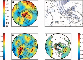
Heterogeneous correlation maps between the expansion coefficient Series of EOF1 and climatological field anomalies (SLP, Sst, Sat, winds) are presented in figure 9. on these maps, large positive (negative) correlation indices denote Strong positive (negative) correlations between EOF1 and normalized anomalies of the climatological fields (e.g. SLP). the correlation pattern for SLP anomalies (fig. 9a) Shows a Strong opposition between the greenland Sea and a latitudinal band Stretching along the 40˚n parallel from newfoundland to western europe. Strongest correlation values occur over newfoundland (0.32) and the denmark Strait (–0.39), which is the normal position of the icelandic low. this dipole pattern of SLP anomalies resembles the positive phase of the arctic oscillation (AO; Reference Thompson and WallaceThompson and wallace, 1998), and even more closely the north atlantic oscillation (NAO; Reference HurrellHurrell, 1995). this was confirmed by correlating the winter (december–february) portions of the EOF1 and nao index Series, which gave r = 0.54 at lag 0. a weaker but Significant negative correlation was also found between EOF1 and the el niño–southern oscillation (ENSO) monthly SLP index at lag +3 months (i.e. ENSO leading by 3 months). these results are consistent with observations by Reference Wang, Mysak and IngramWang and others (1994) and Reference Mysak, Ingram, Wang and van der BaarenMysak and others (1996), who found positive Sea-ice anomalies in hb and the labrador Sea when Strong episodes of ENSO occurred in the previous Summer and during positive phases of the nao during winter of the Same year.
Fig. 9. Heterogeneous correlation maps (lag 0) between EOF1 and monthly anomalies of (a) SLP; (b) u- and v-wind components; (c) SAT; and (d) SST. Color bars and arrow length represent the Strength of the correlation coefficient. Black contours delineate areas of Statistical Significance (p < 0.05). indices (fig. 13a) revealed a Statistically Significant relationship with pna at lag 0 (r = 0.16), with ENSO at lag +4 months (r = 0.22) and with the nino3 index at lag +5 months (r = 0.34). the better correlation with the nino3 and ENSO indices indicates that the link between EOF3 and the pna is mostly due to ENSO fluctuations. the variability of EOF3 over time is dominated by a few high-amplitude events, which are often preceded by an ENSO event (fig. 13b). the cross-correlation function with ENSO and nino3 Suggests an oscillation with a period of ∽2–4 years, consistent with the timescale of ENSO variations (2–6 years) and with the low-frequency part of EOF3.
Fig. 10. Same as Figure 9 but for EOF2.
Fig. 11. Same as Figure 9 but for EOF3.

Fig. 12. Same as Figure 9 but for EOF4.

Fig. 13. (a) Cross-correlation plot between EOF3 expansion coefficients and monthly indices values of the PNA, ENSO and Nino3 indices. Note: El Niño events are defined by a negative ENSO index and positive Nino3 index, while the PNA tends to be inversely correlated with ENSO. (b) Plot of EOF3 expansion coefficients (black curve) and Nino3 index (grey curve). Black dots represent NAO events below one Standard deviation of the monthly NAO index (only the maximum monthly value within the extreme year is Shown).
Changes in the Strength and distribution of SLP anomalies may affect Sea ice through dynamic (wind) and thermodynamic (air-temperature) forcing. the correlation map of EOF1 with wind anomalies (fig. 9b) Shows that an anomalous cyclonic circulation over greenland combined with anticyclonic circulation over newfoundland induces Strong northwesterly wind anomalies in the outermost part of the DS/LS region (fig. 9b), favouring a Southward advection of ice in winter and Spring. the northwesterly wind anomalies also cause advection of cold arctic air into the eastern canadian arctic, hb and labrador Sea, promoting the growth and preservation of positive Sea-ice anomalies in these areas (fig. 9c). the correlation pattern for Sat (fig. 9c) is consistent with the Spatial Signature of a positive nao, with cold and dry winters in northern canada and greenland (Reference HurrellHurrell, 1995). EOF1 also Shows Strong negative correlations with Sst over the north atlantic region (fig. 9d). lag correlation maps between EOF1 and Sst (not Shown) Show negative Sst anomalies appearing in Southwestern greenland 1 year before the positive ct anomaly develops in the DS/LS and hb regions. the Sst anomaly progressively expands eastward into the norwegian Sea up to 6 months after the ct anomaly, and Southward toward the newfoundland coast where it dissipates 1–1.5 years after the ct anomaly. the lag-correlation maps between EOF1 and Sat also Show Strong negative Sat anomalies developing 1 year before EOF1 but decaying a few months later (not Shown). this is in good agreement with recent results Showing that decadal cold climatic episodes and positive ice-cover anomalies around greenland and baffin are accompanied by cold Sst anomalies lasting 1–3 years after the decay of ice-cover anomalies (Reference Rogers, Wang and McHughRogers and others, 1998; Reference Deser, Holland, Reverdin and TimlinDeser and others, 2002).
When normalizing the correlation coefficients by their estimated large-lag Standard errors, Sat (σ max = 5.2σ) appears most Strongly related to EOF1, followed by SLP and winds (σ max ∽ 4.6σ) and Sst (σ max = 3.8σ). these results Suggest that atmospheric temperatures contribute more to the ct anomalies expressed by EOF1 than dynamic forcing. these conclusions complement recent results by Reference Prinsenberg, Peterson, Narayannan and UmohPrinsenberg and others (1997) and Reference Deser, Holland, Reverdin and TimlinDeser and others (2002) who found that positive anomalies develop in the DS/LS region in response to anomalous northwesterly winds within the labrador Sea and offshore flow east of newfoundland. a Subsequent model Simulation by Reference Deser, Holland, Reverdin and TimlinDeser and others (2002) Suggested, as reported here, a dominance of thermodynamic processes over dynamic mechanisms.
3.3.2. EOF2
Significant but weaker correlations occur between EOF2 and SLP anomalies, with maximum negative polarity over the labrador Sea (r = –0.21) and maximum positive polarity (r = 0.17) over western and Southern north america (fig. 10a). lag-correlation maps (not Shown) Suggest that negative SLP anomalies lead positive EOF2 anomalies by 1–2 months in the DS/LS region, while the Smaller positive SLP anomaly appears farther South 2 months earlier. the associated wind pattern Shows northerly wind anomalies over much of the eastern canadian arctic, and Southeasterly and easterly wind anomalies over davis Strait (fig. 10b). correlation with Sat Shows maximum values over the DS/LS region (r = 0.42) and minimum values (r = –0.25) over eastern canada/USA (fig. 10c). positive Sat anomalies lead the positive EOF2 anomalies by 3–4 months, gradually expanding over the DS/LS region and dissipating 1 month after the ct anomaly, while negative Sat anomalies only appear at lag 0 and dissipate 1 month after the ct anomaly (not Shown). closer inspection of the expansion coefficient Series of both EOF1 and EOF2 (fig. 7) reveals that although both Series are Statistically uncorrelated as a whole, EOF2 includes much of the annual to Sub-annual variability of EOF1. their winter Structure is Similar, being inversely correlated at r = –0.99. the winter portion of EOF2 is in turn also correlated with the winter NAO, but negatively (r = –0.55). So while EOF1 represents a predominately decadal Signal most active during the cold Season, EOF2 appears to be an annual to Sub-annual expression of this first mode, which is related to the winter NAO. it is thought that the dipole between the DS/LS region and HB, which is Superimposed on EOF1, results from local ice-to-atmosphere feedbacks controlled by the coupled interannual variability of the NAO and ice cover in the DS/LS region. reduced ice cover in the DS/LS region during a more negative NAO allows for turbulent heat transfer from the ocean to the atmosphere, causing local warming and decreased SLP (fig. 10a and c). the fact that the Sat anomalies associated with EOF2 appear 1–2 months before the SLP anomaly Supports this idea. the local SLP anomaly induces northerly winds and advection of cold air over part of HB, promoting positive ice anomalies in that region. the reverse process occurs when ice cover increases during winter in the DS/LS region in response to a more positive NAO. this hypothesis is Supported by recent results Showing high upward turbulent heat-flux anomalies occurring in the DS/LS region when negative ct anomalies occur in winter (Reference Deser, Walsh and TimlinDeser and others, 2000, Reference Deser, Holland, Reverdin and Timlin2002). when taking the Standard errors of correlation into account, the onshore Surface winds and positive temperature anomalies in the DS/LS are the most Significant feature associated with EOF2 (r >4σ). the Sst pattern of figure 10d, which is only present at lag 0, may represent a direct effect of ct variability associated with EOF2: decreased (increased) Ssts occur in areas of increased (decreased) Sea-ice cover. alternatively, the correlation may reflect the effect of the parameterization between Sst and Sea-ice concentration in the ERSST database (Reference Smith and ReynoldsSmith and reynolds, 2004).
3.3.3. EOF3
Slp anomalies associated with EOF3 Show a weak dipole with positive polarity over the arctic ocean (r = 0.20) and negative polarity over the bering Sea (r = –0.15) (fig. 11a). the positive SLP anomaly developed 3–4 months earlier over the arctic ocean, while the negative anomaly over the bering Sea appeared 1 month earlier (not Shown). the Surface wind pattern associated with EOF3 Shows anomalous offshore winds along the beaufort Sea coast and anomalous northerly and Southerly winds over nares Strait and baffin island, respectively (fig. 11b). correlation with Sat Shows a warming over northwestern north america and cooling over the north pacific and northwestern USA (fig. 11c). the Sst pattern Shows warming in the beaufort Sea (fig. 11d), which began 3–4 months before the ct anomaly and disappeared 2 months later (not Shown). when normalizing the correlation by their Standard error, Sst appears as the dominant factor (r = 6σ), followed by wind and Sat (r = 3.6σ), and SLP (r = 3.3σ).
The positive ctanomaly in baffin bay Seems to be a direct result of the anomalous anticyclonic circulation over the arctic ocean, which promotes advection of ice into baffin bay through nares Strait (fig. 11b). at the Same time, the anomalous Southerly winds over baffin island may restrain the ice from moving South, thereby maintaining the positive ct anomaly. the most prominent feature of EOF3, however, is the negative ct anomaly off the beaufort Sea coast (see fig. 6c). the anticyclonic SLP anomaly over the arctic appears to be causing most of the dynamical forcing on Sea ice, by inducing offshore wind anomalies which promote export of ice from the beaufort Sea toward the eastern arctic (fig. 11b). on the other hand, the cyclonic anomaly over the bering Sea acts as a thermodynamic forcing on Sea ice by driving warm pacific air into the beaufort Sea and western coast of north america (fig. 12b and c). the position of the two centres of SLP variability is typical of late-spring to early-summer conditions, when the beaufort high and the aleutian low begin to dissipate. because the Sstanomalies are locally restrained to the beaufort Sea region, they are more likely to act as a positive feedback on Sat and ice cover rather than being the main driver of the ct anomalies. it is likely that preconditioning of the ice pack during Spring by enhanced offshore wind and positive temperature anomalies triggered the decrease in ct, with positive Ssts developing Simultaneously and further enhancing the decrease in ct through thermodynamic effects.
The SLP and Sat patterns of figure 11 have Similarities with the pacific/north american teleconnection pattern (pna; Reference Barnston and LivezeyBarnston and livezey, 1987). the PNA is one of the most prominent modes of low-frequency variability in the northern hemisphere. its positive phase is associated with above-average SLP in the vicinity of hawaii and over the inter-mountain region of north america, and below-average SLP over the aleutian islands and over the Southeastern united States. increased (decreased) Sat occurs over northwestern north america and the north pacific, respectively. although the pna is a natural internal mode of climate variability, it is Strongly affected by ENSO, with positive phases of the pna being associated with ENSO years (Reference Stocker and HoughtonStocker and others, 2001, p. 453). cross-correlation between EOF3 and the pna, ENSO (SLP) and nino3 (sst)
The positive SLP anomaly over the arctic differs from the pna pattern and Suggests an influence from the north atlantic (fig. 11a). a weak but Statistically Significant negative correlation was found between EOF3 and the monthly nao index at lag +1 month (r = –0.16). however, the largest anomalies in EOF3 occur when nao and ENSO events occur Simultaneously (fig. 13b). the most Striking example is the extreme year of 1998 during which the largest ENSO event over the Study period occurred in combination with the Second largest nao event. the amplitude of the ct anomaly appears to depend on the Synchronicity of both indices. a weakening of the beaufort gyre occurs during winter/spring under a negative nao regime, which tends to increase ice export from the beaufort Sea (Reference KwokKwok, 2000). thus large negative ct anomalies in the beaufort Sea result from preconditioning of the ice pack during winter–spring combined with the thermodynamic and dynamic forcing induced by ENSO events. these results complement recent findings by Reference Maslanik, Serreze and AgnewMaslanik and others (1999) who found Similar SLP anomaly patterns from composite charts associated with light ice years in the beaufort Sea. they Suggested that both the nao and ENSO could have an impact on ice anomalies in the area but found no clear relationships. the present application of the EOF method allowed for the extraction of the variance in the beaufort Sea region associated with these two modes of climate variability.
3.3.4. ;EOF4
The SLP pattern associated with EOF4 (fig. 12a) Shows a weak positive anomaly over central canada (r = 0.16) resulting in anomalous northwesterly winds over hb, while anomalous Southerly winds occur along the eastern coast of baffin island in response to a weak decrease in SLP over Southern baffin island (fig. 12b). Similar Sat and Sst patterns are found, with increased temperature over the western coast of north america and bering Sea and reduced temperature over the central north pacific (fig. 12c and d). decreased Sat also occurs over Southern hb (fig. 12c). the Strongest correlations between EOF4 and Sst occur within hb (r = 0.46), but Since these only appear at lag 0, they most likely reflect the effect of the parameterization between Sst and Sea-ice concentration in the ersst database (Reference Smith and ReynoldsSmith and reynolds, 2004).
The Spatial patterns of SLP, Sat and Sst are Strongly apparent to the east pacific–north pacific teleconnection index (ep-np; Reference Barnston and LivezeyBarnston and livezey, 1987). the ep-np is a Spring–summer–fall pattern whose positive phase is associated with a Southward Shift and intensification of the pacific jet Stream from eastern asia to the eastern north pacific, followed downstream by enhanced anticyclonic circulation over western north america and by enhanced cyclonic circulation over the eastern united States. the positive phase of the EP-NP pattern is associated with above-average Surface temperatures over the eastern north pacific, and below-average temperatures over the central north pacific and eastern north america. maximum correlation between EOF4 and the monthly EP-NP (r = 0.21) occurs when the EP-NP leads EOF4 by 1 month. on a Seasonal basis, Significant correlations were found between EOF4 and the EP-NP during Spring (r = 0.63) and Summer (r = 0.57), in accordance with the Seasonality of both EOF4 and the EP-NP. when Scaling all correlations by their Standard errors and ignoring the correlation between EOF4 and Sst in hb, Sst and Sat appear to have a Stronger influence on EOF4 (r=3σ) than does SLP and winds (r=2.5σ). EOF4 thus appears to result from Springtime climate variability in the north pacific region, which induces anomalous anticyclonic circulation over central/ western north america. the resulting Southward advection of cold arctic air over hb retards ice melt in the Spring while the northwesterly winds tend to push the ct anomalies toward the Southern portion of hb. the weaker dipole in the DS/LS region may result from the opposition between the Southerly winds anomalies along the eastern coast of baffin island and the northwesterly wind anomalies over labrador.
4. SUmmary and Conclusions
The analysis of the new cis digital Sea-ice database has allowed a thorough and detailed assessment of recent Sea-ice variability in the canadian arctic. the results of our EOF analysis applied on monthly ct anomalies have Shown that the principal modes of Sea-ice variability in the canadian arctic have Seasonal dependency as well as connections with preferred modes of atmospheric and Sst variability. one recurrent aspect of this Study is the preponderant influence of the nao on Sea-ice variability during the cold Season. the dominant mode of Sea-ice variability in the canadian arctic is a north–south contraction of the ice edge in the DS/LS region (and hb to a lesser extent) during the cold Season, which oscillates on a decadal timescale in response to the nao. this mode most probably reflects the broader, hemispheric-scale Seesaw in ice extent between the greenland Sea and the DS/LS region identified in previous Studies (Reference Yi, Mysak and VenegasYi and others, 1999; deser and others, 2000; Reference Partington, Flynn, Lamb, Bertoia and DedrickPartington and others, 2002) and which occurs in response to decadal variations in the AO/NAO. the Seesaw between hb and the DS/LS region captured by EOF2 may represent a more local mode of variability in which interannual changes in ice extent in the DS/LS region, possibly driven by the high-frequency variations of the nao (e.g. Reference MarshallMarshall and others, 2001), Succinctly impact on hb via ice-to-atmosphere feedbacks.
Sea-ice variability during the warm Season, captured by EOF3 and EOF4, Showed connections with climate variability in the pacific ocean as well as in the atlantic Sector. the Sensitivity of the beaufort Sea to both pacific and atlantic climate variability means that the ice regime may be punctuated by extreme years of negative and positive ice anomaly, as was the case in 1998. the ice regime of the geographically bound hb is more Sensitive to Springtime climate variability and So was found to respond to the Strength and position of the pacific jet Stream, as measured by the EP-NP index.
Of the four dominant modes of Sea-ice variability in the canadian arctic, only EOF1 displays a Significant negative trend. however, the trend is not a monotonic decrease, being influenced by the low-frequency variability of EOF1. this low-frequency component also dominates the total ice-area variability (fig. 4b). the large negative trends found in the DS/LS region during winter are not Statistically Significant and result from this low-frequency variability, with Sea ice declining Since the mid-1990s in response to a decrease in the nao index. little or no warming trend has been reported for the eastern canadian arctic that could explain the decrease in ct also occurring in that area in the Spring, and it is likely that much of the decline also reflects the recent decrease in the nao index. on the other hand, the Strong negative trend found in the beaufort Sea occurs in accordance with regional and hemispheric Sat trends, which Show greatest warming during Spring and Summer over the western canadian arctic over the past 25 years (x. Reference Zhang, Vincent, Hogg and NiitsooZhang and others, 2000; Reference JohannessenJohannessen and others, 2004). the beaufort Sea, like the other peripheral Seas of the arctic (chukchi, east Siberian, laptev and kara Seas), appears most Sensitive to the recent climate warming, displaying a consistent decline in ice cover over the past 25 years. conversely, the canadian arctic archipelago Shows the least change over the past 25 years. it is then possible that this region, with its more complex physiographic and climatic conditions, will experience a Slower ice retreat than that predicted for the rest of the arctic over the next century.
This Study has Shown that in the canadian arctic (hb, DS/LS and the canadian arctic archipelago) interannual to decadal variability predominates over long-term trends. moreover, linear trends calculated over periods of 20–30 years may be highly influenced by low-frequency components of Sea-ice variability. extrapolation of trends in areas where Such low-frequency variability prevails is thus unlikely to give reliable estimates of future ice conditions. this highlights the need for longer Series of Sea-ice variability, in order to isolate any trends due to anthropogenic global warming from the decadal Sea-ice variability present in many regions. in this regard, proxy-based reconstruction of past Sea-ice variability may help to reach these objectives (Reference Kinnard, Zdanowicz, Fisher and WakeKinnard and others, 2006).
Acknowledgements
This Study was funded by the cryosphere System in canada project (CRYSYS) at environment canada, and the canadian foundation for climate and atmospheric Sciences (Cfcas). funding to c. kinnard by the natural Sciences and engineering research council of canada (NSERC) is also appreciated. we thank a. tivy for help in accessing the cis database.