


Introduction and Survey
For about one hundred years, scientists have been engaged in determining the changes of the surface of glaciers. In the special case of the Vernagtferner, accurate topographic maps have been available since 1889 and were used for the calculation of changes in volume and elevation of the glacier (Reference Brunner and RentschBrunner and Rentsch 1972). These changes of the surface of glaciers were deduced from contour plots of different years. The contours had to be digitized, using planimeters in most cases. As already mentioned in Reference Peipe, Reiss and RentschPeipe and others (1978), the data processing for this method is rather complicated and inconvenient. In this paper, the use of Digital Elevation Models (DEM), or equivalent Digital Terrain Models (DTM), for the determination of changes in volume and elevation of the glacier, will be introduced. First, the generation of a DEM and the determination of changes in volume and elevation from the DEM are described. Next, the contour method is briefly described and a comparison between both methods is carried out on part of the Vernagtferner, for the years 1979 and 1982, The changes in volume and elevation for the whole glacier area, deduced from the DEMs, are presented and the paper concludes with comments on the results.
Generation of Digital Elevation Models
The Digital Elevation Model is a description of a surface (especially the terrain surface), by digital means. So-called regular DEMs have some advantages concerning data processing and storage and were used here, too. The meshes of a regular DEM form a square grid in plane. The elevations of the grid points can be measured directly in the stereo mode, or interpolated from arbitrarily-distributed reference points.
Data acquisition
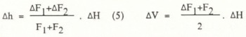
Density and distribution of the measured reference points determine the quality of the final DEM substantial. A survey of techniques of photogrammetric data acquisition is given in Reference Ebner and EderEbner and Eder (1984), For the data acquisition of the DEMs, we used Vernagtferner registrated contour lines in 1979 and the method of Progressive Sampling in 1982.
For the year 1979, the task consisted of direct contour plotting, on the one hand, and the determination of the controlling profiles for an analytical orthoprojector, on the other (Reference RentschRentsch 1982). For this reason, contour plotting was done with the analytical plotter, Zeiss Planicomp C 100. Simultaneously, the intersections of the contour lines with a regular grid were recorded. Additionally, break lines were measured.
For the year 1982, the program PROSA (Reference Ebner and ReinhardtReinhardt 1984) was used for data acquisition. This program runs in conjunction with the analytical plotters, Zeiss Planicomp, and is based on the method of Progressive Sampling. Data acquisition starts with the measurement of break lines and a sparse grid, which subsequently is densified, according to the local shape of the terrain and the accuracy requirement.
DEM Interpolation
For DEM Interpolation, various algorithms and computer programs are available (e.g. Reference KrausKraus 1984). The DEMs of the Vernagtferner were interpolated with the mini-computer program, HIFI (Height Interpolation by Finite Elements) (Reference Ebner, Hofmann-Wellenhof, Reiss and SteidlerEbner and others 1980), of the Chair of Photogrammetry TU Munich. HIFI interpolates the elevations of grid points from the elevations of arbitrarily-distributed reference points and points along break lines. More details concerning DEM data acquisition and interpolation using PROSA and HIFI are given in Reference Ebner and EderEbner and Reinhardt (1984).
All computational work concerning DEMs in this paper, such as interpolation of DEMs, derivation of contours and volumes was done with the HIFI program system mentioned above.
Determination of Changes in Volume and Elevation from Digital Elevation Models
Calculation of volume
For the calculation of volume, using a regular DEM the volumes of quadratic pillars have to be summed up! e quadratic pillars are limited by a horizontal square on the bottom and a hyperbolic paraboloid on the top (see Fig.1).
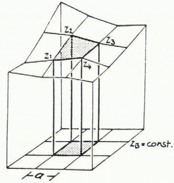
Fig. 1
The volume of one of these quadratic pillars can be calculated from equation (1) (Reference KrausKraus 1984).
with fq = a2, a = grid width
The whole volume within the rectangular DEM area can then be caluclated from:
with:
-
ZB — the elevation of the horizontal plane ZB=const
-
Zci — the elevations of the four corner points of the DEM
-
ZMi — the elevations of the nl = 2nx+2ny-8 other margin point of the DEM
-
ZIi — the elevations of the n2 = (nx-2)(ny-2)other points of the DEM
-
nx — the number of points in x-direction of the DEM
-
ny — the number of points in y-direction of the DEM
Changes in volume
To determine changes in volume, two DEMs, from two different epochs, have to be available. These DEMs have to cover the same area and must have identical grids in plane. In glacier research, it is usual to specify changes in volume for 100 m intervals. Therefore, the volume of each DEM, defined by two horizontal planes with a difference in elevation of 100 m, has to be computed. These volumes are ontained from equation (2) by setting ZB on a level with these horizontal planes subsequently for both years. The difference in volume corresponding to the epochs T1 and T2 and the horizontal planes Zi and Zi+1 (see Fig.2) is then given by:
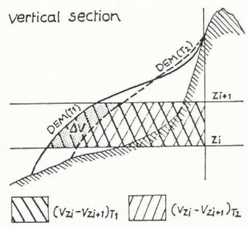
Fig. 2
Changes in elevation
The change in elevation of different epochs will be defined as the mean value of the differences in elevation, Δhi, of the n DEM points:
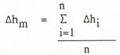
To calculate this mean value with respect to the 100 m intervals, the differences, Δhi, for each 100 m interval have to be summed up and their number has to be counted. With these specific values, the mean value of a 100 m interval can be calculated from equation (4).
Practical aspects
From a theoretical point of view, it is sufficient to establish two DEMs of different epochs, which are covering the same area and have grid points with identical coordinates in plane, and use them for the calculation of changes in volume and elevation. But, in practice, the data acquisition of the different DEMs can be systematically affected by different orientations and/or operators. To make sure that uncontrolled systematic errors are avoided, in practice, it is useful to transform the measured terrain coordinates of one epoch on to the terrain coordinates of the other epoch. For this purpose, in both cases, identical points have to be measured. This kind of point can be found at the surrounding rock areas of the glacier. For a final test, it is recommendable to derive contours from the DEMs after this transformation and to compare these contours in the surrounding areas.
In general, the regular grid DEM of the glacier also covers areas where no change in elevation should occur. To ensure that effects from random errors of the measurement in these areas do not interfere with the calculation of the changes in volume and elevation within the surface of the glacier, it is best to avoid calculations in there. For this reason, the outlines of the glacier surface have to be recorded İn the stereo model.
Determination of Changes in Volume and Elevation, using the Contour Method
This method should be briefly introduced here, because it is compared later with the method introduced above. For the determination of changes in volume and elevation, contour plots of two different epochs are required. The contour plots have to coincide in areas beyond the glacier surface.
Figure 3 shows contours from two different epochs, T1 and T2. The areas FI, F2, ΔF1, ΔF2 have to be determined planimetrically. From these values and the contour interval, ΔΗ, the desired changes of the glacier can be calculated from equations (5 and 6) (for details see Reference FinsterwalderR. Finsterwalder 1953).
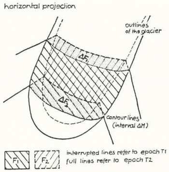
Fig. 3
Comparison of the two Methods on Part of the Vernagtferner
To compare the different methods introduced in sections 3 and 4, with respect to economy and accuracy, both methods were applied to determine changes in volume and elevation on part of the Vernagtferner. Because planimetrie work requires a lot of time, the area was limited to 2500 x 1140 m2
All the measurements necessary for this paper were obtained from the following material:
-
seven stereo models covering the Vernagtferner area; images taken on 14. 08. 1979, focal length 153 mm, image scale ~ 1:20 000
-
two stereo models covering the Vernagtferner area; images taken on 14. 09. 1982, focal length 153 mm, image scale ~ 1:33 000
For these investigations, first, a dense 20 m square DEM (7308 points) was measured directly for both epochs, using an Analytical Plotter, Zeiss Planicomp. Next, for 1979, a direct contour plot was drawn and digital contours were derived from the 20 m DEM. As also shown in Reference RentschRentsch (1982), the direct contour plot and the digital contours were identical on the glacier surface. For that reason, digital contours derived from both 20 m DEMs were used for the determination of changes of the glacier by the contour method. Thus, the comparison now is performed with the same data sets, in order to avoid an influence of different measurements with different random errors. Additionally, the outlines of the glacier surface were recorded.
Figure 4 shows the digital contours derived from 20 m DEMs of 1979 and 1982. The measured data of 1982 were transformed by identical points on to the system of 1979, as described above.
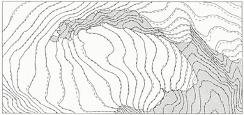
Fig. 4 20 m contours derived from the 20 m DEMs 1979 (continuous line) and 1982 (interrupted line) and outlines of the glacier for a sub-area of the Vernagtferner.
Now the changes in volume and elevation on this part of the glacier were derived from:
-
a 20 m and a 40 m DEM, where the 40 m DEM was obtained from the 20 m DEM
-
contours with 10 m, 20 m and 50 m contour interval
For the comparison of the different methods, the results obtained from the dense 20 m DEM were used as reference. Then the discrepancies between the results from the 20 m DEM and the other sets were used for a check of the results from these data sets.
Table I includes the changes in elevation derived from the 20 m DEM and the discrepancies between these results and the changes in elevation obtained by using the other sets for the 100 m intervals and, in the lowest row, for the total area. These latter discrepancies are also given in percentage change in elevation, derived from the 20 m DEM.
Table I Changes in Elevation Derived from 20m DEMs and Discrepancies between this and the Chances in elevation Obtained by using Contours and a 40m DEM.
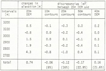
From Table I, we notice that the discrepancies between the results from the 20 m DEM and 10 m contours are small in general and the discrepancies for the other data sets are, as we might expect, somewhat bigger. In Table II, the changes in volume derived from the 20 m DEM and the discrepancies between these results and the changes in volume from the other data sets are given, for the 100 m intervals and for the total area, in a similar way as in Table I.
Table II Changes in Volume Derived from 20m DEMs and Discrepancies between this and the Changes in volume Obtained by using Contours and a 40m DEM.
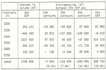
We notice that the discrepancy between the results from the 20 m DEM and the 10 m contours for the total area is very small. For the single intervals, the discrepancies are somwhat bigger, especially for the interval 3100-3200 m, for which the change in elevation is relatively small. That means that the relative error of the difference volume is bigger in this case compared with that of the other intervals. In addition, the changes in volume derived from contours are not only influenced by the original measurements, but also by the random error of the planimetry, which is also relatively great when the changes in elevation are small.
In Table III, the times required for the generation of the different data sets and the determination of the changes in volume and elevation are given. The latter task includes planimetric work and calculations For the contour method and program control and computational time for the DEM method. The times given for the 20 m and 50 m contours and for the 40 m DEM are estimated from the required times of the 10 m contours and the 20 m DEM, respectively. Considering both accuracy and economy, we notice that the results from 10 m contours and the 20 m DEM differ little, but using the 20 m DEM leads to much better economy.
Table III Time Requirement of the Different Methods.
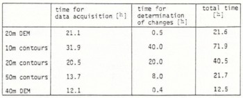
From Table III, we also notice that the time required for the 20 m DEM is the same as for 50 m contours, but the results from the 50 m contours (see Table I and II) differ a lot from the more dense data sets such as the 20 m DEM and the 10 m contours. Finally, the accuracy of the results obtained front the 50 m contours and the 40 m DEM is about the same, but with better economy in the case of the 40 m DEM. Consequently, the determination of changes in volume and elevation, using DEMs, leads to much better economy than using contour plots.
Determination of Changes in Volume and Elevation for the whole Vernagtferner Area using Digital Elevation Models
For the whole Vernagtferner area of 4960 x 3680 m2, the following data were measured, as described in chapter 2:
-
1979: 27 655 intersection points of 20 m contours with a 40 m grid; 1236 points along the borders of the glacier area.
-
1982: 15 336 reference points, measured using the method of Progressive Sampling; 2043 points along the borders of the glacier area.
With these input data, in both cases, a 20 m DEM was interpolated (46 065 points). From these DEMs, the changes in volume and elevation were derived for the glacier area, limited by the outer edges of the glacier in both years. Table IV includes these changes in volume and elevation, derived from the 20 m DEMs for 1979 and 1982, for all 100 m intervals and for the whole area.
Table IV Changes in Volume and Elevation for the whole Vernagtferner Area between 1979 and 1982 Derived from 20m DEMs.
The results show a decrease of the glacier in the upper regions and an increase below, which was also recognized qualitatively in Rü. Reference FinsterwalderFinsterwalder (1985), with another method.
The calculated change in volume can be used for the determination of the mass balance of the glacier, using the photogrammetric method as described in Reference PatersonW.S.B. Paterson (1969).
Conclusion
In the presented paper, a method for the determination of changes in volume and elevation, using Digital Elevation Models, was introduced and applied. It could be shown that this method leads to about the same accuracy as the traditional contour method, but with an enormous economic gain, because no additional planimetric work is needed. Furthermore, the DEM now available allows for various applications such as:
-
perspective views of the terrain
-
orthophoto and stereo-orthophoto profiles
-
general profiles
-
contour plots of desired interval
-
slopes and slope maps
All these products are readily available from the DEM without additional measurement. These various possible applications, together with the greater economy, demonstrate that Digital Elevation Models are recommendable for glacier research.


