1 Introduction

Conventional radio echo-sounding through ice sheets measures range to a reflector, leaving an ambiguity in position. When mounted on a moving platform, such as a sledge or aircraft, a two-dimensional representation of reflector range against along-track distance is obtained. If the reflecting surfaces are relatively smooth, their range will be a close approximation to nadir distance, and errors due to contributions from side echoes will be negligible. For steeper slopes, strong reflecting points give characteristic hyperbolic echoes of range against distance that allow these points to be identified and the reflecting surface to be more accurately reconstructed (Reference HarrisonHarrison 1971). There still remains the uncertainty about topography to the sides of the track and the effect of cross-track slopes. However, statistical analysis of the variation of echo strength with range and position can give an indication of the type of reflecting surface being observed and can allow different types to be discriminated (Reference BerryBerry 1975; Reference OswaldOswald 1975; Reference NealNeal 1979). Despite the promise of these methods in helping to unravel sub-ice conditions, in practice little has been achieved in applying them to problems such as identifying geological boundaries between nunataks. There are several reasons for this lack of progress, among them being uncertainty about the relationship between the radio-echo reflecting surface and the bed lithology. The presence of water and till at or near the base of the ice sheet could provide complicated reflecting surfaces that would not necessarily be characteristic of the underlying bed.

In order to study some aspects of the basal reflecting surface in more detail, a synthetic aperture radar (SAR) was developed. The advantages of this technique are that a high resolution can be achieved and that a two-dimensional image of the reflecting surface is obtained (Reference KovalyKovaly 1976). In the usual echo-sounding equipment that is used to penetrate thick polar ice the resolution is limited by the transmitted pulse length. For pulsed radio-frequency radars operating at 60 MHz, the pulse length is typically around 0.3 μs, equivalent to 50 m in ice. For impulse radars the equivalent pulse length can be an order of magnitude less (e.g. 5 m for a single cycle at 35 MHz), but there is often a penalty of reduced power and system performance that limits the depth that can be penetrated. The theoretical limit to the resolution of a SAR depends on the radar frequency and is proportional to the physical size of the antenna (Reference KovalyKovaly 1976). At 120 MHz (the carrier frequency used in the equipment described here) the resolution would be about 1 m. However, the achievable resolution is usually degraded by other equipment parameters as well as by the requirements of data processing. It is worth noting that with a SAR the resolution can be made independent of range by varying the length of the synthetic aperture, in contrast to the range-dependent resolution of sideways-looking radars that use real aperture techniques.

Intensity variations across two-dimensional SAR images are caused by changes in the back-scatter coefficient of a rough surface. Because the back-scatter coefficient of most surfaces is a strong function of viewing angle, the resulting SAR image can often be interpreted by the eye in the same way as an optical image. However, if there are any significant topographic features within the images, then their position will be displaced because the radar can only measure range. This “layover” effect can give significant distortion in mountainous regions. Airborne and satellite-based SAR images of the Earth’s surface are often used as an alternative to aerial photographs or high-resolution optical images because active radars such as SARs can operate at night time and through clouds (Reference ElachiElachi 1980).

In order to achieve a given resolution, data must be collected along a track (or aperture) preserving both in-phase and quadrature components of the signal (unlike conventional radars which preserve only amplitude). For SARs mounted on moving platforms these requirements can lead to very high data rates and sophisticated processing equipment. Photographic techniques can be used to record data as a kind of hologram but complicated optical processors are required to decode the images (Reference Cutrona, Leith, Porcello and VivianCutrona and others 1966). For this initial study of the application of SAR to sounding ice sheets it was decided that a ground-based system with a simple method for recording and analysing wave forms was appropriate. The major question was whether a realistic image of the glacier bed could be obtained through the non-homogeneous ice sheet. Corrections had to be made when processing the signals to allow for ice density, anisotropy, and absorption affecting the ray path and signal strength. The successful conclusion to this feasibility study means that further development of recording techniques is worthwhile.

2 Principles of Ground-Based SAR

High-resolution images can be recovered from coherent radar data by analysing the complex echo signatures from individual ground cells. In airborne or satellite systems, the platform velocity generates a doppler frequency for each reflecting point which can be isolated and identified if data are collected over a long enough aperture (Reference HargerHarger 1970). However, a ground-based system (which is essentially static when each radar pulse is transmitted and received) must instead rely on the phase history to identify point targets. In both cases, to avoid ambiguity of reflecting points at equal ranges on either side of the ground track, the radar is arranged to look to one side only. Consider the geometry shown in Fig.1. The ground swath illuminated as the radar moves can be considered to consist of a number of pixels, size Δx by Δy. The cross-track resolution, Δy, is calculated from the requirement that two reflecting targets with a separation Δy satisfies the relationship

Fig. 1 Geometry of SAR sounding (without an ice sheet). A combined transmitter/receiver (Tx/Rx) aerial moves along a path at height H above the reflecting surface, at range R from pixels of dimension Δx by ∆y.

where v is the velocity of radio waves, τ is the pulse duration, and Θ is the angle of incidence (Fig.2). The crosstrack resolution therefore depends not only on the pulse length but also on the angle of incidence. The location of reflecting points in the y-coordinate is derived from the echo delay time.

Fig. 2 Resolution in the across-track direction is determined by the separation d between adjacent reflecting points P₀ and P. The transmitter/receiver aerial (Tx/Rx) broadcasts and receives a pulse of radio waves of duration τ = n_cf which travels with velocity v at angle of incidence Θ with the ground surface.

To locate reflectors in the x-direction, an appropriate reference function is defined as the complex conjugate of the expected return from a point target in a given pixel. The recorded echo signals are then cross-correlated with the reference function centred on each pixel in turn and the relative strengths of the reflected signals evaluated for each cell (Reference WuWu 1978). A two-dimensional map of echo strength is built up, with cells of size Δx by Δy. The along-track resolution Δx can be deduced from the amplitude spectrum of the cross-correlation result, which can be written as

where

is a scalar quantity which represents the magnitude of the echo received from a point P with range R from the transmitter/receiver after it has been cross-correlated with the reference function located at an offset x₀ from P. The length of the aperture is L, ω₀ is the angular frequency of the radar wave, and E_p is the amplitude of the echo. The function

is plotted in Fig.3. It is centred about a value x corresponding to the location of the reflector and its amplitude is proportional to the strength of the signal reflected from the target. The width of the sine envelope therefore defines the along-track resolution, Δx. Taking the nulls as defining the half-width, Δx is given by

Fig. 3 Amplitude spectrum of cross-correlation result. The symbols are defined in the text.

It can be seen that the resolution can be made independent of target range R by adjusting the length of the synthetic aperture L.

A similar expression can be derived for a doppler-orientated SAR, showing that the resolving capabilities are the same as for the phase-sensitive SAR. However, by cross-correlating the doppler frequencies as well as the phases of the echo signals, the along-track resolution can be improved by a factor of two.

3 SAR Sounding Through Ice: General Principles

The overall effect of an ice mass on a SAR is to move the ground swath closer to the radar than it would be in free space. But the variable nature of the physical properties of an ice sheet also have to be taken into account if a worthwhile resolution is to be achieved (i.e. better than 20 m). The increase in permittivity with depth further refracts the radar signals and alters the apparent position of the echo source. The speed of the signals also changes with depth and has to be included when calculating the delay time of an echo signal.

The errors introduced in estimating the horizontal range of a reflector by assuming the ice to have constant permittivity (i.e. constant density) instead of a variation with depth, depend on the angle of incidence and ice thickness. The range would typically be underestimated by 9 m for an angle of incidence on the ice surface of 70° in ice more than about 300 m thick. Similarly, the two-way echo-time delay would be about 0.3 μs longer for constant-density ice. These errors, which are mainly introduced within the firn layer, are virtually constant for ice depths more than about 250 m.

A significant restriction on the size of the ground swath that can be imaged through an ice sheet arises from the requirement that echoes from the surface do not obscure echoes from the bed. This requirement places an upper limit on the angle of incidence on the ice surface and is a function of radar height above the snow surface, of ice thickness and of density. A typical value for the maximum angle would be about 70°. The lower limit is set by the cross-track resolution. Once the greatest angle of incidence has been calculated, the length of the aperture (L) required to synthesize a ground swath to a given along-track resolution (Δx) is provided by the equation

where R is the greatest slant range of a pixel and λ_i is the wavelength of the radar waves in ice.

Corrections must be made to the echo amplitudes to allow for absorption, scattering, partial reflection at the air ice boundary, geometrical losses, and the antenna-gain pattern. Although the losses due to geometrical effects are the greatest, it is the antenna-gain correction which is most sensitive to the relative position of the radar and the target. Fig.4 shows that signals that originated from the centre of the ground swath could appear to be 14 dB stronger than those from the outer corner, mainly because of the angular dependence of the antenna pattern.

Fig. 4 Amplitude correction profiles for echo signals originating at the centre of the ground swath (a) and at an outer corner (b).

The rate of change of echo phase along the aperture determines how often successive soundings must be made. In most practical cases this separation between soundings reduces to λ_i/2, but shorter distances are preferable to avoid approaching the Nyquist sampling limit too closely. Any variation in the radar frequency will introduce errors, so limits can be put on allowable oscillator jitter and drift by considering the phase history of reflecting points. Typical figures would place jitter at less than 2 kHz, and drift at less than 2 Hzs⁻¹ for a radar operating at 120 MHz. These restrictions can be met by placing a crystal oscillator in a temperature-controlled environment.

4 Imaging a Grounding Line: Field Results

A coherent radar working at 120 MHz with a half-wave dipole mounted in a 90° corner reflector was used to survey a grounding-line region on Bach Ice Shelf, Alexander Island, in the Antarctic Peninsula (Fig.5). The snow surface was smooth and flat to within a small fraction of a wavelength. The in-phase and quadrature components of the receiver output were recorded on photographic film and later digitized.

Fig. 5 Location map of area of SAR survey.

Fig.6 shows the ground swaths mapped by the SAR during three sounding runs. The position of the grounding line was originally estimated by using a 60 MHz radar and by observing the presence of strand cracks, a diagnostic feature of tidal bending at a hinge zone (Reference SwithinbankSwithinbank 1957). The ice thickness was around 290 m and the length of the sounding runs varied from about 300 m to 350 m. Records were obtained every 10 cm of aerial movement long the runs.

Fig. 6 Plan view of sounding runs (full lines) and ground swaths (dashed lines). Grounding line is shown by dotted line.

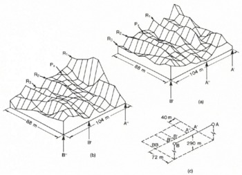
The digitized echo data were processed to give a chosen ground resolution of 8 m in both the along- and cross-track directions. The width of the ground swath that is mapped when sounding through 290 m of ice is 88 m and the length of the synthetic aperture needed to produce 8 m resolution in the along-track direction is 104 m. Thus, images containing 13 × 11 pixels are produced. Processing for higher resolution would give a narrower swath that also had proportionally fewer pixels. The values used here were chosen as a compromise between a high resolution with a narrow swath and a lower resolution that also gave a reasonable areal coverage. Because square pixels make subsequent analysis of the images easier to interpret, the pixel size in the along- and cross-track directions was chosen to be the same. Because the cross-correlation method does not consider the length of the transmitter pulse, the data can be processed to any desired resolution, but the measured pulse length of the transmitter, 140 ns, would give a nominal resolution across the track of about 30 m, thus blurring the image in that direction. Although the blurring is significant, it does not obscure the major details of the images.

The two images in Fig.7 were independently processed from data collected along the single traverse AB (Fig.6). Each image was derived from an aperture of length 104 m, but for the second image the aperture was displaced along track by 40 m (i.e. five pixels) with respect to the first. Although nearly 40% of the raw data are different in the two images, where they overlap, similar features can be identified. Ridges of relatively high signal back-scatter (R₁ to R₃): as well as an isolated peak P, are identifiable in both images. These features are displaced by 40 m, as expected if the processing were correctly computing aperture-averaged amplitudes of a spatially stable surface. Maximum amplitudes of ridges R₁ to R₃ in image (b) are 210%, 75%, and 76%, respectively, of the amplitudes image (a). This is the behaviour expected from linear reflectors such as ridges or troughs trending almost perpendicular to the traverse. As the viewing angle approaches the normal to the reflecting surface, a higher back-scatter will be produced. Thus, in Fig.7, ridges of high back-scatter increase in amplitude towards the ends of the aperture but are relatively low near the centre. (Note that the images are of signal back-scatter, not of topography.)

Fig. 7 Two images of echo strength taken along the same traverse (AB in Fig.6). Fig.7(b) is displaced by 40 m (five pixels) along track compared to Fig.7(a), as shown by sounding geometry in Fig.7(c).

The three images of the ground swaths in Fig.6 are shown in Fig.8. Each image was built up of smaller overlapping images, derived by processing successive apertures of length 104 m shifted 8 m (one pixel cell) along track each time. In the final (composite) image, each pixel value is the average of the individual image values for that particular pixel. This procedure reduces noise (often known as speckle) in the final image, although results from individual apertures seem to contain little noise anyway.

Fig. 8 Images of echo strength for the three ground swaths shown in Fig.6.

Quantitative texture analysis was used to classify and separate automatically the different types of surface. The procedure was based on second-order grey-level statistics (Reference Haralick, Shanmugan and DinsteiriHaralick and others 1973) in which a set of grey-tone spatial-dependent matrices is computed from the original images (Fig.8). Four measures of texture defined from values of the elements in the matrices provide a set of numbers which describe and identify an image. These numbers, known as “identification vectors”, can be used to compare textures of SAR images. Because of the relatively small number of pixels in our SAR images, the “Min-Max” decision rule was used to classify the various textures (Reference Haralick, Shanmugan and DinsteiriHaralick and others 1973): accuracies exceeding 80% have been reported for this method. The images from traverses AB and EF were analysed by splitting both into three equal parts (i.e. six portions each 8 × 11 pixels in size). The Min—Max decision rule automatically classified the two image portions closest to A and to F as one category and the four remaining portions into a different category. We suggest that these categories correspond to the division between grounded and floating ice, respectively.

A consistent interpretation of the three images can be given by assuming that a boundary between grounded and floating ice crosses each image as shown in Fig.6, Traverse CD (Fig.6) runs approximately parallel to the grounding line so that the strong echoes in the upper half of the image originate from grounded ice and the weaker echoes result from increased specular reflection from floating ice. Traverses AB and EF are orientated at angles of about 57° and 117° , respectively, to the grounding line. Both of these images show a significant amount of radar back-scatter from beneath floating ice, in contrast to the image from traverse CD. This implies that the subglacial surface of the floating ice scatters back virtually no signal to the receiver when the radar is looking directly towards the grounding line, but scatters back significant energy when the radar views the grounding line obliquely. A plausible explanation is that as the ice flows into the sea it retains an imprint of the rock surface where it was last grounded. Grooves running in the direction of flow would return comparatively little incident radar signal when viewed along the ice-flow direction but would give stronger returns when viewed across the line of flow. The elongation across track of strong reflecting points is due to the length of the transmitter pulse.

5 Conclusions

A method of imaging subglacial topography by using phase-sensitive radio echo-sounding gives realistic results across a grounding-line area. The technique of looking to one side of a sounding run is similar to SARs used in aircraft and space satellites. Because the equipment was used on the ground in essentially a static mode, no doppler information was available as is the case when sounding from moving platforms. Instead, the phase history was used in an analogous cross-correlation procedure to reconstruct a two-dimensional image of the target back-scatter coefficient. Textural analysis of the resulting images automatically classifies the surfaces into categories that correspond to those derived from visual interpretation.

An alternative method of mapping bedrock characteristics by sounding over a square grid on the surface has been described by Reference Walford and HarperWalford and Harper (1981). Both the amplitude and phase information are used to reconstruct the glacier-bed geometry and reflection coefficient. However, a large area would be easier to survey with a side-looking radar. Both methods suffer from not considering polarization effects, although it is recognized that the polarization behaviour of the radar waves contains information not only on the birefringent properties of the ice through which the signals are propagating but also on the nature of the reflecting surface and englacial scatters (Reference DoakeDoake 1982, Reference Walford, Kennett and HolmtundWalford and others 1986).