Experimental set-up

Snow samples were collected from Patsio research station (32 4 5′ N; 7716′ E, 3800 ma.s.l.), Great Himalayan range, India, transported by air to the cold laboratory in insulated boxes and stored at −20°C. This snow was composed of fine grains with an average diameter up to 0.15 mm. A heat-flux apparatus consisting of an insulated box with a copper plate (1.0 × 0.30 m²) heated electrically at the base was used for TG experiments. Insulation (100 mm Styrofoam) at the bottom and sides allowed us to maintain a one-dimensional (1-D) heat flow and reduce lateral heat losses. A schematic of the experimental set-up is shown in Figure 1. The detailed design of the apparatus and lateral heat loss analysis is given in Reference Satyawali, Singh, Dewali, Kumar and KumarSatyawali and others (2008).

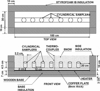
Fig. 1. Schematic of the experimental set-up (top and front views).

The apparatus was initially filled with snow to a height of 2 cm using a 1.0mm sieve opening. Next, seven thin, cylindrical tubes (diameter ∼2.2cm, height ∼4.3cm, wall thickness ∼0.6 mm) were carefully placed vertically on top of the 2-cm snow layer along the length of the heat-flux apparatus. The positions of the cylindrical tubes are shown in Figure 1. The heat-flux apparatus was then again filled with sieved snow very carefully to a total height of 10cm, such that the cylindrical tubes and the surrounding areas within the apparatus were uniformly packed with snow. Snow temperatures were monitored with type-T thermocouples placed at a regular vertical interval of 1 cm near the centre. The TG experiment was conducted for 6 days in a temperature-controlled cold room maintained at ∼–12°C with the snow surface exposed. The temperature at the bottom of the slab was maintained at ∼–2°C by the thermostatically controlled copper plate. The average temperature gradient across the snow slab during the experiment was approximately 96°Cm⁻¹, with a fluctuation of ±6.2°Cm⁻¹ due to fluctuations in cold-room (±0.9°C) and copper-plate (±0.5°C) temperatures. The embedded cylindrical samplers inside the apparatus were carefully extracted on a daily basis to examine the structural changes caused by the applied temperature gradient. The gap created by extraction of the samplers was refilled with similar snow by sieving.

X-ray microtomography imaging

Once sampled, each cylindrical sampler containing snow was weighted to calculate the density (ρ _s) of the snow. After weighing, the sample was imaged with a SKYSCAN 1172 high-resolution X-ray microtomograph. The objective of X-ray absorption tomography is to reconstruct the 3-D internal microstructure from the multiple X-ray shadow projection images recorded at different angular positions of the sample. In this work, 600 projection images covering 180° rotation around the vertical axis were obtained for each sample. The images were acquired with a pixel size of 8.56 μm from the mid-height of the sample. From the projection images, we reconstructed a cubic volume of interest (900 × 900 × 900 voxels) corresponding to a physical side length of 7.7 mm using modified Feldkamp cone-beam software (NRecon, SKYSCAN).

Representative elementary volume

The reconstructed 3-D images have an isotropic resolution of 8.56 μm, resulting in 900 × 900 × 900 images, which is a considerable quantity of volumetric data for processing. The resolution of the 3-D images was reduced by a factor of 3 in the three axes (300 × 300 × 300 voxels) to allow reasonable processing times for the microstructure parameters and the elastic properties computations. Therefore, for all the results presented in this paper, one voxel corresponds to 25.69 mm. The grey-level images were filtered with a 3³ median filter prior to image reduction. As the grey-level images showed adequate contrast, an automatic threshold using the histogram of the 3-D image dataset was applied to segment the ice and pore phases (Reference Seul, O’Gorman and SammonSeul and others, 2000).

To limit the computational time, the computational domain for both structural analysis and numerical simulation was chosen based on the following representative elementary volume (REV) analysis with respect to ice volume fraction (ϕ _i). ϕ _i was calculated using the hexahedral marching cubes volume model (Reference Lorensen and ClineLorensen and Cline, 1987) of the segmented ice phase. The variation of ϕ _i in cubic sub-volumes of increasing size within the reconstructed volume is shown in Figure 2a. A reasonable estimate for the REV of the investigated snow samples with respect to ϕ _i in this study was 60³ voxels or 1.54³ mm³ (Fig. 2a). We selected a computational domain of 100³ voxels (∼2.57³ mm³), which is more than four times larger than the minimal REV with respect to ϕ_i, for both the structural analysis and linear elastic properties computations. The structural indices were computed over nine different cubic sub-volumes (2.573mm3) within each reconstructed volume (7.73 mm³) to account for the statistical uncertainties. The location of sub-volumes within the reconstructed volume is shown in Figure 2b.

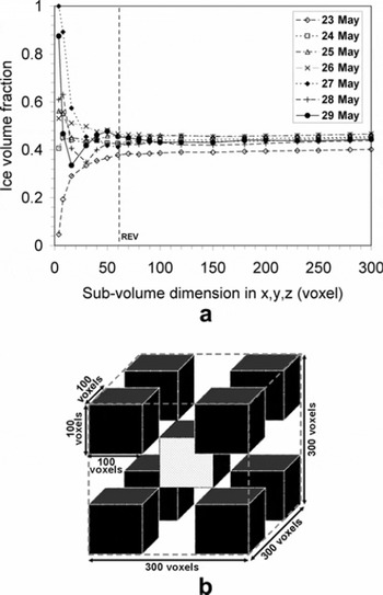
Fig. 2. (a) Variation of ice volume fraction as a function of increasing size of cubic sub-volumes within the reconstructed volume for REV analysis. (b) Locations of nine different sub-volumes (2.57 mm³) selected within the reconstructed volume (7.7 mm³) to account for statistical fluctuations.

Microstructure parameters

The SSA of the ice phase was determined based on the triangulated surface of the marching cubes volume model. The histograms of the local thickness distributions for the ice matrix (with mean structure thickness St_Th) and pores (with mean structure separation St_Sp) were obtained using the distance transform of the ice matrix and pore space, respectively (Reference Hildebrand and RüegseggerHildebrand and Ruegsegger, 1997b; Reference Remy and ThielRemy and Thiel, 2002). The structure model index (SMI) was computed based on dilation of the 3-D voxel model (Reference Hildebrand and RüegseggerHildebrand and Ruegsegger, 1997a). The SMI indicates the relative prevalence of rods and plates in the 3-D structure of the ice matrix. The geometrical degree of anisotropy (DA) was determined using the mean intercept length (MIL) method. The MIL is defined as the total length, L, of a line grid divided by the number of intersections between the grid and the ice/pore interface as a function of the grid’s orientation (ω): MIL(ω)= L/I(ω). The computed mean intercept length values were fitted to an ellipsoid and expressed as the quadratic form of a second-rank tensor M, i.e. a fabric tensor (Reference Harrigan and MannHarrigan and Mann, 1984). The MIL fabric tensor H is defined as the inverse square root of M. The advantage of using H is that larger values of H will be associated with larger values of Young’s modulus, and that the eigenvalues of H are the MIL values in the principal directions (Reference Odgaard, Kabel, van Rietbergen, Dalstra and HuiskesOdgaard and others, 1997). The principal intercept lengths (MIL1, MIL², MIL³) and the corresponding principal orientations were determined, and ordered such that MIL1>MIL²>MIL³. The degree of anisotropy is defined as: DA = MIL¹/MIL³.

The effect of resolution (three-fold reduction by resampling) on the evaluation of the structural parameters was tested for the snow samples at day 0 and day 2 (Table 1). Considering the three-fold decrease in resolution, the percentage changes in structural parameters are relatively small. Table 1 also shows the effect of measurement volume on the evaluation of structural parameters at resolution of 25 μm. Considering the 27-fold increase in measurement volume, the changes in structural parameters are relatively very small and our choice of a computational domain of 100³ voxels seems to fulfil the criterion of REV for the structural parameters considered.

Table 1. Effect of the resolution and measurement volume on the evaluation of structural parameters for the day 0 and day 2 snow samples

Computation of linear elastic properties

The linear elastic properties of snow were calculated from μCT data using a voxel-based FE programme (Reference GarbocziGarboczi, 1998). The FE method uses a variational formulation of the linear elastic equations and finds the solution by minimizing the elastic energy using a fast conjugate-gradient technique. To limit uncertainties, FE computations were also carried out over nine different cubic sub-volumes of 2.573 mm³ within each reconstructed volume (Fig. 2). The voxels in the μCT datasets were converted directly into trilinear isotropic brick elements. For ice, linear elastic and isotropic properties were specified with a Young’s modulus of 9.5 GPa and Poisson’s ratio of 0.3 (Reference Sanderson and SandersonSanderson, 1988). Six FE analyses were carried out for each sub-volume considered, with periodic boundary conditions and only one of the six independent strains (ϵ ₁, ϵ ₂, ϵ ₃, ϵ ₄, ϵ ₅, ϵ ₆) non-zero each time. The complete elastic compliance matrix (S_ijkl ) was then computed from the results of these analyses. Utilizing a numerical optimization procedure, the best orthotropic representation of S_ijkl was obtained and Young’s moduli (E ₁, E₂ , E ₃) and shear moduli (G ₁₃, G ₂₃, G ₁₂) were calculated (Reference Van Rietbergen, Odgaard, Kabel and HuiskesVan Rietbergen and others, 1996).

Microstructural changes under temperature gradient

The 3-D evolution of snow structure under applied temperature gradient is shown in Figure 3. For better visual perception, vertical slices (7.7 × 7.7 × 0.26 mm) in the central y-z plane of the complete reconstructed volume along with small sub-volumes (1.743mm3) are depicted. Visual inspection of the 3-D snow structure indicates a general coarsening along with the development of thicker vertically oriented ice structures, along the direction of the applied temperature gradient.

Fig. 3. Temporal changes in 3-D snow structure caused by temperature gradient metamorphism. Vertical slices (7.7 × 7.7 × 0.26 mm) in the central y-z plane along with smaller cubic regions (∼1.71³ mm³), are depicted.

The temporal variations in mean structural parameters during the experiment are shown in Figure 4. The error bars depicted in Figure 4 reflect ± 2 standard error and represent the statistical uncertainties between the analyzed sub-volumes. The statistical fluctuations are less than 2–7% for most of the data points. The density is probably one of the most significant first-order structural parameters of snow and is derived from the ice volume fraction ϕ_i. In this work, we computed p_s both by weighting of the cylindrical samplers and from ϕ _i using image analysis of the μCT voxel data. The μCT-based mean density values were higher than those obtained by the weighting method; however, the maximum relative difference was less than 7%. The density of the snow at the start of the experiment was ∼368kgm⁻³. The density varies in a complicated way during the experiment; initially, an increase was observed for the first 2 days and thereafter no significant trend was found (Fig. 4a). A maximum increase of 14% was noted immediately after the application of the temperature gradient on day 1 itself. The variations in structure thickness for ice and pores are depicted in Figure 4b. St_Th increased from an initial value of 0.151 ± 0.003 mm to 0.165 ± 0.004 mm on day 3 and then remained almost constant. St_Sp increased continuously from 0.171 ±0.006 mm to 0.228 ±0.008 mm at a much higher rate during the experiment. Figure 4c shows the changes in histograms of the local thickness for the ice matrix and pores. For better clarity, the histograms are shown only for the samples examined at initial day 0 and final day 6. While the pore-space thickness distribution increases and widens continuously, the ice matrix thickness histogram evolves at a much slower rate up to day 3 and hardly changes thereafter.

Fig. 4. Changes in the structural parameters during the temperature gradient experiment. (a) Density; (b) mean thickness of ice matrix and pores; (c) histogram of the local thickness for the ice matrix and pores; (d) mean intercept length (MIL) fabric measures; (e) structure model index (SMI) and degree of anisotropy (DA); (f) Specific surface area (SSA).

The changes in principal intercept lengths (MIL1, MIL², MIL3) of the MIL fabric tensor and the corresponding fabric anisotropy (DA) are shown in Figure 4d and e respectively. The evolution of the principal orientations of the MIL fabric tensor is given in Table 2. The principal intercept lengths are each an index of the relative length of ice intercepts in each of the three axes described by the orthogonal principal directions. It should be noted that the intercept length may correlate with object thickness in a given orientation but does not measure it directly. The primary direction of MIL fabric tensor (corresponding to MIL1) aligned itself vertically, i.e. in the direction of the applied temperature gradient within 1 day (Table 2). All three principal intercept lengths increased continuously up to day 3 and reached a plateau, albeit MIL1 increased at a 1.5- to 2-fold higher rate than MIL2 and MIL3. The maximum anisotropy was reached on day 3 and then remained almost constant. The values of MIL fabric tensor measures (Fig. 4d; Table 2) indicate a transversely isotropic fabric ellipsoid with primary orientation along the direction of the applied temperature gradient. It appears that as the structure becomes vertically oriented, the directionally averaged mean structure thickness obtained from the distance transformation method cannot capture the evolution accurately.

Table 2. Orthogonal principal orientations (direction cosines) of MIL fabric tensors

The SMI of the ice matrix decreased continuously from 1.86 at the start of the experiment to 0.43 on day 6, which is consistent with the formation of thicker, vertical plate-type ice structures (Fig. 4e). The evolution of SSA during the experiment is presented in Figure 4f. The SSA decreased by ∼22% by the end of the experiment, with maximum changes occurring within the first 3 days. Although the experiment was of only 6 days duration, Figure 4e indicates that the decrease in SSA of the ice matrix follows a logarithmic trend quite well.

The observed evolution of various structural parameters during the TG metamorphism in the present work appears to be in line with observations reported by Reference Schneebeli and SokratovSchneebeli and Sokratov (2004) for the high-density sieved snow, except for the SSA; Schneebeli and Sokratov noted that SSA decreases only for the low-density snow samples, not for the high-density snow samples.

Linear elastic properties

The variations in computed Young’s moduli (E ₁, E ₂, E ₃) during the TG experiment are shown in Figure 5a. Like the fabric eigenvalues (MIL₁>MIL₂>MIL₃), the compliance matrix was sorted such that E ₁>E ₂>E ₃. Implicitly, it is assumed that the principal mechanical directions are closely aligned with the principal fabric directions. It is interesting to note that the temporal variation pattern of maximum Young’s modulus E ₁ is closely related with many of the structural indices. The Young’s modulus (E ₁), oriented along MIL1, increases from 459.2 ± 26.2MPa on day 0 to 1007.0 ± 55.2 MPa on day 3, and thereafter remains more or less constant. The maximum increase in E₁ of more than 100% was observed on day 1 itself. Young’s moduli E₂ and E₃ increased by about 40% on day 1 and then slightly decreased to reach a plateau. The similarity in estimated values of E₂ and E3 indicate a transverse isotropic compliance matrix. The variation in shear moduli (G ¹³, G23, G ¹²) was similar to Young’s moduli (Fig. 5b), with maximum changes in shear moduli occurring within 1 day. The error bars depicted in Figure 5 represent the statistical uncertainties between the analyzed sub-volumes.

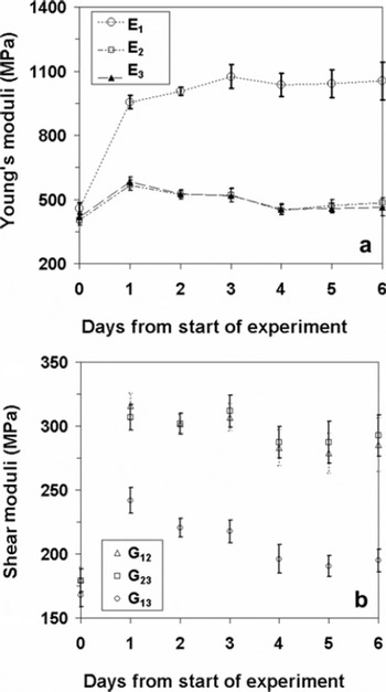
Fig. 5. Variations in computed elastic moduli during the temperature gradient experiment. (a) Young’s moduli (E ₁, E ₂, E ₃); (b) Shear moduli (G ₁, G ₂, G ₃).

Reference SchneebeliSchneebeli (2004) computed the evolution of Young’s modulus of snow (density -243 kgm⁻³) in a TG (100°Cm⁻¹) experiment using FE analysis of μCT voxel data. He found a substantial decrease (>70%) in axial Young’s modulus after 6 days; however, correlations with structural changes were not reported. Although the 3-D structure becomes progressively coarser, the formation of vertical ice structures was not observed (fig. 1 in Reference SchneebeliSchneebeli, 2004). Interestingly, Reference Schneebeli and SokratovSchneebeli and Sokratov (2004) found that the effective heat conductivity (EHC) of high-density (490–514 kg m⁻³) sieved snow samples under strong temperature gradients increased immediately; EHC almost doubled from the initial value and reached a plateau at constant density. The increase in EHC was attributed to the formation of thick, vertical ice structures during recrystallization. Reference AkitayaAkitaya (1974) observed the formation of a very hard, cohesive type of depth hoar when snow (ρ _s > 300 kg m⁻³) was exposed to temperature gradients >39°Cm⁻¹. Reference Pfeffer and MrugalaPfeffer and Mrugala (2002) also demonstrated that hard depth hoar forms from rounded-grain snow (ρ≥400kgm⁻³) following exposure to temperature gradients >20°Cm⁻¹. They characterized hard depth hoar as solid-type depth-hoar grains connected by necks, with vertically preferred directions of grain elongation using horizontal and vertical section planes. The increase in computed elastic moduli during the TG experiment found in the present work is in qualitative agreement with the formation of thicker vertically oriented ice structures (Fig. 3), parallel to the direction of the applied temperature gradient. It appears that both the increase in Young’s moduli in the present work and the increase in EHC, as reported by Reference Schneebeli and SokratovSchneebeli and Sokratov (2004), are related to the formation of hard depth-hoar-type structures when high-density sieved snow samples were subjected to high temperature gradients.

Combining entire structural analysis and FE computation datasets, non-parametric Spearman’s rho correlation coefficients (R ²) were determined between elastic compliances and 3-D structural indices (Table 3). R ² gives the proportion of variance explained by the independent variables. Primary Young’s modulus (E ₁) and shear moduli (G ₁₂, G23) were correlated significantly with the structural parameters, unlike E ₂, E ₃ and G ₁₃, which show poor or no significant correlations. In summary, high correlations (R ₂= 0.71–0.87) were obtained for the ice volume fraction, and modest to high correlations (R ₂ = 0.3–0.76) were found for structural parameters. Compared with shear moduli (G ₁₂, G ₂₃), E ₁ was found to be better correlated with MIL fabric measures (MIL_i and DA). Distance transform-based ice and pore-thickness measures, as well as specific surface area, appear to be modestly correlated with elastic moduli. However, it should be noted that the structural parameters considered here are not completely independent and are related to each other.

Table 3. Non-parametric Spearman’s rho correlations (R ²) between mechanical properties and structural parameters

We have compared our numerical estimates with theoretical Hashin–Shtrikman (HS) bounds (Reference Hashin and ShtrikmanHashin and Shtrikman, 1963) and previously reported dynamic measurements. The HS bounds are probably the best bounds on the properties of a two-phase composite material without specifying any structural information beyond solid volume fraction or porosity. Figure 6a shows the comparison of the estimated Young’s moduli with the upper HS bound and experimental values reported in Reference Maeno, Narita and AraokaMaeno and others (1978) from the transversal vibration method. The simulated Young’s moduli were 2–8 times less than the theoretical HS bound and 1.5–4 times larger than the dynamic measurements. As such, direct comparison of FE estimates with reported values is difficult because the complete elastic stiffness matrix was not measured for snow and the reported results come mostly from quasi-static compression tests assuming an isotropic material. The error in quasi-static compression tests might obscure the true elastic response and reduce the effective stiffness of the material. Moreover, reported values of effective Young’s modulus are strongly dependent on strain rate and our FE analysis does not take into account the strain-rate dependency. Figure 6b shows the comparison of computed shear moduli with the theoretical upper HS bound. The computed G_ij values were 3–7 times smaller than the HS bound. The scatter in Figure 6 represents the evolving mechanical anisotropy during the TG experiment.

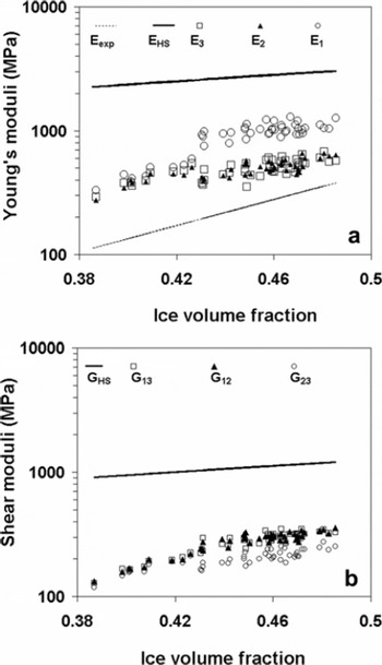
Fig. 6. (a) Comparison of Young’s moduli with Hashin–Shtrikman (HS) upper bound (E _HS) and dynamic measurements (E _exp) of Reference Maeno, Narita and AraokaMaeno and others (1978). (b) Comparison of shear moduli with HS upperbound (G _HS).

Developing relationships between material morphology and mechanical properties is of prime importance in many other research areas, such as bone biomechanics. Reference CowinCowin (1985) developed a polynomial relationship between elastic properties (nine orthotropic elastic constants) and the structure, given by volume fraction and a fabric tensor. Reference Kabel, van Rietbergen, Odgaard and HuiskesKabel and others (1999) developed constitutive relations of fabric, density and elastic properties in cancellous bone. Based on the elastic-properties-fabric model derived by Cowin, we also attempted to relate the normalized MIL fabric eigenvalues and ice volume fraction 4> _i with the nine orthotropic elastic compliances obtained from the FE analysis. The relationships for the elastic compliances (S_ijkl ) are:

(1)

where i, j = [1, 2, 3], i ≠ j and Ψ = λ₁λ₂ + λ₁λ₃ + λ₂λ₃.

The constants appearing above were calculated by independently fitting each relation using non-linear multiple regression analysis (Table 4). Figure 7 shows the plots between the compliance coefficients obtained from FE analysis and the compliance coefficients predicted by the above relationships. The regression model based on MIL fabric measures and ice volume fraction explained 89.9–93.0% of the variation of the elastic compliances.

Table 4. Values of constants appearing in regression models (Equation1) obtained from the independent fits

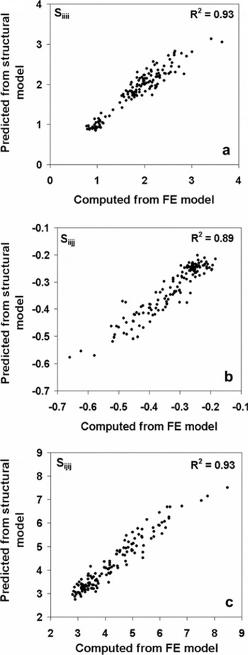
Fig. 7. Correlation between the calculated (from FE technique) and predicted (from regression model) compliance components. (a) S_iiii ; (b) S_iijj ; (c) S_ijij .

Finally, some points regarding three sources of errors, i.e. finite size effects, statistical fluctuations and discretization errors, in the structural and FE analysis should be noted. We have not carried out a detailed error analysis for FE computation due to limitations of computational speed. Structural analysis (Fig. 2a; Table 1) showed that the selected computational volume respects the REV criteria for determination of structural parameters. Correlation analysis (Table 2) suggests that the ice volume fraction is one of the significant parameters controlling the elastic properties. As the computational domain for elastic properties estimation is about four times larger than the minimal REV with respect to ϕ_i, we presume that the finite size errors in FE analysis are also small. Reference Kaempfer, Schneebeli and SokratovKaempfer and others (2005) found a REV of 5₃ mm₃ with respect to heat flux in the ice matrix, which is about seven times greater than the computational volume used in this work. Averaging of parameters using nine sub-volumes within the reconstructed volume produces an acceptable level of statistical uncertainties (2–7% for structural parameters and 5–17% for the elastic moduli computation). The discretization error is due to the use of discrete voxels to represent continuum structures. Table 1 shows that the discretization error at a resolution of 25.69 mm is relatively small for the measured structural parameters. Using a periodic open-cell strut model, Reference Roberts and GarbocziRoberts and Garboczi (2002) showed that the discretization errors are <10% if the strut thickness is covered by a minimum of four voxels. In the present work, with the determined minimum mean ice structure thickness of St_Th = 0.151 mm at a resolution of 25.69 μm, we obtained a discretization of a minimum of six voxels per ice structure thickness which meets the criteria established by Reference Roberts and GarbocziRoberts and Garboczi (2002).