Introduction

The Hamburg Ocean Primitive Equation (HOPE) model has already been used in coupled ocean�atmosphere experiments investigating equatorial and low-latitude dynamics on a decadal time scale (e.g. Reference LatifLatif and others, 1994). In these experiments, sea-surface temperature (SST) and sea-surface salinity (SSS) are relaxed to climatological data at high latitudes. At these latitudes, however, water masses are formed that ventilate the deep ocean. Since die sea-ice cover effectively modifies the momentum, heat and freshwater exchange between the atmosphere and the ocean, it should be accounted for in the coupled atmosphere-ocean models that will be used in long-term integrations of the climate system.

In order to allow the HOPE model to become a component in a coupled ocean-atmosphere model for studying climate, it has been coupled to a prognostic dynamic-thermodynamic sea-ice model. The sea-ice cover of a 1000 year spin-up experiment is described in the third section. In general, the performance of the model is satisfactory. In the Southern Ocean, however, die ice cover predicted by the model is loo thin and the minimum ice extent is loo small. This is due to excessive upward oceanic heat flux occurring during the convective adjustment of hydrostatically unstable water columns. the static stabitity of the upper ocean in ice regions depends on the vertical distributton of salt, which is strongly influenced by haline rejectton during ice formatton. Because of die lack of reliable fresh-water flux data, and in order to prevent the ocean model drifting into an unrealistic climate scenario, global ocean models are frequently driven with salt or fresh-water flux derived from relaxing SSS to observed data. In coupled ice-ocean models, this might seriously affect the salt flux by haline rejectton at the ice-ocean interface. In the fourth section, the influence of different treatments of SSS and rejected brine on the ice cover, water mass characteristics, and circulatton in the Soulhern Ocean are described.

Model Description

Details about the numerical formulation of the ocean and ice model are given in a technical report (Reference Wolff, Maier-Reimer and LegutkeWollf and others, 1997). The ocean model is based on primitive equations that are diseretised on a spherical global grid. The non-linear equations are solved on 20 unevenly spaced horizontal levels. The level separations increase with depth (10 levels in the upper 250 m) in order to give a better representation of the more variable upper ocean. The first layer has a thickness of 20 m. Since the height of die deepest box in each column can be adjusted so that the sum of die height of all overlying boxes equals the total water depth, the representation of bottom topography depends on the horizontal resolution of the model grid only. For the horizontal discretisation, a staggered grid (Arakawa-E) is used with a 2.8° zonal and meridional gridpoint distance in mid and high latitudes. This corresponds to the grid of the atmosphere model that produced the forcing data. To be able to investigate natural variabitity in the Equatorial ocean, however, the ocean model resolution is increased in low latitudes. The meridional gridpoint separation decreases equatorward of 30° north and south, reaching its minimum of 0.5° at 10° north and south. Prognostic variables of the ocean model are potential temperature, salinity horizontal velocities and sea-surface elevation. Potential density is computed with die non-linear UNESCO formula, and vertical velocity is calculated from the incompressibility equation for sea water. Sub-gridscale mixing is parameterised by horizontal harmonic diffusion terms with the coefficients depending on the horizontal velocity shear. Vertical viscosity and diffusivity depend on the local Richardson number. In cases of hydrostatically unstable stratification, “convective adjustment” takes place (that is, vertically adjacent gridboxes with unstable stratification are mixed).

The dynamic part of the ice model is based on the Reference HiblerHibler (1979) sea-ice dynamics that are reformulated on the occanmodel grid (i.e. the ice behaves like a viscous-plastic material with an elliptic yield curve). A 2-layer ice formulation is used for the dynamics and thermodynamics, and in each gridcell thin ice (open water) and thick ice can be present. Following Reference Parkinson and WashingtonParkinson and Washington (1979), ice growth and melt is calculated from heat-budget equations based on simple bulk formulae for the turbulent and radiative heat fluxes over water and ice, as described by Reference Stössel and OwensStässel and Owens (1992). A prognostic snow layer is also included.

The coupled model integration was initialised with the Reference LevitusLevitus (1982) climatology, and with the ocean and ice velocities at rest. the initial ice thickness was specified to decrease from 2 m at the northernmost/southernmost ocean cell to 0 m at the latitude of the observed ice edge. A 1000 year integration has now been completed. It has been forced with a 15 year period of daily data of net atmospheric heat flux. 2 m temperatures and dew points, cloudiness, precipitation�evaporation, continental runoff, and windstress. They were produced by the ECHAM4 atmosphere model, which was run with a 2.8° resolution and climatological SST of the Atmospheric Model Intercomparison Project (AMIP) period (1979–88) as lower boundary conditions. The ECHAM4 model and its performance are described in Reference Chen and RoecknerChen and Roeckner (1996). A running-mean fitler of varying length has been applied to the first and last 10 days of the 15 year period in order to eliminate sudden changes of the forcing when it is cyclically repeated.

In order to prevent the ocean from drifting into a climate state that is different from the present, the SST is relaxed to the monthly AMIP SST with a relaxation constant of 40W/(m² K) corresponding to a time-scale of 24 days. The atmosphere model fresh-water flux (P-E) and runoff) is modified by an amount that changes the upper-ocean salinities as if they were relaxed to the annual mean of the Levitus climatology on a 30d time-scale. This is only applied outside the ice regton as defined by the AMIP data, so that the salt fluxes caused by the freezing and melting of sea ice are not disturbed.

After the 1000 year integration, the model fields are almost cyclo-stationary (that is, the drift of level mean salinities is O(10⁻³ psu/(100 a)). The main oceanic water masses and currents are reproduced. The Pacific- equatorial current system is shown in Reference Legutke, Maier-Reimer, Cubasch, Stössel and HellbachLegutke and others (1996). The Gulf Stream, Kuroshio and Antarctic Circumpolar Current (ACC) have mean transports of 32, 50 and 110 Sv, respectively. The maximum overturning transport in the North Atlantic is 15 Sv of which 10 Sv are leaving at 40° S. The Indian and Pacific oceans are ventilated by 5 Sv each, which are flowing northwards in the deep layers from the Southern Ocean. The Pacific-Indian throughflow amounts to 13 Sv; 12 Sv are entering the South Atlantic in the Agulhas Current. These transport values are consistent with observations.

In general, the model generates data where the deep ocean tends to be too fresh and too cold, and mean level salinity and temperature are 0.06 psu and 0.4°C below values predicted by the Levitus climatology. In the upper ocean, the errors are of the same order but too warm and too saline. The greatest errors occur in oceanic mid-depths (0.27 psu) due to problems in representing accurately the Antarctic and North Pacific Intermediate Water, the simulated salinity of which is about 0.3 psu too high.

Sea-Ice Cover of the Long-Term Integration

In this section, we describe the ice cover between the years 1000–1014 (mean of one forcing period) of the spin-up run. The computed 15 year mean seasonal cycle of Arctic ice extent compares reasonably well with observations (Fig. 1) although the winter-ice extent is overestimated. Note, however, that the ice extent tends to be overestimated if it is computed from data averaged over a long period, and if there are regions where the position of the ice edge changes from year-to-year. In February, ice concentration is above 95% in the central Arctic while in September, 5–10% of the water is free of ice. Towards the coast, the fraction of open water increases (this can be as high as 70% in the Kara Sea). Off Greenland and the Canadian Archipelago, the ice cover remain compact (>95%) all year due to ice convergence (not shown).

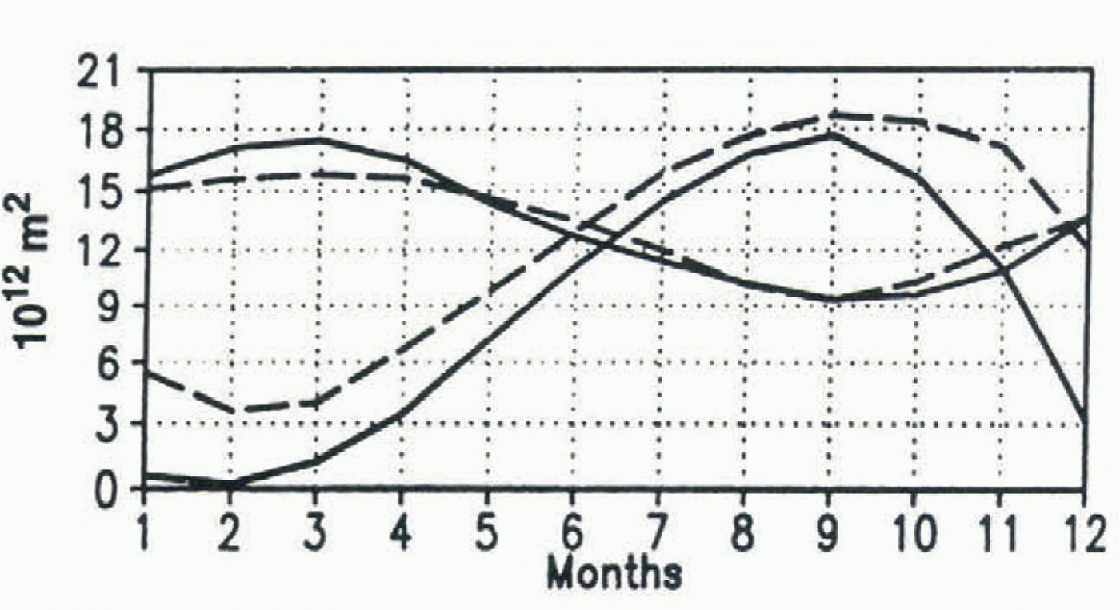
Fig. 1. Seasonal cycle of observed (dashed line) and simulated (full line) ice extent of the Northern and Southern Hemi-spheres. The observations are reproduced from Reference Gloersen, Campbell, Cavatieri, Comiso, Parkinson and ZwallyGloersen and others (1992).

The model also shows the ice as too thick in northern Baffin Bay, which, at least partially, can be attributed to the coarseness of a model grid that does not allow for an appropriate heat flux from the North Atlatitic nor from the central Arctic into this region. Regions of increased ice thickness also exist off Greenland and the Canadian Archipelago, which is consistent with observations. A second region of thick ice predicted by the model is found in the East Siberian sector of the central Arctic, white thin ice is present near the Bering Strait and in the Beaufort and the Kara Seas. This distribution is similar to that computed by Reference Flato and HiblerFlato and Hiber (1995) with observed atmospheric-pressure analyses from 1979 to 1985.

Mean upward oceanic heat flux in the central Arctic is estimated to be about 2 W m⁻² (Reference Maykut and UntersteinerMaykut and Untersteiner, 1971), with much higher values (30 W m⁻²) in the Eurasian Basin (Reference Aagaard and GreismanAagaard and Greisman, 1975). The modelled-area mean upward heat flux in the ice region is 10–25 W m⁻² during the freezing season (not shown).

The Southern Ocean winter-ice extent is in reasonable agreement with observations, but in the other seasons it is severely underestimated (Fig. 1). Due to weaker stratification, the upward heat flux in the Southern Ocean is much larger than in the Arctic (Fig. 2). Annual mean heat flux estimates for the Southern Ocean ice region are about 30 Wm⁻² (Reference GordonGordon, 1981). As in the Arctic, the convective-adjustment heat flux is highest in the freezing season. The largest values occur in the Weddell and Ross Seas. This is reflected by the mean Septemher ice concentration: in the eastern part of the Weddell Sea it is below 20%, while in the Ross Sea, there is a large region with no iee at all (Fig. 3).

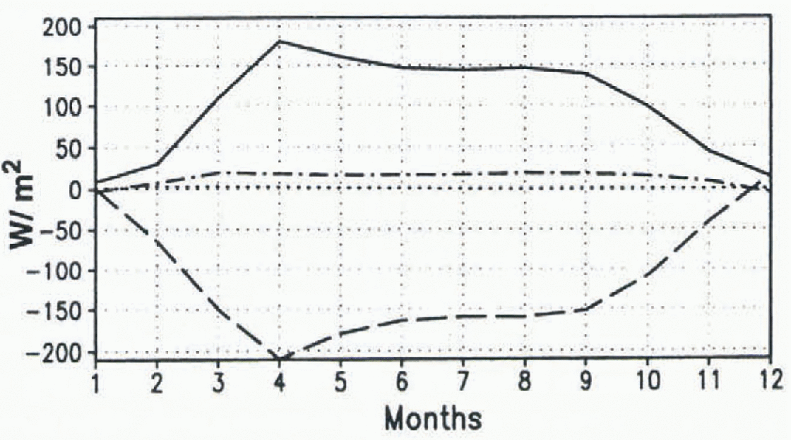
Fig. 2. Seasonal cucle of heat fluxes into the upper ocean layer in the ice region of the Southern Hemisphere. Convective adjustment is the full line; vertical diffusion is the dot-dash line; upwelling and horizontal advection and difusion is the dotted line; atmosphere is the dashed line.

Fig. 3. Mean (years 1000–1014) simulated ice concentration in the Southern Hemisphere in September. Contour lines are 0,20,40,60,80 and 90%.

The mean September ice thickness is underestimated by a factor of ∼2 (not shown).

Sensitivity Experiments

Since salinity dominates potential density at low temperatures, it is the destabitisation of the upper ocean by haline rejection that causes the overturning, and is thus responsible for the strong upward oceanic heat flux. This is demonstrated by the geographical distribution of ice compactness in an experiment where the salt flux during ice melting or freezing was turned off (Fig. 4). The September ice cover is shown to be compact almost everywhere (except near Cape Norvegia at 0°E; in this area large off-shore polynyas are frequently observed). This distribution relates much better to observations (Reference Gloersen, Campbell, Cavatieri, Comiso, Parkinson and ZwallyGloersen and others, 1992). The frequently observed regions of reduced ice concentration or open water adjacent to the coast, which were reproduced by the long-term experiment described in the prevtous section, however, are now missing. The ice is thicker than 60 cm in the region where the ice concentration is above 80%, reaching values of about 1 m near the coast and up to 2 m at the east coasts of the Weddell and Ross Seas (not shown).

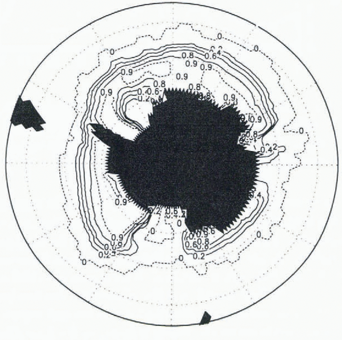
Fig. 4. Mean (years 76–90) simulated ice concentration of exp16 (no brine release) in the Southern Hemisphere in September. Contour lines are 0, 20,40,60,80 and 90%.

In order to see the impact of other treatments of the SSS in use by ocean modellers, we gradually increased the impact of brine release during freezing in several experiments. In one experiment (named exp12), SSS were relaxed to climatological values everywhere. In a second experiment (exp11) the salinity of sea ice was increased from 5 to 32 psu. A third experiment (exp09) relaxed the SSS on the ice-free part of each gridcell only, while in a fourth experiment (exp05) SSS was not relaxed in the climatological ice region and was run long-term. In a fifth experiment (exp10) relaxation was not applied at all while in the last experiment (exp06) 30% of the brine released during Iteezing was immediately transferred to level 2 of the ocean model. After about 45 years of integration, the ice cover reached a nearly cyclo-stationary stale in all experiments. In general, the ice area decreased in the order the experiments are listed above (with the exception of exp06) (Fig. 5). Thus, the more the brine release becomes important, the less ice was present. None of the experiments, however, realistically reproduced the observed summer ice area of at least 2 × 10¹² m¹² Reference Gloersen, Campbell, Cavatieri, Comiso, Parkinson and ZwallyGloersen and others, 1992).

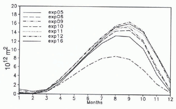
Fig. 5. Mean (year 76–90) seasonal cycles of ice area in the Southern Hemisphere (gridbox area multiplied by compactness) of the sensitivity experiments. The experiments are explatned in the text.

The ice areas of the experiments are similar from January to June with the exception of exp10 (no relaxation). The experiments with no brine release, salty ice, and relaxation of SSS to climatologies in all gridcells also have similar values from July to December. The upward oceanic heat fluxes simulated in the experiments are displayed in Figure 6. Large values correspond to small ice areas. The experiment without SSS relaxation (exp10) has mean heat-flux values of more than 150 W m ⁻² from April to September, which is far above observational values. The salinity relaxation equatorward of the ice edge is necessary to keep the SSS low there. This is probably due to the low ice production near the coast that does not provide enough ice For melting further offshore.

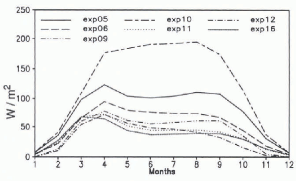
Fig. 6. Mean (years 76–90) seasonal cycle of oceanic heat flux by convective adjustment in the ice region of the Southern Hemisphere. The experiments are explatned in the text.

Of course, the heat flux is not without influence on the temperatures of the deep water masses. Mean temperature profiles of the Weddell and Ross Seas are shown in Figure 7. None of the experiments could reproduce the observed (full thick line pronounced temperature maximum at 800m in the Weddell Sea though exp05, exp06, and exp09 display a weak maximum at this level. The salty-ice (dotted), the no-relaxation experiment (short-long dashed) and the no-brine experiment (short dashed) have their maxima located too high in the water column. The profiles are well-mixed down to the bottom except in experiments with salinity relaxation in the ice region (exp09 and expl2), where the overturning reached only 2000 m resulting in second deep maxima. In the Ross Sea. the profiles are belter reproduced, except agatn in those experiments with salinity relaxation in the ice region. The best fit is obtatned when 30% of the rejected brine is immediately transferred to the second model layer, In this case, less frequent overturning of the fresh and cold surface water results in saltier and warmer deep water.

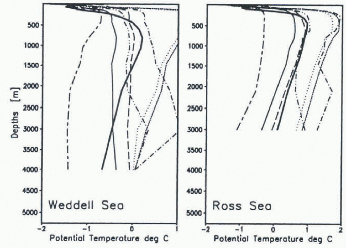
Fig. 7. Mean (years 76–90) temperature profiles in the Weddell and Ross Sens. The contour styles correspond to the same experiments shown in Fig.5. The thickfull line is derived from the Levitus climatology.

The influence of the treatment of SSS on the strength of the ACC is demonstrated by the time series of volume transports in the Drake Passage (exp05 and exp12 Fig, 8). After an initial decrease during the first 60 years, the time series are cyclo-stationary, reflecting the repeated application of the 15 years of forcing data. We see a pronounced difference between the two time series in the strength of the 15 year cycle. Obviously, on this time-scale, the thermohaline forcing of the circulation (via brine release and subsequent Overturning) through the so-calledJEBAR (Joint Effect of Baroclinicity and Bottom Relief) dominates. This constitutes a positive torcing of the ACC Large-scale global circulation is, of course, also influenced by the SSS boundary condition (the more rigorous overturning in the Southern Ocean in exp05 results in a global meridtonal overturning cell in the deep ocean that is twice as strong as that in expl2 (not shown)).

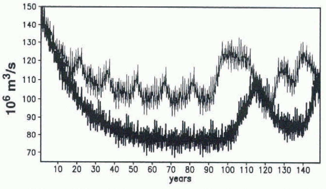
Fig. 8. Time series of monthly mean volume transports of the ACC in exp05 (thin line) and exp12 (thick line).

Some modellers use fresh-water fluxes diagnosed in prevtous experiments with salinity relaxation to drive their ocean (-sea-ice) model. In order to assess the impact of annual mean fresh-water fluxes diagnosed with different treatnment of SSS, some of the experiments were continued to year 150 with the salinity-relaxation surface-boundary condition replaced by the 15 year mean fresh-water flux of years 76–90 as diagnosed in the experiments described above. With the beginning of the use of time-constant fresh-water forcing, new internal time-scales of about 30 years come into play. They are superimposed on the 15 year and short-term fluctuations forced by the atmosphere model data with even larger amplitudes. the strength of the ACC is strongly correlated with the sea-ice volume on longer time-scales with the latter leading some years not shown).

Conclusions

A coupled world-ocean sea-ice model has been integrated for 1000 years Itirced by 15 years of daily atmosphere model data. The observed mean state of the ocean is reasonably well reproduced, as is the ice cover of the Northern Hemisphere.

In the Southern Hemisphere, however, the predicted values show that the ice is too thin and the summer ice extent too small. This can be attributed to excessive oceanic heat flux by convective adjustment in the ice region caused by rejection of brine during the freezing of sea ice. Reference MartinsonMartinson (1990) has shown that with the temperature and salinity stratiticalton in the Southern Ocean, open-ocean convection acts as an upward pump of salt and heat. This is also the case in our model with. however, open-ocean convection extending to the bottom. If, on the other hand, we try to reduce the convective adjustment (e.g. by relaxing the SSS to the Levitus climatology, which induces a fresh-water flux), the deep ocean warms up excessively. The upper 1000–2000 m become fresher than without relaxation due to the continuous flux of fresh water and the reduced overturning depth. In large-scale ocean models, which do not resolve the water circulation on the shelves adequately, there is no way of forming cold high-salinity shelf water that is assumed to mix with modified Atlantic water to form Antarctic bottom water. Nor is the heat consumption by ice-shelf melting accounted for. In order to prevent the deep-ocean temperatures from becoming too warm, other processes providing upw ard heat flux have to be included. In our model, this is the deep-reaching open-ocean convection with the demonstrated consequences for Southern Ocean sea ice.

Some improvement of the results can be obtatned by artificially transferring some of the brine into deeper layers similar to the approach used by Reference Maier-Reimer, Mikolajcwicz and HasselmannMater-Reimer and others (1993). With that admittedly ad hoc parameterisation, the strength of surface-to-bottom overturning can be reduced without artificial fresh-water fluxes. Cold and fresh surface water is less frequently mixed downward, and deep water becomes warmer and more saline. Thus the deep-water mass characteristics are improved.

Observed temperature and salinity profiles are much better reproduced in the Ross Sea than in the Weddell Sea. This might indicate that open-ocean convection is more important there. This is supported by observed ice concentrations that are less compact in the Ross Sea than in the Weddell Sea. In addition, the Ross Sea ice pack starts to open up early in the year (October) and is free of ice from December to March, at a time when to the cast and the west of the Ross Sea there is still ice present (see Reference Gloersen, Campbell, Cavatieri, Comiso, Parkinson and ZwallyGloersen and others, 1992). Since reliable fresh-water flux data (precipitation and glacier melting) in the Southern Ocean are not available, salinity-relaxation boundary conditions are commonly used by modellers. Not only the sea-ice cover, but also the strength of the ACC and its fluctuattous seem to be very sensitive to the salinity surface boundary conditions. This should be borne in mind when interpreting modelled ACC and ice-cover variabitity.