Introduction

One of the most important recent discoveries in Quaternary paleoclimatology is the asynchronous relationship between Antarctic and Greenland climate on millennial time-scales. the observation that Northern and Southern Hemisphere climate do not always vary together during major climate-change events represents a significant departure from earlier ideas, which emphasized the globally synchronous nature of climate change. Reference BroeckerBroecker (1994), for example, cited evidence for Younger Dryas (YD) age glacier advances from New Zealand (Reference Denton and Hendy.Denton and Hendy, 1994) to support a picture of globally synchronous warmings and coolings during the last glacial period and deglaciation. This viewpoint has now largely been abandoned, primarily because of the results of Reference Sowers and BenderSowers and Bender (1995) and Reference BlunierBlunier and others (1997,Reference Blunier1998), who showed, in a comparison of stable-isotope (δ¹⁸O) records from the Byrd Station (West Antarctica) ice core and the Greenland Ice Sheet Project 2 (GISP2) and Greenland Ice-core Project (GRIP) ice cores, that the Northern Hemisphere YD was preceded, by about 1000 years, by a Southern Hemisphere ``Antarctic Cold Reversal’’ (ACR). Although the ACR had been identified earlier by Reference JouzelJouzel and others (1995), the Reference BlunierBlunier and others (1997,Reference Blunier1998) results are critical because they rely on cross-correlation of the cores using high-resolution CH₄ data, with an uncertainty of only a few hundred years. More recent work (Reference Blunier and Brook.Blunier and Brook, 2001) demonstrates that the relationship observed between the ACR at Byrd and the YD in Greenland is repeated for virtually all of the stadial– interstadial climate-change events over the last 90 kyr.

Two primary conceptual models have been advanced to explain the relationship between Antarctic and Greenland climate inferred from ice cores. the first emphasizes the anti-phase appearance of the data, and postulates that the observed relationships reflect a climate ``seesaw’’ (Reference BroeckerBroecker, 1997; Reference StockerStocker, 1998; Reference Stocker and MarchalStocker and Marchal, 2000) in which warming in the North is balanced, via the Atlantic thermohaline circulation, by cooling in the Southern Hemisphere. Most versions of the seesaw assume that the initiation of millennial climate changes occurs in the Northern Hemisphere. the archetype of this kind of climate change is the beginning of the YD at ~12.9 kyr, which is known to have followed a major pulse ofmeltwater from the Laurentide ice sheet into the North Atlantic (Reference BroeckerBroecker and others, 1988; Reference FairbanksFairbanks, 1989). Support for the climate seesaw may be found both in simple box-model calculations (Reference CrowleyCrowley, 1992; Reference Stocker, Wright and BroeckerStocker and others, 1992), and in general circulation model simulations (Reference Mikolajewicz, Crowley, Schiller and VossMikolajewicz and others, 1998; Reference Manabe and JManabe and Stouffer, 2000) which indicate that the net effect of the North Atlantic Deep Water (NADW) ``conveyor belt’’ is to draw heat from the Southern Hemisphere across the Equator and thereby to warm the Northern Hemisphere. Consequently, a reduction of NADW formation and transport results in Northern Hemisphere cooling and essentially simultaneous Southern Hemisphere warming. Evidence from marine sediment cores shows that NADW transport did, in fact, decrease during times when Greenland was cold, and increased rapidly during Greenland warming events (e.g. Reference Charles and FairbanksCharles and Fairbanks, 1992; Reference Lehman and KeigwinLehman and Keigwin, 1992; Reference SarntheinSarnthein and others, 1994; Reference Charles, Lynch-Stieglitz, Ninnemann and Fairbanks.Charles and others, 1996).

A second, alternative model emphasizes the phase-shifted appearance of the data, and postulates that rapid changes in Greenland are a consequence of changes outside the North Atlantic. Possible forcings could include changes in Antarctic intermediate and deep water outflow associated with Southern Ocean sea-ice albedo feedbacks (Reference Kim, Crowley and StösselKim and others, 1998; Reference PierrehumbertPierrehumbert, 2000), or reorganizations in tropical atmospheric convection (Reference CaneCane, 1998; Reference Clement, Cane, Clark, Webb and KeigwinClement and Cane, 1999). Such ``Southern lead’’ models, as we will refer to them here, are appealing because they are consistent with the most obvious features of the Byrd and Greenland isotope records: the rapid Greenland warmings almost always occur at times when Antarctica is already warming. In this view, the out-of-phase relationship apparent in the data arises not because of a partitioning of heat between the hemispheres, but because of various processes that keep the North Atlantic and surrounding regions cold for some time after gradual warming has already been initiated over much of the rest of the globe (Reference Grootes, Steig, Stuiver, Waddington, Morse and NadeauGrootes and others, 2001).

Both the ``seesaw’’ and ``Southern lead’’ concepts are based on average phase relationships between the Antarctic and Greenland climate time series that do not necessarily apply to individual climate-change events. In this paper, we use a simple statistical approach−singular spectrum analysis and band-pass filtering combined with lag–correlation tests−to examine these phase relationships in more detail. We examine, in particular, to what extent the phasing has a preferred sign, and whether it is frequency-dependent. These aspects of the data have not been considered in detail elsewhere, but may be important for comparison with the results of physically based models of millennial-scale climate change.

Quantitative Comparison of Byrd and GISP2

High-pass filtering

In our analysis, we use the Byrd δ¹⁸O series (Reference Johnsen, Dansgaard, Clausen and LangwayJohnsen and others, 1972) for Antarctica and the GISP2 δ¹⁸O series for Greenland, for the period 10–90 kyr (i.e. excluding the Holocene). Byrd is currently the only long Southern Hemisphere record that is sufficiently well dated for objective comparison with Greenland, while GISP2 and GRIP may be considered equivalent with one another to 100 kyr (Reference Grootes, Stuiver, White, Johnsen and JouzelGrootes and others,1993). It is important to note that it remains uncertain to what extent the phase relationships exhibited by GISP2 and Byrd are truly representative of Northern and Southern Hemisphere climate, respectively. the situation is complicated by results from Taylor Dome and Dome C (Reference SteigSteig and others, 1998, Reference Steig2000; Reference JouzelJouzel and others, 2001), which show a later and longer-duration ACR than is observed at Byrd; by evidence for a climate oscillation at middle latitudes in the Southern Hemisphere with timing similar to the Northern Hemisphere YD (Reference SteigSteig, 2001; Reference StenniStenni and others, 2001); and by various other records showing a ``North Atlantic’’ signal in the Southern Hemisphere (Reference Alley and Clark.Alley and Clark, 1999). on the other hand, comparison with ocean sediment records demonstrates that Byrd and GISP2 do capture a significant fraction of the millennial-scale climate variance in each hemisphere (e.g. Reference Sachs and LehmanSachs and Lehman, 1999, for the North Atlantic; Reference Hendy and KennettHendy and Kennett, 1999, for the North Pacific; Reference Charles, Lynch-Stieglitz, Ninnemann and Fairbanks.Charles and others, 1996, for the South Atlantic). We therefore assume−with some caution−that a comparison of Byrd with Greenland represents a reasonable basis for comparison between the Northern and Southern Hemispheres, at least for middle to high latitudes.

As illustrated in Figure 1, the asynchronous character of the Byrd and GISP2 time series is apparent not only for the large interstadial events A1–A4, but also for the shorter-duration Dansgaard–Oeschger (D-O) oscillations that display a strong 1.5 kyr periodicity, and some lower-frequency changes earlier in the record (e.g. event A7 during Stage 5a at ~85 kyr). to examine the dependence of this apparent phase relationship on frequency, we apply digital filters to the data, using the GISP2 time-scale for both ice cores (Reference Blunier and Brook.Blunier and Brook, 2001) averaged to equally spaced, 100 year intervals. for high-pass filters, we use a Butterworth type designed with the Matlab^® ``filtfilt’’ algorithm; this avoids the introduction of phase lags in the output and also retains any asymmetric features of the data that would be lost in a narrow band pass. We use high-pass cut-off frequencies corresponding to periods from 5 kyr to 80 kyr, increasing in 1 kyr intervals. the results are shown in Figure 2 as lag–correlation coefficients between filtered components of the δ¹⁸O time series, for lags ranging from –2 kyr (GISP2 leading Byrd) to +2 kyr (Byrd leading), as a function of the cut-off frequency.

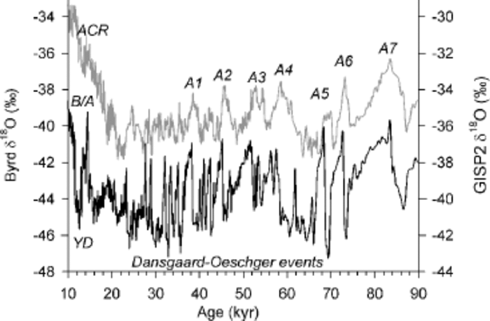
Fig. 1 Comparison of ice-core paleotemperature (δ¹⁸O) records from Greenland (GISP2, lower) and Antarctica (Byrd, upper), using the time-scales of Reference Blunier and Brook.Blunier and Brook (2001). ACR, YD and B/Arefer to the Antarctic Cold Reversal, Younger Dryas and Bølling/Allerød respectively.

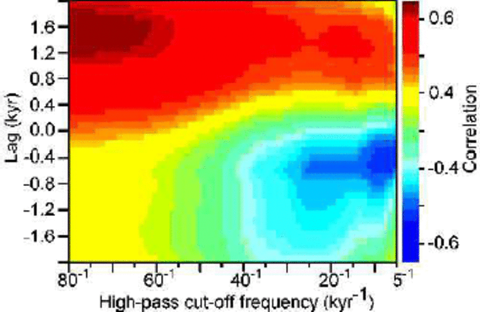
Fig. 2 Lag–correlation space for the Byrd and GISP2 δ¹⁸O records, showing correlation coefficients (colors) of high-pass filtered data as a function of high-pass cut-off frequency, 1/ 80 kyr^–1to 1/5 kyr^–A positive lag indicates a lag of GISP2 relative to Byrd.

As would be expected from previous work (e.g. Reference ImbrieImbrie and others, 1993), Figure 2 shows that secular variations, i.e. the lower frequencies associated with the ice-age cycles, are generally in phase in both hemispheres. This is indicated by the dominance of positive correlation coefficients (red and yellow) for cut-off frequencies <1/40 kyr^–1, with the highest correlation near lag 0. for higher frequencies, there are two maxima in the lag–correlation space. for the highest frequencies (cut-off >1/10 kyr^–1) the results show that a lead of Byrd over Greenland is statistically indistinguishable from a lag; either solution produces nearly equal maximum correlation coefficients. for positive lags, the maximum correlation is positive, indicating warming in Antarctica followed by warming in Greenland, consistent with the ``Southern lead’’ concept. the other correlation maximum is negative, a result consistent with the ``seesaw’’ model in which warming in Greenland is followed by cooling in Antarctica. the analysis thus illustrates what is readily apparent in a subjective analysis of the average relationship between the original time series: secular variations are generally in phase, while millennial-scale oscillations show both an approximate anti-phase and a phase-lagged appearance. It may be important that the lag at which maximum correlation occurs is greater for the Southern lead case (~1500 years) than for the Northern lead, anti-phase case (~400 years). It is also notable that very low correlation is obtained at zero lag. Because the maximum negative correlation occurs at about 400 years, which is somewhat larger than the relative dating uncertainty in the time series, it appears that a strict anti-phase relationship, as some descriptions of the seesaw model have implied (e.g. Reference White and Steig.White and Steig, 1998), is probably untenable.

Band-pass filtering and singular spectrum analysis

The high-pass filtering exercise described above, while removing low-frequency variations associated with orbital forcing, nevertheless retains multiple frequencies that may have independent physical significance. for example, Reference MayewskiMayewski and others (1997) attribute periods of 2.3 and 3.2 kyr in GISP2 chemical data to solar variability, while the ~1.5 kyr D-O period is attributed to an internal oscillation of the ocean thermohaline circulation. We therefore now seek to examine the phase relationships for individual frequency components. to do this, we employ both singular spectrum analysis (SSA) and band-pass filtering techniques. SSA provides a means to identify and selectively filter only the most important variations in the data, where ``importance’’ is defined in terms of the fraction of explained variance. SSA is mathematically equivalent to the ``empirical orthogonal function’’ eigenvector decomposition technique used in the analysis of meteorological data, but uses the covariance matrix of a single time series at various lags, rather than of multiple time series at different locations. We refer the reader to Reference GhilGhil and others (in press) for further details. for the bandpass analyses, we again use Butterworth filters designed with the Matlab^® ``filtfilt’’ algorithm.

SSA resolves the Byrd and GISP2 time series into five time principal components (PCs) that together account for >80% of the variance in each (lags up to 2 kyr were used in the calculation). Together, PCs 1 and 2 resolve the secular trends of the Milankovitch (orbital forcing) components of the data. PCs 3 and 4 of the GISP2 time series explain nearly identical fractions of the variance (9% each) and form an oscillatory pair that arises from a significant periodicity in the data (95% confidence against a red noise (AR1) process). Fourier analysis of the combined PCs 3 and 4 for GISP2 resolves a broad spectral peak covering periods of 4~–20 kyr, with a maximum at ~6 kyr years. Hence, the combination of PCs 3 and 4 is comparable to a broad band-pass filtered version of the original time series that excludes both low (orbital) frequencies and high (D-O) frequencies. SSA of the GISP2 data also reveals significant oscillatory components with maxima at periods of ~3.2 (PCs 5 and 6) and ~1.5 kyr (PCs 7 and 8), but these account for relatively small fractions (<5% each) of the variance. No periodic components in the Byrd data are identified by SSA, using the same criterion as for GISP2. These results are consistent with those of Reference Muller and MacDonaldMuller and MacDonald (2000), who note that the 1.5 kyr cycle exhibits significant spectral power only in part of marine oxygen isotope stage 3 (26–36kyr) in the Greenland data, and those of Reference Hinnov, Schulz and YiouHinnov and others (2002) who note that the 1.5 kyr cycle is very weak in the Antarctic data, even during stage 3. This may reflect the stronger expression of orbital components in Antarctic ice-core time series (for Byrd, PCs 1 and 2 alone account for >80% of the variance) or the more subdued nature of the Antarctic millennial-scale oscillations. Nevertheless, PCs 4 and 5 for Byrd together do form a weak (90% significance) oscillatory pair that has the same frequency maximum as the GISP2 PCs 3 and 4. Comparison between GISP2 PCs 3 and 4 and Byrd PCs 4 and 5 should therefore capture the dominant phase relationship (in the sense that it explains the largest fraction of the sub-orbital variance) between Antarctic and Greenland climate.

In Figure 3 are shown correlation coefficients for bandpass filtered components of the original data, calculated in 250 year steps with a 2 kyr bandwidth. Those frequencies identified as significant by SSA (6, 3.2 and 1.5 kyr periods) are denoted by dashed lines. Also shown for comparison are coefficients for the correlation of the PC pairs of GISP2 (3,4) and Byrd (4,5) identified with SSA. for each of these cases, the results compare favorably with those from the high-pass filter calculations: a lead of Byrd over Greenland (positive lag in Fig. 3) is statistically indistinguishable from a lag; either solution gives nearly equal maximum correlation coefficients. There is some variation, however, in the magnitude of the optimum lag; for the SSA PCs and the 6 kyr band-pass, maximum correlation is achieved for an Antarctic lead of ~1600 years and a Greenland lead (of opposite sign) of `800 years. These values are reduced to ~1500 and 600 years, respectively, for the 3.2 kyr band pass, and 1000 and 400 years for the 1.5 kyr period. Thus, the magnitude of the preferred lead–lag relationship is frequency-dependent, with climate events associated with longer-period variations having longer lead or lag times. This result is not an artifact of the smoothing of the time series that is inherent in the band-pass filtering process; the same result is also apparent in the high-pass filtering analysis, which retains the characteristic sawtooth pattern of the Greenland data.

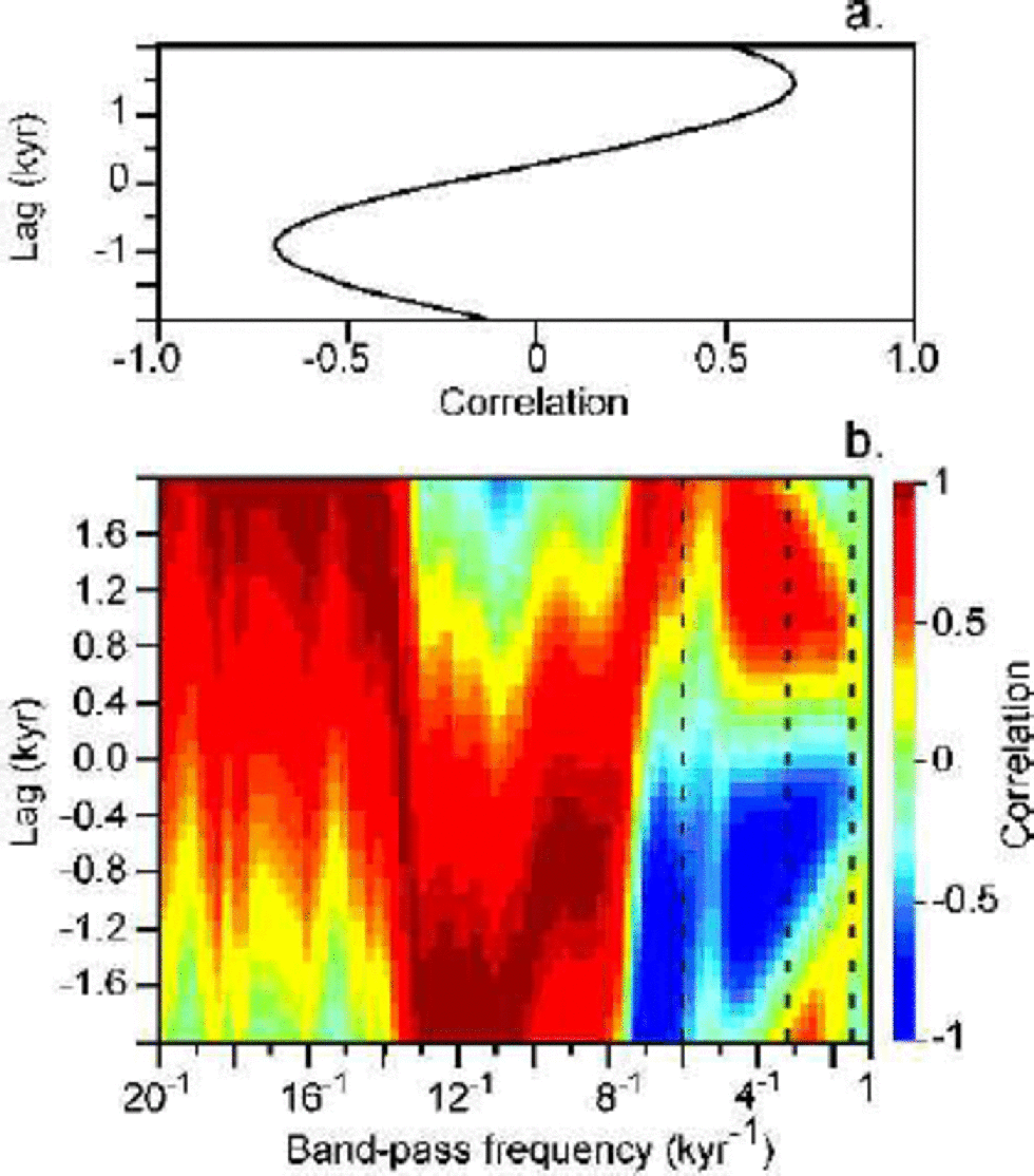
Fig. 3 (a) Correlation between combined PCs explaining the largest amount of millennial-scale variance in the GISP2 (PCs 3 and 4) and Byrd (PCs 4 and 5) data as a function of lag. (b) Lag–correlation space as in Figure 2, but using band-pass filters covering a period of 2 kyr and centered on the frequency shown. Dashed lines show frequencies of significant oscillatory components in the GISP2 data. A positive lag indicates a lag of GISP2 relative to Byrd.

Finally, we tested the robustness of all our results against possible bias that may have been introduced by including the entire time series from 10 to 90 kyr in our analysis. We repeated our analyses for the interval 26–36 kyr alone (this is the interval that shows the strongest 1.5 kyr periodicity), for the interval 36–60 kyr, and again for 60–90kyr. the results are essentially unchanged: in each case, the optimum correlation occurs at <1kyr for the GISP2-leading, antiphase case, and close to 1500 years for the Byrd-leading case. This is remarkable in that it shows essentially no time dependence to the results. This confirms the inference of Reference Blunier and Brook.Blunier and Brook (2001) that the same phase relationships apply to each of the rapid climate-change events, whether associated with short-duration D-O events, major A1–A4 interstadial events, or the even slower changes during the latter part of marine isotope stage 5. the frequency dependence noted above, however, does appear to be important, as it is maintained in each of these test cases, with the optimal lead of GISP2 over Byrd increasing from ~400 years for the 1.5 kyr band to ~800 years for the 6 kyr band.

Discussion

The analyses presented above indicate that from a statistical point of view, both the Southern lead (phase-lagged) and Northern lead seesaw (anti-phase) concepts are equally valid, if equally incomplete, descriptions of the Byrd and GISP2 time series. This is true in spite of the temptation to draw correlations between similar-looking features in the data, such as the rapid warmings in GISP2 and the long-term Antarctic warmings that seem to precede them. One might hypothesize, for example, that cooling at the beginning of the ACR in Antarctica ``caused’’ subsequent YD cooling in Greenland. An equally valid suggestion, however, would be that the gradual cooling in Greenland beginning at about 14 kyr, prior to the YD, caused the Antarctic warming that marks the end of the ACR. Although there may be other evidence that supports one hypothesis over the other, one cannot justifiably use the sign of the phase relationship as a diagnostic of the physical mechanism proposed. It is a given that any proposed physical mechanism for the causes of rapid climate-change events, and their linkage between the Northern and Southern Hemispheres, must produce phase relationships consistent with the observed data. However, we suggest that this is far from sufficient for model validation purposes. Possibly, the different lag times required for optimum correlation under a ``Greenland warming causes Antarctic cooling’’ scenario (400–800years), vs ``Antarctica leading’’ (1000–1600 years), could provide a useful model validation target. However, because the characteristic time-scale for ocean circulation between the hemispheres is of order 10³ years, it will prove difficult to rule out either scenario on this basis.

While our results suggest that there is no simple diagnostic phase relationship between the Greenland and Antarctic time series, the nature of the phasing may itself have physical significance in that it derives from the very different structures of the Antarctic and Greenland time series. the most obvious difference is that the rapid warming events in Greenland have no comparable analogs in Antarctica. Indeed, as Reference Hinnov, Schulz and YiouHinnov and others (2002) have pointed out, the lack of fast changes in the Antarctic records inevitably results in an average ``out-of-phase’’ relationship with Greenland, since Antarctica will almost always be changing gradually when Greenland is changing abruptly. Additionally, during many of the generally gradual cooling periods in Greenland, Antarctica is cooling rather than warming; that is, the two time series are generally in phase when both are changing gradually. This is not readily apparent for the YD/ACRtime period in a comparison of GISP2 and Byrd, but is quite obvious for the larger interstadial events. In other Antarctic ice cores, notably Dome C (Reference JouzelJouzel and others, 2001; Reference StenniStenni and others, 2001) and Taylor Dome (Reference SteigSteig and others, 1998, Reference Steig2000; Reference Grootes, Steig, Stuiver, Waddington, Morse and NadeauGrootes and others, 2001), the warmest temperatures of the last deglaciation occurred during the time of peak Bølling/Allerød warmth in Greenland, while the cooling that defines the beginning of the ACR parallels cooling in central Greenland towards the beginning of the YD. Thus, we suggest that the most important characteristics of the Greenland and Antarctic time series are the synchronous behavior during cooling and the fundamentally different (rapid vs gradual) behavior during warming. That such characteristics do, in fact, result in the apparent lag–lead relationships we observe in the data can be readily confirmed. We created a pair of synthetic, oscillatory time series that are precisely in phase during cooling, but that warm slowly in one case and rapidly in the other. As Figure 4 illustrates, these time series are, on average, ``out of phase’’ and their lag–correlation relationship is similar to that of the real GISP2 and Byrd time series. Inclusion of additional frequencies in the synthetic time series also reproduces the frequency dependence of the lag/lead times, as observed in the real climate data. We note that the recently published work of Reference Ganopolski and RahmstorfGanopolski and Rahmstorf (2001), which unlike most previous modeling work produces rapid warmings, rather than rapid coolings, in response to meltwater-forced thermohaline circulation changes, produces results quite similar to our Figure 4.

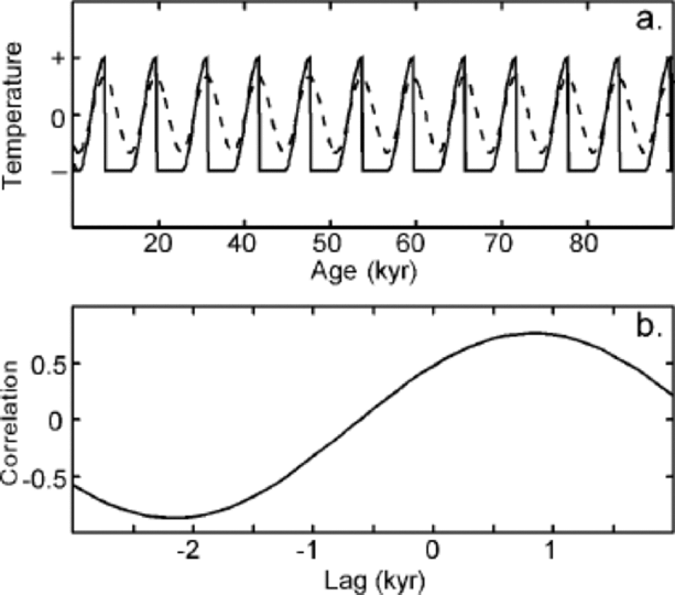
Fig. 4 (a) Synthetic Greenland (solid line) and Antarctic (dashed line) δ¹⁸O time series that are exactly in phase during cooling but where warming is abrupt only in Greenland. (b) Lag–correlation of these synthetic time series. A positive lag indicates a lag of Greenland relative to Antarctica.

Conclusions

We have presented several analyses showing that the simple relationships between Greenland and Antarctica climate implied by the concepts of anti-phase (``seesaw’’) or phase-shifted (``Southern lead’’) behavior do not adequately describe the real behavior of the climate system at millennial time-scales. Our results show that maximum positive correlation is achieved with a lead of the Byrd stable-isotope record over GISP2 of 1000–1600 years. Maximum negative correlation, with comparable significance, is achieved with an anti-phase relationship in which Byrd lags GISP2 by 400–800years. A strict anti-phase, however, is not supported by the data unless the relative dating is systematically in error by >400 years. the magnitude of the lags is frequency-dependent, with larger lags associated with lower-frequency climate changes. Because both an in-phase lead and an anti-phase lag of Antarctic vs Greenland climate are statistically similar, these characteristic phase relationships cannot be considered diagnostic of the location of origin (Southern Hemisphere vs Northern Hemisphere) of millennial-scale climate changes, nor of the physical mechanisms involved. Instead, these relationships do not imply any particular causal relationship, but arise from the fundamentally different nature of the climate time series. Most important is the presence of rapid warming events in Greenland in contrast with usually gradual warming in Antarctica. the relative rarity of rapid cooling events in Greenland, and the generally in-phase character of gradual cooling in both hemispheres, are probably equally critical. to be consistent with the observations, climate models will need to capture these aspects of the data in addition to reproducing the observed phase relationships. We do not propose a physical explanation here, but conclude that neither conventional ``Northern lead ’’models−with meltwater forcing in the North Atlantic being the dominant driving force for millennial-scale climate changes−nor alternative models with forcing from the Southern Hemisphere tropics or the Southern Ocean, can be ruled out on the basis of observed phase relationships between existing Antarctic and Greenland paleoclimate data.