


Introduction
Since the mid-1970s, there has been a great interest in developing hydro-power in Greenland. In 1982, the Geological Survey of Greenland (GGU) started a two-year glaciological programme in areas proposed for local hydro-power projects (Reference Weidick and ThomsenWeidick and Thomsen 1983b).
The work includes a basic inventory of hydrologic basins and glaciers, glacier mapping, collection of mass- balance and climatic data, and simulation of run-off, as well as glacier dynamics (Reference Braithwaite and ThomsenThomsen 1984).
A large part of the run-off from several basins under investigation is made up by melt water from the Inland Ice. The Inland Ice, covering about 79% of the total area of Greenland, represents a rather poorly-known area. Little information about topography, melt-water, and ice-flow patterns is available, due mainly to the size and inaccessibility of the ice sheet.
In several basins, lobes from the Inland Ice end up in the lakes proposed as reservoirs, or lie in between lake systems presently feeding the main reservoir. Glacier fluctuations can, in some cases, seriously influence the size of the reservoir and the direction of the melt-water drainage in the ice-free area.
Delineation of basins on the Inland Ice, related to water drainage, is difficult. The surface drainage pattern, inferred from maps, may not reflect the actual englacial or subglacial drainage pattern. Melt water may drain supraglacially, often through large river systems, directly to the glacier margin. However, much of the water reaches the bed through crevasses and moulins. Melt-water drainage, within and beneath glaciers, is very difficult to study and has mainly been dealt with through theoretical studies (Reference BjörnssonBjörnsson 1982; Reference ShreveShreve 1972; Reference WeertmanWeertman 1972), It is agreed that the subglacial topography can influence the direction of melt-water drainage, either by creating crevasses, affecting the surface drainage, or by forcing the water to follow subglacial valley systems.
Purpose of Glacier Mapping
The available maps covering the areas under investigation are the Danish Geodetic Institute standard maps on a scale of 1:250 000, with contour intervals of 50 m, and the ICAO World Aeronautical charts, on a scale of 1:1 000 000, with contour intervals of 300 m.
As pointed out by Reference Blachut and MüllerBlachut and Müller (1966), large- scale specialized maps are a prerequisite for most glacier investigations. In the present situation, detailed surface topographical data, data on subglacial topography, ice-flow and melt-water patterns were needed for large sectors of the Inland Ice. To meet these demands, a mapping programme was set up. Because of limited time, manpower, and financial resources for the project, the programme was designed to meet as many needs as possible and to produce data for planning of possible future work.
The most recent aerial photographs were used for photogrammetric plotting, to provide data on surface topography and glacier changes, but aerial photographs only exist for the outermost part of the Inland Ice. For coverage further inland, Landsat data were used for the extraction of information on melt-water and ice-flow patterns and for mapping the character of the subglacial topography as it is reflected on the ice surface.
Photogrammetric Mapping
margin of the Inland Ice and the adjoining ice-free area; north-east of Jakobshavn and north-east of Frederikshȧb, (Fig.1). The Jakobshavn map covers the area between 69° 20’N to 69°331N and 50°00’W to 50°27’W and includes the snouts and lower parts of six outlet glaciers (inventory nos. IGC0400I, 1GE0800I, 1GE07001 and 2, IGE04001 and 2). The Frederikshȧb map covers the area between 62° 11’N and 62°26’N and 48°52’W to 49°15’W and includes the snouts and lower parts of five outlet glaciers (inventory nos. 1BI0200I and 2, 1BI03001, 1BG03001 and 2).

Plotting was based on vertical aerial photographs from 26 June 1959, for the Jakobshavn area, and 2 July 1964. for the Frederikshȧb area. The photographs were taken from an altitude of 8860 m, at a photographic scale of 1:50 000, at a height of 1220 m. For plotting purposes, diapositives, provided by the Danish Geodetic Institute, were used. The map scale is 1:25 000, with contour intervals of 50 m in the ice-free area and 10 m on the ice. The maps were plotted at the GGU Photogrammetric Laboratory, using a Kern PG-2 stereo plotting instrument, connected to a computer system, First, aero-triangulation was made. Lakes and shorelines in the photographs were used to support the levelling of the models. For absolute orientation, control points were digitized from the Danish Geodetic Institute standard maps, as no ground control points exist in the area.
As pointed out by Reference SchyttSchytt (1966), the content of glacier maps depends on the nature of the study under consideration. In order to make the present maps widely useful, all possible glaciological and glacial geomorphological details have been plotted for the glacier area and trimline zone. On the Inland Ice, this includes debris-covered ice, streams, lakes, crevasses, and marked lineations. Within the trimline zone, moraines and the occurrence of glacial and fluvio-glacial deposits were plotted. This information is given by symbols in the geometrically correct positions. The symbols have been chosen to give as natural an appearance of the features as possible.
A section of the glacier map from the Jakobshavn area is given in Figure 2. The glacier maps from the Jakobshavn area and Frederikshȧb area are produced in full in Reference ThomsenThomsen (1983a) and Reference Weidick and ThomsenWeidick and Thomsen (1983a). For both areas, profiles have been plotted, giving the vertical height difference between the trimline zone, indicated by the top of exisiting lateral moraines, and the ice margin. The profiles have been placed where the ice margin is limited by steeper valley sides.
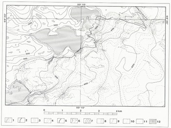
Fig. 2 Section of photogrammetric glacier map, showing a part of the Inland Ice margin in 1959 north-east ot Jakobshavn. Location is given in Figure 1.1) Contour on ice (10 m interval) 2) Ice margin. 3) Crevasses. 4) Lineation. 5) Debris-covered ice. 6) Stream (active, inactive). 7) Contour on land (50 m interval). 8) Trimline zone. 9) Moraines. 10) Glaciofluvial ridge 11) Glaciofluvial deposits. 12) Lake and fjord, with icebergs.
Satellite Mapping
Since the launching in 1972 of the first Landsat satellite, spaceborne remote sensing has been applied to the study of glaciers. Landsat images offer several advantages over other available methods for observing glaciers. In the case of the Inland Ice, a regional view is offered and a large part of the ice sheet, not covered by aerial photographs, can now be seen on one frame. Furthermore, Landsat data are available for times when aerial photographs are not usually taken,
Reference Krimmel and MeierKrimmel and Meir (1975) and Reference Thorarinsson, Sæmundsson and WilliamsThorarinsson and others (1973) show Landsat scenes, taken under conditions of low sun-angle, to be very suitable for accentuating subtle topographic surface features on glaciers, reflecting the subglacial topography.
For the purpose of this study, digital Landsat data (MSS), recorded late in the melt season, under low sun-angle conditions, were chosen. The data were analysed on the DK.IDIMS system (Danish Interactive Digital image Manipulation System) at the Technical University of Denmark. A description of the system is given in Reference Gudmandsen, Christensen and WolffGudmandsen and others (1982).
The first step in the image processing was a geometrical correction of the scenes. The corrections were carried out by a first-degree polynomial transform. The control points were taken from the Danish Geodetic Institute standard maps, on a scale of 1:250 000. This allows for a later inclusion of other map data, like terrain elevation etc. As ground control points, characteristic features on coastlines and river bends were chosen, for easy recognition in the near infrared band (band 7). The residuals in the transform fit were 0.66 pixel (52 m), as a mean. The resampling method was based on the grey-tone value of nearest neighbour pixel. Enhancement was used, to increase the contrast ratios in the image, so that individual surface features were more clearly differentiated. A linear stretch, based on the frequency distribution of the grey-tone values in the image, was applied. On the basis of the grey-level histograms, grey-levels representing the ice have been picked out and stretched over the total grey scale. Each band was stretched separately. Band 7 was assigned to the red gun, band 5 to the green gun, and band 4 to the blue gun, to form a false-colour image. False-colour images were taped and plotted on an Applicon ink plotter on a scale of 1:100 000. Ink plots, each covering about 54 x 79 km, were then “mosaiced”, to form Landsat image maps.
The Landsat image maps were used for interpretation and later plotting of surface features on the Inland Ice, to form surface feature maps. Experience through fieldwork on the Inland Ice, as well as vertical and oblique aerial photographs, was used to aid the interpretation of surface features. The Landsat image maps have a great ability to detect surface features related to ice flow, melt-water patterns and subglacial topography. Larger surface streams, medial moraines, and crevasse fields, related to ice streams and indicating the ice flow-patterns, are clearly depicted. Additionally, the character of the subglacial terrain is clearly depicted through shadow pattern, giving the ice surface a plastic appearance. On the surface feature maps, the individual features have been presented through a number of different signatures in the geometrically correct position. The subglacial terrain is represented through characteristic topographic features, such as valley limits, marked change in slope, and marked positive relief. In cases where the topographic relations are so complex that delineation of single elements was difficult, a signature for undulating terrain has been used. Correspondingly, marked linear structures represent linear elements, which are not possible to characterise topographically. The ice margin, lakes, and fjords have been delineated as given on the Danish Geodetic Institute maps. For final reproduction, the maps were photographed down to a scale of 1:250 00.
Surface feature maps have been produced for an area between 68°35’N to 70°00’N and 47°20’W to 50°30’W, east of Jakobshavn, and between 63°30’N to 64°36’N and 48 35’W to 50°05’W, in the Godthȧb area. (Fig.1). A section of the surface-feature map from the Godtháb area is shown in Fig.3. The maps are reproduced in full in Reference ThomsenThomsen (1983b).
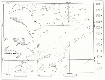
Fig. 3 Section of surface feature map, east of Godthâb. Location is given in Figure 1. 1) Lake and fjord. 2) Ice margin. 3) Stream on ice. 4) Nunatak. 5) Medial moraine. 6) Flowlines. 7) Major crevasse field. 8) Valley limits (certain, uncertain). 9) Marked change in slope. 10) Marked positive relief. 11) Undulating terrain. 12) Marked linear structure.
Some Results and Use of Glacier Mapping
The glacier maps have been used for estimating the size of drainage basins on the Inland Ice, related to ice flow and melt-water drainage, to provide data for runoff simulations (Reference Braithwaite and ThomsenBraithwaite and Thomsen, 1984) and simulation of glacier dynamics (Reference ReehReeh, 1983).
For the delineation of hydrologic basins, the character of the subglacial terrain was taken into acount, as it is assumed to affect the drainage pattern. The areas proposed for hydro-electric installations are located along relatively quiet sectors of the Inland Ice, ending up in larger lakes at high elevation, to be used as reservoirs. These sectors are separated by more active sectors, feeding large outlet glaciers reaching sea level. Estimates of the size of hydrologic basins on the ice show that smaller areas than estimated earlier can be expected. This is mainly due to active ice drainage to the large neighbouring outlet glaciers, ending up at sea level, and to the existence of distinct, subglacial, topographic features, which must be assumed to influence the direction of melt-water drainage. Run-off simulations based on these revised area estimates, are in better agreement with measured run-off from the areas than was found earlier.
More exact data on the subglacial topography are necessary for further model simulations. For this purpose, radio echo-sounding has been started (Reference Thomsen and MadsenThomsen and Madsen, 1985). In this connection, the glacier maps serve as an important basis for location of study areas and for planning tracks of radio echo-sounding.
Acknowledgements
This paper is published with the permission of the Director, The Geological Survey of Greenland. The project was supported by EEC’s European Fund for Regional Development. Thanks are due to Bruno Wolff (DK. IDIMS) and the entire IDIMS users group, Technical University of Denmark for making the work there a pleasure. I thank Olav Winding (GGU) and Hans Jepsen (GGU) for useful discussions and help with the photogrammetric work.


