


Introduction
A survey network of more than 200 aluminium poles on Rutford Ice Stream (Fig. 1) has been described and preliminary results have been presented (Reference Stephenson and DoakeStephenson and Doake 1982,Reference Doake, Frolich, Mantripp, Smith and Vaughan Doake and others 1987, Reference Frolich, Mantripp, Vaughan and DoakeFrolich and others 1987). A longitudinal stress-gradient equation has been used to partition the resistive forces between marginal (side-wall) shear, basal friction and localized bending (Frolich and others 1987), in an attempt to understand the processes opposing the gravitational driving force. A 60 km longitudinal line of the network (Fig. 2) has been treated for its force balance in this way. The horizontal shear stresses generated by contact with rock and slower-moving ice at the glacier margins were represented by yield stresses of 100 kPa acting at these margins, with a constant transverse gradient of shear stress between them. The subsequent analysis of transverse profiles on the network, at each end of the 60 km longitudinal line, together with results from the down-stream transverse line (Fig. 2), has allowed this approximation to be discarded and a more confident assessment to be made of where the major restraint occurs.

Fig. 1. Location of Rutford Ice Stream.

Fig. 2. Full stake network superimposed on a Landsat image of Rutford Ice Stream (courtesy of Dr Β. Lucchitta, U.S.G.S., Flagstaff, AZ 86001, U.S.A.). The position of the longitudinal network discussed in this paper lies between A and C, crossing a prominent surface knoll at B. The direction of ice flow is from left to right, the Ellsworth Mountains are at the bottom of the image and Fletcher Promontory is at the top.
Data Acquisition and Analysis
The data were obtained from conventional survey techniques and radar sounding. Survey control was provided by Magnavox MX1502B doppler satellite receivers, using the Transit system. Collection of the data is described in more detail in Doake and others (1987) and Frolich and others (1987). Stations were arranged in double lines, with typical separations of 2-3 km. Positions and velocities for the stations were obtained from the solution of time-dependent observation equations (Reference Wager, Doake, Paren and WaltonWager and others 1980), and the residuals were used to estimate uncertainties in the solutions and in the strain-rates derived from them. Random errors in observation typically contribute an error of about 10−4a−1in magnitude and 1° in orientation of the principal axes of strain-rate. Surface velocity, surface elevation andice thickness are treated as varying linearly over each triangle of adjacent stations, with average values and gradients applying at the centroids. Stations were generally surveyed twice, with an interval of about 1 year. Any redundancy is used for checking and estimating uncertainties, so values for gradients in strain-rates in both directions normally exist only at the intersections of the longitudinal line with transverse lines.
The longitudinal stress-gradient equation used is similar to that given by Frolich and others (1987), with the exception that the three components of the force acting at the base have been separated, giving

where the stresses normal and tangential to the upper surface have been taken to be zero (x- and y-axes are horizontal, with x positive down-stream; the z-axis is vertical, positive upwards with surface at z s and base at z b; Η is the ice thickness, ρ is the mean ice density, and g is the gravitational acceleration). This equation can be shown to be equivalent both to the form obtained by Reference CollinsCollins (1968) in the case of vanishing transverse gradients and to similar formulations due toReference Robin.de Robin (1967), Reference NyeNye (1969), Reference BuddBudd (1970),Reference HutterHutter (1983),Reference MacAyeal, Shabtaie, Bentley and King MacAyeal and others (1986),Reference Morland, Veen van der and Oerlemans Morland (1987) and Reference Whillans and van der VeenWhillans and van der Veen (1988, this volume). The last term in Equation (1) is often known as the “T” term (Nye 1969). A similar equation exists for theother horizontal direction, but we do not have values for second spatial derivatives of velocity over a wide area which would enable an arbitrary path of integration to be taken. The Α-coordinate has therefore been taken to agree closely with the line of the network and the mean flow direction. Equation (1) thus represents a force balance per unit width integrated along an approximate flow line between a point x' and a down-stream limit L. For the calculation of stresses from field data, an effective viscosity v was defined, using a flow law of the form
where σ′ ij is the stress deviator,
is the strain-rate,
is the second invariant of the strain-rate tensor, and B is a temperature-dependent parameter whose mean value was taken to be 4 × 10⁵Pa a1/3 for n = 3. Although the index n is usually assumed to be 3, implying non-linear flow, there is some doubt about experimental evidence from the field for this value, and a linear viscosity where n = 1 may be equally applicable (Reference Doake and WolffDoake and Wolff 1985, Reference PatersonPaterson 1985, Reference Wolff and DoakeWolff and Doake 1986). Only the strain-rates measured at the surface were available for the calculation of values for Ė, and incompressible flow was assumed. If vertical shear is significant, then the calculated effective viscosities will be too high and the stresses will be overestimated. As no information on variations in parameters with depth is available, integrals overdepth have been approximated by assuming that the strain-rates are independent of depth, as would be expected in an iceshelf. The validity of this assumption is discussed later.
The force balance may be written in symbolic form
where V is the viscous response, DF is the difference in driving force between x′ and L, and RF is the difference in restraining force between x′ and L (the sum of the last three integrals in Equation (1)). The variation in these terms along the longitudinal line is shown in Figure 3.

Fig. 3. Terms in the force-balance equation for the longitudinal line between A and C in Figure 2. The symbolic names are explained in the text (RF is the restraint, V is the viscous response, DF is the driving force).
Discussion
Elevation and velocity profiles for the three transverse lines are shown in Figures 4 and 5. The two lower lines ((b) and (c)) cover the central part of the ice stream and do not penetrate the marginal zones to any significant extent. The up-stream line (a), however, crosses the boundary on to Fletcher Promontory, where there appears to be a small component of flow in the direction opposite to that of the ice stream, due to ice discharging from the prominent cirque. In the main body of the ice stream the greatest variation in ice thickness occurs in the middle transverse profile (b), where there is a relief of around 500 m in the subglacialtopography. The longitudinal stake line crosses this transverse profile near the crest, which appears to be a continuation of the bedrock step, manifested on the surface by a knoll found farther up-stream (Frolich and others 1987).

Fig. 4. Surface-elevation and bed profiles for the three lower (down-stream) transverse lines shown in Figure 2 ((a) isthe middle line, (c) is the line farthest down-stream). Arrows indicate the approximate location of the longitudinal line.

Fig. 5. Fig. 5. Velocity profiles for the three lower (down-stream) transverse lines shown in Figure 2 ((a) is the middle line,(c) is the line farthest down-stream). The direction of the horizontal velocity is along a bearing of 160° true. Arrows indicate the approximate location of the longitudinal line.
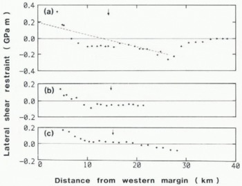
Fig. 6. Fig. 6. Profiles of lateral shear stress integrated over depth for the three lower (down-stream) transverse lines shownin Figure 2 ((a) is the middle line, (c) is the line farthest down-stream). The dotted line shows a constant shear-stress gradient which assumes a shear stress of 100 kPa at each margin. Arrows indicate the approximate location of the longitudinal line.
The thickest ice and deepest glacial bed lie on the western side of the ice stream, close to the Ellsworth Mountains. The maximum forward velocity is also displaced towards this side. Horizontal shear strain-rates
for the upper two transverse lines pass through zero at the same position as the maximum value of the velocity,as expected. The surface strain-rates have been converted to depth-integrated shear stresses, shown in Figure 6, by the formula

The parameters n and Β in the flow law are assumed to be constant across a profile, and the depth-averaged value of
is assumed to bear a constant relationship to the surface value, i.e.
where β is independent of y. The restraint from side-wall (marginal) shear (SW) arises from the gradient of the shear stress in the y-direction:

so a value of β constant with y will be equivalent to a scale change in the magnitude of the shear-restraint profiles shown in Figure 6. These profiles do not have a constant slope, as would be expected if side-wall shear extended its influence uniformly across the glacier and as is frequently assumed to be the case for ice shelves (Reference ThomasThomas 1973). Instead, a boundary layer about 10 km wide on the western margin experiences a high gradient and is followed by a central region where the gradients are very small and not significantly different from zero. The gradients increase again in the eastern margin.
The highest calculated horizontal shear stress, at the western margin of the upper line, is about 160 kPa. Such a high value suggests that the effective viscosity may have been overestimated, due in part to assuming that it is constant with depth, whereas warmer deeper ice should be softer than ice at the surface. The ice at the western margin will generally have come from steep valley glaciers in the Ellsworth Mountains and have a complicated stress history. Its incorporation into the boundary may therefore result in anisotropies in the fabric and a more easily deformed layer. This couldalso apply at the eastern margin, because ice floating slowly off Fletcher Promontory forms a boundary layer. MacAyeal and others (1986) suggested that the boundary between fast-flowing ice shelf and land-fast ice may be weakened by faulting and they described the boundary in terms of a coulomb rheology. This may be equally applicable in the case of ice streams. Alternatively, strain heating in regions of high shear or inadequacies in the flow law may both be important.
It seems likely, however, that the ice rheology changes little across the middle third of the ice stream, and that the flatness of the lateral shear profiles reflects a lack of restraint from the margins. This leaves only forces at the base and the “Τ” term to balance the variations in driving force. The “T” term is frequently assumed to average to zero over distances of more than a few ice thicknesses (Reference Kamb and EchelmeyerKamb and Echelmeyer 1986). If this is indeed the case, then forces acting at the base must account for almost the entire variation in restraining force (RF) along the network (Fig. 3).
This is a surprising result in view of the high surface velocities and the possibility that the basal ice is at its pressure-melting point. The longitudinal average value of the driving stress is about 40 kPa, which must be balanced by a basal shear stress of about the same magnitude. Taking the calculated values of effective viscosity and assuming that the variation in the vertical shear stress (σ xy ) is linear with depth, then a basal shear stress of 40kPa would give a difference between surface and basal velocities of the order of 10 m a−1 (the measured surface velocity varies from about 360 m a−1 to 400 m a−1 along the longitudinal line). This difference is probably too small to be detectable from the surface, either with radar-fading patterns (Reference DoakeDoake 1975) or from mass-flux calculations, suggesting that direct observations at depth may be required.
The third transverse profile (Fig. 6(c)) lies down-stream of sites where tidal flexure has been observed (Reference StephensonStephenson 1984) and may be entirely on floating ice. A difference in gradient between the western margin and central regions of theice stream is still apparent, though less distinctly than on the other two profiles. The contribution of lateral shear to the restraining force must therefore still be small, but in this case the much smaller surface slopes mean that the driving force which must be balanced is also small. The ice stream is in longitudinal compression here (Stephenson and Doake 1982), further reducing the restraint necessary for balance.
Although the variation in stresses with depth has not been treated rigorously here, the conclusion that marginal shear is unimportant near the centre of the ice stream suggests that a two-dimensional simplification may be made that would allow a self-consistent solution for the distribution of basal and vertical shear stress (σ xz ). Figure 3 shows that the viscous terms (the one on the left-hand side of Equation (1) and the first term on the right-hand side) containing the direct stresses are much smaller than either the driving force DF or the restraining forces RF. Therefore, not knowing the variation in
or
with depth should not lead to large errors when calculating RF. By ignoring gradients in the y-direction in the RF terms in
Equation (1), and neglecting

In conclusion, it appears that in this part of Rutford Ice Stream there are two distinct flow regimes: a marginal zone in which side-wall shear is important, and a central region where basal friction dominates. The transition from ice-sheet to ice-shelf-type flow probab]y occurs in a non-uniform manner, in which several different processes interpenetrate along the ice stream and are responsible for the overall force balance.


