


1. Introduction
Surface melting occurs during summer on some low-lying regions of the Antarctic ice sheet. Melting takes place mainly in the blue-ice areas of the glacier—ice-shelf systems, where the surface albedo is low, and to a lesser extent in the snow-covered accumulai ion zones if air temperatures are high enough. Mcltwater produced is transported northwards in meltwater runoff streams (Reference Winther, Elvehøy, Bøggild, Sand and ListonWinther and others, 1996; hereafter referred to as meltstreams), and collects in surface hollows forming meltwater lakes, a process known as ponding. Meltstreams lead to a redistribution of mass within a glacier-icc-shelf system and a loss of mass if they reach the ice front or penetrate the ice shelf at moulins. There are large annual variations in the meltstream intensity, spatial distribution, onset time and duration (Winther and others, 1996); monitoring these features could provide a sensitive indicator of regional climatic variability.
This paper uses a synthesis of remotely sensed and field data to investigate a meltstream on the Amery Ice Shelf. Re-frozen meltstreams are observed in a surface map produced from the Amery Ice Shelf GPS survey (1995) and in a synthetic aperture radar (SAR) image. Using two further types of microwave remote-sensing instruments, the radar altimeter (RA) on the European remote-sensing satellite ERS-1, and the special sensor microwavc/imager (SSM/I) on the Defense Meteorological Satellite Program (DMSP) satellite, the development of the meltstream during the 1993-94 summer is monitored.
2. Surface Meltstreams on the Amery Ice Shelf
2.1 Previous observations (1960-90)
Mellor and McKinnon (1960) were the first to document surface melt features in the Lambert Glacier-Amery Ice Shelf (LG-AIS) system.The.se perennial features have subsequently been detected by aerial observation during Australian National Antarctic Research Expeditions (ANARE) in 1988-90 (personal communication from I. Allison, 1996) and in Landsat satellite imagery (Reference SwithinbankSwithinbank, 1988). Observations from snow pits and shallow cores also show evidence of meltstreams in superimposed ice layers, interspersed with layers of winter snow accumulation (Reference Landon-SmithLandon-Smith, 1962; Reference GoodwinGoodwin, 1995).

Fig. 1. Location map of the Amery Ice Shelf, showing the GPS survey grid, ERS-1 ground tracks and the three SSM/I polygons (North, Central and South). The ERS-1 3 day repeat track and the five 168 day tracks (four ascending, one descending) are shown as a solid line and dashed lines, respectively. Arrows on these tracks indicate the direction of satellite travel.
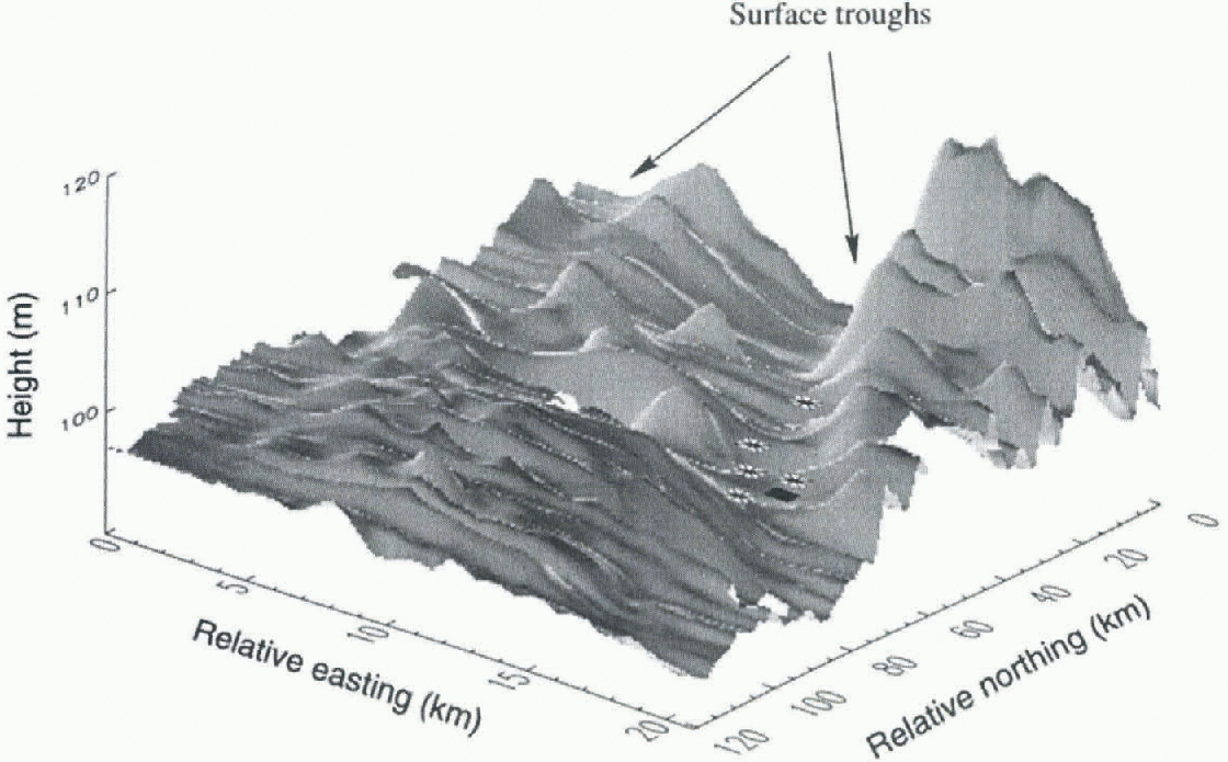
Fig. 2. Shaded ice surface generaled from the GPS survey data, on a 0.5 km grid using kriging. Units of the horizontal axes are kilometres, with the origin in the southeast corner. Units of the vertical axis are metres, therefore the plot is exaggerated in this direction. The diamond and asterisks represent the locations of the backscatler peak and central specular return for the 3 and 168 day repeat data, respectively.
2.2. Recent observations (1993-95)
The Amery Ice Shelf mapping programme took place between 25 October and 14 November 1995, before the 1995-96 summer melting. A 120 km by 20 km grid made up of 24 10 km squares was surveyed using kinematic global positioning system (GPS) techniques. The orientation of the grid on the ice shelf is shown in Figure 1, together with the ground tracks of the ERS-1 orbits which cross it (discussed laler). Six base camps were established along the centre line of the grid at 20 km spacing.
A surface elevation model for the survey region, created from the kinematic GPS profiles using “kriging” (Reference CressieCressie, 1993), is shown in Figure 2. The model reveals two longitudinal shallow troughs, approximately 3 km wide, 5 m deep and more than 60 km long. During the 1995 Amery survey, pit measurements at a camp located in one of the troughs revealed one layer of snow (27 cm deep) on top of hard, bubble-free ice. This, combined with the fact that the troughs are flat-boltomed, suggests that they once held water that has since refrozen.
Meltstreams on the Amery Ice Shelf are also evident in recent SAR imagery. Figure 3 presents an ERS-1 SAR image acquired on 15 August 1993, warped onto a polar Stereographic projection, with the GPS survey grid (shown in Fig. 1) and the ERS-1 3 day track overlaid. The prominent dark features with in the grid are refrozen meltstreams, standing out clearly from the surrounding ice shelf due to their different near-surface properties and low surface roughness. The location of the refrozen meltstreams matches well with the troughs seen in Figure 2.

Fig. 3. SAR image over the Amery Ice Shelf, with GPS survey grid, ERS-1 altimeter and 3 day repeat (track 013). The white square denotes the location of the backscatler peak and main specular return from the track 013 repeats.

Fig. 4. (a) Selected ERS-l waveforms along track 013 over the central Amery Ice Shelf on 27 January and 2 February 1994. The vertical scale is an arbitrary measure of power, (b) Time series of altimeter waveforms from the centre of the surface trough, for all ice-mode repeals along track 013. The vertical scale is an arbitrary measure of power.
3. Detection of a 1993-94 Meltstream with ERS-1 Radar Altimetry
3.1. The ERS-1 radar altimeter
The ERS-1 altimeter obtains the range from the satellite to the Earth's surface by measuring the travel time of a radar pulse. The return signal is not continuously recorded, but is digitised during a small range window, which is positioned by the on-board tracker (Guskowska and others, 1990).The form of the returned signal within this range window depends on the geometry and electromagnetic scattering properties of the surface. Over most of an ice shelf altimeter waveforms are simple, being returns from a flat surface, with scattering primarily from the surface alone (Reference Ridley, Cudlip, McIntyre and RapleyRidley and others, 1989).
Another measurement made by the ERS-1 altimeter is the microwave backscatler (σ°), i.e. the intensity of the signal reflected by the surface received back at the radar. Variations in σ° arise due to changes in surface properties (e.g. moisture content and surface roughness).
The ERS-1 satellite has operated in orbits with repeat periods of 3, 35 and 168 days. Data used in this study are from a 3 day and a 168 day phase. The 3 day phase (23 December 1993-10 April 1994) had a wide ground-track spacing of ~300 km at 71° S. Only one of these tracks, shown as a solid line in Figure 1, crosses the Amery Ice Shelf. in the 168 day phase (10 April-27 September 1994), the long repeat period meant that the tracks were more closely spaced (~2.5km at 71°S) but the time interval between measurements with in the same neighbourhood was long. The five 168 day orbits used in this analysis are shown as dashed lines in Figure 1. The ERS-1 altimeter has two modes of operation: ocean and ice. Over the Antarctic ice sheet it was alter-nated between ocean and ice mode during the 3 day phase and was always in ice mode during the 168 day phase.
3.2 ERS-1 altimeter waveforms
figure 4a presents sequential altimeter waveforms along track 013 over the survey region, for adjacent ice-mode repeats (27 January and 2 February 1994). The waveforms are approximately aligned by position: i.e. waveforms with the same number from each sequence are from similar locations along track.
In the sequence from 27 January, waveform 1 is a typical ice-shelf return, with a well-defined leading edge (A). The bump (B) at the back of waveform 2 occurs because the altimeter views two surfaces at different ranges, indicating that a new, lower elevation surface is entering into its footprint. in waveform 3 the higher surface has retreated and the sharp leading edge indicates that the low surface has become dominant; the satellite is directly above the surface trough. Waveform 4 shows the altimeter leaving the trough and moving back onto the main ice shelf, and waveform 5 is once again a fairly typical ice-shelf return.
The sequence from 2 February is similar, except in the centre of the trough (waveform 3) where the waveform is narrow-peaked. This waveform has a very steep leading edge and large amplitude (the power scale has been multiplied by a factor of 10), and is termed quasi-specular (Reference Rapley, Guzkowska, Cudlip and MasonRapley and others, 1987). The position of this return is illustrated as a black diamond in Figure 2 and a white square in Figure 3.
figure 4b illustrates the evolution with time of the approximately central waveform, for the 12 ice-mode re-peats from 27 January. The shape remains quasi-specular for two repeats and displays a sharp peak until 9 April. Specular waveforms are also present in five orbits of the 168 day phase which cross the survey region (plotled in Fig. 1). The locations of the main specular return for these orbits are plotted as black asterisks in Figure 2; these points also lie in the surface trough. These orbits are from 29 April, 16 May, 5 June, 11 June and 12 July.
3.3 ERS-1 measured backscatter (σ°)
figure 5a illustrates the microwave backscatter (σ°) measured along track 013 across the Amery Ice Shelf for the (wo repeats shown in figure 3a. There is a large increase (about 20 dB) in σ° on 30 January 1994, which coincides in position with the central quasi-specular waveform (waveform 3 in fig. 4a).
figure 5b shows the change in the value of the σ° peak for all of the ice-mode repeats along track 013 (25 Decem-bei—9 April). σ° remains fairly high for a period of about a week, but decays after its peak value on 2 February. The backscatter drops to around 16 dB, and remains fairly constant through to the end of April.
4. Supporting Evidence of 1993-94 Summer Melting
4.1 SSM/I brightness temperatures
The SSM/I, on board the DMSP platform, is a passive microwave sensor that measures surface brightness tem-peratures. The brightness temperature (T b) of an object is a measure of the intensity of the microwave radiation it emits. It is the product of the object's absolute physical temperature and its emissivity. The emissivity is dependent on the object's physical properties. For snow it increases with moisture content and as grain-sizes decrease (Reference Zwally and GloersenZwally and Glocrsen, 1977). Surface melting increases the moisture content of the snow, increasing its emissivity and Tb . Large increases in T b during the summer months indicate the onset of melting (Ridley, 1993).

Fig. 5. (a) ERS-1 measured backscatter along track 013 across the central Amery Ice Shelf on 27 January and 2 February 1994. ( b) Time series of maximum backscatterfor all ice-mode repeats along track 013.
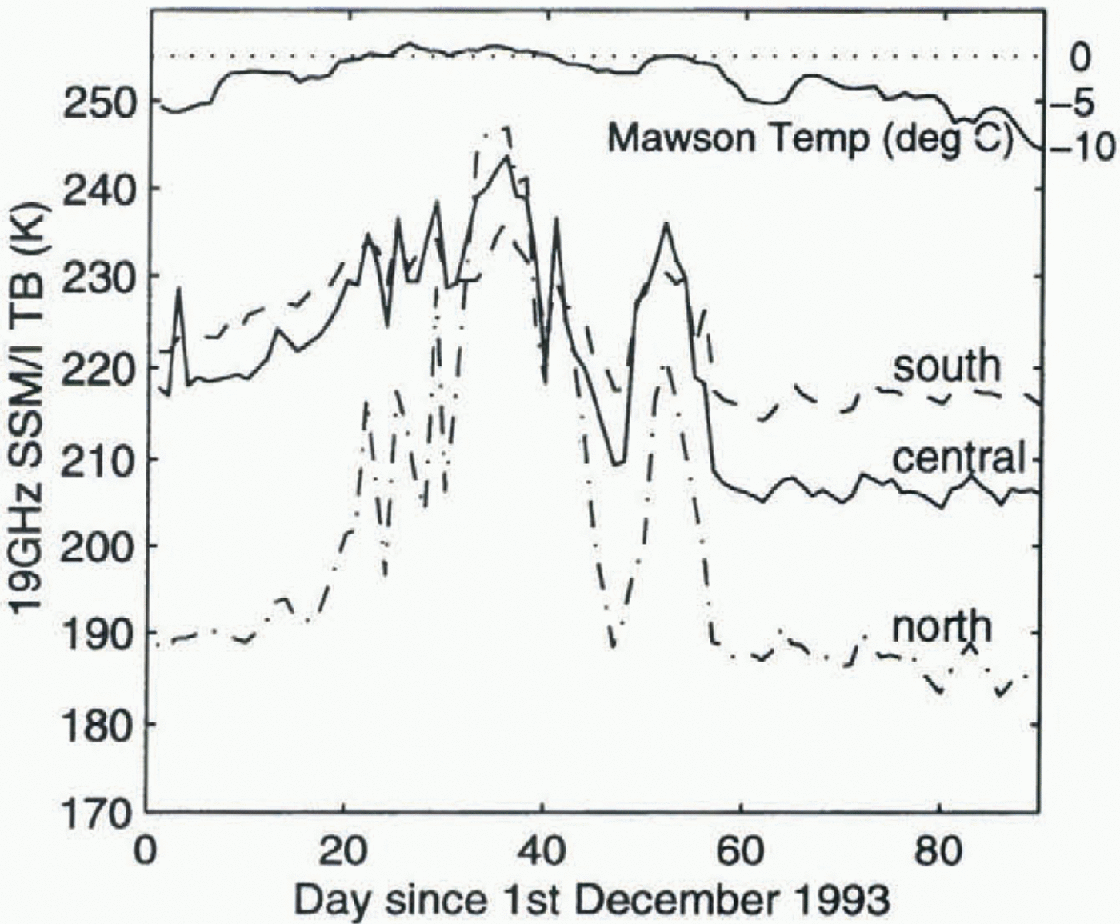
Fig. 6. Time series of daily SSM/1-derived passive-intero-wave brightness temperatures averaged over the three polygons in the LG—AIS system illustrated in Figure 1. The top line is the average daily temperature at Mawson station.
To determine when melting occurred in the LG-AIS system during the 1993-94 summer, average daily Th values were calculated over the three large polygons in the region, shown in Figure 1. The three time series of average 19 GHz (vertical polarisation) T b values are shown in Figure 6. Values decrease from south to north because grain-sizes increase in this direction (Zwally and Fiegles, 1994), reducing the emissivity. The T b values increase slowly with temperature from 1 December until the first melting event in late December, when they increase rapidly to approximately 240 Κ over all three regions. The peak occurs around 5 January (day 35), corresponding to full saturation of the snow. The values then decrease steadily, until around 21 January (day 51) when there is a secondary rapid increase.
4.2 Temperature data
The top line in Figure 6 is the average daily temperature at Mawson station, ~300 km northwest of the SSM/I polygons. The periods of summer melting observed in the SSM/I T b values coincide with the periods when the temperatures at Mawson were 0°G or above.
5. Discussion
The observed increase in ERS-1 measured microwave back-scatter (σ°) on the Amery Ice Shelf on 30 January, combined with the sudden transition to a quasi-specular return, indicates that there must be a rapid change in surface properties taking place at this time. Such a dramatic signal can be explained by the arrival of free-standing water in the altimeter footprint, causing strong reflections of the radar pulse. Melting events are observed in the SSM/I time scries on 5 and 21 January 1994. It is thought that these melt events triggered a large meltstream, explaining the presence of water in the altimeter footprint several days later.
The ERS-1 altimeter has a surface footprint with diameter 6-8 km over the Amery Ice Shelf; the smooth surface of the meltstream therefore lies with in the footprint before the satellite is directly overhead, and after it has passed. The parabolic shape of the a° variation observed in figure 6a indicates that the reflecting area is small. The position of the parabola peak coincides with the position of the centre of the surface trough mapped with GPS in Figure 2.
The drop in the maximum σ° value after 27 January occurs because the water in the surface meltstream refreezes as air temperatures decrease. On refreezing, the surface remains “smooth”, therefore the waveforms continue to be quasi-specular. However, the lower reflectivity of ice compared to water, combined with the fact that surface roughness increases after refreezing due to the formation ot microcracks in the surface, leads to the observed drop in σ°.
One of the 168 day orbits crossed the Amery Ice Shelf very close to track 013 on 5 June. This orbit contained specular waveforms and still had a peak σ° value of 15.3 dB over the melt channel. This suggests there was little change in surface properties between late February and earlyjune. in fact, backscatter peaks and specular returns persisted until 12 July in the 168 day profiles. It seems therefore that the surface remained fairly smooth throughout this period and that there was no, or very little, snow build-up on top of the ice until after 12 July. The addition of a layer of snow would increase the surface roughness and therefore reduce the backscatter; addition of more snow layers would eventually lead to the removal of the backscatter peaks and quasi-specular returns. That is, the surface characteristics would return to the pre-meltwatcr state observed from December to January. Monitoring the persistence of the backscatter peaks and the specular returns over meltstreams could be one indicator of variations in regional snow accumulation.
The SAR image in Figure 3 shows that the eastern, shallower trough was also occupied by meltwater in the pre-vious year (1992-93). However, from the results of the altimeter analysis it does not appear that this trough carried water during 1993-94. Ablation rates on the Amery Ice Shelf, estimated from temperatures at Mawson, indicate that there was less meltwater in 1993-94 than in 1992-93, therefore it only occupied the main trough that summer.
6. Conclusions
The presence of standing water with in the ERS-1 altimeter footprint leads to a quasi-specular return and high back-scatter values. The standing water detected in the ERS-1 data during the 1993 94 summer arose from meltwater which flowed slowly along gently sloping surface troughs observed in the GPS surface and a recent SAR image. There was a time delay of about 25 days between the onset of melt in the LG-AIS system and the arrival of meltwater on the accumulation region of the Amery Ice Shelf. The backscatter remained high, at a value of above 30 dB, for approximately a week before dropping to 15 dB as the water froze. Specular waveforms and a peak backscatter value of 15 dB remained until 12 July, suggesting that the surface was still bare ice with little snow accumulation.
A consequence for satellite altimetry over ice shelves when meltstreams are present is that the altimeter will range to such features for as long as they remain in its fool-print, a problem known as “snagging". The resulting specular waveform will be at the correct position with in the range window only when the meltstream is directly at nadir. The remaining overestimated range measurements should be removed from any altimeter dataset, as they result in surface elevations that are too low. Waveforms of this type persisted in ERS-1 satellite altimeter data from 1994 over the Amery Ice Shelf for more than 5 months (2 February 12 July).
This paper has presented a comprehensive analysis of several methods for detecting surface meltstreams, and outlined a simple, robust technique for monitoring the onset and duration of meltstreams using high-temporal-rcsolution RA data. The location of the ERS-1 3 day track on the Amery Ice Shelf was fortuitous; unfortunately, the poor spallai coverage limits the possibility of similar studies over other regions of Antarctica where surface melting and runoff occurs. Knowledge of the time of arrival of meltwater in the channels could be used in combination with other remote-sensing techniques to interpret images (if available) from the same time (e.g. SAR, Landsat). Changes in the distribution of melt and redistribution of meltwater could provide validation for or assessment of regional climatic change. Knowledge of positions of meltstreams could also improve models of the regional surface mass balance of the Amery Ice Shelf.
Acknowledgements
The author would like to thank J. Ridley, I. Allison, N. Young and R. Coleman for their useful input into this paper. Grateful thanks also to G. Hyland for help with data processing, and to all the members of the .WARE Amery Ice Shelf 1995 field survey. The ERS SAR and RA data were supplied by the European Space Agency (ESA) through the ERS Announcement of Opportunity Project ERS.A02.AUS103 ¡principal investigator N.Young). All ERS data are copyright to ESA, 1993 and 1994.


