


Introduction
Deep ice-core drilling operations require that the borehole be filled with a fluid to compensate the ice pressure at great depth (Talalay, Reference Talalay and Gundestrup2002a, Reference Talalay and Gundestrupb). The drilling fluid used for recent European drilling projects such as the North Greenland Icecore Project (NorthGRIP; Reference Dahl-JensenDahl-Jensen and others, 2002), the European Project for Ice Coring in Antarctica (EPICA) Dome C (Reference Augustin and AntonelliAugustin and Antonelli, 2002), Berkner Island, Antarctica, (Reference Mulvaney, Alemany and PossentiMulvaney and others, 2008) or Talos Dome, Antarctica, (Reference SalaSala and others, 2008) is mainly a mixture of a petroleum oil product, similar to kerosene (with a density of 800–850 kgm–3 at –30˚C), with dichlorofluoroethane HCFC-141b (with a density of 1325 kgm–3 at –30˚C) added to increase the density to as close as possible to the mean ice density. Although these binary drilling fluids have already been described (Reference Talalay and GundestrupTalalay and Gundestrup, 1999, 2002a, b), there is still much to learn about the properties of the mixture of drilling fluid and ice chips.
The drilling-fluid/ice-chips mixture has been considered as a homogeneous fluid with mean physical properties that correctly characterize the real solid/liquid suspension. To extend this to a hydraulic calculation for the lower part of a drill requires knowledge of the two main fluid parameters: (1) the fluid density and (2) the fluid viscosity.
The goal of this paper is to propose a method to calculate, to a first approximation, both these parameters. The drilling fluid chosen in the experiments performed in cold rooms at Laboratoire de Glaciologie et Géophysique de l’Environnement (LGGE) is a mixture of Exxsol D60 solvent and dichlorofluoroethane HCFC-141b, with a mass concentration of HCFC-141b of 31.7% (the mass concentration usually given in the literature (Talalay and Gundestrup, Reference Talalay and Gundestrup2002a, Reference Talalay and Gundestrupb). This drilling fluid has been used in, for example, the Berkner Island project (Reference Mulvaney, Alemany and PossentiMulvaney and others, 2008). The results obtained in this study could easily be used for other drilling fluids (e.g. D40 and HCFC-141, D30 and HCFC-141, jet fuel A1 and densifier).
The following terms are used:
(a) Binary drilling fluid: mixture of kerosene solvent (here Exxsol D60) and densifier (here HCFC-141b) with a mass concentration of HCFC-141b of 31.7%.
(b) Drilling compound: a two-phase mixture of drilling fluid (D60 and HCFC-141b as defined in (a)) with ice chips in suspension. This drilling compound has been characterized for different ice-chip mass concentrations.
Mean Density Relationship for the Drilling Compound
The densities of the drilling fluids are well documented (Talalay and Gundestrup, Reference Talalay and Gundestrup2002a, Reference Talalay and Gundestrupb). In the case of a mixture of D60 and HCFC-141b, an empirical expression (Talalay
and Gundestrup, 2002a, b) of the density in kgm–3 obtained over the temperature range t from 0 to –30˚C is given by:
More generally, the expression for the density of a binary fluid mixture (ρ fl in kgm–3) where the fluids do not react together is:
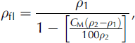
where ρ 1 is the fluid density, ρ 2 is the densifier density in kgm–3 and C M is the mass concentration of densifier in %. It is also commonly agreed that the pure ice-chip density is ρ ice = 920 kgm–3. We consider that, to a first approximation, the two-phase fluid compound (ice-chips/drilling-fluid) density ρ m can be calculated by the expression:
where α fl is the volume concentration of pure drilling fluid, α ice is the volume concentration of pure ice and ρ fl is the density of drilling fluid.
Viscosity Investigations
1. Viscosity of a two-component fluid compound
It is relatively easy to find relationships that give the viscosity of compound fluids. All the relationships found in the literature have been established for Newtonian fluids, with solid spherical particles in suspension. The relationship that can be used in most conditions, established by Reference Ishii and MishimaIshii and Mishima (1984), predicts the viscosity of a two-phase fluid for all types of spherical particles and even for high particle concentration:
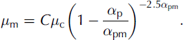
where μm is the two-phase fluid equivalent dynamic viscosity (cP), μc is the pure fluid dynamic viscosity in a two-phase fluid (cP), αp is the proportion of solid particles in a two-phase fluid and αpm (=0.62) is the maximum piling concentration (maximum spherical particle concentration) of solid particles.
2. Viscosity investigations of two-phase drilling compound using commercial viscosimeter
A commercial viscosimeter has been used for direct measurement of the dynamic viscosity of the binary drilling fluid and for the two-phase drilling compound. The viscosimeter is a TVe-05 (Fig. 1) from the Jean Lamy company.

Fig. 1 Commercial viscosimeter Lamy TVe-05. A d.c. motor drives an axle in rotation. The viscosity is deduced from the torque measured to keep the axle a constant speed. T is the torsion spring, D is the display for the viscosity value, R is the a.c. motor rotor, S is the a.c. motor stator, M is the moving body in the fluid and V the vessel in which the fluid is placed.
The viscosity of pure water and pure drilling fluid has been measured at different temperatures in order to verify the calibration of the viscosimeter. The measurement values have been compared with the theoretical values for water or with measurements already made by Reference Talalay and GundestrupTalalay and Gundestrup, 1999 for the binary drilling fluid. For the binary drilling fluid, the viscosimeter results have also been compared with the empirical relationship (from Reference Dubovkin, Malanicheva, Massur, Yu and FedorovDubovkin and others, 1985):

with
where T K (K) is the temperature, ν (cSt) is the kinematic viscosity and μ is the dynamic viscosity (cP). Coefficients C and D have been determined for the binary drilling fluid (D60 and HCFC-141b) (Reference Gundestrup, Clausen, Hansen and JohnsenGundestrup and others, 1994). In this case, C = 333.4 and D = 1.6.
The measurements obtained with the viscosimeter were very close to the results of Reference Talalay and GundestrupTalalay and Gundestrup, 1999, with <10% deviation (Fig. 2). Given this calibration, measurements on the real two-phase drilling-fluid compound (ice chips and drilling fluid: Exxsol D60 and HCFC-141b) were made using real ice chips (obtained after machining ice in a cold room with a drill head) or small polystyrene balls (0.7mm diameter; Fig. 3). These solid particles are about the same size as real ice chips, and nearly the same density as ice (920 kgm–3). The measurements were performed at different temperatures and for different volumetric solid particle concentration. The results (Fig. 4) fit well with the theory for spherical particles, but not for flat particles such as ice chips. It seems that viscosity of this two-phase fluid is linked to the particle geometry.
Fig. 2 Comparison of the viscosity at various temperatures for different fluids measured with an industrial (Lamy TVe-05) viscosimeter, with theoretical values (for water), and calculated according to the empirical relationship from Reference Talalay and GundestrupTalalay and Gundestrup, 1999.
Fig. 3 Photo of small polystyrene balls with diameter 0.7 mm.
Fig. 4 Viscosity of binary drilling fluid (D60 and HCFC-141b) with different types of solid particles in suspension.
3. Viscosity investigations of two-phase drilling compound using an experimental set-up
Viscosity measurements were made using an experimental set-up (Fig. 5) with water with temperature in the range 10– 15˚C instead of the binary drilling fluid in the range 0 to –20˚C. At this temperature, water viscosity is in the same range as the binary drilling-fluid dynamic viscosity, i.e. 1.2– 1.3 cP. Small polystyrene balls or thin plastic strips (Fig. 6) were used instead of real ice chips. This experimental method is more accurate than the commercial viscosimeter for high ice concentration (for high solid particle concentration). The choice of water at 10–15˚C was made to simplify the experimental procedure so that a greater number of tests could be performed. Although the density of the polystyrene strips does not ideally match the water density, we never observed settling of the strips, and conclude that the 10% density mismatch does not disturb our measurements. These experimental measurements (at constant temperature, with different ice concentration or particle shapes) were performed in order to establish a general link between viscosity and particle geometry, which could be extended to many situations, not just ice-drilling fluids.
Fig. 5 Photograph of the experimental set-up. Total dimensions are length 0.8 m, width 0.8 m, height 1.8 m. The fluid flow is maintained by a peristaltic pump powered by an a.c. motor. A pressure drop is measured between two points separated by 1m, with two mercury manometers. A peristaltic pump maintains a fluid flow rate with particles in suspension. The fluid is provided to the lower part of the cylinder through a pipe. At the bottom and at the top of the cylinder, where the pressure drop is measured, a mercury pressure gauge is plugged. The fluid returns to the pump through a filter, which retains the solid particles.
Fig. 6 Photo of small polystyrene thin strips: L = 1.5 mm, l = 0.3 mm, h = 0.1 mm.
The method is based on the Couette principle, which allows calculation of the apparent viscosity of a fluid mixture from the measured pressure drop in the flow within a gap between two coaxial cylinders considered infinitely long. The viscosity can be expressed (Reference MityarMityar, 2006) with parameters which can be measured with this set-up:
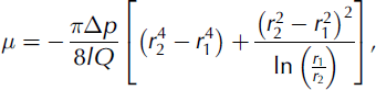
where Q is the flow rate (m3 s–1), l is the length (here 0.5 m) of the two tubes where the pressure drop, Δp, is measured, and r 1 (here 0.113 m) and r 2 (here 0.103 m) denote the diameter of the two cylinders.
Experiments have been carried out for different volumetric fractions of polystyrene balls and thin plastic strips, starting from 100% plastic balls (and no thin strips) up to 100% thin plastic strips (Fig. 7).
Fig. 7 Pressure drop measured between the entrance section and the exit section of the experimental set-up versus volumetric fraction of solid particles.
These results also show a high dependency of viscosity on particle geometry. It seems that there is a linear behaviour of
the viscosity with volumetric fraction of particles (Fig. 8). Thus, a correction factor has been introduced in order to find a relationship that takes into account both the particles’ geometry and concentration (Fig. 9):
Fig. 8 Viscosity deduced from the pressure-drop measurements versus volumetric fraction of solid particles for different types of solid particle.
Fig. 9 Correction factor (obtained by dividing the viscosity of a fluid with solid particles in suspension by the viscosity of the same fluid that should be obtained while using the Ishii empirical relationship) versus volumetric fraction of solid particles (spherical or thin strips).
where μ exp is the experimental viscosity (cP) and μ Ishii is the value of the viscosity obtained by calculation with the Ishii relationship (cP). The results suggest that the form of the correction factor C could be expressed as:
with different values for A and B (Table 1), which depend upon the volumetric fraction of balls and thin strips.
Table 1. Parameters for the calculation of the correction factor

This relationship has been used to calculate the viscosity of the two-phase fluid (D60/HCFC-141b and solid particles) for different concentrations of small particles or for ice chips (considered as thin strips). The results have been compared with the measurements made during this study both for spherical particles and for ice chips (Fig. 10). The uncertainty between the empirical relationship (taking into account the correction factor) and the experimental results is lower than 5%. Consequently, the mean viscosity of a drilling compound (drilling fluid and ice chips) can be expressed as:
Fig. 10 Comparison between measured viscosity of drilling fluid with ice chips in suspension and calculated viscosity using the Ishii relationship with the correction coefficient for drilling fluid with thin strips in suspension.
Conclusion
The goal of this study was the characterization, to first-order precision, of the main physical properties (i.e. viscosity and density) of a two-phase fluid at different temperatures and for various concentrations of solid particles. From our knowledge of these two parameters, it is possible to perform calculations and pursue numerical modelling of the behaviour of the two-phase flow around an ice-core drilling head (mainly with simple modelling software integrated with drawing software like Flow Works). It has been established that the mean drilling-fluid viscosity (together with ice chips) will increase with particle size or with particle concentration, and that this viscosity is highly linked with the solid particle geometry.


