2 $(X, Y)$ -invariant operators

Let $\mathcal {H}$ , $\mathcal {K}$ be Hilbert spaces. Let X be a bounded linear operator on $\mathcal {H}$ , i.e., $X\in \mathcal {B}(\mathcal {H})$ . Let $Y\in \mathcal {B}(\mathcal {K})$ , and let $H\subset \mathcal {H}$ , $K\subset \mathcal {K}$ be closed subspaces. We will use the notation

(2.1) $$ \begin{align} H_X=\{f\in H: Xf\in H\}\quad \text { and } \quad K_Y=\{g\in K : Yg\in K\}. \end{align} $$

An operator $A\in \mathcal {B}(H,K)$ is called $(X,Y)$ -invariant if and only if we have

(2.2) $$ \begin{align} \langle AXf,g\rangle=\langle Af,Yg \rangle \quad \text{for all }\quad f\in H_X, g\in K_Y. \end{align} $$

In particular, if $X\in \mathcal {B}(\mathcal {H})$ and $A\in \mathcal {B}(H)$ , we say that A is X-invariant if and only if

(2.3) $$ \begin{align} \langle AXf,g\rangle=\langle Af,X^*g \rangle \quad \mathrm{for}\quad f\in H_X, g\in H_{X^*}, \end{align} $$

i.e., A is $(X,X^*)$ -invariant.

Now let $P_{H_X}$ denote the orthogonal projection

$$ \begin{align*} P_{H_X}\colon \mathcal{H} \to H_X. \end{align*} $$

We will also denote by $P_{H_X}$ , whenever the context is clear, the orthogonal projection from H onto $H_X$ .

Note that if X is a co-isometry, i.e., $XX^*=I$ , then

(2.4) $$ \begin{align} f\in H_{X^*} \ \text{ if and only if }\ X^*f\in H_X. \end{align} $$

Proof Note that, for all $f\in H_X$ and $g_1\in K_{Y^*}$ , we have

$$ \begin{align*}\langle AXf,Y^*g_1\rangle=\langle YAXf,g_1 \rangle=\langle P_{K_{Y^*}}(YAXf), g_1\rangle\end{align*} $$

and

$$ \begin{align*}\langle Af,g_1 \rangle =\langle P_{K_{Y^*}}(Af), g_1\rangle.\end{align*} $$

Thus, the lemma holds.

Proof Let $f\in H_X$ and $g_1=YY^*g_1\in K_{Y^*}$ . Then, by (2.4), $g=Y^*g_1\in K_Y$ . Since A is $(X,Y)$ -invariant, then

$$ \begin{align*}\langle AXf,Y^*g_1 \rangle =\langle Af, YY^* g_1\rangle=\langle Af, g_1\rangle.\end{align*} $$

Now the result follows from Lemma 2.2.

Proof For all $f_1\in H_{X^*}$ , $g_1\in K_{Y^*}$ , we have that $X^*f_1\in H_X$ , $Y^*g_1\in K_Y$ , and

$$ \begin{align*}\langle AX^* f_1,g_1\rangle=\langle AX^*f_1, YY^*g_1\rangle=\langle AXX^*f_1,Y^*g_1\rangle=\langle Af_1,Y^*g_1\rangle.\\[-32pt]\end{align*} $$

Denote

$$\begin{align*}\mathcal{S}(X,Y)=\{A\in \mathcal{B}(H,K)\colon A \text{ is } (X,Y)\text{-invariant}\}.\end{align*}$$

Clearly, $\mathcal {S}(X,Y)$ is a subspace of $\mathcal {B}(H,K)$ .

Let $\varphi \in L^{\infty }$ . The linear operator $T_{\varphi }\in \mathcal {B}(H^2)$ is called a Toeplitz operator with the symbol $\varphi $ if

(2.5) $$ \begin{align}T_{\varphi} f=P_{H^2}(\varphi f)\qquad\text{ for}\quad f\in H^2. \end{align} $$

The Toeplitz operator $T_z$ is usually denoted by S and identified with the unilateral shift. Due to the Brown–Halmos characterization of Toeplitz operators, that is, $A\in \mathcal {B}(H^2)$ is a Toeplitz operator if and only if $S^*AS=A$ , we have the following.

Example 2.7 Let $\mathcal {H}=H=H^2=\mathcal {K}=K$ , $X=S=T_z$ , $Y=S^*$ . Then $H_X=K_{Y^*}=H^2$ and (3) in Proposition 2.5 is just Brown–Halmos condition, $S^*AS=A$ . Therefore, $A\in \mathcal {B}(H^2)$ is a Toeplitz operator if and only if it is S-invariant, ( $(S,S^*)$ -invariant).

Note also that taking $\mathcal {H}=\mathcal {K}=L^2$ , $X=M_z$ , $Y=M_{\bar z}$ and $H=K=H^2$ , $H_X=K_{Y^*}=H^2$ , then (3) in Proposition 2.5 gives

$$\begin{align*}A=P_{H^2}A_{|_{H^2}}=P_{H^2}M_{\bar z}A{M_z}_{|_{H^2}}=S^*AS.\end{align*}$$

So we also can say that $A\in \mathcal {B}(H^2)$ is a Toeplitz operator if and only if it is $M_z$ -invariant,( $(M_z,M_{\bar z})$ -invariant).

It is also worth noting that, by Proposition 2.5, each Toeplitz operator $A=T_{\varphi }$ , $\varphi \in L^{\infty }$ , is $(M_{\bar z},M_{z})$ -invariant. Indeed, for all $f\in (H^2)_{M_{\bar z}}$ , $g\in (H^2)_{M_z}$ , we have

(2.6) $$ \begin{align} \langle T_{\varphi} M_{\bar z}f, g \rangle=\langle \varphi \bar z f, g\rangle=\int_{\mathbb{T}}\varphi \bar z f\bar g dm=\langle \varphi f, zg\rangle =\langle T_{\varphi} f, M_z g\rangle. \end{align} $$

Recall the definition of Hankel operators. Let $J\in \mathcal {B}( L^2)$ , $(Jf)(z)=\bar z f(\bar z)$ . Denote by $\Gamma _{\psi }$ the Hankel operator with symbol $\psi \in L^{\infty }$ defined as $\Gamma _{\psi } \colon H^2\to H^2$ , $\Gamma _{\psi } f=P_{H^2}J\psi f$ for $f\in H^2$ . It is known that an operator $\Gamma \in \mathcal {B}(H^2)$ is a Hankel operator if and only if

(2.7) $$ \begin{align} S^*\Gamma=\Gamma S. \end{align} $$

Hence, we have the following.

Let $\alpha ,\theta $ be nonconstant inner functions. Consider the model spaces $K^2_{\alpha }=H^2\ominus \alpha H^2$ and $K^2_{\theta }=H^2\ominus \theta H^2$ , and let $P_{\alpha }$ , $P_{\theta }$ denote the orthogonal projections from $L^2$ onto $K^2_{\alpha }$ and $ K^2_{\theta }$ , respectively. It is known that $K^2_{\alpha } \cap L^{\infty }$ is dense in $K^2_{\alpha }$ . Let $\varphi \in L^2$ . Define

(2.8) $$ \begin{align}A^{\alpha,\theta}_{\varphi} f=P_{\theta}(\varphi f)\qquad\text{ for}\quad f\in K^2_{\alpha}\cap L^{\infty}.\end{align} $$

If $A^{\alpha ,\theta }_{\varphi }$ can be extended to a bounded operator from $K^2_{\alpha }$ to $K^2_{\theta }$ , i.e., $A^{\alpha ,\theta }_{\varphi }\in \mathcal {B}(K^2_{\alpha },K^2_{\theta })$ , then it is called the asymmetric truncated Toeplitz operator [Reference Câmara, Jurasik, Kliś-Garlicka and Ptak3]. In particular, if $\theta =\alpha $ , it is called a truncated Toeplitz operator and the notation $A^{\alpha }_{\varphi } =A^{\alpha ,\alpha }_{\varphi }$ will be used. In [Reference Sarason30], Sarason showed that an operator $A\in \mathcal {B} (K^2_{\theta })$ is a truncated Toeplitz operator if and only if

(2.9) $$ \begin{align}\langle Azf,zg\rangle=\langle Af,g \rangle\quad\text{for}\quad f,g\in K^2_{\theta} \,\text{ such that }\ zf,zg\in K^2_{\theta}\end{align} $$

and called this property shift-invariance. In [Reference Gu, Łanucha and Michalska17], this characterization was extended to the asymmetric case.

Example 2.10 Recall now the notion of (asymmetric) truncated Hankel operators [Reference Gu, Łanucha and Michalska17]. Let $\varphi \in L^2$ . Define

(2.10) $$ \begin{align}B^{\alpha,\theta}_{\varphi} f=P_{\theta} J(\varphi f)\qquad\text{ for}\quad f\in K^2_{\alpha}\cap L^{\infty}.\end{align} $$

and assume that $B^{\alpha ,\theta }_{\varphi }$ can be extended to a bounded operator from $K^2_{\alpha }$ to $K^2_{\theta }$ . We skip the word “asymmetric” if $\alpha =\theta $ . To give one more example of definition (2.2), let us take $\mathcal {H}=\mathcal {K}=L^2$ , $H={K^2_{\alpha }}$ , $K={K^2_{\theta }}$ and $X=M_z$ , $Y=M_{ z}$ . It can be easily shown using [Reference Gu, Łanucha and Michalska17, Proposition 4.2(b)] that an operator is an (asymmetric) truncated Hankel operator if and only if it is $(M_{ z}, M_z)$ -invariant.

We will be particularly interested in compressions of multiplication operators to several closed subspaces of $\mathcal {H}=L^2$ . If $H, K\subset L^2$ are closed and $\varphi \in L^{\infty }$ , let

$$ \begin{align*} T_{\varphi}^{H, K}=P_K M_{\varphi} P_H|_{H}. \end{align*} $$

If $K=H$ , we write $T_{\varphi }^{H}$ . These are particular cases of the so-called general Wiener–Hopf operators [Reference Böttcher and Speck1, Reference Devinatz and Shinbrot13, Reference Speck31], which we call general Toeplitz operators [Reference Câmara, O’Loughlin and Partington6].

Proof Let $f\in H_X, g\in K_{X^*}$ . Then

$$ \begin{align*}\langle T_{\varphi}^{H, K} Xf,g\rangle = \langle P_K \varphi Xf,g\rangle = \langle \varphi Xf,g\rangle.\end{align*} $$

On the other hand,

$$ \begin{align*}\langle X\varphi f,g\rangle =\langle \varphi f,X^*g\rangle= \langle P_K \varphi f,X^*g\rangle=\langle T_{\varphi}^{H, K} f,X^*g\rangle.\\[-35pt]\end{align*} $$

3 Invariance and preannihilator

In this section, we will consider $(X, Y)$ -invariance from a different point of view. For that we use the language of preannihilators and rank-one and rank-two operators in the preannihilator. Let $\mathcal {H}$ , $\mathcal {K}$ be separable Hilbert spaces. Each rank-one operator from $\mathcal {K}$ to $\mathcal {H}$ is usually denoted by $x\otimes y$ , where $x\in \mathcal {H}$ , $y\in \mathcal {K}$ , and it acts as $(x\otimes y)h=\langle h,y\rangle x$ for $h\in \mathcal {K}$ . The weak* topology (ultraweak topology) in $\mathcal {B}(\mathcal {H},\mathcal {K})$ is given by trace class operators of the form $t=\sum _{n=0}^{\infty } x_n\otimes y_n$ with $x_n\in \mathcal {H}$ , $y_n\in \mathcal {K}$ such that $\sum _{n=0}^{\infty } \|x_n\|^2< \infty $ , $\sum _{n=0}^{\infty } \|y_n\|^2< \infty $ . Let $\mathcal {B}_1(\mathcal {K},\mathcal {H})$ denote the space of all such trace class operators and $\|\cdot \|_1$ be the trace norm. Denote also by $\mathcal {F}_k$ the set of all operators in $\mathcal {B}_1(\mathcal {K},\mathcal {H})$ of rank at most k. Note that $\mathcal {B}(\mathcal {H},\mathcal {K})$ is a dual space to $\mathcal {B}_1(\mathcal {K},\mathcal {H})$ (see [Reference Meise and Vogt24, Chapter 16] for details) and the dual action is given by

$$\begin{align*}\mathcal{B}(\mathcal{H},\mathcal{K})\ \times \ \mathcal{B}_1(\mathcal{K},\mathcal{H})\ni(T,t)\ \mapsto\ <T,t>=\sum_{n=0}^{\infty} \langle Tx_n,y_n\rangle.\end{align*}$$

For a closed subspace $\mathcal {S}\subset \mathcal {B}(\mathcal {H},\mathcal {K})$ , the preannihilator of $\mathcal {S}$ is defined as

$$\begin{align*}\mathcal{S}_{\perp}=\{t\in B_1(\mathcal{K},\mathcal{H})\colon <T,t>=0 \text{ for all } T\in\mathcal{S} \}.\end{align*}$$

Let $\mathcal {N}\subset \mathcal {B}_1(\mathcal {K},\mathcal {H})$ . Recall that the annihilator of $\mathcal {N}$ is given by

$$ \begin{align*}\mathcal{N}^{\bot}=\{T\in \mathcal{B}(\mathcal{H},\mathcal{K})\colon <T,t>=0 \text{ for all } t\in \mathcal{N} \}.\end{align*} $$

We will usually write, for $T\in \mathcal {B}(\mathcal {H}, \mathcal {K})$ and $t\in \mathcal {B}_1(\mathcal {K},\mathcal {H})$ , that $T\perp t$ if and only if $<T,t>=0$ . Note that $\mathcal {S}\subset \mathcal {B}(\mathcal {H},\mathcal {K})$ is weak*-closed if and only if $\mathcal {S} = (\mathcal {S}_{\perp })^{\perp }$ . Recall after [Reference Larson21] that a weak ${}^*$ -closed subspace $\mathcal {S}\subset \mathcal {B}(\mathcal {H},\mathcal {K}) $ is called k-reflexive ( $k=1, 2,3,4\dots $ ), if $\mathcal {S}=\big (\mathcal {S}_{\bot }\cap \mathcal {F}_k\big )^{\perp }$ .

Now we recall previous definitions (Definitions 1.2–1.4) from this perspective.

Now we present a result concerning the topological behavior of the subspace of all $(X,Y)$ -invariant operators.

Proposition 3.2 Let $H\subset \mathcal {H}$ and $K\subset \mathcal {K}$ . Let $A\in \mathcal {B}(H,K)$ and $X\in \mathcal {B}(\mathcal {H})$ , $Y\in \mathcal {B}(\mathcal {K})$ . Then

$$\begin{align*}\mathcal{S}(X,Y)=\{A\in \mathcal{B}(H,K)\colon A \text{ is } (X,Y)\text{-invariant}\}\end{align*}$$

is $2$ -reflexive.

Proof Note that for $A\in \mathcal {B}(H,K)$ condition (2.2) is equivalent to

(3.5) $$ \begin{align} <A, Xf\otimes g-f\otimes Yg>=0\qquad \text{for}\qquad f\in H_X, g\in K_Y. \end{align} $$

Let us denote

(3.6) $$ \begin{align} \mathcal{N}=\Big\{Xf\otimes g-f\otimes Yg\colon\ f\in H_X, g\in K_Y \Big\}. \end{align} $$

By (3.5), we have

(3.7) $$ \begin{align} \mathcal{S}(X,Y)_{\perp}\supset \mathcal{N}\quad\quad\text{and }\quad\quad{\mathcal{S}(X,Y)}\supset \mathcal{N}^{\perp}. \end{align} $$

Thus

$$ \begin{align*}(\mathcal{S}(X,Y)_{\perp})^{\perp}\subset \mathcal{N}^{\perp}\subset \mathcal{S}(X,Y).\end{align*} $$

Hence, $\mathcal {S}(X,Y)$ is weak*-closed (WOT-closed), since it is characterized by annihilating some trace class (finite rank) operators. Moreover, $\mathcal {S}(X,Y)$ is $2$ -reflexive because

$$ \begin{align*} \Big(\mathcal{S}(X,Y)_{\perp} \cap \mathcal{F}_2\Big)^{\perp}\subset\Big(\mathcal{N}\cap\mathcal{F}_2\Big)^{\perp}=\mathcal{N}^{\perp}\subset\mathcal{S}(X,Y).\\[-37pt] \end{align*} $$

4 Kernels of $(X, Y)$ -invariant operators

It is a well-known property that kernels of Toeplitz operators are nearly $S^*$ -invariant. It was also proved in a recent paper [Reference O’Loughlin27] that kernels of truncated Toeplitz operators are nearly $S^*$ -invariant with defect not greater than $1$ . More generally, in this section, we study the invariance properties of the kernels of $(X,Y)$ -invariant operators.

One may look at the property of near X-invariance of a space $\mathcal {L}\subset H$ as meaning that, for any element $f\in \mathcal {L}$ , either $Xf$ is also in $\mathcal {L}$ , or it does not belong to H. In other words, looking at how X acts on elements of $\mathcal {L}$ , we see that either $(i) \; Xf\in \mathcal {L}$ , or $(ii)\, Xf\in H\setminus \mathcal {L}$ , or $(iii)\, Xf\in \mathcal {H}\setminus H$ ; if $\mathcal {L}$ is nearly X-invariant, then only $(i)$ and $(iii)$ can hold.

It is thus natural to ask, when $\mathcal {L}=\ker A$ , where $A\in \mathcal {B}(H, K)$ , for which elements $f\in \ker A$ does each of the properties $(i)$ – $(iii)$ hold.

On may also consider the question of describing the part $\mathcal {L}$ of $\ker A$ such that $X^*\mathcal {L}\subset \ker A$ , or $X^*\mathcal {L}\subset H$ , and compare with the analog results for X. Indeed, these questions are related, since we have, for co-isometric X,

(4.1) $$ \begin{align} (\ker A)_{X^*}\subset X(\ker A)_X. \end{align} $$

To see this note that, by (2.4), $f\in (\ker A)_{X^*}$ if and only if $X^*f\in (\ker A)_X$ . It follows that $f=XX^*f\in X(\ker A)_X$ . Note also that if X is unitary, then

$$ \begin{align*}(\ker A)_{X^*}= X(\ker A)_X.\end{align*} $$

Our first result is a very simple but fundamental one, when considering those questions. Let $ (\mathcal {L})_{H}^{\bot }=H\ominus \mathcal {L}$ for any closed subset $\mathcal {L}\subset H$ .

We have the following.

Proposition 4.1 Let $H\subset \mathcal {H}$ and $K\subset \mathcal {K}$ . Let $A\in \mathcal {B}(H,K)$ and $X\in \mathcal {B}(\mathcal {H})$ , $Y\in \mathcal {B}(\mathcal {K})$ . If A is $(X,Y)$ -invariant, then

$$ \begin{align*} AXf\in (K_{Y})_K^{\bot} \quad \text{for all}\quad f\in \ker A\cap H_X. \end{align*} $$

Proof If $f\in \ker A$ and $Xf\in H$ , then, for all $g\in K_Y$ ,

$$ \begin{align*} \langle AXf,g\rangle = \langle Af,Yg\rangle=0, \quad \text{since}\quad Af=0.\\[-32pt] \end{align*} $$

As a consequence, we obtain the following necessary and sufficient condition for $\ker A$ to be nearly X-invariant.

Proof If $AXf\in K_Y$ for all $f \in \ker A\cap H_X$ , then by Proposition 4.1, we have $AXf=0$ for all $ f\in \ker A\cap H_{X}$ and $\ker A$ is nearly X-invariant w.r.t. H. Suppose now that there is $\tilde f\in \ker A\cap H_X$ with $AX\tilde f\notin K_Y$ (therefore, we necessarily have $AX\tilde {f}\neq 0$ , i.e., $X\tilde {f}\notin \ker A$ ). Define

$$ \begin{align*} \mathcal{I}=\{g\in (K_Y)_K^{\bot} : g=AXf \;\;\text{for same} \;\; f\in \ker A\cap H_X\}. \end{align*} $$

We have $\mathcal {I}\neq \{0\}$ because $AX\tilde f\neq 0$ and $AX\tilde f\in (K_Y)_K^{\bot }$ by Proposition 4.1. So let $\{g_1,g_2,\dots ,g_m\}$ , with $m\leqslant N$ , be a basis for $\mathcal {I}$ . For each $g_j$ , $j=1,2,\dots ,m$ , let $f_j$ be an element of $\ker A \cap H_X$ such that $g_j=AXf_j$ . We have that

$$ \begin{align*} A^{-1}\{g_j\}:=\{f\in H : Af=g_j\}=\{Xf_j+h\colon h\in \ker A\}. \end{align*} $$

Now take $h_j=(I-P_{\ker A})Xf_j\in A^{-1}\{g_j\}$ , which is such that $Ah_j=g_j$ and $h_j\in H \ominus \ker A$ . Then, for any $f\in \ker A\cap H_X$ , we have

$$ \begin{align*} AXf=\sum_{j=1}^mc_jg_j=\sum_{j=1}^m(c_jAh_j)=A\left(\sum_{j=1}^mc_jh_j\right), \end{align*} $$

with $c_j\in \mathbb {C}$ . Hence,

$$ \begin{align*} Xf-\sum_{j=1}^m c_jh_j \in \ker A \end{align*} $$

and we can write that

$$ \begin{align*} Xf\in \ker A\oplus \operatorname{\mathrm{span}}\{h_j\colon j=1,2,\dots,m\}.\\[-34pt] \end{align*} $$

Remark 4.5 From now on, we will use the notation

$$ \begin{align*} [h_j]_{j=1,\dots,m}:=\operatorname{\mathrm{span}}\{h_j \colon j=1,\dots,m\}. \end{align*} $$

We also define

$$ \begin{align*} H_X^A=\ker A\cap H_X. \end{align*} $$

Two simple examples illustrate these results.

5 Orthogonal decompositions of kernels

The study of near invariance properties for kernels of operators raises some natural questions. For instance, if $\ker A$ is nearly X-invariant w.r.t. H, which elements are kept in $\ker A$ under the action of X? If $\ker A$ is nearly X-invariant w.r.t. H with defect, which elements “stay” in H upon the action of X?

In this section, we show that the relations between $(X,Y)$ -invariance of an operator A and the near invariance properties of its kernel, with respect to X and Y, yield decompositions of the kernel in terms of orthogonal sums where the terms behave differently under the action of X. These decompositions generalize well-known decompositions of model spaces, such as those presented in the introduction.

To motivate the results that follow, we present two simple examples.

Example 5.1 (Model spaces)

Let $\theta $ be an inner function and assume, to begin with, that $\theta (0)=0$ . In this case, we have two decompositions

(5.1) $$ \begin{align} {K^2_{\theta}}=zK^2_{\frac{\theta}{z}}\oplus \mathbb{C}, \quad {K^2_{\theta}}=K^2_{\frac{\theta}{z}}\oplus \tfrac{\theta}{z}\mathbb{C}, \end{align} $$

where $\mathbb {C}=K^2_z$ . If $\theta (0)\neq 0$ , ${K^2_{\theta }}$ cannot be decomposed similarly in terms of $K^2_z$ and $K^2_{\frac {\theta }{z}}$ , but taking into account that ${K^2_{\theta }}=\ker T_{\bar \theta }$ and $K^2_{\frac {\theta }{z}}=\ker T_{\bar \theta z}$ , we can generalize (5.1) by writing

(5.2) $$ \begin{align} {K^2_{\theta}}&=z\ker T_{z\bar\theta}\oplus [k_0^{\theta}]=({K^2_{\theta}})_{\bar z}\oplus [k_0^{\theta}],\\ {K^2_{\theta}}&=\ker T_{z\bar\theta}\oplus [\tilde k_0^{\theta}]=({K^2_{\theta}})_z\oplus [\tilde k_0^{\theta}]\notag \end{align} $$

with

(5.3) $$ \begin{align} k_0^{\theta}=1-\overline{\theta(0)}\theta, \quad \tilde k_0^{\theta}=\bar z (\theta-\theta(0)). \end{align} $$

From the first decomposition in (5.2), we see that $\bar zK^2_{\theta }\subset K^2_{\theta } \oplus [\bar z]$ and

$$ \begin{align*} M_{\bar z}(z\ker T_{z\bar\theta})\subset {K^2_{\theta}}, \quad M_{\bar z}(k_0^{\theta})\in L^2\setminus H^2, \end{align*} $$

which reflects the fact that ${K^2_{\theta }}$ is nearly $M_{\bar z}$ -invariant w.r.t. $H^2$ .

From the second decomposition in (5.2), we see that $ zK^2_{\theta }\subset K^2_{\theta } \oplus [\theta ]$ (cf. [Reference Chalendar, Gallardo-Gutiérrez and Partington11], Proposition 2.2) and

$$ \begin{align*} M_z(\ker T_{z\bar\theta})\subset {K^2_{\theta}}, \quad M_z(\tilde k_0^{\theta})\in H^2\setminus {K^2_{\theta}}, \end{align*} $$

so we may interpret it as saying that ${K^2_{\theta }}$ is $H^2$ -invariant for $M_z$ and nearly S-invariant with defect $1$ , w.r.t. $H^2$ , therefore almost-invariant for S with defect $1$ .

These are well-known properties; still, they provide an interpretation of the equalities in (5.2) which will lead to future results generalizing model space decompositions.

Example 5.2 (Kernels of truncated Toeplitz operators on ${K^2_{\theta }}$ with analytic symbols)

The kernels of operators in this class are of the form $\gamma {K^2_{\beta }}$ , where $\gamma $ and $\beta $ are inner functions such that $\beta \leqslant \theta $ , $\gamma =\theta /\beta $ and $\beta $ divides $\psi _+^i$ -the inner factor of $\psi _+$ , [Reference Nikolski26], [Reference Câmara and Partington10, Theorem 7.2]. Let A be a truncated Toeplitz operator with $\ker A=\gamma {K^2_{\beta }}$ . Then, from (5.2), we have

(5.4) $$ \begin{align} \ker A=\gamma({K^2_{\beta}})_{\bar z}\oplus[\gamma k_0^{\beta}] \quad \text{with} \quad (\ker A)_{\bar z}=\gamma ({K^2_{\beta}})_{\bar z}. \end{align} $$

Let us assume that $\gamma (0)=0$ , in which case $\gamma {K^2_{\beta }}$ is not nearly $S^*$ -invariant. Note that, since $\gamma (0)=0$ , both terms of the orthogonal sum are mapped into $H^2$ by multiplication by $\bar z$ . On the other hand, only the elements of $(\ker A)_{\bar z}$ are mapped into $\ker A$ . We thus conclude that $\ker A$ is almost $S^*$ -invariant (or, equivalently, almost $S_{\theta }$ -invariant, where $S_{\theta }=A^{\theta }_z$ is the truncated shift) with defect $1$ and defect space $[\bar z\gamma k_0^{\beta }]$ .

These decompositions of the kernels of certain operators, in terms of direct sums of subspaces behaving in different ways under multiplication by z and $\bar z$ , can be seen as resulting from the relation between the shift-invariance of the operator and the invariance properties of their kernels, as we show next.

Recall that for $A\in \mathcal {B}(H,K)$ and $X\in \mathcal {B}(\mathcal {H})$ , $H\subset \mathcal {H}$ ,

(5.5) $$ \begin{align} H_{ X}^A=\ker A\cap H_X. \end{align} $$

Proposition 5.3 Let $A\in \mathcal {B}(H,K)$ and $X\in \mathcal {B}(\mathcal {H})$ , $H\subset \mathcal {H}$ . Then

$$ \begin{align*}\ker A=H_{ X}^A\oplus P_{\ker A}\, H_X^{\bot}.\end{align*} $$

Proof We have to prove that $H_{ X}^A$ is the orthogonal complement of $P_{\ker A}\,H_X^{\bot }$ in $\ker A$ . Let $f\in \ker A$ , $f \bot P_{\ker A}H_X^{\bot }$ . Then $f\bot H_X^{\bot }$ and so $f\in \ker A\cap H_X=H_{ X}^A$ .

Conversely, if $f\in H_{ X}^A$ , then, for all $g\in H_X^{\bot }$ ,

$$ \begin{align*} \langle f,P_{\ker A}\,g \rangle = \langle f, g\rangle=0 \end{align*} $$

because $f\in H_X$ and $g\in H_X^{\bot }$ .

Recall that

$$ \begin{align*} (\ker A)_X=\{f\in \ker A : Xf\in \ker A\}\subset H_{ X}^A. \end{align*} $$

In its turn, we can decompose $H_{ X}^A$ as follows.

Proposition 5.4 Let $X\in \mathcal {B}(\mathcal {H})$ , $Y\in \mathcal {B}(\mathcal {K})$ , $H\subset \mathcal {H}$ , $K\subset \mathcal {K}$ . If $A\in \mathcal {B}(H,K)$ is $(X,Y)$ -invariant, then

$$ \begin{align*} H_{ X}^A=(\ker A)_X\oplus P_{H^A_X}(X^*A^* K_Y^{\bot}), \end{align*} $$

where we abbreviate $(K_Y)^{\bot }_K$ to $K_Y^{\bot }$ .

Proof Let $f\in (\ker A)_X$ . Then obviously $AXf=0$ , and hence, for all $g\in K_Y^{\bot }$ , we have

$$ \begin{align*} 0=\langle AXf,g\rangle = \langle Xf,A^*g\rangle =\langle f, X^*A^*g\rangle= \langle f,P_{H_{ X}^A} (X^*A^*g)\rangle. \end{align*} $$

Therefore, $f\bot P_{H_{ X}^A}(X^*A^* K_Y^{\bot })$ for all $f\in (\ker A)_X$ . Conversely, let $f\in H_X^A$ and

(5.6) $$ \begin{align} f\bot P_{H_{ X}^A}(X^*A^* K_Y^{\bot}). \end{align} $$

For all $g\in K_{Y}$ , we have, by (2.2), $0=\langle AXf,g\rangle =\langle Af, Yg\rangle $ so

$$ \begin{align*} 0=\langle Xf,A^*g\rangle =\langle f, X^*A^*g\rangle =\langle f,P_{H^A_X} (X^*A^*g)\rangle. \end{align*} $$

Hence,

(5.7) $$ \begin{align} f\bot P_{H^A_X} (X^*A^* K_{Y}). \end{align} $$

From (5.6) and (5.7), we conclude that, for $f\in (\ker A)_X$ , $f\bot P_{H^A_X}( X^*A^*K)$ , so for all $g\in K$ , we have

$$ \begin{align*} 0=\langle f,P_{H^A_X} (X^*A^*g)\rangle = \langle f, X^*A^*g\rangle = \langle AXf,g\rangle, \end{align*} $$

and hence $AXf=0$ , so $Xf\in \ker A$ and thus $f\in (\ker A)_X$ .

Clearly, $\ker A$ is nearly X-invariant w.r.t. H if and only if $H_{ X}^A=(\ker A)_X$ , so we have the following.

Corollary 5.5 Let $X\in \mathcal {B}(\mathcal {H})$ , $Y\in \mathcal {B}(\mathcal {K})$ , $H\subset \mathcal {H}$ , $K\subset \mathcal {K}$ . Assume that $A\in \mathcal {B}(H,K)$ is $(X,Y)$ -invariant. Then the subspace $\ker A$ is nearly X-invariant w.r.t. H if and only if $P_{H_{ X}^A}(X^*A^* K_Y^{\bot })=\{0\}$ , i.e., $\langle AXf,g\rangle =0$ for all $f\in H^A_X$ , $g\in K_Y^{\bot }$ .

The subspace $\ker A$ is nearly X-invariant w.r.t. H with defect if and only if

(5.8) $$ \begin{align} \dim P_{H_{ X}^A}(X^*A^*K_{Y}^{\bot})<\infty. \end{align} $$

As a consequence of the previous results, we have the following.

Theorem 5.6 Let $X\in \mathcal {B}(\mathcal {H})$ , $Y\in \mathcal {B}(\mathcal {K})$ , $H\subset \mathcal {H}$ , $K\subset \mathcal {K}$ . If $A\in \mathcal {B}(H,K)$ is $(X,Y)$ -invariant, then we have the orthogonal decomposition

(5.9) $$ \begin{align}\ker A=(\ker A)_X \oplus P_{H_{ X}^A}( X^* A^* K_Y^{\bot})\oplus P_{\ker A}H_X^{\bot}. \end{align} $$

Moreover, if X, Y are co-isometries, then A is $(X^*,Y^*)$ -invariant, and we have

(5.10) $$ \begin{align}\ker A=(\ker A)_{X^*} \oplus P_{H^A_{X^*}}( X A^* K_{Y^*}^{\bot})\oplus P_{\ker A}H_{X^*}^{\bot}. \end{align} $$

Corollary 5.7 Let $X\in \mathcal {B}(\mathcal {H})$ , $H\subset \mathcal {H}$ . If $A\in \mathcal {B}(H)$ is X-invariant, then we have the orthogonal decomposition

(5.11) $$ \begin{align}\ker A=(\ker A)_X \oplus P_{H_{ X}^A}( X^* A^* H_{X^*}^{\bot})\oplus P_{\ker A}H_X^{\bot}. \end{align} $$

Moreover, if X is a co-isometry, then A is $X^*$ -invariant, and we have

(5.12) $$ \begin{align}\ker A=(\ker A)_{X^*} \oplus P_{H^A_{X^*}}( X A^* H_{X}^{\bot})\oplus P_{\ker A}H_{X^*}^{\bot}. \end{align} $$

Remark 5.8 In (5.9), we have that $(\ker A)_X$ consists of the elements of $\ker A$ which are mapped into $\ker A$ by X;

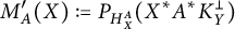(5.13) $$ \begin{align} M_A^{\prime}(X):=P_{H_{ X}^A}(X^*A^* K_Y^{\bot}) \end{align} $$

consists of elements which are mapped into $H \setminus \ker A$ by X; and

(5.14) $$ \begin{align} M_A^{\prime\prime}(X):=P_{\ker A}H_{X}^{\bot} \end{align} $$

consists of elements which are mapped into $\mathcal {H}\setminus H$ by X.

Similarly, having (5.10), we can consider the following spaces:

(5.15) $$ \begin{align}(\ker A)_{X^*};\quad M_A^{\prime}(X^*):=P_{H_{ X}^A}(XA^* K_{Y^*}^{\bot});\quad M_A^{\prime\prime}(X^*):=P_{\ker A}H_{X^*}^{\bot}. \end{align} $$

According to definitions (5.13) and (5.14), we have the following.

Corollary 5.10 Let $X\in \mathcal {B}(\mathcal {H})$ , $Y\in \mathcal {B}(\mathcal {K})$ , $H\subset \mathcal {H}$ , $K\subset \mathcal {K}$ . Assume that $A\in \mathcal {B}(H,K)$ is $(X,Y)$ -invariant. If $K_Y^{\bot }=\big [f_Y\big ]$ , $H_X^{\bot }=\big [f_{X}\big ]$ , then

$$ \begin{align*} \ker A=(\ker A)_X \oplus \big [P_{H_{ X}^A}( X^* A^*f_{ Y})\big]\oplus\big[ P_{\ker A}f_X\big]. \end{align*} $$

In this case, $\ker A$ is nearly X-invariant with defect at most $1$ .

Remark 5.11 With the same assumptions as in Corollary 5.10 and taking Corollary 5.9(1) into account, we have, for $f\in H_{ X}^A$ ,

$$ \begin{align*} Xf\in X(\ker A)_X \oplus [XP_{H_{ X}^A}(X^*A^*f_{Y})], \end{align*} $$

where the direct sum is orthogonal if X is unitary, and the second term in the sum gives the defect space for the near X-invariance of $\ker A$ .

We finish this section by establishing a relation between X-invariance and conjugations that will be used later. Recall that by a conjugation on $\mathcal {H}$ , we mean an antilinear operator which is involutive and isometric [Reference Garcia and Putinar16].

6 Toeplitz operators

Now we apply the previous results to kernels of Toeplitz operators. In what follows, we assume that $G \in L^{\infty }$ and $T_G\colon H^2\to H^2$ is defined by $T_Gf=P^+Gf$ for all $f\in H^2$ , where $P^+$ is the orthogonal projection from $L^2$ onto $H^2$ . Since, for any nonzero Toeplitz kernel strictly contained in $H^2$ , one can associate a unimodular symbol [Reference Câmara and Partington8, Reference Sarason29], we may assume that $|G|=1$ . We assume also that $\ker T_G\neq \{0\}$ . We have the following [Reference Câmara and Partington8, Reference Makarov and Poltoratski23].

Since the existence of a factorization such as described in Proposition 6.1 is in general difficult to verify, unless G belongs to some special class such as that of nonvanishing piecewise continuous functions on the unit circle $\mathbb {T}$ [Reference Mikhlin and Prössdorf25], one may alternatively consider the Riemann–Hilbert problem

(6.1) $$ \begin{align} Gf_+=f_- \quad \text{with}\quad f_+\in H^2, \; f_-\in H^2_-:=\bar z \overline{H^2}. \end{align} $$

Indeed, $\ker T_G$ consist of all solutions $f_+$ to this problem, so $\ker T_G\neq \{0\}$ if and only if there exists a nonzero solution to (6.1) (which may be obtained using a variety of methods developed to solve Riemann–Hilbert problems).

Consider $\mathcal {H}=\mathcal {K}=L^2$ and let $X=M_{\beta }$ , or simply $X=\beta $ , with $\beta $ inner, and $Y=X^*$ . We have that $T_G$ is $\beta $ -invariant by Corollary 2.12 and, in this case,

(6.2) $$ \begin{align} H=H^2, \; H_X=(H^2)_{\beta}=H^2, \; H_{X^*}=(H^2)_{\bar\beta}=\beta H^2, \end{align} $$

(6.3) $$ \begin{align} H_X^{\bot}=\{0\}, \; H_{X^*}^{\bot}={K^2_{\beta}}. \end{align} $$

To apply the decomposition given in Theorem 5.6, we first describe the spaces $(\ker T_G)_{\beta }$ and $(\ker T_G)_{\bar \beta }$ .

Proposition 6.2 Let $\beta $ be an inner function, and let $G\in L^{\infty }$ . Then

$$ \begin{align*} (\ker T_G)_{\beta} = \ker T_{\beta G};\qquad\qquad (\ker T_G)_{\bar\beta}= \beta \ker T_{\beta G}. \end{align*} $$

The decomposition theorem now yields the following.

Theorem 6.4 Let $G\in L^{\infty }$ and $\beta $ be an inner function. The following orthogonal decompositions hold:

(6.4) $$ \begin{align} \ker T_G =\ker T_{\beta G}\oplus P_{\ker T_G}(\bar G\bar z\overline{{K^2_{\beta}}})=(H^2)_{\beta}^{ T_G}; \end{align} $$

(6.5) $$ \begin{align} \ker T_G =\beta \ker T_{\beta G}\oplus P_{\ker T_G}{K^2_{\beta}}. \end{align} $$

Proof The decompositions follow from Corollary 5.7, Propositions 5.4 and 6.2, and (6.2) and (6.3). For (6.4), we took into account that, for $A=T_G$ ,

$$\begin{align*}P_{{H_{\beta}^A}}(\bar\beta P^+\bar G {K^2_{\beta}})=P_{\ker A}(\bar\beta P^+\bar G {K^2_{\beta}})= P_{\ker T_G}(\bar\beta \bar G{K^2_{\beta}})\end{align*}$$

and $\bar \beta \bar G {K^2_{\beta }}= \bar G\bar z \overline {{K^2_{\beta }}}$ .

Example 6.6 If $G=\bar \alpha $ , where $\alpha $ is an inner function, then $\ker T_G={K^2_{\alpha }}$ . If $\beta < \alpha $ , the decompositions (6.4) and (6.5) become

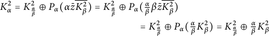$$ \begin{align*} {K^2_{\alpha}}=K^2_{\frac{\alpha}{\beta}}\oplus P_{\alpha}(\alpha\bar z \overline{{K^2_{\beta}}})=K^2_{\frac{\alpha}{\beta}} &\oplus P_{\alpha}(\tfrac{\alpha}{\beta} \beta \bar z \overline{{K^2_{\beta}}})\\ &\qquad =K^2_{\frac{\alpha}{\beta}}\oplus P_{\alpha}(\tfrac{\alpha}{\beta} {K^2_{\beta}})=K^2_{\frac{\alpha}{\beta}}\oplus \tfrac{\alpha}{\beta} {K^2_{\beta}} \end{align*} $$

and

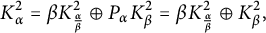$$ \begin{align*} {K^2_{\alpha}}=\beta K^2_{\frac{\alpha}{\beta}}\oplus P_{\alpha} {K^2_{\beta}}=\beta K^2_{\frac{\alpha}{\beta}}\oplus {K^2_{\beta}}, \end{align*} $$

and we recover the known decompositions for ${K^2_{\alpha }}$ ,

(6.6) $$ \begin{align} {K^2_{\alpha}}=K^2_{\frac{\alpha}{\beta}}\oplus \tfrac{\alpha}{\beta} {K^2_{\beta}}, \qquad {K^2_{\alpha}}=\beta K^2_{\frac{\alpha}{\beta}}\oplus {K^2_{\beta}}. \end{align} $$

Now consider, for a given inner function $\alpha $ , the usual conjugation $C_{\alpha }$ in $L^2$ given by $C_{\alpha } f=\alpha \bar z \bar f$ . This conjugation leaves the model space ${K^2_{\alpha }}$ invariant, i.e., $C_{\alpha } {K^2_{\alpha }}={K^2_{\alpha }}$ . Moreover, as shown in [Reference Câmara, Kliś-Garlicka, Łanucha and Ptak4], it is the only (up to multiplication by a constant of modulus 1) conjugation C such that $CM_z=M_{\bar z}C$ and $C{K^2_{\alpha }}\subset {K^2_{\alpha }}$ . It is not difficult to see that this unique conjugation $C_{\alpha }$ maps the two decompositions (6.6) onto each other, i.e.,

(6.7) $$ \begin{align} C_{\alpha}(K^2_{\frac{\alpha}{\beta}})=\beta K^2_{\frac{\alpha}{\beta}}, \qquad C_{\alpha}(\tfrac{\alpha}{\beta} {K^2_{\beta}})={K^2_{\beta}}. \end{align} $$

Recently, in [Reference Dymek, Płaneta and Ptak14], it was shown that, for a given unimodular function G, the only (up to multiplication by a constant of modulus 1) conjugation C such that $CM_z=M_{\bar z}C$ and $C\ker T_G\subset \ker T_G$ has the form

(6.8) $$ \begin{align} C_Gf=\bar G\bar z\bar f, \; f\in L^2. \end{align} $$

Using this conjugation, the results in (6.7) may be generalized for all Toeplitz kernels as follows.

Proposition 6.7 Let $G\in L^{\infty }$ be a unimodular function, and let $C_G$ be the conjugation defined by (6.8). Then

(6.9) $$ \begin{align} {C}_G(\ker T_G)_{\bar\beta}=(\ker T_G)_{\beta}, \end{align} $$

(6.10) $$ \begin{align} {C}_G(P_{\ker T_G}{K^2_{\beta}})=P_{\ker T_G}({C}_G {K^2_{\beta}})=P_{\ker T_G}(\bar G\bar z \overline{{K^2_{\beta}}}). \end{align} $$

We thus have, as it happened in the case of model spaces:

The following example also raises an interesting question.

Example 6.9 Let $|G|=1$ and take $\beta =z$ . If $G=\bar \theta $ , then $\ker T_G={K^2_{\theta }}$ . Since $P_{\theta } (\bar z\theta )=\tilde k_0^{\theta }$ , we have

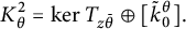(6.11) $$ \begin{align} {K^2_{\theta}}=\ker T_{z\bar\theta}\oplus [\tilde k_0^{\theta}]. \end{align} $$

In Example 6.9, $\tilde k_0^{\theta }$ is a maximal function for the Toeplitz kernel ${K^2_{\theta }}$ , i.e., it cannot belong to any Toeplitz kernel strictly contained in ${K^2_{\theta }}$ , such as $\ker T_{z\bar \theta }$ [Reference Câmara and Partington7]. However, (6.11) tells us furthermore that there exists a maximal function for ${K^2_{\theta }}$ which is orthogonal to $\ker T_{z\bar \theta }=({K^2_{\theta }})_z$ .

This raises the following question: given any Toeplitz kernel, $\ker T_G$ , is there a maximal function which is orthogonal to $(\ker T_G)_z$ ? Since, from (6.4),

$$ \begin{align*} \ker T_G=(\ker T_G)_z \oplus [P_{\ker T_G}(\bar z\bar G)], \end{align*} $$

that question in equivalent to asking whether $P_{\ker T_G}(\bar z\bar G)$ is a maximal function for $\ker T_G$ .

It was shown in [Reference Câmara and Partington7] that every Toeplitz kernel has a maximal function and, in [Reference Câmara, Malheiro and Partington5, Reference Câmara and Partington8] that $f_M$ is a maximal function for $\ker T_G$ if and only if $Gf_M=\bar z\bar h$ , where $h\in H^2$ is outer. We have

$$ \begin{align*} P_{\ker T_G}(\bar z\bar G)=P_{\ker T_G}({C}_G1)={C}_G(P_{\ker T_G}1)=\bar z\bar G \overline{P_{\ker T_G}1} \end{align*} $$

and thus

$$ \begin{align*} GP_{\ker T_G}(\bar z\bar G)=\bar z \overline{P_{\ker T_G}1}. \end{align*} $$

Therefore, $P_{\ker T_G}(\bar z\bar G)$ is a maximal function for $\ker T_G$ if and only if $P_{\ker T_G}1$ is outer. Now, using Hitt’s/Hayashi’s representation $\ker T_G=g K_I$ (Theorem 1.1), where g is an outer function, and the expression for $P_{\ker T_G}$ given in [Reference Hartmann and Ross18], we have

$$ \begin{align*} P_{\ker T_G}1=gP_I\bar g\cdot 1 =gIP^-\bar IP^+\bar g=g \,\overline{g(0)}(1-\overline{I(0)}I) \end{align*} $$

which is outer, since $g(0)\neq 0$ . We have thus proved the following.

Proposition 6.10 Let $G\in L^{\infty }$ be a unimodular function. There exists a maximal function $f_M$ in $\ker T_G$ such that

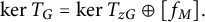$$ \begin{align*} \ker T_G=\ker T_{zG}\oplus [f_M]. \end{align*} $$

If $\ker T_G=g K_I$ is Hitt’s representation of $\ker T_G$ according to Theorem 1.1, then such a maximal function is given by

$$ \begin{align*} f_M=P_{\ker T_G}(\bar z\bar G) =\bar z\bar G \bar g\,g(0)(1-I(0)\bar I). \end{align*} $$

7 Truncated Toeplitz operators

Now we apply the previous results to truncated Toeplitz operators, for $X=\bar \beta $ and $X=\beta $ , identifying as before $M_{\alpha }$ with $\alpha $ , for $\alpha \in L^{\infty }$ .

Let $\theta ,\beta $ be nonconstant inner functions. Consider the model space $K^2_{\theta }\subset L^2$ and the operator $X=M_{\bar \beta }$ (we will simply write $X=\bar \beta $ ). Let $G\in L^{\infty }$ , and let $A_G^{\theta } \colon {K^2_{\theta }} \to {K^2_{\theta }}$ be defined by $A_G^{\theta } f=P_{\theta } Gf$ , $f\in {K^2_{\theta }}$ . In this case, we have $\mathcal {H}=L^2,\,H={K^2_{\theta }}$ and from Proposition 6.2 and Theorem 6.4,

(7.1) $$ \begin{align} H_{\beta}&=({K^2_{\theta}})_{\beta}=\ker T_{\beta \bar\theta}, \quad &(H_{\beta})_{K_{\theta}^2}^{\bot}= ({K^2_{\theta}})_{\beta}^{\bot}&=P_{\theta}(\theta\bar z\overline{{K^2_{\beta}}}), \end{align} $$

(7.2) $$ \begin{align} H_{\bar\beta}&=({K^2_{\theta}})_{\bar\beta}=\beta\ker T_{\beta \bar\theta}, \quad &(H_{\bar\beta})_{K_{\theta}^2}^{\bot}=({K^2_{\theta}})_{\bar\beta}^{\bot}&=P_{\theta}({K^2_{\beta}}), \end{align} $$

where we abbreviate, for $\alpha \in L^{\infty }$ , ${[(K_{\theta }^2)_{\alpha }}]^{\bot }_{K^2_{\theta }}$ to ${(K_{\theta }^2})^{\bot }_{\alpha }$ .

Two particular cases are worth mentioning. The first is the case where $({K^2_{\theta }})_{\beta }=\ker T_{\beta \bar \theta }=\{0\}$ , which was mentioned in Section 5. In this case, we have from Theorem 6.4 that $P_{\theta }(\theta \bar z\overline {{K^2_{\beta }}})=P_{\theta }(\theta \bar \beta {K^2_{\beta }})=K^2_{\theta } $ and $P_{\theta }({K^2_{\beta }})=K^2_{\theta }$ .

The second case is with $\beta <\theta $ , where

(7.3) $$ \begin{align}H_{\beta}&=({K^2_{\theta}})_{\beta}=K^2_{\frac{\theta}{\beta}}, & (H_{\beta})_{K_{\theta}^2}^{\bot}= ({K^2_{\theta}})_{\beta}^{\bot}&=\tfrac{\theta}{\beta}{K^2_{\beta}}, \end{align} $$

(7.4) $$ \begin{align} H_{\bar\beta}&=({K^2_{\theta}})_{\bar\beta}=\beta K^2_{\frac{\theta}{\beta}}, &(H_{\bar\beta})_{K_{\theta}^2}^{\bot} = ({K^2_{\theta}})_{\bar\beta}^{\bot} &={K^2_{\beta}}. \end{align} $$

In what follows, we will use the notation

(7.5) $$ \begin{align} (K^2_{\theta})^G_X= \ker A_G^{\theta}\cap(K^2_{\theta})_X. \end{align} $$

We start by applying Theorem 5.6 for $X=\bar \beta $ :

Theorem 7.1 Let $\theta ,\beta $ be nonconstant inner functions, and let $G\in L^{\infty }$ . Then

(7.6) $$ \begin{align} \ker A_G^{\theta}=(\ker A_G^{\theta})_{\bar\beta}\oplus M_G^{\prime}(\bar\beta)\oplus M_G^{\prime\prime}(\bar\beta), \end{align} $$

where

(7.7) $$ \begin{align} M_G^{\prime}(\bar\beta)&:=M_{A_G^{\theta}}^{\prime}(M_{\bar\beta})=P_{(K^2_{\theta})^G_{\bar\beta}}\,\,\beta A_{\bar G}^{\theta}( P^+(\theta \bar{\beta} K^2_{\beta})), \end{align} $$

(7.8) $$ \begin{align} M_G^{\prime\prime}(\bar\beta)&:=M_{A_G^{\theta}}^{\prime\prime}(M_{\bar\beta})= P_{\ker A_G^{\theta}}({K^2_{\beta}}), \end{align} $$

abbreviating $(K^2_{\theta })_{\beta }^{\perp }={K^2_{\theta }}\ominus ({K^2_{\theta }})_{\beta }$ and $(K^2_{\theta })_{\bar \beta }^{\perp }={K^2_{\theta }}\ominus ({K^2_{\theta }})_{\bar \beta }$ , respectively.

In the following corollary, note that saying that a closed subspace K of $K^2_{\theta }$ is nearly $S^*$ -invariant w.r.t. $H^2$ is equivalent to saying that K is nearly $S^*$ -invariant w.r.t. $K^2_{\theta }$ , since $K^2_{\theta }$ is itself nearly $S^*$ -invariant.

Proof The first equivalence is trivial. Note that $M_G^{\prime }(\bar \beta )=\{0\}$ if and only if $P_{(K^2_{\theta })_{\bar \beta }^{G}}(\beta A_{\bar G}^{\theta }(P^+ \theta \bar \beta {K^2_{\beta }}))=\{0\}$ . This is equivalent to the fact that, for all $h\in ({K^2_{\theta }})_{\beta }^{\bot }, \; f\in (K^2_{\theta })_{\bar \beta }^{G}$ , we have

$$\begin{align*}0=\langle \beta A_{\bar G}^{\theta} h,f\rangle =\langle h,A_G^{\theta}(\bar\beta f)\rangle,\end{align*}$$

that is, $ A_G^{\theta }(\bar \beta f)\in ({K^2_{\theta }})_{\beta }=\ker T_{\beta \bar \theta }$ . So the second equivalence is proved.

Now, we have that $f\in (K^2_{\theta })_{\bar \beta }^{G}$ if and only if $f\in \ker A_G^{\theta }$ , $\bar \beta f\in {K^2_{\theta }}$ , so $Gf=h_-+\theta h_+$ with $h_-\in H^2_-$ , $h_+\in H^2$ , and $h_+=P^+(\bar \theta Gf)$ . Assume (3). Then $A_G^{\theta }(\bar \beta f)\in ({K^2_{\theta }})_{\beta }$ if and only if $\beta A_G^{\theta }(\bar \beta f)\in {K^2_{\theta }}$ , i.e., $\theta P^+\bar \theta (\beta A_G^{\theta }(\bar \beta f))=0$ , so

$$ \begin{align*}0=&P^+\bar\theta \beta P_{\theta} G \bar\beta f=P^+\bar\theta \beta P_{\theta}\bar\beta(\theta h_+)=P^+\bar\theta \beta P_{\theta}\theta P^-\bar\beta h_+\\=&P^+\bar\theta \beta (I-\theta P^+\bar\theta)\theta P^-\bar\beta h_+=\beta P^-\bar\beta h_+-P^+\beta P^+(P^-\bar\beta h_+)\\=&P_{\beta} h_+=P_{\beta} P^+(\bar \theta Gf)=P_{\beta} (\bar \theta Gf).\end{align*} $$

Thus, (4) holds and $(4)\Rightarrow (3)$ is also clear.

Applying Theorem 5.6 to $\ker A_G^{\theta }$ for $X=\beta $ , we obtain the following.

Theorem 7.5 Let $\theta ,\beta $ be nonconstant inner functions, and let $G\in L^{\infty }$ . Then

(7.9) $$ \begin{align} \ker A_G^{\theta}=(\ker A_G^{\theta})_{\beta}\oplus M_G^{\prime}(\beta)\oplus M_G^{\prime\prime}(\beta),\end{align} $$

where, for $H=K^2_{\theta }$ ,

(7.10) $$ \begin{align} M_G^{\prime}(\beta):=M_{A_G^{\theta}}^{\prime}(M_{\beta})=P_{(K^2_{\theta})_{\beta}^{G}}(\bar\beta A_{\bar G}^{\theta}({K^2_{\theta}})_{\bar\beta}^{\bot})=P_{(K^2_{\theta})_{\beta}^{G}}(\bar \beta A_{\bar G}^{\theta} P_{\theta}(K^2_{\beta})),\end{align} $$

(7.11) $$ \begin{align} M_G^{\prime\prime}(\beta):=M_{A_G^{\theta}}^{\prime\prime}(M_{\beta})=P_{\ker A_G^{\theta}}({K^2_{\theta}})_{\bar\beta}^{\bot}=P_{\ker A_G^{\theta}}({\theta\bar\beta K^2_{\beta}}), \end{align} $$

abbreviating $(K^2_{\theta })_{\beta }^{\perp }={K^2_{\theta }}\ominus ({K^2_{\theta }})_{\beta }$ and $(K^2_{\theta })_{\bar \beta }^{\perp }={K^2_{\theta }}\ominus ({K^2_{\theta }})_{\bar \beta }$ , respectively.

Now we study the relations between the decompositions of Theorems 7.1 and 7.5, and the usual conjugation on $K^2_{\theta }$ , defined by $C_{\theta } f=\theta \bar z\bar f$ . Note that, from Proposition 6.7, we have

(7.12) $$ \begin{align} C_{\theta}({K^2_{\theta}})_{\beta}=({K^2_{\theta}})_{\bar\beta}. \end{align} $$

Truncated Toeplitz operators are complex-symmetric for the conjugation $C_{\theta }$ , i.e.,

(7.13) $$ \begin{align} C_{\theta} {A_G^{\theta}}C_{\theta}=A_{\bar G}^{\theta}. \end{align} $$

Note that, from Proposition 7.7, we have that $C_{\theta }(\ker A_{\bar G}^{\theta })_{\bar \beta }=(\ker A_{ G}^{\theta })_{\beta }$ . Therefore, we have the following.

Now we consider, in particular, the case $\beta =z$ and $X=M_{\bar z}$ (or simply $X=\bar z$ ), which allows us also to compare the results thus obtained with some other existing results on near $S^*$ -invariance for kernels of truncated Toeplitz operators.

The equalities (7.1) and (7.2) now take the form

(7.14) $$ \begin{align} &({K^2_{\theta}})_z=\ker T_{z \bar\theta}, \kern105pt ({K^2_{\theta}})_z^{\bot}=[\tilde k_0^{\theta}],\end{align} $$

(7.15) $$ \begin{align} &({K^2_{\theta}})_{\bar z}=z\ker T_{z \bar\theta}=\{\varphi\in K^2_{\theta} :\varphi (0)=0\}, \quad (K^2_{\theta})_{\bar z}^{\bot}=[k_0^{\theta}], \end{align} $$

where $[f]=\mathrm{span} \{f\}$ and we abbreviate $[(K^2_{\theta })_{\alpha }]_{K^2_{\theta }}^{\bot }$ to $(K^2_{\theta })_{\alpha }^{\bot }$ .

In what follows, we take $G\in L^{\infty }$ .

Proposition 7.9 Let $\theta $ be an inner function, and let $G\in L^{\infty }$ . We have that

(7.16) $$ \begin{align} (\ker A_G^{\theta})_z=\{\varphi\in (K^2_{\theta})_z:(P^+(\bar G \bar\theta C_{\theta} \varphi))\,(0)=0\}, \end{align} $$

(7.17) $$ \begin{align} (\ker A_G^{\theta})_{\bar z}&=\{\varphi\in (K^2_{\theta})_{\bar z}:(P^+( G \bar\theta \varphi))\,(0)=0\} \end{align} $$

(7.18) $$ \begin{align} &=\{\varphi\in K^2_{\theta}:\varphi (0)=0\,,\,(P^+( G \bar\theta \varphi))\,(0)=0\}. \end{align} $$

Proof Let $\varphi \in (K^2_{\theta })_z$ . We have $\varphi \in \ker A_G^{\theta }$ if and only if

(7.19) $$ \begin{align} G\varphi=\varphi_- + \theta\varphi_+,\,\,\,\varphi_{\pm} \in H^2_{\pm}, \end{align} $$

and $z\varphi \in \ker A_G^{\theta }$ if and only if

(7.20) $$ \begin{align} Gz\varphi=\psi_- + \theta\psi_+,\,\,\,\psi_{\pm} \in H^2_{\pm}. \end{align} $$

From (7.19), we also get

(7.21) $$ \begin{align} Gz\varphi=z\varphi_- + \theta z\varphi_+,\,\,\,\varphi_{\pm} \in H^2_{\pm}, \end{align} $$

and, if $\varphi _-=\bar z \overline {\eta _+}$ with $\eta _+\in H^2_+$ , we can write

(7.22) $$ \begin{align} Gz\varphi=\overline{\eta_+} + \theta z\varphi_+=\overline{\eta_+-\eta_+(0)}+\eta_+(0)+\theta z \varphi_+. \end{align} $$

Comparing (7.22) with (7.20), we conclude that $\varphi \in (\ker A_G^{\theta })_z$ if and only if $\eta _+(0)=0$ . Since $\varphi _-=P^-(G\varphi )$ , we have

$$\begin{align*}\eta_+=\bar z\overline{\varphi_-}=\bar z\overline{P^-(G\varphi)}=\bar z(zP^+(\bar z\bar G\bar\varphi))=P^+(\bar G\bar\theta C_{\theta}\varphi), \end{align*}$$

and thus (7.16) follows.

Now let $\varphi \in \ker A_G^{\theta }, \,\bar z\varphi \in \ker A_G^{\theta }$ , which is equivalent to

(7.23) $$ \begin{align} G\varphi=\varphi_- + \theta\varphi_+,\,\,\varphi(0)=0,\,\,G\bar z\varphi=\psi_- + \theta\psi_+, \end{align} $$

with $\varphi _{\pm } \in H^2_{\pm },\,\psi _{\pm } \in H^2_{\pm }.$ From the first equality in (7.23), we get

(7.24) $$ \begin{align} G\bar z\varphi=\bar z\varphi_- + \theta\bar z\varphi_+ =\bar z\varphi_- + \theta\bar z(\varphi_+-\varphi_+(0))+\varphi_+(0)\bar z(\theta-\theta(0)) +\varphi_+(0)\bar z \theta(0) \end{align} $$

and comparing with the third equality in (7.23) we conclude that (7.23) holds if and only if $\varphi (0)=0,\,\varphi _+(0)=0$ . Since $\varphi _+=P^+(\bar \theta G\varphi )$ , (7.17) holds.

Now, from Corollary 7.3, we have the following.

Proof We have that $\ker A_G^{\theta }\,\bot \, k_0^{\theta }$ if and only if $ \ker A_G^{\theta }\,\bot \,1$ which is the same as $f(0)=0, \ \mathrm {for \ all}\,f\in \ker A_G^{\theta }$ . That is equivalent to $ \ker A_G^{\theta }\subset zK^2_{\theta }\cap K^2_{\theta }=z\ker T_{z\bar \theta }$ so (2) and (3) are equivalent and, by Corollary 7.3, they are also equivalent to (1) and to

$$\begin{align*}\ker A_G^{\theta}=(\ker A_G^{\theta})_{\bar z}\oplus [P_{\ker A_G^{\theta}}(zA_{\bar G}^{\theta} P^+(\theta\bar z))] \end{align*}$$

which in its turn is equivalent to (4). Since, with the notation of Theorem 7.1, $M^{\prime \prime }_G (\bar z)=\{0\}$ (so $M^{\prime }_G (\bar z)\ne \{0\}$ ), we have that $\ker A_G^{\theta }$ is $K^2_{\theta }$ -stable for $M_{\bar z}$ and nearly $S^*$ -invariant with defect $1$ .

From Corollary 7.4, we also get the following.

Proof We first remark that $(K^2_{\theta })^G_{\bar z}=\ker A_G^{\theta }\cap (K^2_{\theta })_{\bar z}=\{\varphi \in \ker A_G^{\theta }:\varphi (0)=0\}$ . To see $(1)\Leftrightarrow (2)$ recall from Corollary 7.4 that $\ker A_G^{\theta }$ is nearly $\bar z$ -invariant if and only if $M_G^{\prime }(\bar z)=\{0\}$ , i.e., $A_G^{\theta }(\bar zf)\in \ker T_{z \bar \theta }= ({K^2_{\theta }})_z$ , for all $f\in \ker A_G^{\theta }\,,\,f(0)=0$ , which is equivalent to (2) since $(K^2_{\theta })^{\bot }_z =[\tilde k_0^{\theta }]$ . On the other hand, by Corollary 7.4, (1) is equivalent to

(7.25) $$ \begin{align} P_z(\bar\theta Gf)=0\,,\,{\mathrm for\,\, all }\ f\in\ker A_G^{\theta},\,f(0)=0. \end{align} $$

Since $f\in \ker A_G^{\theta }$ if and only if $Gf=f_-+\theta f_+$ with $f_{\pm }\in H^2_{\pm }$ , we have that for all $f\in \ker A_G^{\theta }\,,\,f(0)=0$ the condition (7.25) is equivalent to

$$\begin{align*}zP-{\bar z} {P^+}(\bar\theta f_-+f_+)=zP^-\bar zf_+=0. \end{align*}$$

This is equivalent to

$$\begin{align*}\bar z f_+\in H^2, \end{align*}$$

which holds if and only if

$$\begin{align*}f_+(0)=0. \end{align*}$$

In other words,

$$\begin{align*}P^+(\bar\theta Gf)\,(0)=0 \,\,{\mathrm for\,\, all}\ f\in\ker A_G^{\theta}\,,\,f(0)=0 .\end{align*}$$

So $(1)\Leftrightarrow (3)$ . Regarding the last equivalence, $(3)\Leftrightarrow (4)$ , we have that if $M_G^{\prime }(\bar z)=\{0\}$ , then $M_G^{\prime \prime }(\bar z)\neq \{0\}$ , so by (3) in Proposition 7.10, there must be some $f_1\in \ker A_G^{\theta }$ with $f_1(0)\neq 0$ . Conversely, assume that there exists $f_1\in \ker A_G^{\theta }$ with $f_1(0)\neq 0$ . Let g be any element of $\ker A_G^{\theta }$ . Then there exists $h_+\in H^2$ and $g_{-},h_-\in H^2_-$ such that $\bar \theta g=g_-$ and $G\,g=h_-+\theta h_+$ , i.e.,

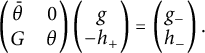$$ \begin{align*} \begin{pmatrix} \bar\theta & 0 \\ G & \theta \end{pmatrix} \begin{pmatrix} g \\ -h_+ \end{pmatrix}= \begin{pmatrix} g_{-} \\ h_- \end{pmatrix}. \end{align*} $$

Analogous relation holds also for $f_1$ , so

$$ \begin{align*} \begin{pmatrix} \bar\theta & 0 \\ G & \theta \end{pmatrix} \begin{pmatrix} g & f_ 1\\ -h_+ & f_2 \end{pmatrix}= \begin{pmatrix} g_{-} & f_{1-} \\ h_- & f_{2-} \end{pmatrix} \end{align*} $$

with $f_2\in H^2$ , $f_{1-},f_{2-}\in H^2_{-}$ . Calculating the determinants on both sides, we get

$$ \begin{align*} gf_2+h_+f_1=g_{-}f_{2-}-h_-f_{1-}. \end{align*} $$

Note that the left-hand side is an element of $H^1$ and the right-hand side is an element of $\overline {zH^1}$ . Thus, both have to be $0$ and it follows that $h_+=\frac {gf_2}{f_1}$ , with $f_1(0)\neq 0$ , so $h_+$ must vanish at $0,$ whenever $g(0)=0$ , i.e., for all $g=H_{\bar z}^{A_G^{\theta }}$ . So (3) follows.

As a consequence of Propositions 7.9 and 7.10 and Theorem 7.1, we can now state the following.

Remark 7.13 We recover in Theorem 7.12 some results obtained, in a different way, in [Reference O’Loughlin27, Section 4], namely that $\ker A_G^{\theta }$ is nearly $\bar z$ -invariant (w.r.t. ${K^2_{\theta }}$ ) if there exists $f_1\in \ker A_G^{\theta }$ with $f_1(0)\neq 0$ , and $\ker A_G^{\theta }$ is nearly $\bar z$ -invariant with defect $1$ if $f(0)=0$ for all $f\in \ker A_G^{\theta }$ . Another interesting result from [Reference O’Loughlin27] is that, in the latter case, if n is the greatest natural number such that $\ker A_G^{\theta }\subset z^nH^2$ , then $z^{-n}\,{\ker A_G^{\theta }}$ is a nearly $S^*$ -invariant subspace. Again, we can obtain this result differently, by observing that

(7.28) $$ \begin{align} z^{-n}\,{\ker A_G^{\theta}}=\ker A_{Gz^n,} \end{align} $$

where not all functions in $\ker A_{Gz^n}$ vanish at $0$ , so by Proposition 7.10, it is nearly $\bar z$ -invariant (w.r.t. ${K^2_{\theta }}$ ). To prove (7.28), take $f\in \ker A_G^{\theta }\subset {K^2_{\theta }}\cap z^n H^2$ , then for some $h_+\in H^2$ , $h_-\in H^2_-$ , we have $Gf=h_-+\theta h_+$ . Thus $(Gz^n)(z^{-n}f)=h_-+\theta h_+$ , so $f=z^n (z^{-n}f)$ with $z^{-n}f \in \ker A_{Gz^n}^{\theta }$ . For the reverse inclusion, note that, if $ (Gz^n)f=h_-+\theta h_+$ , then $G(z^nf)=h_-+\theta h_+$ and $z^nf\in \ker A_G^{\theta }$ , so $z^n \ker A_{Gz^n}^{\theta }\subset \ker A_G^{\theta }$ .

We now compare the decomposition obtained in Example 5.2 with (7.26). We can assume that $G\in {K^2_{\theta }}$ , and $\ker A_G^{\theta }=\gamma {K^2_{\beta }}$ with $\beta <\theta $ , $\gamma =\theta /\beta $ , $\gamma (0)=0$ , $\beta <G^i$ (inner part of G). So, by Theorem 7.12, $\ker A_G^{\theta }$ is nearly $\bar z$ -invariant with defect $1$ and ${K^2_{\theta }}$ -invariant for $M_{\bar z}$ , and we have

$$ \begin{align*} \ker A_G^{\theta}=(\ker A_G^{\theta})_{\bar z} \oplus [P_{\ker A_G^{\theta}}(zA_{\bar G}^{\theta} \tilde k_0^{\theta})], \end{align*} $$

where $P_{\ker A_G^{\theta }}=P_{\gamma {K^2_{\beta }}}=\gamma P_{\beta } \bar \gamma P^+$ . One can see that

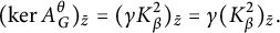$$ \begin{align*} (\ker A_G^{\theta})_{\bar z}=(\gamma {K^2_{\beta}})_{\bar z}=\gamma({K^2_{\beta}})_{\bar z}.\ \end{align*} $$

It is left to show that $[P_{\ker A_G^{\theta }}(zA_{\bar G}^{\theta } \tilde k_0^{\theta })]=[\gamma k_0^{\beta }]$ . Indeed, we have

(7.29) $$ \begin{align} P_{\gamma {K^2_{\beta}}}(zA_{\bar G}^{\theta} \tilde k_0^{\theta})=\gamma P_{\beta} \bar\gamma (zA_{\bar G}^{\theta} \tilde k_0^{\theta})=\gamma P_{\beta} \bar\gamma\theta\bar G, \end{align} $$

because

$$ \begin{align*} A_{\bar G}^{\theta} \tilde k_0^{\theta}=P_{\theta}(\bar G\bar z(\theta-\theta(0)))=P_{\theta}(\bar G\bar z\theta)-P_{\theta}(\bar G\bar z\theta(0))=C_{\theta} G=\theta\bar z\bar G. \end{align*} $$

Hence, from (7.29),

$$ \begin{align*} P_{\gamma {K^2_{\beta}}}(zA_{\bar G}^{\theta} \tilde k_0^{\theta})=\gamma P_{\beta} (\bar\gamma \theta \bar G)=\gamma P_{\beta} (\beta\bar G), \end{align*} $$

where $\beta \bar G\in \overline {H^2}$ , because $\beta $ divides the inner factor $G^i$ . Thus $P_{\beta }(\beta \bar G)=c\in \mathbb {C}$ and $\gamma P_{\beta }(\beta \bar G)=c\gamma k_0^{\beta }$ .

Note that the dichotomy of Theorem 7.12 does not extend to other cases with $\beta \neq z$ , as we show in the following simple example where both $M_G^{\prime }(\bar \beta )$ and $M_G^{\prime \prime }(\bar \beta )$ are different from $\{0\}$ .

Example 7.14 Let $G=z^3$ , $\theta =z^4$ . Then $\ker A_G^{\theta }=zK^2_{z^3}$ so, for $X=\bar z^2$ , the decomposition (7.6) has the form

$$ \begin{align*} \ker A_G^{\theta}= (\ker A_G^{\theta})_{\bar z^2}\oplus M_G^{\prime}(\bar z^2) \oplus M_G^{\prime\prime}(\bar z^2)= [z^3] \oplus [z^2] \oplus [z]. \end{align*} $$

One can also study the z-invariance properties of kernels of truncated Toeplitz operators and obtain the decomposition given in Theorem 7.5 with $\beta =z$ , using Theorem 7.12 and Corollary 7.8.

Theorem 7.15 Let $\theta $ be an inner function and $G\in L^{\infty }$ . We have either

(7.30) $$ \begin{align} \ker A_G^{\theta}=(\ker A_G^{\theta})_z\oplus [P_{\ker A_G^{\theta}}\tilde k_0^{\theta}], \end{align} $$

where the second term in the orthogonal sum corresponds to $ M_G^{\prime \prime }(\bar z)$ in Theorem 7.1, or

(7.31) $$ \begin{align} \ker A_G^{\theta}=(\ker A_G^{\theta})_z\oplus [P_{\ker A_G^{\theta}}(zA_{\bar G}^{\theta}k_0^{\theta})], \end{align} $$

where the second term in the orthogonal sum corresponds to $ M_G^{\prime }(z)$ in Theorem 7.1.

Proof The equivalence between (1) and (2) is a direct consequence of the previous results.

By Theorem 7.11, (2) is equivalent to the fact that, for all $ f\in \ker A_G^{\theta }$ such that $ f(0)=0$ , the first equality holds and

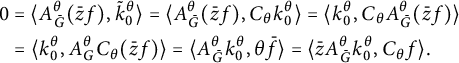$$ \begin{align*} \begin{aligned} 0&=\langle A_{\bar G}^{\theta}(\bar z f),\tilde k_0^{\theta}\rangle= \langle A_{\bar G}^{\theta}(\bar z f),C_{\theta} k_0^{\theta}\rangle =\langle k_0^{\theta},C_{\theta} A_{\bar G}^{\theta}(\bar z f)\rangle\\&= \langle k_0^{\theta},A_G^{\theta} C_{\theta} (\bar z f)\rangle =\langle A_{\bar G}^{\theta}k_0^{\theta},\theta\bar f\rangle = \langle \bar z A_{\bar G}^{\theta}k_0^{\theta},C_{\theta} f \rangle. \end{aligned} \end{align*} $$

For $\tilde f=C_{\theta } f$ , we have, thus, that the above is equivalent to $\langle \bar z A_{\bar G}^{\theta }, \tilde f\rangle =0$ for all $\tilde f\in \ker A_G^{\theta }$ , $(C_{\theta } \tilde f)(0)=0$ . Hence (2) $\Leftrightarrow $ (3).

Now we show that (3) $\Leftrightarrow $ (4). Note that, for $ f$ such as in (3), we have

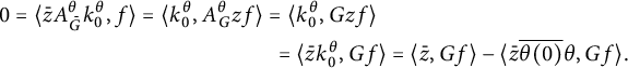$$ \begin{align*} 0=\langle \bar z A_{\bar G}^{\theta}k_0^{\theta}, f \rangle &= \langle k_0^{\theta}, A_G^{\theta} z f \rangle = \langle k_0^{\theta}, Gz f \rangle \\ &\qquad\qquad\qquad = \langle \bar z k_0^{\theta}, G f \rangle = \langle \bar z, G f \rangle - \langle \bar z \overline{\theta(0)}\theta, G f \rangle. \end{align*} $$

Since $ f\in \ker A_G^{\theta }$ , we have that $G f=P^-(G f)+\theta P^+\bar \theta (G f)$ , so the previous equality is equivalent to

$$ \begin{align*} \begin{aligned} 0=&\langle \bar z, P^-G f\rangle - \overline{\theta(0)} \langle \bar z \theta, P^-G f\rangle-\overline{\theta(0)}\langle \bar z \theta, \theta P^+\bar\theta G f\rangle \\ =& \langle \bar z, P^-G f\rangle - \overline{\theta(0)} \langle P^-\bar z \theta, P^-G f\rangle\\ =& \langle \bar z, P^-G f\rangle - \overline{\theta(0)}\theta(0) \langle \bar z, P^-G f\rangle\\=&(1- |{\theta(0)}|^2)\langle \bar z, P^-G f\rangle. \end{aligned} \end{align*} $$

This is equivalent to

$$ \begin{align*}\langle \bar z, P^-Gf\rangle=0,\end{align*} $$

i.e., $P^-G f\in \bar z H_-^2.$

Analogously, we have the following.