


Impact Statement
The primary novel component of this work is that a value of information calculation has been integrated with a partial pooling degradation model, relating information from inspection data across multiple locations. In addition, a Bayesian imputation model (of missing data) was used to estimate the prior damage model. Inspections of engineering structures typically consist of indirect measurements of some complex degradation process, sometimes in challenging environmental conditions. Even when state of the art technologies are employed, the information that they provide is imperfect. Improved probabilistic quantification of inter-dependencies may contribute to the development of risk-optimal inspection and maintenance planning. This is expected to be of particular benefit to ageing structures, associated with limited, incomplete, and lost information.
1. Introduction
1.1. Structural integrity management
Structural integrity management is defined as a structure’s ability to function “effectively” and “efficiently” (Health and Safety Executive, 2009). This joint optimization of safety and economy is a basis for selecting appropriate investments for in-service structures. Since all structures degrade or become damaged to some extent, there may be points in time when it is worthwhile investing in activities that reduce the risk of failure. Identifying where, when and how to inspect (or more generally, to collect information) is an on-going challenge to engineers.
Fundamentally, this requires a mechanism for integrating information from an inspection with existing models of structural condition. There is also the requirement for a means of determining whether or not the expected utility of an inspection exceeds its expected cost, that is whether or not the inspection is expected to be worthwhile. As outlined in this paper, Bayesian inference provides the mathematical basis for achieving this.
1.2. Epistemic uncertainty
In Kiureghian and Ditlevsen (Reference Kiureghian and Ditlevsen2009) various uncertainties that should be considered in structural engineering are outlined. The authors identify that contributions from epistemic (statistical uncertainty due to quality and availability of information) and aleatory (associated with inherent variability) uncertainty can be treated similarly, and this can be achieved using Bayesian methods, where both are represented in the posterior distribution. Probabilistic methods in engineering have historically focused on aleatory uncertainty and various Bayesian methods have been proposed to also account for epistemic uncertainty (Sankararaman and Mahadevan, Reference Sankararaman and Mahadevan2013; Nannapaneni and Mahadevan, Reference Nannapaneni and Mahadevan2016). The influence of epistemic uncertainty will be largest when only small amounts of data are available. In such cases, when neglecting epistemic uncertainty, engineers will overestimate the precision of their models, which can lead to ineffective risk management. Engineering structures are often associated with the absence of large amounts of data and the presence of subject matter knowledge DNVGL (2017c). This is often cited as the reason that quantitative risk-based inspection (RBI) is infeasible in practice (API, 2016; DNVGL, 2017b). Alternatively, this can be considered a reason that structural engineering is well suited to Bayesian methods (Ang and Tang, Reference Ang and Tang2007). Consequently Bayesian methods have been proposed for managing uncertainty in this context for many decades (Tang, Reference Tang1973). Incorporating epistemic uncertainty is more challenging using other methods. For instance, maximum likelihood estimation is primarily concerned with obtaining point estimates of parameters, although with sufficient data the variation can also be estimated (Faber, Reference Faber2012).
1.3. System effects
Inspection planning of systems of components within a structure (or systems of multiple structures) should consider possible dependencies between individual components (Straub and Faber, Reference Straub and Faber2004). Information (such as detection of the presence or absence of damage) at one location should inform estimates of the condition of other locations (Straub and Faber, Reference Straub and Faber2005). This concept is intuitive, but incorporating this effect in a quantitative inspection plan requires models capable of characterizing this dependency. In this paper, partial pooling of information between locations using multilevel Bayesian models, as detailed in Section 3, is proposed as a solution to this challenge. Note that for the purposes of this paper, a multilevel model is considered to be a more general form of a hierarchical model and is used interchangeably with partial pooling model. In Section 4, it is demonstrated how the results of such a model can be integrated with a decision analysis for evaluating prospective inspection options.
Sources of variation in degradation rates are expected to differ between equipment that is manufactured at scale through more established or controlled processes, and structural systems, which may be comprised of less common arrangements. In this paper, it is proposed that a binary classification of a structure or structural component as being either unique, or nominally identical to others in a population is an simplification that can be overcome. This is discussed in more detail in Section 2.
Note that there are also system effects in consequence modeling (Straub and Faber, Reference Straub and Faber2004). For instance, the expected cost of failure of a structural element may be less for structures designed with redundancy. Additionally, the cost of multiple failures may not increase linearly. The work presented in this paper focuses on modeling failure probability and not failure consequences. However, Bayesian methods of quantifying uncertainty are expected to be equally valid for estimating failure consequences, although the details will be conditional on the preferences of the asset operator (and other stakeholders), which are generally not publicly available. Conversely, certain failure mechanisms are common across welded steel structures and components, and can therefore be discussed more generally.
2. Risk Based Inspection
2.1. Historical developments
RBI procedures have been developed for many industries, including petrochemical plant (Wintle et al., Reference Wintle, Kenzie, Amphlett and Smalley2001; API, 2008; API, 2016), ship hulls (Lloyd’s Register, 2017), offshore structures (Health and Safety Executive, 2009; DNVGL, 2015; Bureau Veritas, 2017; Guédé, Reference Guédé2018), and offshore topsides equipment (DNVGL, 2017b). Despite the variation in application, these procedures share many common features. Specifically, they are all concerned with a risk optimal allocation of resources based on some evaluation of the probability and consequence of failure. However, these high-level principles allow for significant variation in their application, and catastrophic failures have been recorded at sites with RBI systems in place. A review of two such incidents Clarke (Reference Clarke2016) highlighted (among other issues) that procedures which prioritize inspections to be completed within a specified time-frame are “doomed to failure.” Rather, inspections that are shown to be required should be completed. In addition, this report also recommended that any decisions which results from an RBI assessment should be auditable and accountable.
Some industries make direct use of large datasets to infer expected probabilities of failure. In API (2008), the idea of a generic failure frequency (that summarizes failures from large numbers of components, which have been assumed to belong to a single population) is central to the recommended RBI practices. In the case of structures, this is generally not considered suitable as the variation between different structures is considered too great (Thoft-Christensen and Baker, Reference Thoft-Christensen and Baker1982; Straub, Reference Straub2004). While structures may vary more than mass manufactured process equipment, there will be some degree of commonality that they share. Conversely, no two mass manufactured components degrade in a completely identical manner and so they will also exhibit some variation. The modeling approach detailed in Section 3 is capable of accounting for this on a continuous scale.
A method originally proposed in Madsen (Reference Madsen1987) and still used in conjunction with structural reliability analysis (Ditlevsen and Madsen, Reference Ditlevsen and Madsen2007) is presented in Equations (1) and (2). It shows scheduling of inspections before a probability of failure, $ \Pr \left(\mathrm{Fail}\right) $
, (due to some active degradation mechanism) exceeds a threshold. Updating of
$ \Pr \left(\mathrm{Fail}\right) $
, (due to some active degradation mechanism) exceeds a threshold. Updating of $ \Pr \left(\mathrm{Fail}\right) $
following inspections assumes that no damage is detected. Here
$ \Pr \left(\mathrm{Fail}\right) $
following inspections assumes that no damage is detected. Here $ d $
represents the extent of damage,
$ d $
represents the extent of damage, $ {d}_C $
is the critical dimensions beyond which failure is predicted and
$ {d}_C $
is the critical dimensions beyond which failure is predicted and $ H $
is the extent of the damage reported by an inspection. This calculation can be completed using methods of structural reliability, or sampling procedures.
$ H $
is the extent of the damage reported by an inspection. This calculation can be completed using methods of structural reliability, or sampling procedures.
 $$ \Pr \left(\mathrm{Fail}\right)=\Pr \left({d}_C\le d\right), $$
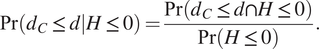 $$ \Pr \left({d}_C\le d|H\le 0\right)=\frac{\Pr \left({d}_C\le d\cap H\le 0\right)}{\Pr \left(H\le 0\right)}. $$
This approach does account for inspection reliability, as fewer inspections are shown to be required when a method with a higher probability of detection (PoD) is used. However, it needs to be combined with some decision rule (such as any detected damage will be immediately repaired). A more flexible approach may consider the prior likelihood of whether damage will be detected, and use this to help quantify the value of the data that each inspection will provide.
2.2. Quantitative methods (Bayesian decision analysis)
Inspection data, $ z $
, of various type and quality may be available to engineers, and can be related to uncertain parameters of interest,
$ z $
, of various type and quality may be available to engineers, and can be related to uncertain parameters of interest, $ \theta $
, using a probabilistic model,
$ \theta $
, using a probabilistic model, $ f\left(z|\theta \right) $
. This can be used to update a prior model,
$ f\left(z|\theta \right) $
. This can be used to update a prior model, $ \pi \left(\theta \right) $
, to obtain a posterior model,
$ \pi \left(\theta \right) $
, to obtain a posterior model, $ \pi \left(\theta |z\right) $
using Bayes’ theorem, as shown in Equation (3). Understanding the requirements for information collection requires these probabilistic models to be combined with a decision analysis (Jaynes, Reference Jaynes2003) and this principle has been acknowledged in the context of statistical experimental design for decades (Berger, Reference Berger1985). Quantification of the expected value of information (VoI) is a special application of Bayesian decision analysis. It is sometimes referred to as preposterior decision analysis (Jordaan, Reference Jordaan2005), and sometimes as multistage decision-making under uncertainty (Gelman et al., Reference Gelman, Carlin, Stern and Rubin2014). Its application to structural integrity management has been investigated extensively in recent years (Pozzi and Der Kiureghian, Reference Pozzi and Der Kiureghian2011; Straub, Reference Straub2014; Di Francesco et al., Reference Di Francesco, Chryssanthopoulos, Havbro Faber and Bharadwaj2021).
$ \pi \left(\theta |z\right) $
using Bayes’ theorem, as shown in Equation (3). Understanding the requirements for information collection requires these probabilistic models to be combined with a decision analysis (Jaynes, Reference Jaynes2003) and this principle has been acknowledged in the context of statistical experimental design for decades (Berger, Reference Berger1985). Quantification of the expected value of information (VoI) is a special application of Bayesian decision analysis. It is sometimes referred to as preposterior decision analysis (Jordaan, Reference Jordaan2005), and sometimes as multistage decision-making under uncertainty (Gelman et al., Reference Gelman, Carlin, Stern and Rubin2014). Its application to structural integrity management has been investigated extensively in recent years (Pozzi and Der Kiureghian, Reference Pozzi and Der Kiureghian2011; Straub, Reference Straub2014; Di Francesco et al., Reference Di Francesco, Chryssanthopoulos, Havbro Faber and Bharadwaj2021).
 $$ \pi \left(\theta |z\right)\propto \pi \left(\theta \right)\cdot f\left(z|\theta \right). $$
A decision tree representation of the question of how, and to what extent, an inspection is expected to benefit risk management is shown in Figure 1. Here, available inspection options, $ E $
, can provide additional data,
$ E $
, can provide additional data, $ Z $
(unless the option not to inspect is selected). Following this, risk mitigation options,
$ Z $
(unless the option not to inspect is selected). Following this, risk mitigation options, $ A $
(again, including the option to do nothing) are available. These decisions will influence the parameters describing structural condition,
$ A $
(again, including the option to do nothing) are available. These decisions will influence the parameters describing structural condition, $ \Theta $
. The utility of this outcome is a function of each of these outcomes,
$ \Theta $
. The utility of this outcome is a function of each of these outcomes, $ u\left[e,a,\pi \left(\theta |z\right)\right] $
.
$ u\left[e,a,\pi \left(\theta |z\right)\right] $
.
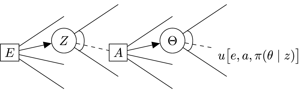
Figure 1. Decision tree representation of inspection evaluation.
The joint optimization over the two decision nodes (shown as squares in Figure 1) is presented in Equation (4). It simply states that the optimal inspection, $ {e}^{\ast } $
, and risk mitigation,
$ {e}^{\ast } $
, and risk mitigation, $ {a}^{\ast } $
, are those associated with the expected maximum utility (or minimum cost).
$ {a}^{\ast } $
, are those associated with the expected maximum utility (or minimum cost).
 $$ {e}^{\ast },{a}^{\ast }=\mathit{\arg}\underset{e\in E,a\in A}{\max }u\left[e,a,\pi \left(\theta |z\right)\right]. $$
The expected value of any given inspection, $ {\mathrm{VoI}}_{e_i} $
, is the difference in expected utility with,
$ {\mathrm{VoI}}_{e_i} $
, is the difference in expected utility with, $ u[{e}_i,{a}_{e_i}^{\ast },\pi \left(\theta |z\right)] $
, and without,
$ u[{e}_i,{a}_{e_i}^{\ast },\pi \left(\theta |z\right)] $
, and without, $ u\left[{a}^{\ast },\pi \left(\theta \right)\right] $
, the information it provides, see Equation (5). As indicated by the multiple branches in Figure 1, this calculation requires integration over various possible outcomes. For instance, a continuum of possible inspection results
$ u\left[{a}^{\ast },\pi \left(\theta \right)\right] $
, the information it provides, see Equation (5). As indicated by the multiple branches in Figure 1, this calculation requires integration over various possible outcomes. For instance, a continuum of possible inspection results $ z\in Z $
can be accounted for by sampling from a prior probabilistic model and averaging the subsequent expected costs. This method has been used in Section 4.
$ z\in Z $
can be accounted for by sampling from a prior probabilistic model and averaging the subsequent expected costs. This method has been used in Section 4.
 $$ {\mathrm{VoI}}_{e_i}=u\left[{e}_i,{a}_{e_i}^{\ast },\pi \left(\theta |z\right)\right]-u\left[{a}^{\ast },\pi \left(\theta \right)\right]. $$
VoI analysis is capable of identifying risk-optimal inspection strategy for nonintuitive decision problems. In other instances, the risk-optimal solution may be self-evident to engineers, however, even in such cases a formal, reproducible analysis will make it easier to revise or audit.
2.3. Inspection quality
The American Petroleum Institute (API) has developed RBI guidance for petrochemical industry (API, 2008; , 2016). These documents acknowledge that the quality of an inspection determines the extent to which uncertainty can be reduced, and that this can directly influence an estimated probability of failure, obtained by a structural reliability analysis. Bayesian analysis is listed as a method of accounting for Inspection Effectiveness, but the API procedures provide a qualitative ranking method. An inspection is assigned a rank on a scale of A (representing a highly effective inspection) to E (representing an ineffective inspection). A damage factor, which is used to obtain a semi-quantitative estimate of the probability of failure, is reduced based on the inspection effectiveness rank. A similar qualitative categorization is provided in an RBI recommended practice for offshore topsides equipment (DNVGL, 2017b). Such heuristics allow for the intuitive concept of inspection quality to be accounted for, albeit in a possibly imprecise way.
Quantifying the expected value of an inspection requires mathematical characterization of the information provided and a model relating it to the parameters of interest (Faber, Reference Faber2000; Straub, Reference Straub2004; Straub et al., Reference Straub, Sørensen, Goyet and Faber2006; Di Francesco et al., Reference Di Francesco, Chryssanthopoulos, Havbro Faber and Bharadwaj2021). Assuming perfect information results in overestimation of the VoI of inspection activities. The mechanism for describing how probabilistic models are updated based on new information (such as inspection) is Bayes’ theorem, as shown in Equation (3). Here, the prior models of parameters, $ \pi \left(\theta \right) $
are combined with a likelihood function,
$ \pi \left(\theta \right) $
are combined with a likelihood function, $ f\left(z|\theta \right) $
(which describes the imperfect features of the inspection data,
$ f\left(z|\theta \right) $
(which describes the imperfect features of the inspection data, $ z $
), to generate an updated, posterior model,
$ z $
), to generate an updated, posterior model, $ \pi \left(\theta |z\right) $
. Reducing uncertainty in probabilistic models of damage allows for better informed decisions and improved risk management.
$ \pi \left(\theta |z\right) $
. Reducing uncertainty in probabilistic models of damage allows for better informed decisions and improved risk management.
3. Modeling Imperfect Inspection Data
3.1. Imperfect data
The value of an inspection is dependent on (among other factors) the quality of the data that will collected. Data from a more precise and reliable inspection will reduce uncertainty to a greater extent. These qualities should be reflected in its expected value. A detailed review of approaches to mathematically characterize such features of an imperfect inspection is provided in Di Francesco et al. (Reference Di Francesco, Chryssanthopoulos, Havbro Faber and Bharadwaj2021). In Ali et al. (Reference Ali, Qin and Faber2020), an alternative categorization of imperfect information (based on that proposed in Nielsen et al. (Reference Nielsen, Glavind, Qin and Faber2019) is also presented in the context of VoI.
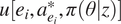
As identified in Di Francesco et al. (Reference Di Francesco, Chryssanthopoulos, Havbro Faber and Bharadwaj2021), the precision, bias and reliability of inspection data can be modeled as shown in Equations (6) and (7). Here, a measurement of the extent of damage, $ {d}_{\mathrm{meas}} $
, is normally distributed with a mean equal to the true extent,
$ {d}_{\mathrm{meas}} $
, is normally distributed with a mean equal to the true extent, $ d $
plus any bias,
$ d $
plus any bias, $ \delta $
, with some sizing variance,
$ \delta $
, with some sizing variance, $ \varepsilon $
. This model is shown graphically in Figure 2. The probability of this damage being detected by the inspection can be modeled using a logistic regression, where
$ \varepsilon $
. This model is shown graphically in Figure 2. The probability of this damage being detected by the inspection can be modeled using a logistic regression, where $ \alpha $
and
$ \alpha $
and $ \gamma $
represent a linear regression co-efficient and intercept, respectively, on the log-odds scale (Health and Safety Executive, 2006). Such a model is presented in Figure 3.
$ \gamma $
represent a linear regression co-efficient and intercept, respectively, on the log-odds scale (Health and Safety Executive, 2006). Such a model is presented in Figure 3.
 $$ {d}_{\mathrm{meas}}\sim N\left(d+\delta, \varepsilon \right), $$
 $$ \mathrm{PoD}=\frac{\exp -\left(\alpha +\gamma \cdot \mathit{\ln}(d)\right)}{1+\exp -\left(\alpha +\gamma \cdot \mathit{\ln}(d)\right)}. $$
Figure 2. Gaussian sizing accuracy model.
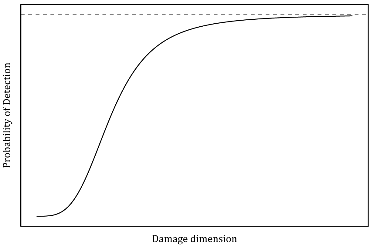
Figure 3. Logistic regression probability of detection (PoD) model.
3.2. Incomplete (missing) data
Engineers may often be required to work with incomplete datasets, which is less frequently accounted for in existing VoI scientific literature. In Qin et al. (Reference Qin, Zhou and Zhang2015), cases of an inspection not detecting damage are considered to be missing data. In Di Francesco et al. (Reference Di Francesco, Chryssanthopoulos, Havbro Faber and Bharadwaj2021), such instances are treated as information in a Bayesian updating procedure. Rather, missing data represents the absence of information and some examples of this are listed below:
-
• Operational constraints: Some part of an inspection not completed, perhaps due to time constraints, or unsafe weather conditions.
-
• Inspection technology not operating: Excursions from normal operating conditions, or mechanical damage, could cause electronic components to stop functioning.
-
• Lost data: An analysis may be considering historical inspection and maintenance data. If these data were recorded before a data management system, or when it was operated by a previous asset owner, then it may be at least partially lost.
The standard approach for analysis of incomplete datasets is to disregard cases with one or more missing data points. This is known as a complete case analysis, and is only appropriate when the reduced dataset has not been biased by the removal of incomplete cases. An alternative approach is imputation of missing data, which uses available information to estimate the missing values.
As outlined in Gelman et al. (Reference Gelman, Hill and Vehtari2020) and McElreath (Reference McElreath2020), whether the data are missing at random will determine how it should be imputed. For instance, if there is a causal link between the value of the data and its missingness status then this should be accounted for in a model.
The Bayesian framework is well suited to probabilistic imputation of missing data. Missing values can be inferred in the same way as other (unobserved) model parameters such that probabilistic estimates are identified, which are consistent with the other data, in the context of the specified model.
3.3. Multilevel modeling approach to quantifying system effects
In Straub and Faber (Reference Straub and Faber2004), the authors suggest that the condition of multiple, so-called hot spots, Footnote 1 on a structure should somehow be related. In Straub and Faber (Reference Straub and Faber2005), it is proposed that this can be achieved through a co-variance matrix that describes common factors between locations. In practice, some of the underlying factors for these dependencies may not be intuitive, and even for those that are identified it is unlikely that the specific data required will be available for estimating correlation co-efficients or copula parameters. The solution proposed in this paper is to use multilevel Bayesian models Gelman (Reference Gelman2006) to partially pool information between locations.
When fitting a conventional Bayesian model, a set of parameters, $ \theta $
, are estimated based on some measurements,
$ \theta $
, are estimated based on some measurements, $ z $
(described using a likelihood function), and prior models,
$ z $
(described using a likelihood function), and prior models, $ \pi \left(\theta \right) $
. Often, engineers must incorporate data from different sources. In this context, information from an inspection at one location can help inform models of structural condition at another location. When differing locations are modeled as a discrete heterogeneity in inspection data, Bayesian multilevel models can be used to estimate degradation rates, as detailed in this Section.
$ \pi \left(\theta \right) $
. Often, engineers must incorporate data from different sources. In this context, information from an inspection at one location can help inform models of structural condition at another location. When differing locations are modeled as a discrete heterogeneity in inspection data, Bayesian multilevel models can be used to estimate degradation rates, as detailed in this Section.
When combining data from multiple sources, engineers may choose to create a single (fully pooled) population and use this to fit a model. This approach neglects any variation between the datasets, and failing to account for this will introduce bias to any predictions. For instance, if the condition of two hot spots differs significantly, then a model which fully pools data from inspections at these locations will result in some average, which may not accurately predict the condition of either. This can be addressed by fitting separate models to each dataset, but could introduce excessive variance to the predictions, since the models are now being estimated based on less evidence. The optimal solution will be somewhere in between these two extremes of dependency and can be realized by fitting a Bayesian multilevel model (Gelman, Reference Gelman2006; Gelman and Hill, Reference Gelman and Hill2007).
A graphical representation of a partial pooling Bayesian model is shown in Figure 4. Here, a separate set of parameters are estimated for each group, but population level priors (which control the extent of pooling for each parameter) are also estimated from the data (and hyperpriors). Further discussion on the extent of pooling from a multilevel model is presented in Section 4.

Figure 4. Structure of a multilevel (partial pooling) Bayesian model for estimating parameters, $ \theta $
, from data, z, priors,
$ \theta $
, from data, z, priors, $ {\theta}_{\mathrm{pr}} $
, and hyperpriors,
$ {\theta}_{\mathrm{pr}} $
, and hyperpriors, $ {\hat{\theta}}_{\mathrm{pr}} $
.
$ {\hat{\theta}}_{\mathrm{pr}} $
.
As demonstrated in Di Francesco et al. (Reference Di Francesco, Chryssanthopoulos, Havbro Faber and Bharadwaj2020), Bayesian multilevel models can be used to improve estimates of structural condition at locations remote to where an inspection has been completed. If there is some commonality between the condition of a location being inspected and the condition of another location of interest, then engineers can learn indirectly something about the latter, by inspecting the former. This has the potential to increase the value of the inspection activity, since the same data is now being used to update models at additional locations.
In a different setting, this approach has also been demonstrated for combining evidence from different test datasets to estimate the parameters of a fatigue crack growth model (Di Francesco et al., Reference Di Francesco, Chryssanthopoulos, Havbro Faber and Bharadwaj2020). The benefit of allowing for possible variability between tests (which were completed in different labs, on different steels) was quantified using out of sample predictive performance criteria.
The Bayesian models presented in this work have been fit using Markov Chain Monte Carlo (MCMC) sampling. The suitability of Hamiltonian Monte Carlo (a modern MCMC algorithm) as a procedure for sampling from multilevel models is demonstrated in Betancourt and Girolami (Reference Betancourt and Girolami2015). The calculations presented in this paper make use of the no u-turn implementation of Hamiltonian Monte Carlo (Hoffman and Gelman, Reference Hoffman and Gelman2014) in the probabilistic programming language, Stan (Carpenter et al., Reference Carpenter, Gelman, Hoffman, Lee, Goodrich, Betancourt, Brubaker, Guo, Li and Riddell2017).
4. Example Application: Inspecting for Corrosion Damage
4.1. Problem overview
Corrosion is considered as the degradation mechanism in the example in this section, primarily because new data from inspections are typically used to update estimates of degradation rate (Health and Safety Executive, 2002). Estimation of corrosion rates is a statistical challenge. Unlike traditional alternatives, Bayesian methods can be used to obtain estimates from small datasets, accounting for imperfect features of the data available. A simple model of corrosion rate, $ \beta $
, using the inspection data,
$ \beta $
, using the inspection data, $ {d}_i $
is proposed in Equations (8) and (9).
$ {d}_i $
is proposed in Equations (8) and (9).
 $$ {\beta}_i=\frac{d_{\mathrm{meas}}^{t={T}_2}-{d}_{\mathrm{meas}}^{t={T}_1}}{T_2-{T}_1}, $$
 $$ \beta \sim N\left({\mu}_{\beta },{\sigma}_{\beta}\right). $$
The true corrosion rate (in mm year−1) has been assigned as being normally distributed with a mean value of $ 1 $
and a standard deviation of 0.2. In the case of the first inspection measurements are unbiased (
$ 1 $
and a standard deviation of 0.2. In the case of the first inspection measurements are unbiased ( $ \delta =0 $
) with sizing accuracy parameter,
$ \delta =0 $
) with sizing accuracy parameter, $ \varepsilon =0.5 $
(see Equations (6) and (7)). The second inspection is more precise, with
$ \varepsilon =0.5 $
(see Equations (6) and (7)). The second inspection is more precise, with $ \delta =0 $
and
$ \delta =0 $
and $ \varepsilon =0.3 $
.
$ \varepsilon =0.3 $
.
The challenge of corrosion rate estimation is extended to consider the additional challenge multiple locations. Thirteen separate sites of corrosion are considered, with identifiers 1–13. Sites 1–10 were measured at location $ A $
and sites 11–13 were measured at location
$ A $
and sites 11–13 were measured at location $ B $
. There may be reasons to expect differing corrosion rates between remote locations, for example, due to variation in the local environment and the performance of any corrosion protection systems. Consequently, combining these data into a single population will result in biased predictions and using separate models (and separate data) will result in additional variance. This will be especially problematic if at least one location has only very limited evidence. A partial pooling model will allow for information to be shared so that measurements can inform predictions at different locations. This principle this could be extended to many more locations, as proposed in Di Francesco et al. (Reference Di Francesco, Chryssanthopoulos, Havbro Faber and Bharadwaj2020) and illustrated in Figure 5.
$ B $
. There may be reasons to expect differing corrosion rates between remote locations, for example, due to variation in the local environment and the performance of any corrosion protection systems. Consequently, combining these data into a single population will result in biased predictions and using separate models (and separate data) will result in additional variance. This will be especially problematic if at least one location has only very limited evidence. A partial pooling model will allow for information to be shared so that measurements can inform predictions at different locations. This principle this could be extended to many more locations, as proposed in Di Francesco et al. (Reference Di Francesco, Chryssanthopoulos, Havbro Faber and Bharadwaj2020) and illustrated in Figure 5.

Figure 5. Representation of dependencies between inspected locations ( $ i $
) and non-inspected locations (
$ i $
) and non-inspected locations ( $ \overline{i} $
) in a partial pooling Bayesian model.
$ \overline{i} $
) in a partial pooling Bayesian model.
The corrosion site with identifier 11 (at location $ B $
) was assumed not to have been measured during the second inspection. Therefore, a probabilistic estimate of the extent of the damage at this time has been imputed, as described in Section 3.
$ B $
) was assumed not to have been measured during the second inspection. Therefore, a probabilistic estimate of the extent of the damage at this time has been imputed, as described in Section 3.
4.2. Prior predictive simulation
Sampling from the prior distributions of a statistical model allows for a graphical representation of the information they contain on a meaningful outcome scale. This approach (known as prior predictive simulation) is advocated for in Gelman et al. (Reference Gelman, Simpson and Betancourt2017), Gabry et al. (Reference Gabry, Simpson, Vehtari, Betancourt and Gelman2019), and McElreath (Reference McElreath2020). This is especially important when parameters undergo some transformation, such as in generalized linear models, whereas the normal likelihood model for corrosion rate is comparatively simple. Nevertheless, prior predictive simulation for the model described by Equations (8)–(11) is shown in Figure 6. This demonstrates that a large range of corrosion rates are considered credible (in advance of conditioning on any inspection data). They are broadly constrained to be of the order of a few mm year−1, and corrosion specialists may be able to provide additional information, when the priors are presented visually in this way.
 $$ {\mu}_{\beta}\sim N\left(\frac{1}{2},3\right), $$
 $$ {\sigma}_{\beta}\sim \exp \left(\frac{1}{3}\right). $$

Figure 6. Prior predictive simulation of corrosion rate.
4.3. Value of information calculation procedure
Figure 7 shows the measurements from location $ B $
, including the missing data which has been imputed using an independent (no pooling) model. Figure 8 shows the data from all sites, including the missing data, which has been imputed using a multilevel (partial pooling) model.
$ B $
, including the missing data which has been imputed using an independent (no pooling) model. Figure 8 shows the data from all sites, including the missing data, which has been imputed using a multilevel (partial pooling) model.

Figure 7. Bayesian estimate of missing data using independent models.

Figure 8. Bayesian estimate of missing data using multilevel (partial pooling) model.
Figure 9 shows the $ \mathrm{1,000} $
samples from the imputed depths at site 11 that have been selected for the VoI analysis. The samples (shown as histograms) are compared with the MCMC samples from the posterior distributions (shown as density plots). These samples represent possible measurements from the proposed inspection of site 11.
$ \mathrm{1,000} $
samples from the imputed depths at site 11 that have been selected for the VoI analysis. The samples (shown as histograms) are compared with the MCMC samples from the posterior distributions (shown as density plots). These samples represent possible measurements from the proposed inspection of site 11.

Figure 9. Samples from the Bayesian imputation models for the missing data site.
In Figure 10, the predictions of corrosion at site 11 from both the independent and partial pooling model are compared. On this scale, it is evident that the uncertainty in this parameter has been reduced by leveraging the information from location $ A $
. However, in both models, it has not been quantified as precisely as the sites which were measured (as shown in Figures 7 and 8). A VoI analysis can be used to quantify the expected value of completing the inspection at the location of the missing data.
$ A $
. However, in both models, it has not been quantified as precisely as the sites which were measured (as shown in Figures 7 and 8). A VoI analysis can be used to quantify the expected value of completing the inspection at the location of the missing data.

Figure 10. Comparison of Bayesian estimates of missing data between two model structures.
As shown in Equation (5), the VoI is the difference between the utility with (posterior expected cost) and without (prior expected cost) the inspection. The expected costs are calculated based on the below decision problem.
All sites of corrosion damage in this simulated example are considered to be axially oriented in a 20-inch, schedule 60-Grade $ B $
(ASME International and American Petroleum Institute, 2012) linepipe. The failure pressure has been taken to be 38.6 MPa. This results in a hoop stress just below the specified minimum yield strength and could represent an overpressure event during normal operation. Considering only loads from internal pressure (and assuming a constant aspect ratio of 10Footnote
2), the modified ASME B31G assessment method (ASME International, 2012) has been used to predict failure. Similar procedures are provided in BSI (2019) and DNVGL (2017a). The failure stress,
$ B $
(ASME International and American Petroleum Institute, 2012) linepipe. The failure pressure has been taken to be 38.6 MPa. This results in a hoop stress just below the specified minimum yield strength and could represent an overpressure event during normal operation. Considering only loads from internal pressure (and assuming a constant aspect ratio of 10Footnote
2), the modified ASME B31G assessment method (ASME International, 2012) has been used to predict failure. Similar procedures are provided in BSI (2019) and DNVGL (2017a). The failure stress, $ {S}_{\mathrm{fail}} $
, is related to the corrosion depth,
$ {S}_{\mathrm{fail}} $
, is related to the corrosion depth, $ d $
, axial extent,
$ d $
, axial extent, $ l $
, normalized axial extent,
$ l $
, normalized axial extent, $ {l}_z $
, and pipeline (outer) diameter,
$ {l}_z $
, and pipeline (outer) diameter, $ D $
, as shown in Equation (12). Here, the flow strength,
$ D $
, as shown in Equation (12). Here, the flow strength, $ {S}_{\mathrm{flow}} $
is equal to the mean of the yield and tensile strength and
$ {S}_{\mathrm{flow}} $
is equal to the mean of the yield and tensile strength and $ M $
is defined in Equations (13) and (14).
$ M $
is defined in Equations (13) and (14).
 $$ {S}_{\mathrm{fail}}={S}_{\mathrm{flow}}\cdot \left[\frac{1-0.85\cdot \frac{d}{t}}{1-0.85\cdot \frac{d}{t}\cdot {M}^{-1}}\right], $$
 $$ M=\left\{\begin{array}{ll}\sqrt{1+0.6275\cdot {l}_z-.003375\cdot {l_z}^2,}& \mathrm{for}\hskip0.5em {l}_z\le 50,\\ {}0.032\cdot {l}_z+3.3,& \mathrm{for}\hskip0.5em {l}_z>50,\end{array}\right. $$
 $$ {l}_z=\frac{l^2}{D\cdot t}. $$
Following the second inspection (and the identification of the apparently high corrosion rates, a repair plan is required for the next year. Prior probabilities of failure for each site are presented in Figure 11. The calculation outlined in this section details how the expected value of completing the inspection at site 11 can be calculated for both independent and partial pooling Bayesian models. As detailed in Section 1, this work does not include detailed cost modeling. For the purposes of this example, normalized values have been assumed, where the cost of each repair is 1.0 and the cost of each failure is 10.0.

Figure 11. Probability of failure for each corrosion site from both model structures.
Differences in the probabilities of failure between the two model structures are primarily due to the differing corrosion rates that have been estimated. As shown in Figure 12, the corrosion rate can be estimated more precisely (with less variance in the probabilistic estimate) at location $ A $
, and this is because more inspection data are available than at location
$ A $
, and this is because more inspection data are available than at location $ B $
. However, both locations can be estimated more precisely by the partial pooling model. The reduced probability mass at the tails in the predictions from the partial pooling model results in extreme corrosion rates being considered less likely. This includes very low corrosion rates, which would have reduced the estimated probability of failure of large damage, and very high corrosion rates, which would have increased the estimated probability of failure of small damage. This effect is evident in Figure 11, and is larger at the sites at location
$ B $
. However, both locations can be estimated more precisely by the partial pooling model. The reduced probability mass at the tails in the predictions from the partial pooling model results in extreme corrosion rates being considered less likely. This includes very low corrosion rates, which would have reduced the estimated probability of failure of large damage, and very high corrosion rates, which would have increased the estimated probability of failure of small damage. This effect is evident in Figure 11, and is larger at the sites at location $ B $
, where there is a greater improvement in the corrosion rate predicted by the two models.
$ B $
, where there is a greater improvement in the corrosion rate predicted by the two models.

Figure 12. Posterior distribution of corrosion rates from each model structure.
As discussed in Section 3, the extent of pooling between locations is not arbitrary. Rather it is determined from the variance parameters of the (population level) priors for the parameters that are to be partially pooled. An example of the posterior distribution of the mean corrosion rate is presented in Figure 13. Here, values approaching 0 would indicate very little variation between the locations and would therefore justify a greater extent of pooling of information between them. Conversely, very large values would be associated with models that exhibit very little pooling.

Figure 13. Posterior distribution of parameter controlling pooling of the mean corrosion rate.
In this example, the two locations have been assumed to share the same corrosion rate, and this have been identified by the model as shown by the posterior distribution in Figure 13. A consequence of this assumption is that the model is expected to identify evidence of commonality, and partially pool estimates of corrosion rates. This model structure is equally valid for examples when “true” corrosion rates differ between locations, although this will result in less pooling.
5. Results
For each sample in Figure 9, the Bayesian models are re-evaluated and a decision analysis is completed. A PoD was estimated, based on the PoD curve defined in Equation (7), with parameter values $ \alpha =-3 $
and
$ \alpha =-3 $
and $ \gamma =5 $
. As shown in Figure 14, these probabilities may appear to be relatively high, but recall that earlier, reduced damage was previously identified at these locations. In cases where the damage was not expected to be detected, reduced corrosion rates were estimated and propagated through the decision analysis.
$ \gamma =5 $
. As shown in Figure 14, these probabilities may appear to be relatively high, but recall that earlier, reduced damage was previously identified at these locations. In cases where the damage was not expected to be detected, reduced corrosion rates were estimated and propagated through the decision analysis.

Figure 14. Histogram of simulated probability of detection (PoD) for each of the samples.
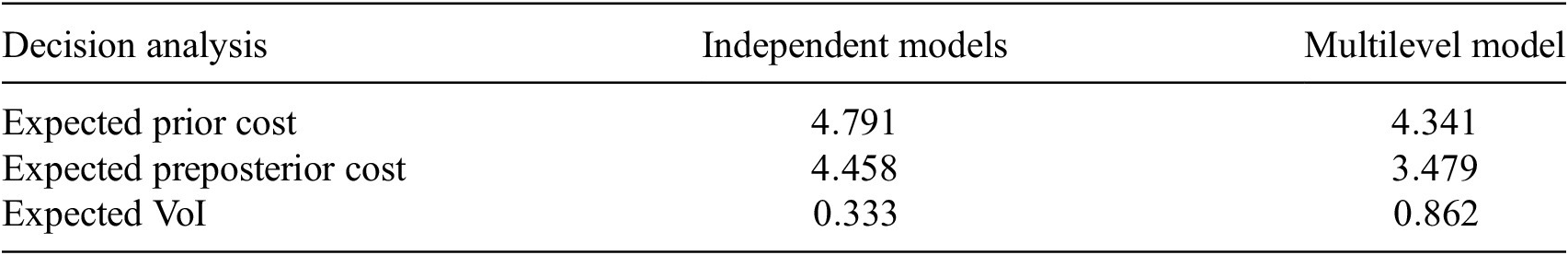
The subsequent preposterior costs are shown in Figure 15, which also includes the difference between the expected value of the prior and preposterior costs (labeled as the expected VoI). These results are also shown in Table 1 as proportions of the cost of a repair. As stated in Section 4.1, the cost of each failure is assumed to be 10 times the cost of each repair, with the repair given a unit cost. Thus, the expected VoI of the additional inspection is estimated to be equal to 33% of the repair cost (for independent models) and circa 86% of the same cost (for the multilevel model).
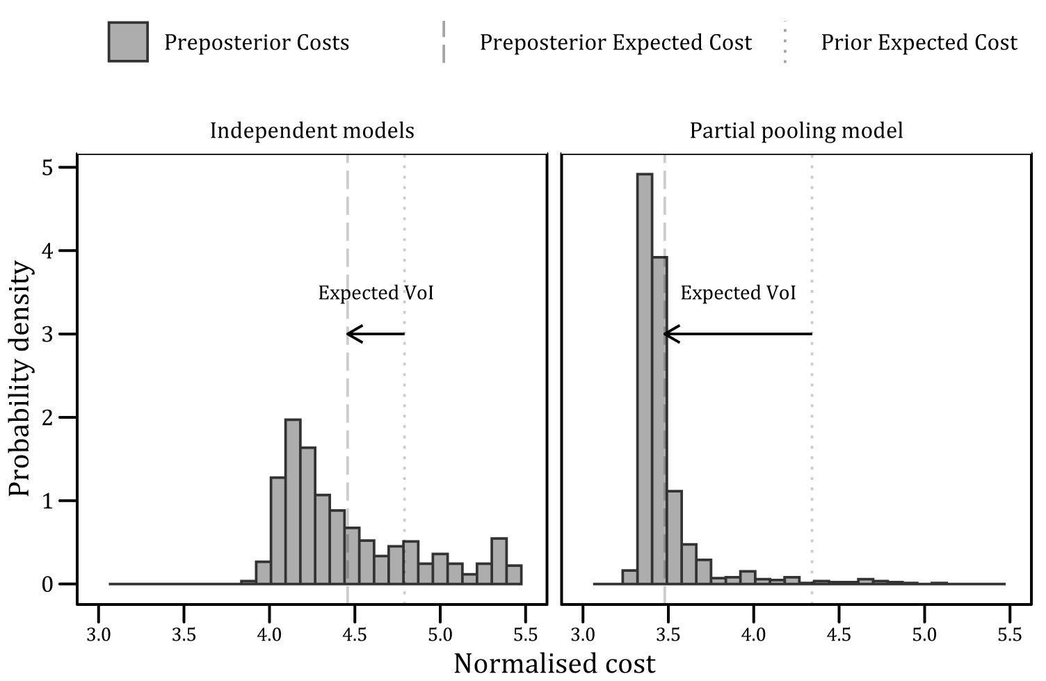
Figure 15. Comparison of expected value of inspection between two model structures.
Table 1. Results from the value of information (VoI) analysis.
6. Discussion
The additional expected value of partially pooled inspection data (shown in Table 1 and Figure 15) is attributed to the wider use of the data (in the context of the multilevel corrosion rate model). However, it is also acknowledged that precise values cannot be generalized since VoI analysis is case-dependent and will vary with new utility functions and structural reliability assessments.
An additional novel feature of the VoI analysis, is that the prior damage model (which is used to generate hypothetical inspection data) has been obtained using a Bayesian imputation model. That is to say, it is a probabilistic model, consistent with available inspection data (of some known precision and reliability) at all other locations.
The simulated corrosion rate did not vary between locations, so the model was expected to identify evidence of similarity and therefore pool estimates, as was shown to be the case in Figures 12 and 13. Further work could be completed to investigate the extent of pooling when there is more variation between locations. When the variation extends to the point that a single underlying model is no longer considered appropriate for all locations, multilevel models are no longer suitable. A full probabilistic analysis of such data could provide quantitative justification for separate models, but this finding could be hidden if outliers are removed, or any other cherry picking of data are completed.
7. Computational Considerations
7.1. Fitting multilevel Bayesian models
Transitioning from conventional Bayesian models to a multilevel structure increases the number of parameters to be estimated significantly. Each parameter being partially pooled is now estimated for each exchangeable group, and a prior is also now inferred from the data. Navigating a higher dimensional probability space will be more challenging for any algorithm and so the efficiency of these models suffer. When using partial pooling models to account for system effects in VoI analysis, these issues are compounded with the existing challenges of computational preposterior decision analysis, described in Straub (Reference Straub2014), Pozzi and Der Kiureghian (Reference Pozzi and Der Kiureghian2011), and Di Francesco et al. (Reference Di Francesco, Chryssanthopoulos, Havbro Faber and Bharadwaj2021).
7.2. Model diagnostics
A comparison of quantitative MCMC diagnostics are shown for each of the models in the example calculation in Section 3. The effective sample size, $ {n}_{\mathrm{eff}} $
and the Gelman–Rubin auto-correlation measure,
$ {n}_{\mathrm{eff}} $
and the Gelman–Rubin auto-correlation measure, $ \hat{R} $
(Gelman et al., Reference Gelman, Carlin, Stern and Rubin2014) are shown in Figures 16 and 17, respectively for each model structure. In Figures 16 and 17, each data point represents an unobserved parameter that the model has estimated. In Figure 18, each data point represents a separate Markov chain.
$ \hat{R} $
(Gelman et al., Reference Gelman, Carlin, Stern and Rubin2014) are shown in Figures 16 and 17, respectively for each model structure. In Figures 16 and 17, each data point represents an unobserved parameter that the model has estimated. In Figure 18, each data point represents a separate Markov chain.

Figure 16. Effective sample size of parameters from each model structure.

Figure 17. $ \hat{R} $
for parameters from each model structure.
$ \hat{R} $
for parameters from each model structure.

Figure 18. Run-times for each model structure.
Although there is no substantial evidence of a lack of convergence, excessive auto-correlation or insufficient length of any of the Markov chains, it is noteworthy that the parameters with the lowest value of $ {n}_{\mathrm{eff}} $
and the value of
$ {n}_{\mathrm{eff}} $
and the value of $ \hat{R} $
that deviates most from 1.0 are both from the partial pooling model.
$ \hat{R} $
that deviates most from 1.0 are both from the partial pooling model.
In Figure 18, the time taken to obtain samples from the partial pooling model are shown to be (approximately) between 10 and 40 times longer in this analysis. Additional time and/or computational resources will be required when working with multilevel models.
8. Conclusions
Bayesian multilevel models are proposed as a solution for probabilistic modeling when only limited data are available. The Bayesian framework is sufficiently flexible to interchange missing data with model parameters, and multilevel (partial pooling) models introduce dependencies between discrete groups.
These models are also compatible with quantitative inspection planning (VoI analysis), although they are associated with greater computational requirements.
Bayesian imputation of missing data has been used to generate prior models for the VoI calculation, which are consistent with all other sources of information (locations where inspection data is available) in the context of the model. An additional possible application of this method is in estimation of the expected value of inspections that were not completed. Although it is not possible to act upon these calculations, since the inspection opportunity has passed, it could be used to inform policy and further demonstrate the utility of statistical decision analysis in industry. In such cases, the model could either make use of current information or only use what would have been available at the time. The selected approach would have implications for the meaning of the result.
An example calculation was presented that demonstrated a procedure for partial pooling inspection data, to estimate corrosion rates at two distinct locations. The expected VoI was found to be higher when estimated using a partial pooling than when using independent (no pooling) models. In the partial pooling model, the proposed measurement would also have informed predictions at the other location.
Whilst it is difficult to extrapolate specific conclusions about these effects (since outcomes from the decision analysis are heavily context dependent), this work has shown how multilevel Bayesian models can be applied in the field of VoI.
Nomenclature

Acknowledgments
The work was enabled through, and undertaken at, the National Structural Integrity Research Centre (NSIRC), a postgraduate engineering facility for industry-led research into structural integrity established and managed by TWI through a network of both national and international Universities.
Data Availability Statement
The Bayesian partial pooling and imputation model has been made available as a Stan program: http://dx.doi.org/10.17632/93kknv5dz5.1.
Author Contributions
Conceptualization: D.D.F.; Software: D.D.F.; Methodology: D.D.F., M.C., and M.H.F.; Formal analysis: D.D.F.; Validation: D.D.F.; Visualization: D.D.F.; Supervision: M.C., M.H.F., and U.B.; Project administration: U.B.; Writing – original draft: D.D.F.; Writing – review & editing: D.D.F., M.C., and M.H.F.
Funding Statement
This publication was made possible by the sponsorship and support of Lloyd’s Register Foundation and the Engineering and Physical Sciences Research Council (EPSRC). Lloyd’s Register Foundation helps to protect life and property by supporting engineering-related education, public engagement and the application of research.
Competing Interests
The author declares no competing interests exist.


 Open access
Comments
No Comments have been published for this article.