1. Introduction
Half of the world's population and up to 95 per cent of people in developing countries rely on solid fuels (biomass fuels and coal) to meet their energy needs (IEA, 2011). Household dependence on solid fuels for cooking has health and environmental impacts. Conservative estimates document that exposure to indoor smoke produced by household solid fuel combustion is responsible for about 2 million premature deaths per year globally, which is 3.3 per cent of the global burden of disease. About 548,900 of these deaths occurred in China alone in 2004 (Smith et al., Reference Smith, Apte, Ma, Wathana and Kulkarni1994, Reference Smith, Mehta, Maeusezahl and Ezzati2004; WHO, 2008).
With increasing household wellbeing and income in China, especially in urban areas, more and more households have shifted from the traditional firewood or coal to modern energy, such as liquefied natural gas (LNG) or electricity. China's experience makes it a good example with which investigate the economic and social determinants of household cooking fuel choices. Understanding these determinants will be helpful in finding ways to accelerate the transition to cleaner fuels in developing countries more generally.
Traditionally, the ‘energy ladder’ hypothesis has been used to explain households’ fuel choices and switching strategies in developing countries. This hypothesis describes income as the sole factor in determining these decisions. However, fuel choice behavior of households is not as simple as is prescribed by the traditional energy ladder hypothesis (Masera et al., Reference Masera, Saatkamp and Kammen2000; Heltberg, Reference Heltberg2005), and the simple association between income and fuel demand (choice) has been criticized in recent literature because fuel choice can be affected by a multitude of demographic and socio-economic factors (Masera et al., Reference Masera, Saatkamp and Kammen2000; Heltberg, Reference Heltberg2005; Mekonnen and Köhlin, Reference Mekonnen and Köhlin2008).
A number of previous studies analyzed the determinants of households' fuel choice in the developing world. However, many of these studies are based on cross-sectional data (e.g., Hosier and Dowd, Reference Hosier and Dowd1987; Leach, Reference Leach1992; Farsi et al., Reference Farsi, Filippini and Pachauri2007) and studies employing panel data are rare (e.g., Mekonnen and Köhlin, Reference Mekonnen and Köhlin2008). Moreover, previous studies in China are mainly based on aggregate statistics or on surveys conducted in certain provinces or counties (e.g., ESMAP, 1996; Wang and Feng, Reference Wang and Feng1997; Chen et al., Reference Chen, Heerink and van den Berg2006). As far as we are aware, very few studies have examined household energy choices in China through longitudinal data from a nationwide household survey. This paper tries to fill this gap by using eight-round panel data from the China Health and Nutrition Survey (CHNS). These panel data enable us to control for unobserved individual heterogeneity and time trends in the analysis of household fuel choice.
This study focuses on households’ primary cooking fuel choices in urban areas of China, only because the fuel choices of rural households are largely determined by fuel availability and opportunity costs for fuel collection rather than by budget constraints, which complicate the modeling of household fuel choice in such circumstances (Farsi et al., Reference Farsi, Filippini and Pachauri2007). Further, while fuel choices for cooking and heating are the main interests of the literature on household energy choices, this paper concentrates on households’ cooking fuel choices given the fact that heating in urban China is mainly provided at the district level, which means that households have little freedom to choose the type of heating energy used. Finally, we focus on households’ choices of primary cooking energy. Primary cooking energy is the type that is most frequently used by a household.Footnote 1 Farsi et al. (Reference Farsi, Filippini and Pachauri2007) used a similar definition in their study of fuel choice in India.
In line with Farsi et al. (Reference Farsi, Filippini and Pachauri2007), ordered probit models were employed to take into account the potential ordering of different fuels in terms of efficiency or convenience to use. In addition, we contribute two extensions to the application of an ordered discrete choice model to the fuel choice issue. First, this paper employed a more flexible empirical framework through generalized ordered probit models rather than the standard ordered probit model, which is based on a restrictive assumption of the parallel regression or the same slope coefficients across the different fuel categories, implying a homogeneous effect of the explanatory variables across the distribution of fuel categories. Secondly, to explore the panel structure of the data set, the random effects generalized ordered probit model with Mundlak transformation was adopted to analyze the household fuel choices. The Mundlak approach enables us to address the potential bias that would come from possible correlation between the unobserved heterogeneity and the explanatory variables.
Our results suggest that policies and interventions that raise households’ income, reduce the price advantage of dirty fuels (e.g., taxing coal) and empower women in the household are of great significance in encouraging the adoption of clean energy sources. The results also show the importance of other sociodemographic factors such as education in determining the choices of primary cooking fuels in urban Chinese households.
This paper is organized as follows. Section 2 provides a brief review of related literature. Section 3 describes the empirical strategy used in this study. Section 4 presents the data and some descriptive statistics. The estimation results of our econometric model are illustrated and discussed in section 5. Finally section 6 summarizes the conclusions and policy implications.
2. Review of literature
A growing body of empirical studies is attempting to investigate the energy choices and switching strategies of households in developing countries. These studies focus on the effect of household characteristics, income and prices on fuel choices and also on the validity of the ‘energy ladder’ hypothesis. In the paragraphs below, we present a brief review of previous studies, focusing on households’ fuel choices and switching strategies, and highlighting existing knowledge gaps.
The ‘energy ladder’ hypothesis is based on the assumption that households are exposed to a number of fuel choices, which can be ranked in order of increasing efficiency and technological sophistication, and that households make the transition to the higher ranked fuel as their income rises (Hosier and Dowd, Reference Hosier and Dowd1987). Electricity, natural gas and other commercial fossil fuels are ranked higher than the traditional biomass fuels. The energy choice of a household will move ‘up’ the energy ladder to higher ranked fuels as its income increases. A few earlier studies provide evidence for this hypothesis (e.g., Alam et al., Reference Alam, Dunkerley and Reddy1985; Sathaye and Tyler, Reference Sathaye and Tyler1991). Alam et al. (Reference Alam, Dunkerley and Reddy1985) found that income has a direct effect on household fuel choice decisions. The higher the income level, the greater the tendency for households to choose commercial fuels over biomass fuels. Using a cross-section of 1,000 sample households from Bangalore, India, Reddy (Reference Reddy1995) examined household energy choices through a series of binomial logit models for different pairs of energy carriers. He confirmed the hypothesis of the energy ladder and the importance of income in household energy choices.
However, Reddy (Reference Reddy1995: 936) also argued that ‘as times change, societies become more egalitarian and this energy-ladder concept based on income may disappear’. In fact, the simple association between income and fuel choice has been criticized in recent literature. Fuel choice can be affected by a multitude of demographic and socio-economic factors (Barnett, Reference Barnett2000; Masera et al., Reference Masera, Saatkamp and Kammen2000; Heltberg, Reference Heltberg2005; Mekonnen and Köhlin, Reference Mekonnen and Köhlin2008). A limited but increasing number of studies from the largest developing countries, such as India and China, provide evidence of the multiple factors that determine household fuel choice (e.g., Jiang and O'Neill, Reference Jiang and O'Neill2004; Farsi et al., Reference Farsi, Filippini and Pachauri2007; Pachauri and Jiang, Reference Pachauri and Jiang2008). Household size, education, and gender of the household head are found to be among the key determinants of fuel choice and transition.
Despite these findings, the existing empirical research in this area documents mixed results for some of these factors. For example, while Hosier and Dowd (Reference Hosier and Dowd1987) found that large households tend to move away from wood and toward kerosene, the finding of Ouedraogo (Reference Ouedraogo2006) indicates that small households are more likely to use liquefied petroleum gas (LPG) and less likely to use firewood. Unlike these two studies, Heltberg (Reference Heltberg2004) found insignificant effects of household size on fuel transition (switching). Similarly, the empirical evidence on the effect of prices or relative prices is also mixed. Leach (Reference Leach1992) found that relative fuel prices are less important for households’ substitution of traditional biomass fuels by modern energy sources. Likewise, Zhang and Kotani (Reference Zhang and Kotani2012) found that coal and LPG prices do not exhibit substitution effects. Nonetheless, Heltberg (Reference Heltberg2005) and Gupta and Köhlin (Reference Gupta and Köhlin2006) found significant cross-price effects between different fuel types. Regarding the effect of education, most studies found a positive effect of education on the transition to high-quality fuel (e.g., Heltberg, Reference Heltberg2004; Reference Heltberg2005; Jiang and O'Neill, Reference Jiang and O'Neill2004, Farsi et al., Reference Farsi, Filippini and Pachauri2007). Some studies also looked at effect of locations or regions (Hosier and Dowd, Reference Hosier and Dowd1987; Leach, Reference Leach1992; Heltberg, Reference Heltberg2004; Reference Heltberg2005). Contrary to the energy ladder hypothesis, recent literature documents that ‘fuel switching’ in developing countries is often not complete and is, in fact, a gradual process with many households often using multiple fuels; the reasons for multiple fuel use are varied, from supply security to cultural, social or taste preferences (Masera et al., Reference Masera, Saatkamp and Kammen2000; Heltberg, Reference Heltberg2005; Farsi et al., Reference Farsi, Filippini and Pachauri2007; Mekonnen and Köhlin, Reference Mekonnen and Köhlin2008).
Many studies have analyzed the determinants of fuel choices in the developing world based on cross-sectional data (e.g., Hosier and Dowd, Reference Hosier and Dowd1987; Leach, Reference Leach1992; Farsi et al., Reference Farsi, Filippini and Pachauri2007). Few studies have employed panel data (e.g., Mekonnen and Köhlin, Reference Mekonnen and Köhlin2008). Regarding the studies on China, most of them are based on aggregate statistics, on surveys conducted in certain provinces or counties, or on rural households (ESMAP, 1996; Wang and Feng, Reference Wang and Feng1997; Chen et al., Reference Chen, Heerink and van den Berg2006; Peng et al., Reference Peng, Hisham and Pan2010; Zhang and Kotani, Reference Zhang and Kotani2012). Based on aggregate statistics and descriptive statistical tests, Cai and Jiang (Reference Cai and Jiang2008) tested the energy ladder hypothesis by comparing the energy consumption pattern of rural households with that of urban households. Their results show that urban households use fuel that is more convenient, cleaner and more efficient than that used in rural areas, where biomass and coal are common fuel. Peng et al. (Reference Peng, Hisham and Pan2010) studied household-level fuel switching using cross-sectional data from rural Hubei. They found that fuel use varies enormously across geographic regions due to disparities in availability of different energy sources. Their results indicate that rural households do switch to commercial energy sources, with coal being the principal substitute for biomass. Using household survey data from rural Beijing (Zhang and Kotani, Reference Zhang and Kotani2012) found that coal and LPG prices do not exhibit substitution effects. While many of the studies are based on surveys conducted in certain provinces or villages, very few examined household energy choices through a nationwide household survey. Jiang and O'Neill (Reference Jiang and O'Neill2004) explored patterns of residential energy use in rural China by using a nationally representative rural household survey and various sources of aggregate statistics.
From the above empirical evidence on fuel choices in China and other developing countries, we observe the following knowledge gaps. First, many of the existing studies in China are based on surveys in a certain province or county. Due to the large regional variations across China, the experience from one region may not be perfectly applicable in another region, which highlights the importance of controlling regional variations in relevant studies. Secondly, most of the previous studies on household fuel choice in developing countries are based on cross-sectional data in which it is difficult to control for the unobserved individual heterogeneity and the potential bias from the correlation of unobserved heterogeneity and explanatory variables. Our study seeks to fill these gaps.
3. Empirical strategy
Our choice of empirical strategy is based on the ordinal ranking of different fuel types in terms of their convenience to use, comfort and modernity,Footnote 2 which is also consistent with the transition of households in urban China from solid fuel sources to clean energy over a couple of decades, as discussed in the section below. For instance, among the three fuel types considered in this study (firewood, coal and LNG), LNG is the most convenient to use and efficient fuel source while firewood is the least efficient and least convenient to use. Considering this, an ordered discrete choice framework is used in this study.Footnote 3 Ordered probit models have already been applied to household cooking fuel choices in the recent literature (e.g., Farsi et al., Reference Farsi, Filippini and Pachauri2007; Mensah and Adu, Reference Mensah and Adu2013; Nlom and Karimov, Reference Nlom and Karimov2014). However, to our knowledge, none of the studies using ordered probit models has analyzed household fuel choice by employing the ordered probit model with panel data application, where the unobserved individual heterogeneity can be better dealt with by exploring the panel structure of the data set.
Given the above ordinal fuel choice structure and assuming that individual households’ fuel choices are based on a latent variable (E it *), the random effects ordered response model can be written as:
 $$E^{\ast} = x^{\prime}_{\rm it} \beta + \alpha_{i} + \varepsilon_{it}, (\varepsilon_{it} \vert x_{it}) \sim N(0,1), (\alpha_{i} \vert x_{it} \sim N(0, \sigma_{\alpha}^{2})$$
 $$E_{it} = j\, \hbox{if}\, \mu_{j - 1} \lt E_{it}^{\ast} \lt \mu_j\ \hbox{for}\ j = 0,1,2, \ldots J\hbox{and} \mu_{-1} = -\infty, \, \mu_J = + \infty,$$
where E
it
represents the observed cooking fuel choice for household i=1, …, n in time period t=1, … T, which can be ordered in terms of efficiency or convenience (e.g., E=0 for firewood, E=1 for coal, and E=2 for LNG, etc.). x
it
denotes a vector of explanatory variables, including income and other household characteristics. β is the vector of parameter estimates for explanatory variables, and the μs denote the unknown threshold values to be estimated with β. ε
it
is the time-varying unobserved heterogeneity which is assumed to be normally distributed with mean zero and variance one. α
i
is the time-invariant unobserved heterogeneity. Conditional on x
it
, α
i
is normally distributed with mean zero and variance σα
2, and is assumed to be independent of ε
it
and x
it
(something to be relaxed later on). Under these assumptions, it can be shown that the correlation between the composite error terms (α
i
+ε
it
) across any two time periods is given by $\rho = {\sigma _{\alpha} ^{2} \over \sigma_{\alpha}^{2} + \sigma_{\varepsilon}^2}$
, which can also be considered as a measure of the relative importance of the unobserved effect (Wooldridge, Reference Wooldridge2010: 608–662). Conditional on x
it
and α
i
, the random effects ordered probit model is:
$\rho = {\sigma _{\alpha} ^{2} \over \sigma_{\alpha}^{2} + \sigma_{\varepsilon}^2}$
, which can also be considered as a measure of the relative importance of the unobserved effect (Wooldridge, Reference Wooldridge2010: 608–662). Conditional on x
it
and α
i
, the random effects ordered probit model is:
 $$\eqalign{P(E_{it} &= j \vert x_{it}, \alpha_i) = \Phi (\mu_j - \alpha_i - {x}^{\prime}_{it} \beta) \cr &\quad- \Phi(\mu_{j - 1} - \alpha_{i} - x^{\prime}_{it} \beta) \hbox{for}\, j = 0,1,2, \ldots J;}$$
where Φ is the standard normal cumulative distribution function with $\Phi (\mu _{-1} ) = 0$
and
$\Phi (\mu _{-1} ) = 0$
and $\Phi (\mu_{J}) = 1$
. From equation (3), we can see that the random effects ordered probit model takes into account the unobserved heterogeneity, which cannot be handled in the standard ordered probit analysis using cross-sectional data.
$\Phi (\mu_{J}) = 1$
. From equation (3), we can see that the random effects ordered probit model takes into account the unobserved heterogeneity, which cannot be handled in the standard ordered probit analysis using cross-sectional data.
However, the standard random effects ordered probit models implicitly impose the parallel regression assumption. This implies a homogeneous effect of the explanatory variables across the cumulative distribution of cooking fuel types, i.e., single crossing of marginal probability effects or constant relative effects (Maddala, Reference Maddala1983; Boes and Winkelmann, Reference Boes and Winkelmann2006). To relax this rather restrictive assumption, we can employ a more flexible framework through a generalized ordered probit model, where the effects of explanatory variables across the cumulative distribution of the dependent variable are unrestricted (Boes and Winkelmann, Reference Boes and Winkelmann2006). This can be carried out by making the threshold values linear functions of the explanatory variables, i.e., $\mu_{ij} = k_{j} +{x}_{\rm it}^{\prime} \lambda_{j}$
(Terza, Reference Terza1985). Substituting
$\mu_{ij} = k_{j} +{x}_{\rm it}^{\prime} \lambda_{j}$
(Terza, Reference Terza1985). Substituting $\mu_{ij} = k_{j} + {x}_{\rm it}^{\prime} \lambda_j$
in equation (3) gives the generalized random effects model:
$\mu_{ij} = k_{j} + {x}_{\rm it}^{\prime} \lambda_j$
in equation (3) gives the generalized random effects model:
 $$\eqalign{P(E_{it} = j \vert x_{it}, \alpha_i) &= \Phi (k_j -\alpha_i -{x}_{\rm it}^{\prime} \beta_{j}) \cr &\quad- \Phi (k_{j-1} -\alpha_i - x_{\rm it}^{\prime} \beta_j)\, \hbox{for}\, j = 0,1,2,\ldots J,}$$
where the estimated coefficients are $\beta_{j} = \beta - \lambda_{j}$
. Thus, we can see that the heterogeneity in the generalized model makes the vector of parameter estimates, β
j
, become category specific. The standard random effects ordered probit model can be considered as a special case of the generalized model with the imposition of the restriction β1=…=β
J
.
$\beta_{j} = \beta - \lambda_{j}$
. Thus, we can see that the heterogeneity in the generalized model makes the vector of parameter estimates, β
j
, become category specific. The standard random effects ordered probit model can be considered as a special case of the generalized model with the imposition of the restriction β1=…=β
J
.
Both the standard and general random effects ordered probit models assume that time-invariant unobserved heterogeneity (α i ) are independent of the explanatory variables. However this is a rather restrictive assumption as some of the time-invariant unobserved heterogeneity, such as motivation, may be correlated with some of the regressors in the model, such as education and income, which in turn may introduce bias in the coefficient estimates. Following (Boes and Winkelmann, Reference Boes and Winkelmann2010), (Chamberlain, Reference Chamberlain1980) and (Mundlak, Reference Mundlak1978), it is possible to estimate more precise estimates for the generalized ordered probit framework by allowing for possible correlation between α i and x it , which involves including the averages of time-varying regressors in the model.Footnote 4 This approach relies on the assumption that the time-invariant unobserved effects are linearly correlated with explanatory variables, as specified by:
 $$\alpha_i = \bar{x}_{i} \gamma + v_{i},$$
where $\bar{x}_{i}$
is the vector of the averages of x
it
over time, γ is the parameter vector, and υ
i
is an orthogonal error with
$\bar{x}_{i}$
is the vector of the averages of x
it
over time, γ is the parameter vector, and υ
i
is an orthogonal error with $\upsilon_{i} \vert \bar{x}_{i}\,\sim \hbox{N} (0, \sigma_{\upsilon}^{2})$
. Replacing α
i
in equation (4) with equation (5), we obtain:
$\upsilon_{i} \vert \bar{x}_{i}\,\sim \hbox{N} (0, \sigma_{\upsilon}^{2})$
. Replacing α
i
in equation (4) with equation (5), we obtain:
 $$\eqalign{P(E_{it} &= j \vert x_{it}, \bar{x}_i, \upsilon_i; \gamma, \beta) = \Phi (k_j -\upsilon_i - {x}_{\rm it}^{\prime} \beta_j - \bar{x}_i^{\prime} \gamma )\cr &\quad - \Phi (k_{j-1} -\upsilon_i - x_{\rm it}^{\prime} \beta_{j - 1} - \bar{x}_i^{\prime} \gamma)\,\hbox{for}\, j = 0,1,2,\,\ldots J.}$$
The resulting modification (6) is the so-called ‘correlated random-effects generalized ordered probit model’ or ‘random-effects generalized ordered probit with Mundlak transformation’. The two names are used interchangeably hereinafter. The joint distribution of $E_{i} = (E_{i1}, \ldots, E_{iT})$
can then be obtained by integrating equation (6) over υ
i
, formally:
$E_{i} = (E_{i1}, \ldots, E_{iT})$
can then be obtained by integrating equation (6) over υ
i
, formally:
 $$\eqalign{& f(E_i \vert x_{it}, \bar{x}_i; \gamma, \beta_j, \sigma_\upsilon^2) \cr &\quad = \int\limits_{-\infty}^{\infty} \prod\limits_{t = 1}^{T_i} \prod\limits_{j = 0}^J P(E_{it} = j\vert x_{it}, \bar{x}_i, \upsilon_i; \gamma, \beta_j)^{\bf 1} (E_{it} = j) {1 \over \sigma_{\upsilon} \phi \left({\upsilon_i \over \sigma_{\upsilon}} \right) d \upsilon_i,}}$$
where f(·) is the joint distribution function and 1(·) is the indicator function. The integral in equation (7) does not have a closed form solution; however, it can be numerically approximated by the Gauss–Hermite quadrature method and the parameters can then be estimated by maximum likelihood (Boes and Winkelmann, Reference Boes and Winkelmann2010).
4. Data
The longitudinal data used in this study come from the CHNS, which is one of the most widely used surveys for micro-level research in China. The CHNS was designed as a time-cohort survey. Up to now, eight waves of CHNS data have been collected (for the years 1989, 1991, 1993, 1997, 2000, 2004, 2006 and 2009). The survey employed a multi-stage, random cluster design to draw a sample of households, covering both rural and urban areas of nine Chinese provinces that vary substantially in socio-economic indicators.Footnote 5 Because this study concentrates on urban China, the rural households have been dropped from our sample.
In the CHNS survey, households are asked what kind of fuel(s) they normally use for cooking. Although households may not rely on just one type of cooking fuel, this study focused on the choice of primary cooking fuel, which is the fuel most often used, as stated in each household's response to the survey. Firewood (including wood, sticks, straw, etc.), coal and LNG are found to be three of the most commonly used primary cooking fuels among the urban households and they account for up to 78 per cent of the pooled sample. Thus, we focus on the choice among these three cooking fuels. Consequently, our dependent variable – household cooking fuel choice – in the ordered probit model would be choice of firewood, coal and LNG, which are in order of efficiency, convenience to use and modernity. Therefore, we assign E=0 for firewood, E=1 for coal, and E=2 for LNG as the dependent variable. This is similar to the order in Farsi et al. (Reference Farsi, Filippini and Pachauri2007), which considered the cooking fuels in urban India in the order of firewood, kerosene and LPG.
Given that our study focused on analyzing the determinants of primary cooking energy choice, we eliminated the observations for which important variables (including household income, energy price data, characteristics of household head, etc.) were not available. This produced our final sample of 3,859 pooled observations, with a total number of 1,640 households in this sample.Footnote 6
From this sample, we find that the percentage of households using LNG as their primary cooking fuel increased dramatically over time, while the percentage of households using firewood or coal shows a clear tendency of decreasing. This implies households’ transition toward more efficient sources of primary cooking energy in urban China. For instance, the data indicate that, in 1989, 75.5 per cent of urban households used coal as their primary cooking fuel. This figure decreased dramatically to 19.4 per cent in 2009. At the same time, the proportion of households using LNG as their primary cooking fuel increased from 13.2 per cent in 1989 to 44.7 per cent in 1997 and rose further to 71.2 per cent in 2009. These facts seem to suggest a tendency of switching in households’ preference of primary cooking fuels to more efficient energy.
We studied the effect of household income because that has been found in the literature to be an important determinant of household fuel choice. The household income used in this study is already inflated to the year 2009, using Consumer Price Indices, to make income comparable over different time periods (waves) and is included in the CHNS data set. The relationship between primary cooking fuel choices and household income level is presented in figure 1. It can be seen that, as household income increases, people are more likely to choose the fuels that are ranked higher in terms of efficiency or modernity, i.e., LNG, as their primary cooking fuels.

Figure 1. Primary cooking fuel by deciles of household income
Table 1 presents the descriptive statistics for socio-economic variables by cooking fuel choices. It can be observed from table 1 that some trends exist in households’ choice of primary cooking fuel. As well as household income, gender, education and job characteristics of household heads are associated with distinct differences between households who choose firewood as their primary cooking fuel and those who choose LNG as their primary cooking fuel. For instance, the average income of the households who choose LNG as their primary cooking fuel is around 80 per cent higher than of those that prefer firewood. Further, the proportion of female household heads in the ‘LNG’ category is larger than in the ‘firewood’ category or in the ‘coal’ category.
Table 1. Means of major variables by primary cooking fuel choice

Three dummy variables were used to represent the highest education level attained by household heads: primary school degree, secondary school degree, and university (or higher) degree. As shown in table 1, only 0.3 per cent of the heads of the households choosing firewood as their primary cooking fuel have a university or higher degree, while the figure is about 9.1 per cent for those choosing LNG. This seems to suggest that better educated people tend to choose more efficient fuels.
The job characteristic of a household head is represented by a dummy variable indicating whether the head was employed in the public sectorFootnote 7 at the time of the survey. It can be observed from table 1 that there is a possible relationship between public sector employment and household cooking fuel choice. In terms of household size, the descriptive statistics show that the households choosing LNG as their primary cooking fuel tend to be smaller on average, compared with those choosing firewood or coal as their primary cooking fuel.
In the literature, fuel prices have also been found to be potential determinants of household cooking fuel choices. Because the prices of firewood (wood, straw, etc.) are not available in the survey, only the prices of coal and LNG are considered in the final analysis. Moreover, the fuel prices collected in the survey are at the community level, which implies that all the households in one community face the same price.Footnote 8 In addition, we inflate the prices of coal and LNG in the data set to the year 2009 (by using the community-level inflation indexes which are included the data set) to make them comparable over different time periods (waves). Furthermore, it is likely that income grows with experience (age) and therefore the age variable may capture some of the income effect in the regressions. To avoid this, we replace the age variable with the birth year of household head.Footnote 9 The variables used in the econometric analysis that follows are listed in table 2, where the descriptive statistics are for the entire sample.
Table 2. Descriptive statistics

5. Empirical results
Results from the maximum likelihood estimation for random effects generalized ordered probit (RE) and correlated random effects generalized ordered probit (CORE) modelsFootnote 10 are presented in table 3. To control for the time trend of the panel data and regional differences in fuel choices, we include wave and area (province) dummies in all the regressions. From table 3, it can be seen that, in the generalized models, two parameter-vectors (β1 and β2) are estimated. The parameter vector β1 refers to estimated coefficients of the determinants for the coal category compared to the base category (firewood). Vector β2 is for LNG. The explanatory variables used in all these regressions are displayed in table 2. The marginal effects of the variables are presented in table 4.
Table 3. Estimation results of random effects generalized ordered probit (RE) and correlated random effects generalized ordered probit (CORE)

Notes: Standard errors in parentheses. ***p<0.01; **p<0.5; *p<0.1.
Table 4. Marginal effects from random effects generalized ordered probit model and correlated random effects generalized ordered probit model

Notes: Standard errors in parentheses. ***p<0.01; **p<0.5; *p<0.1.
A Wald test on the generalized ordered probit models against the standard models suggests that we can reject the parallel regression assumption (χ25 2=523.95 (p-value=0.000) for RE and χ25 2=528.00 (p-value=0.000) for CORE).Footnote 11
As mentioned above, the potential unobserved individual heterogeneity generally leads to inefficient and inconsistent estimation results in the cross-sectional models, which can be addressed by panel data models.Footnote 12 As shown in table 3, the estimated correlation coefficient of the composite error term, rho (ρ=0.457) in the RE model is statistically significant, which implies significant unobserved heterogeneity in the households’ fuel choices and the need to control for this unobserved heterogeneity.
While RE accounts for individual unobserved heterogeneity, its implicit assumption of no correlation between unobserved heterogeneity and the explanatory variables is often unlikely to hold. For example, a household head who is born with persistent personal motivation may work more hours and earn money (income) that enables him/her to purchase more efficient, modern and convenient (to use) fuels. Following Boes and Winkelmann (Reference Boes and Winkelmann2010), Chamberlain (Reference Chamberlain1980) and Mundlak (Reference Mundlak1978), it is possible to control the bias from the possible correlation between the unobserved heterogeneity and the explanatory variables by including the averages of time-varying regressors in the model. According to Ferrer-i-Carbonell (Reference Ferrer-i-Carbonell2005), this Mundlak transformation approach will yield similar results to the standard fixed effects approaches that factor out the fixed effects from the estimation.
Results of the RE with Mundlak transformation or the CORE are presented in table 3 (columns 3 and 4). As shown in table 3, the mean values of time-varying covariates are jointly significant, implying the relevance of the Mundlak approach in controlling the bias from unobserved heterogeneity. In addition, comparing the estimated coefficients of RE and CORE, we can observe the differences in size and significance for the following variables: income, public sector employment, all education dummies and household size. Considering the importance of allowing the correlation between the unobserved heterogeneity and explanatory variables, we refer mainly to the CORE results and the corresponding marginal effects in our discussion that follows.
From the CORE regression results, it is evident that household economic status, head's characteristics, fuel prices and year (wave) dummy variables play an important role in determining the household's primary cooking fuel choice in urban China. Beginning our analysis with the economic status of the household, it can be seen from table 3 that this variable is positive in the two parameter vectors (β1 and β2) of the CORE columns. Likewise, the marginal effect of household income is positive for the probability of choosing LNG, when evaluated at the sample mean. This positive estimate conveys the message that, as the income of households rises, they prefer to use LNG rather than firewood as their primary cooking fuels, although the marginal effect estimate is not statistically significant. Nevertheless, as can be seen from table 4, the marginal probability effect of income on the choice of firewood is negative and statistically significant. In general, a one-unit increase in household income (log) will on average decrease the probability of choosing firewood by 0.6 per cent. Compared with the results from CORE, the marginal effect results from RE also suggest the negative effects of income on the choice of firewood. Moreover, the negative effect of income on the choice of coal and the positive effect of income on LNG is more evident in RE, as can be seen in table 4. The general finding that households with higher income are less likely to choose the low-ranked energy sources is consistent with the findings from earlier studies (Heltberg, Reference Heltberg2004, Reference Heltberg2005; Farsi et al., Reference Farsi, Filippini and Pachauri2007; Mekonnen and Köhlin, Reference Mekonnen and Köhlin2008).
Consistent with previous studies (Heltberg, Reference Heltberg2004, Reference Heltberg2005; Farsi et al., Reference Farsi, Filippini and Pachauri2007; Mekonnen and Köhlin, Reference Mekonnen and Köhlin2008; Gebreegziabher et al., Reference Gebreegziabher, Mekonnen, Kassie and Köhlin2012), fuel prices are also found to be important in determining cooking energy choices in urban China. As we can see from the results of CORE in table 3 and its corresponding marginal effect (table 4), a higher coal price decreases the probability of choosing coal as the primary cooking energy and increases the probability of choosing firewood and LNG. More specifically, a one-unit increase in the coal price (log) will decrease the average share of households choosing coal as their primary cooking fuel by 5.8 per cent, while increasing the share of those choosing firewood and LNG by 0.6 per cent and 5.2 per cent, respectively. We can see similar results from the RE marginal effect estimate of coal price.
An increase in LNG price, on the other hand, is not found to have a significant effect on households’ cooking fuel choice. It can be observed from the marginal effects (table 4) that the effect of (higher) LNG price on choosing LNG is negative but statistically insignificant at the conventional level in both generalized models (RE and CORE). The estimated results for the fuel price variables imply that the policies that increase the prices of dirty fuels (e.g., taxing coal) can have a positive effect in helping the transition to cleaner energy.
In many developing countries, it is more common to see women than men cooking, and hence they are more likely to be exposed to the health hazards of indoor air pollution from using dirty fuel sources. Our expectation is that, compared to the male-headed households, the decision makers in female-headed households better understand the health risks and inconveniences of cooking with unclean fuel sources. Consistent with our expectation, all four models suggest that female-headed households are less likely to choose firewood or coal as their primary cooking fuel, and more likely to choose LNG. Referring to the marginal effect results of the CORE model, female-headed households are, on average, 12.8 per cent more likely to choose LNG as their primary cooking fuel, and 11.4 per cent less likely to choose coal, than are households with male heads. This implies that greater empowerment of women in the household can be helpful in increasing the usage of cleaner household energy in China.
In addition, the job characteristics of a household head may also affect the household's preference for cooking fuel choices. The estimated coefficient and marginal effect of having a public sector employed head in the CORE model is positive for choosing LNG; however, it is found statistically insignificant in this model while significant in the RE model. This difference may be due to the control of the correlation between the explanatory variables and the time-invariant unobserved heterogeneity in the CORE model.
Education is an important policy tool to raise households’ awareness about the benefits of clean energy sources and the risks of dirty fuel sources. This implies that a household head with a higher education level is expected to be more likely to choose clean energy sources. In this study, we use three dummy variables to represent the highest education attained by household heads: primary school degree, secondary school degree, and university (or higher) degree. Our result indicates lower education levels (primary) are insignificant in the determinant of fuel choices. However, it can be observed that household heads having a university or higher degree are more likely to choose higher ranked energy sources than those who do not have a university degree. From the marginal effect results of CORE displayed in table 4, it can be seen that household heads having a university degree or higher are 30.7 per cent more likely to choose LNG, compared with those without a university degree. This effect of education is consistent with earlier studies on fuel demand (Heltberg, Reference Heltberg2004, Reference Heltberg2005; Jiang and O'Neill, Reference Jiang and O'Neill2004; Farsi et al., Reference Farsi, Filippini and Pachauri2007; Mekonnen and Köhlin, Reference Mekonnen and Köhlin2008).
Previous studies find mixed results on the effect of household size on fuel choice and fuel switching (Heltberg, Reference Heltberg2004, Reference Heltberg2005; Ouedraogo Reference Ouedraogo2006; Farsi et al. Reference Farsi, Filippini and Pachauri2007). For example, Ouedraogo (Reference Ouedraogo2006) suggests that, in urban Burkina Faso, households with fewer members are more likely to adopt LPG and less likely to use firewood for cooking. However, Heltberg (Reference Heltberg2004) found insignificant effect of household size on fuel switching. In this study, we find that the effect of household size is positive for LNG but insignificant (see CORE columns in table 4), which is consistent with Heltberg (Reference Heltberg2004). However, according to the marginal effect results from RE (table 4), increasing the household size will be associated with a negative effect on the probability of choosing LNG (significant at the 5 per cent level). Again, the difference between the two models suggests the importance of controlling the potential correlation between the explanatory variables and the time-invariant unobserved heterogeneity.
As can be seen from table 4, the marginal effect of the wave dummies shows that more and more people are shifting from firewood and coal toward LNG. These wave dummies account for the effects of policy changes or other phenomena over time (other than the change in socio-economic characteristics) which could make households shift their energy choice. For example, the shift to LNG may be associated with an increased access to LNG over time. Yang et al. (Reference Yang, Zhou and Jackson2014) documented an increasing trend of the LNG pipeline networks in urban China since the year 1998. Furthermore, the reduction in the usage of firewood in urban China over time may also be related to the introduction of more restrictive forest policies such as the Natural Forest Conservation Program (NFCP) from 1998 onward (Zhang, Reference Zhang, Shao, Zhao, Le, Parker, Dunning and Li2000), which stipulates the protection of existing natural forests from excessive cutting, thereby reducing the supply of firewood.
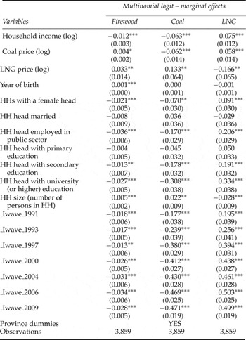
Ordered probit models assume the ordering of different fuels in terms of efficiency and convenience to use. As discussed in the empirical strategy section (see footnote 3), it can be argued that the households’ real ranking of the fuels may not be obvious and hence the multinomial logit model may be used alternatively. Nonetheless, the generalized ordered probit/logit model is preferable in cases where ordering is not ‘a priori obvious’ (Anderson, Reference Anderson1984) and the multinomial logit model can result in inefficient estimates if the ordering is inherent in the household fuel preference (Boes and Winkelmann, Reference Boes and Winkelmann2010). Therefore, we stick to the generalized ordered models (which are also better justified with the previous literature) in this paper. Yet, for comparison purposes, we also provide the marginal effects from the multinomial logit model in the appendix (table A1).Footnote 13 It can be seen from table A1 that the multinomial logit model generally supports our previous conclusions on the positive effects of raising households’ income, increasing coal price, empowering women, and higher education in helping the transition to clean energy. Meanwhile, the results from the multinomial model also suggest the importance of reducing LNG price (e.g., subsidizing LNG) in encouraging the usage of clean energy, which, however, is not well supported by the (RE and CORE) generalized ordered models above.
6. Conclusion and policy implications
Households' transition to modern energy sources can reduce the health and environmental impacts caused by the usage of traditional energy. Understanding the determinants of household fuel choice can provide policy implications for encouraging the adoption of cleaner and more efficient fuels in households. As the largest developing country in the world, China's evidence on this issue is of great interest. In contrast to previous studies on China, most of which are based on aggregate statistics or cross-sectional data from household surveys in a certain province or county, this paper employed the panel data from a nationwide survey (CHNS) to study the determinants of household fuel choice in urban China. Ordered probit models were employed in this study to take into account the potential ordering of different fuels in terms of efficiency or convenience to use, as in Farsi et al. (Reference Farsi, Filippini and Pachauri2007). Moreover, as mentioned above, we also made extensions to the applications of ordered discrete choice models to household fuel choice in terms of relaxing the parallel regression assumption and controlling the potential correlation between the explanatory variables and unobserved heterogeneity.
Our results indicate the heterogeneous effects of the explanatory variables across the distribution of different cooking fuels, which supports the use of the generalized ordered probit model. Also, the RE with Mundlak transformation approach generates results that are significantly different from those that are based on the standard random effects methods.
Furthermore, the results indicate that higher income leads to a lower probability of choosing low-ranked cooking fuel sources. Meanwhile, the results also show that, in addition to income, sociodemographic factors such as gender and education of the household heads are also important in determining the choices of primary cooking fuels in urban Chinese households. Thus, consistent with other recent studies (Masera et al., Reference Masera, Saatkamp and Kammen2000; Heltberg, Reference Heltberg2005; Farsi et al., Reference Farsi, Filippini and Pachauri2007), our results suggest that household fuel choice is not determined merely by a household's economic condition.
Coal price was also found to be important in household choices of primary cooking energy. An increase in the coal price is associated with a statistically significant decrease in the probability of choosing coal but a significant increase in the probability of choosing LNG or firewood as the primary cooking fuel. However, the effect of LNG price is found to be insignificant. From a policy point of view, these results indicate that interventions that reduce the price advantage of dirty fuels (e.g., taxing coal) may encourage households to use cleaner energy as their primary cooking fuel.
The tendency of households with female heads to be more likely to choose LNG as the primary cooking fuel and to reduce the usage of firewood implies that greater empowerment of women in the household can be helpful in increasing the usage of clean energy in urban China. In addition, the results that more education for household heads increases the probability of choosing LNG suggest that promotion of higher levels of education can be an effective way to encourage households to choose clean energy as the primary cooking fuel.
The estimated results of the year dummies indicates that more and more people are shifting over time from firewood and coal to LNG. The shift to LNG may also be associated with increased access to LNG over time, such as an increase in pipeline networks in urban China. In addition, the reduction in the usage of firewood in urban China over time may also be related to the introduction of more restrictive forest policies such as the NFCP.
However, this paper is not without limitations. For example, due to lack of information on the proportion of each fuel for the households who use multiple fuels, this study focused on the choice of primary cooking fuels and did not analyze multiple fuel use. Therefore, a direction for future research can be more comprehensive modeling of households' decision making on cooking fuels with consideration of all the fuels that a household can use. This will require richer data on households’ cooking fuel choices.
Appendix
Table A1. Marginal effect from the multinomial logit model