


Impact Statement
This paper discusses domain adaptation with transfer learning to transfer field-level pasture growing knowledge between locations with diverse climates for nitrogen response rate prediction in the context of agricultural digital twins.
1. Introduction
Decision support systems are widely used in agriculture to convert data to practical knowledge (Rinaldi and He, Reference Rinaldi, He and Sparks2014; Zhai et al., Reference Zhai, Martínez, Beltran and Martínez2020). A paradigm of decision support systems that has recently found its way to agriculture is that of digital twins (Pylianidis et al., Reference Pylianidis, Osinga and Athanasiadis2021). Digital twins are expected to merge the physical and virtual worlds by providing a holistic view of physical systems, through data integration, continuous monitoring, and adaptation to local conditions. They have started gaining traction with data architectures and applications for greenhouses (Howard et al., Reference Howard, Ma, Aaslyng and Jørgensen2020; Ariesen-Verschuur et al., Reference Ariesen-Verschuur, Verdouw and Tekinerdogan2022), conceptual frameworks for designing and developing them (Verdouw et al., Reference Verdouw, Tekinerdogan, Beulens and Wolfert2021), and case studies in aquaponics (Ghandar et al., Reference Ghandar, Ahmed, Zulfiqar, Hua, Hanai and Theodoropoulos2021).
A factor differentiating digital twins from existing systems is their ability to adapt to local conditions (Blair, Reference Blair2021). Following the digital twin paradigm, in contrast to generic models that apply global rules across all systems, we can create a blueprint that contains a high-level view of how a system works. This blueprint can then be instantiated as a digital twin in several systems, each with diverse local conditions, and further adjust to them, as more local data and feedback accumulate. In agriculture, adaptation to local conditions (or domain adaptation) is important because systems are affected by multiple local factors, and characterized by high uncertainty, also due to nature’s variability. Decisions have to account for the variability in weather conditions, soil types, and agricultural management (i.e. fertilization, irrigation, crop protection actions). Examples of failure to adapt include wrong estimations of yield (Parkes et al., Reference Parkes, Higginbottom, Hufkens, Ceballos, Kramer and Foster2019), failure to detect plant drought stress (Schmitter et al., Reference Schmitter, Steinrücken, Römer, Ballvora, Léon, Rascher and Plümer2017), and expensive equipment that does not work the way it is supposed to be (Gogoll et al., Reference Gogoll, Lottes, Weyler, Petrinic and Stachniss2020).
A challenge to apply domain adaptation techniques in agricultural digital twins lies with data-related issues. Process-based and machine learning (ML) models comprising the digital twins have difficulties operating with missing data or available data that do not conform with model requirements. ML models usually require large amounts of data to be trained, along with labels that are not readily available in agriculture. Also, it is beneficial for them to have data that cover large variability of the original domain, but usually the majority of the agricultural field observations are concentrated in a few locations with similar weather and the same agricultural practices. On the other hand, process-based models require their inputs to be complete. However, agricultural data are often sparse and noisy. Also, process-based models are typically numerical models that make predictions in small time intervals (from minutes to days). This can also be a problem as the prediction horizon is also short, or when those inputs are from future states of variables (e.g., weather and biophysical factors) and require additional tools to estimate them.
A workaround to data-related challenges is to use surrogate models, often also called metamodels. Metamodels mimic the behavior of other (typically more complex) models (Blanning, Reference Blanning1975). ML metamodels combine the advantages of ML models (learning patterns from data, operating with noisy data) and process-based models (operating based on first principles). A way to develop ML metamodels is to apply ML algorithms to the output of process-based model simulations. In this way, the ML algorithms can use a large corpus of synthetic data and, more importantly, extract the embedded domain knowledge contained in them. This technique has been proven to work well for instilling domain knowledge of water lake temperature to models (Karpatne et al., Reference Karpatne, Watkins, Read and Kumar2017) and working with data of different resolutions and absence of future weather values in nitrogen response rate (NRR) prediction (Pylianidis et al., Reference Pylianidis, Snow, Overweg, Osinga, Kean and Athanasiadis2022). However, the effectiveness of metamodels has not been investigated in conjunction with domain adaptation techniques in the context of agricultural digital twins.
Domain adaptation can be achieved with techniques like data assimilation and transfer learning. Data assimilation refers to the practice of calibrating a numerical model based on observations. This technique has been applied for grassland management digital twins (Purcell et al., Reference Purcell, Klipic and Neubauer2022), and digital twins for adaption to climate change (Bauer et al., Reference Bauer, Stevens and Hazeleger2021). Transfer learning refers to the utilization of knowledge obtained by training for a task, to solve a different but similar task. To the best of our knowledge, domain adaptation through transfer learning has not been thoroughly discussed in the context of digital twins for agriculture. An application we found was for plant disease identification, where the authors used a pretrained version of ImageNet and then continued training on a dataset containing images of diseased plants (Angin et al., Reference Angin, Anisi, Göksel, Gürsoy and Büyükgülcü2020). However, in other sectors, we find that transfer learning has been considered in several cases for digital twins (Xu et al., Reference Xu, Sun, Liu and Zheng2019; Voogd et al., Reference Voogd, Allamaa, Alonso-Mora and Son2022; Zhou et al., Reference Zhou, Sbarufatti, Giglio and Dong2022). Consequently, the applicability of transfer learning as a domain adaptation practice has not been extensively examined for agricultural digital twins.
In this work, we explore the potential of transfer learning to be used for domain adaptation in digital twins. To this end, we use a case study of digital twins predicting pasture NRRFootnote 1 at farm level. We use a synthetic dataset of grass pasture simulations and develop ML metamodels with transfer learning to investigate their adaption to new conditions. Our main question is:
-
• Q: How well can we transfer field-level knowledge from one location to another using transfer learning?
To answer this question, we examine it from different angles and form the following subquestions:
-
• Q1: How domain adaptation with transfer learning is affected by including more variability in agricultural management practices?
-
• Q2: How domain adaptation with transfer learning is affected by including more variability in weather data?
-
• Q3: How well does domain adaptation with transfer learning perform when applied to locations with different climate from the original one?
2. Methodology
2.1. Overview
To assess how well we can transfer field-level knowledge from one farm to another, we performed a case study of grass pasture NRR prediction in different locations across New Zealand. We have a dataset of pasture growth simulations based on historical weather data from sites with different climates (Figure 1), soil types, and fertilization treatments. Based on these data, we pretrained ML metamodels in an origin location and fine-tuned them in a target location to predict NRR and see how tuning affects model performance in both pretraining and fine-tuning test sets.

Figure 1. The sites contained in our dataset. With the brown color is the site in the origin climate (Marton, climate 1), and with the blue the sites in the target climates (Kokatahi and Lincoln, climates 2 and 3, respectively).
To obtain more dependable results, we pretrained in an origin climate and fine-tuned in two target climates that differ from each other. Also, we experimented with the amount of weather data included in the models as well as the number of soil types and fertilization levels. We created different setups and examined their results across several years, and for multiple runs using different seeds.
2.2. Data generation
The simulations comprising our dataset were generated with APSIM (Holzworth et al., Reference Holzworth, Huth, deVoil, Zurcher, Herrmann, McLean, Chenu, van Oosterom, Snow, Murphy, Moore, Brown, Whish, Verrall, Fainges, Bell, Peake, Poulton, Hochman, Thorburn, Gaydon, Dalgliesh, Rodriguez, Cox, Chapman, Doherty, Teixeira, Sharp, Cichota, Vogeler, Li, Wang, Hammer, Robertson, Dimes, Whitbread, Hunt, van Rees, McClelland, Carberry, Hargreaves, MacLeod, McDonald, Harsdorf, Wedgwood and Keating2014) using the AgPasture module (Li et al., Reference Li, Snow and Holzworth2011). This module has been proven to be an accurate estimator of pasture growth in New Zealand (Cichota et al., Reference Cichota, Snow and Vogeler2013, Reference Cichota, Vogeler, Werner, Wigley and Paton2018). The simulation parameters covered conditions that are known to affect pasture growth. The full factorial (Antony, Reference Antony and Antony2014) of those parameters was created and given as input to APSIM. The range of the parameters is shown in Table 1.
Table 1. The full factorial of the presented parameters was used to generate simulations with APSIM

2.3. Case study
In our experiments, we considered only the simulations where no irrigation was applied because this scenario is closer to the actual pasture growing conditions in New Zealand. Additionally, we only considered the autumn (March, April, and May) and spring (September, October, and November) months because these are the months in which agricultural practitioners are most interested in deciding how much fertilizer to apply.
To derive the NRR from the growth simulations, we calculated the additional amount of pasture dry matter harvested in the 2 months after fertilizer application per kg of nitrogen fertilizer applied.
Regarding the prediction scenario, we assumed to have weather and biophysical data only 4 weeks prior to the prediction date since pasture is supposed to not have memory beyond that point. Also, from the prediction date until the harvest date (2 months later), we assumed that no data were available.
2.4. Experimental setup
Throughout the setup, we create two types of models. The first type is trained on the data of the original location, and we call it “origin model.” The second type is fine-tuned with the data of the target location, by using the origin model as a basis, and we call it “target model.” We train different models using various setups which help us answer the sub-questions q1–q3. To answer q1, we considered two setups where variability comes from the number of agricultural management conditions included in the pretraining datasets:
-
• one type of soil and two types of fertilization treatments;
-
• three types of soil and five types of fertilization treatments.
To answer q2, we considered two setups where the digital twin blueprint contains training data from:
-
• 10 years of historical weather;
-
• 20 years of historical weather.
Consequently, for q1 and q2, there are four setups namely:
-
• low weather and agromanagement variabilities (s1);
-
• high weather variability, low agromanagement variability (s2);
-
• low weather variability, high agromanagement variability (s3);
-
• high weather and agromanagement variabilities (s4)
containing varying amounts of training data based on soil type, fertilization treatment, and the number of historical weather years. The details for each setup can be seen in (Figure A3). To answer q3, we considered three locations from our dataset with diverse climates. The origin location (location 1) where pretraining takes place, and two target locations. The target locations were selected based on the climate similarity index CCAFS (Ramirez-Villegas et al., Reference Ramirez-Villegas, Lau, Kohler, Jarvis, Arnell, Osborne and Hooker2011) to be dissimilar with the origin location to varying degrees (see Figure A1). Also, weather factors that are known to affect pasture growth were considered, namely precipitation and temperature. Location 2 is characterized by more frequent rainfall and lower temperatures than the origin location 1, and location 3 is characterized by less frequent rainfall and a wider range of temperatures than location 1. The respective plots can be seen in Figure A2.
Finally, we took measures to make the results more dependable. To alleviate the effect of imbalanced sets due to anomalous weather, we examined how transfer learning works across several years by sliding the corresponding training/validation/test sets across 5 years. Also, to see how robust the models were, we trained each one of them five times with different seeds in each setup and sliding year.
2.5. Data processing
The APSIM synthetic dataset was further processed to form a regression problem whose inputs were weather and biophysical variables as well as management practices. Initially, the NRR was calculated at 2 months after fertilization. Then, data were filtered to contain only simulations for the nonirrigated case. After that, only daily weather data in a window of 4 weeks prior to the prediction date were retained. Weather data between the prediction and target dates were also discarded because such data would be unavailable under operational conditions. Next, simulations with NRR less than 2 were removed as they were attributed to rare extreme weather phenomena that were not relevant to model for this study. From the remaining data, only the daily weather variables regarding precipitation, solar radiation, and minimum and maximum temperatures were preserved. From the biophysical outputs of APSIM only above ground pasture mass, herbage nitrogen concentration in dry matter, net increase in herbage above-ground dry matter, potential growth if there was no water and no nitrogen limitation soil, and temperature at 50 cm were preserved because they were considered likely drivers of yield (and known prior to the prediction date) based on expert knowledge. Additionally, from the simulation parameters, only soil fertility, soil water capacity, fertilizer amount, and fertilization month were retained to be put to the models as inputs. The data were then split into training/validation/test sets according to the experimental setup. Z-score normalization followed, with each test set being standardized with the scaler of the corresponding training set. The fertilization month column was transformed into a sine/cosine representation.
2.6. Neural network architecture
The selected architecture was a dual-head autoencoder, which proved to be accurate for NRR prediction tasks in another study (Pylianidis et al., Reference Pylianidis, Snow, Overweg, Osinga, Kean and Athanasiadis2022). The architecture consisted of an autoencoder with LSTM layers whose purpose is to learn to condense the input weather and biophysical time series, and a regression head with linear layers whose task is to predict the NRR (Figure 2). The combined loss is derived by summing the reconstruction loss and the NRR prediction loss.

Figure 2. The autoencoder architecture used to pretrain and fine-tune the models. The numbers on the top and bottom of the architecture indicate the number of features in the input/output of each component. The inputs to the encoder were nine time-series variables. The compressed representation of those time-series (output of LSTM 2) along with five scalars were concatenated and directed to a multi-layer perceptron.
The hyperparameters of the origin model were selected based on a preliminary study and were the same across all setups and years. For the target model, hyperparameter tuning was performed with gridsearch for each setup, year, and seed. The hyperparameters of the origin models and the search space for the target models can be seen in Tables A1 and A2.
For the part of tuning the network in different climates, no layer was frozen.
2.7. Evaluation
Pretrained and target models were evaluated on the test set of the origin location as well as the target location. This was done to examine how well they absorbed new information and how fast they were forgetting old information. The difference in performance between the origin and target models was measured with $ {R}^2 $
.
$ {R}^2 $
. $ {R}^2 $
was reported as an average across the five seeds, for each setup, and each year. Also, the standard deviations of
$ {R}^2 $
was reported as an average across the five seeds, for each setup, and each year. Also, the standard deviations of $ {R}^2 $
between the seeds were examined to see how stable the performance is across the runs.
$ {R}^2 $
between the seeds were examined to see how stable the performance is across the runs.
3. Results
For both target locations, we observe that fine-tuning increased the average $ {R}^2 $
across the runs on the target location test set for most setups. For s1 and s2, this behavior was consistent in both location 2 (Figure 3) and location 3 (Figure 4). For s3, tuning offered marginal improvements in both locations. In the case of s4, the results varied between the locations, as in location 2, there was no improvement and even degradation in years 2004–2005 (Figure 3d), and in location 3 minor improvements (Figure 4d). The standard deviations of the target models on the target location test sets were within the [0.01, 0.08] range (Figures A4 and A5).
$ {R}^2 $
across the runs on the target location test set for most setups. For s1 and s2, this behavior was consistent in both location 2 (Figure 3) and location 3 (Figure 4). For s3, tuning offered marginal improvements in both locations. In the case of s4, the results varied between the locations, as in location 2, there was no improvement and even degradation in years 2004–2005 (Figure 3d), and in location 3 minor improvements (Figure 4d). The standard deviations of the target models on the target location test sets were within the [0.01, 0.08] range (Figures A4 and A5).
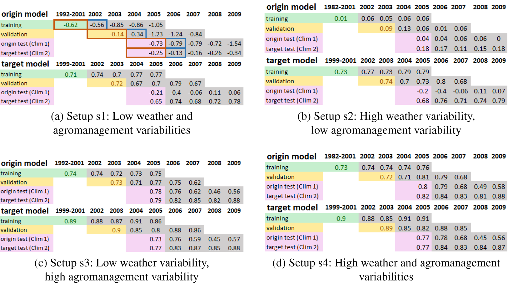
Figure 3. $ {R}^2 $
for the setups of the origin models (climate 1), and target models in climate 2. The results are presented as averages across the five seeds for each setup and year. On Figure 3a, the brown and blue colors indicate which training, validation and test set correspond to each experiment due to the sliding years. Same colors represent sets of the same experiment. For example, with the brown color the training set of the origin model included years 1992–2001, validation set 2002–2003, and both test sets years 2004–2005. On the experiment with the blue color the training set included years 1993–2002, validation 2003–2004, and both test sets 2005–2006. The leftmost cell of the results is colored (green, yellow, pink) as the corresponding set is colored, and has a width equal to the amount of training years included in it. For the other four sliding years, only the last year of each set is shown with gray color.
$ {R}^2 $
for the setups of the origin models (climate 1), and target models in climate 2. The results are presented as averages across the five seeds for each setup and year. On Figure 3a, the brown and blue colors indicate which training, validation and test set correspond to each experiment due to the sliding years. Same colors represent sets of the same experiment. For example, with the brown color the training set of the origin model included years 1992–2001, validation set 2002–2003, and both test sets years 2004–2005. On the experiment with the blue color the training set included years 1993–2002, validation 2003–2004, and both test sets 2005–2006. The leftmost cell of the results is colored (green, yellow, pink) as the corresponding set is colored, and has a width equal to the amount of training years included in it. For the other four sliding years, only the last year of each set is shown with gray color.

Figure 4. Average $ {R}^2 $
for the various setups of the origin models (climate 1), and target models in climate 3. The figures should be read following the pattern of Figure 3a.
$ {R}^2 $
for the various setups of the origin models (climate 1), and target models in climate 3. The figures should be read following the pattern of Figure 3a.
Tuning also increased the average $ {R}^2 $
on the origin location test set for s1 (Figure 3a,b) and s2 (Figure 4a,b). However, on s3 and s4, the performance remained stable or deteriorated depending on the year. The standard deviations of the target models on the origin location test sets were within the [0.01, 0.3] range. The standard deviation of the target models on the pretraining test sets for s1 and s2 were within the range [0.03, 0.32], and for s3 and s4 [0.02, 0.19].
$ {R}^2 $
on the origin location test set for s1 (Figure 3a,b) and s2 (Figure 4a,b). However, on s3 and s4, the performance remained stable or deteriorated depending on the year. The standard deviations of the target models on the origin location test sets were within the [0.01, 0.3] range. The standard deviation of the target models on the pretraining test sets for s1 and s2 were within the range [0.03, 0.32], and for s3 and s4 [0.02, 0.19].
Another observation is that the $ {R}^2 $
of the origin model on s1 was negative in both locations for all years (Figures 3a, 4a). The corresponding standard deviations were also high as shown in Figures A4a, A5a.
$ {R}^2 $
of the origin model on s1 was negative in both locations for all years (Figures 3a, 4a). The corresponding standard deviations were also high as shown in Figures A4a, A5a.
A remark is also the high volatility of $ {R}^2 $
depending on the year, of both origin and target models in the origin and target locations test sets. Performance becomes more stable as more weather and agromanagement variability are added (e.g., s1–s2, s1–s3) but there were years like 2004–2005 in location 2, 2008–2009 on location 3 where
$ {R}^2 $
depending on the year, of both origin and target models in the origin and target locations test sets. Performance becomes more stable as more weather and agromanagement variability are added (e.g., s1–s2, s1–s3) but there were years like 2004–2005 in location 2, 2008–2009 on location 3 where $ {R}^2 $
dropped substantially. The standard deviations (Figures A4 and A5) also became lower across the years as more agromanagement variability was added.
$ {R}^2 $
dropped substantially. The standard deviations (Figures A4 and A5) also became lower across the years as more agromanagement variability was added.
One more finding is that adding more weather variability while keeping the agromanagement practices unchanged had a negligible (positive) effect on the performance of the target models. This pattern can be observed for both locations when transitioning from s1 to s2 (e.g., Figure 3a,b), and from s3 to s4 throughout the years (e.g., Figure 3c,d). Also, in those scenarios, the standard deviations of the target models on the pretraining test sets did not decrease when extra weather variability was added. On the other hand, increasing the management practices while keeping the same weather variability seemed to increase the $ {R}^2 $
of both models in both test sets. This can be seen when transitioning from s1 to s3 (e.g., Figure 4a–c), and from s2 to s4 (e.g., Figure 4b–d).
$ {R}^2 $
of both models in both test sets. This can be seen when transitioning from s1 to s3 (e.g., Figure 4a–c), and from s2 to s4 (e.g., Figure 4b–d).
4. Discussion
Starting with some general remarks about model performance, for transfer learning tasks there is usually a model that works well which then undergoes further training. Here, the first impression is that the performance of the origin model on s1 and s2 is inadequate. This is potentially due to the selected architecture and the way training was performed. In those setups, the samples were too few (see Figure A3), and the architecture had a lot of weights. As a result, the network may not have been able to extract meaningful features in those cases. Also, the performance increase on the pretraining test set after tuning may indicate that extra information is included in the tuning training data, but it could also mean that the worse performance was due to training for too few epochs.
Another remark is that the target models achieve considerably higher $ {R}^2 $
on location 2 than on location 3. This behavior could be attributed to the weather conditions of each location. Location 2 is characterized by more precipitation, reducing in this way the uncertainty of having less water during the period of 60 days that for which we assume that no weather data are available from the prediction to the target date. As a result, the NRR values concentrate on a narrower range, and models have an easier task explaining variance.
$ {R}^2 $
on location 2 than on location 3. This behavior could be attributed to the weather conditions of each location. Location 2 is characterized by more precipitation, reducing in this way the uncertainty of having less water during the period of 60 days that for which we assume that no weather data are available from the prediction to the target date. As a result, the NRR values concentrate on a narrower range, and models have an easier task explaining variance.
Regarding fine-tuning, it seems to make the models able to generalize better in the target locations than the models which have not seen this extra information before. Especially for setups s1 and s2, the results indicate that transfer learning adds value when the available soil, and fertilization management data are limited in quantity. This statement is supported by the consistency of the results which come from several years, and two diverse locations, suggesting that this behavior is not year or location dependent. For the same setups, the decrease in the standard deviation after fine-tuning strengthens the claim that the improved performance is not a coincidence.
On the contrary, when there is sufficient variability in the soil and fertilization management practices, the role of fine-tuning becomes ambiguous. It may seem that transfer learning increases the generalization capacity of the models for most of s3 and s4 cases, even though improvements are marginal. However, these improvements are so small that they get counteracted by the standard deviation of the successive runs. Also, depending on the year (e.g., 2004–2005 for location 2) fine-tuning may be harmful as it decreases $ {R}^2 $
further than the standard deviation of the five runs. Performing more runs with different seeds or testing in different years could potentially yield different results than those observed. Consequently, we cannot assess the merits of fine-tuning in those cases.
$ {R}^2 $
further than the standard deviation of the five runs. Performing more runs with different seeds or testing in different years could potentially yield different results than those observed. Consequently, we cannot assess the merits of fine-tuning in those cases.
Moving on to the effect of adding more weather variability in the origin models, we saw that the differences in performance were small. This pattern was observed for both target locations, and the reasons behind its appearance may vary. We could presume that adding weather variability does not help the models enough to extract information relevant to NRR prediction. This could be the case if in those extra years the weather was very different from the weather of the target locations. Another case would be that since we have a gap of 60 days between the prediction and target dates, and assuming the absence of extreme phenomena, the weather is more loosely connected to the NRR prediction than other factors like soil type and fertilization practices.
A more apparent reason for the effect of adding more weather variability is that we potentially observe the effect of increasingly higher sample sizes. In Figure A3, we see the number of samples in each setup. Adding more weather data (s1–s2, or s3–s4) doubles the samples included in the pretraining data. However, with the current experimental setup, adding soil types and fertilization treatments (s1–s3, or s2–s4) increases the number of samples by a much higher degree. Therefore, adding more weather variability to the pretraining sets has little (but positive) effect on the model test sets, which seems small compared to adding more soil types and fertilization treatments because with the latter we have many more samples. The increase of $ {R}^2 $
of the target models on the pretraining test sets seems to support this argument. Adding more weather data to a model from a target location could help explain the variability in that location. However, here we see that it also helps to explain variance in the original location, prompting that this increase is not due to the so different conditions supposedly existing on the new data but just an increased sample size. For this reason, this phenomenon is more evidently expressed at s1 and s2 where sample sizes are lower.
$ {R}^2 $
of the target models on the pretraining test sets seems to support this argument. Adding more weather data to a model from a target location could help explain the variability in that location. However, here we see that it also helps to explain variance in the original location, prompting that this increase is not due to the so different conditions supposedly existing on the new data but just an increased sample size. For this reason, this phenomenon is more evidently expressed at s1 and s2 where sample sizes are lower.
5. Limitations
There are cases where it is unclear if the improvement in $ {R}^2 $
on the tuning location test set comes from adding samples with information about local conditions or from just the continuation of training with extra samples. To be able to better deduct those cases the set sizes should be equal between the different setups s1–s4. The challenge there would be to create representative sets for all setups, sliding years, and target locations.
$ {R}^2 $
on the tuning location test set comes from adding samples with information about local conditions or from just the continuation of training with extra samples. To be able to better deduct those cases the set sizes should be equal between the different setups s1–s4. The challenge there would be to create representative sets for all setups, sliding years, and target locations.
Another limitation is that we used the same neural network architecture for all the setups. This architecture has many weights that need to be calibrated and in setups with fewer samples, it may not be appropriate to use. A simpler architecture might have given different results.
With the provided experimental setup, we created two types of models, the “pretrained” (origin) and “fine-tuned” (target). The origin models contained an increasing number of samples from the origin location based on the setup, and the fine-tuned a fixed number of samples from the target location. However, we did not include in the study the results of models trained only on the data from the target location. Preliminary tests with the chosen architecture showed that such models had negative $ {R}^2 $
in all setups and high standard deviations, so they were omitted. A more thorough investigation would include such models with simpler architectures, or different algorithms with features aggregated on a weekly/biweekly basis to decrease the number of parameters that have to be calibrated.
$ {R}^2 $
in all setups and high standard deviations, so they were omitted. A more thorough investigation would include such models with simpler architectures, or different algorithms with features aggregated on a weekly/biweekly basis to decrease the number of parameters that have to be calibrated.
In regards to the data splits, in a more practical application the test set years would be closer to the training set years. With the current setup, the training and test sets are 2 or 3 years apart. With such gaps, the weather may change substantially leading to nonrepresentative sets. An alternative setup would be to have these years closer and maybe remove the validation set and perform a k-fold cross validation for hyperparameter tuning instead.
6. Conclusion
In this work, we examined the application of transfer learning as a way to make field-level pasture digital twins adapt to local conditions. We employed a case study of pasture NRR prediction, and investigated factors that affect the efficiency of the adaptation procedure. Different setups had varying outcomes but generally transfer learning seems to provide a promising way for digital twins to learn the idiosyncrasies of different locations.
Revisiting q1, based on our experiments variability in soil type and fertilization treatment seemed to help the models explain a large fraction of variance in the target locations. Therefore, for field-deployed applications, practitioners could try to gather as much data as possible with this kind of variability or generate them. On the other hand, for q2 we found that the addition of extra weather variability had a small impact on model performance. Thus, adding more variability in soil and agricultural management practices should be of higher priority. In both cases, more work is needed to verify the degree to which large sample sizes start to affect the results. Regarding q3, transfer learning appears to work for diverse climates with performance differences depending on the prevailing local conditions. Again, more work is needed to test its efficiency in climates that are even more diverse and characterized by more extreme phenomena.
Finally, to answer our main question, the above are evidence that we can transfer field-level knowledge to a degree that models can explain an adequate portion of variance in the target locations. In this respect, transfer learning has the potential for making digital twins adapt to different conditions by working in different climates, and with different types of variability. Practitioners could create blueprints of digital twins with origin models and then adapt to different locations by instantiating them there preferably with samples that contain varied soil types and fertilization treatments.
Acknowledgments
The authors are extremely grateful to Dr. Val Snow (AgResearch, NZ) for generating the synthetic dataset using APSIM and her contributions in designing the case study application (Pylianidis et al., Reference Pylianidis, Snow, Overweg, Osinga, Kean and Athanasiadis2022). The authors would like to thank Dr. Dilli Paudel (Wageningen University & Research) for the constructive discussions during the validation phase of the experiments.
Author contribution
Conceptualization: C.P., I.A.; Data curation: C.P.; Data visualization: C.P., M.K.; Methodology: C.P., I.A.; Validation: C.P., I.A., M.K.; Writing—original draft: C.P.; Writing—review and editing: I.A., M.K. All authors approved the final submitted draft.
Competing interest
The authors declare none.
Data availability statement
Replication code can be found in https://github.com/BigDataWUR/Domain-adaptation-for-pasture-digital-twins.
Ethics statement
The research meets all ethical guidelines, including adherence to the legal requirements of the study country.
Funding statement
C.P. has been partially supported by the European Union Horizon 2020 Research and Innovation program (Grant No. 810775, Dragon). M.K. has been partially supported by the European Union Horizon Europe Research and Innovation program (Grant No. 101070496, Smart Droplets).
A. Appendix
A.1. Climate similarity

Figure A1. CCAFS similarity index across New Zealand. The weather parameters for the similarity were precipitation and average temperature. Location 1 (Marton) is colored in brown, and locations 2 (Kokatahi) and 3 (Lincoln) in blue. The darker the color on the map, the more similar the climate is to location 1. Location 2 had index value 0.354, and location 3 0.523.

Figure A2. Weather parameters known to affect pasture growth for the climates included in this study. The parameters are presented across the months and are aggregated over the years.
A.2. Experimental setup simulation parameters and amount of samples

Figure A3. Number of parameters and total samples used in each training/validation/test set of each setup.
A.3. Model hyperparameters
Table A1. The fixed hyperparameters of the origin models
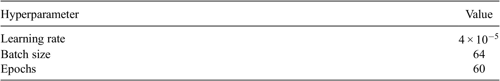
Table A2. The search space for the hyperparameters of the target models

A.4. Results—standard deviations

Figure A4. Standard deviations of the various setups for origin models (climate 1), and target models in climate 2.

Figure A5. Standard deviations of the various setups for the origin models climate 1, and target models in climate 2.


 Open access