


1 Introduction
In the study of the dynamics of complex analytic functions one of the most well-studied and important families of functions is the exponential family $E_{\kappa }:z\mapsto \kappa e^z$
,
$E_{\kappa }:z\mapsto \kappa e^z$
, $\kappa \in \mathbb {C}-\{0\}$
. Perhaps the most fundamental fact about this family concerns its Julia set. The Julia set
$\kappa \in \mathbb {C}-\{0\}$
. Perhaps the most fundamental fact about this family concerns its Julia set. The Julia set $\mathcal {J}(f)$
of an entire function f is the set of all points in the complex plane where the family of iterates
$\mathcal {J}(f)$
of an entire function f is the set of all points in the complex plane where the family of iterates $f^n$
of f is not normal. For
$f^n$
of f is not normal. For $0<\kappa \leq 1/e$
, as was proved first by Devaney and Krych in [Reference Devaney and Krych13], the Julia set
$0<\kappa \leq 1/e$
, as was proved first by Devaney and Krych in [Reference Devaney and Krych13], the Julia set ${\mathcal {J}}(E_{\kappa })$
is a so-called Cantor bouquet which consists of uncountably many disjoint curves each of which has a finite endpoint and goes off to infinity. On the other hand, when
${\mathcal {J}}(E_{\kappa })$
is a so-called Cantor bouquet which consists of uncountably many disjoint curves each of which has a finite endpoint and goes off to infinity. On the other hand, when $\kappa>1/e$
, Misiurewicz in [Reference Misiurewicz23] proved that the Julia set
$\kappa>1/e$
, Misiurewicz in [Reference Misiurewicz23] proved that the Julia set ${\mathcal {J}}(E_{\lambda })$
equals the entire complex plane
${\mathcal {J}}(E_{\lambda })$
equals the entire complex plane $\mathbb {C}$
(actually Misiurewicz only proved this for
$\mathbb {C}$
(actually Misiurewicz only proved this for $\kappa =1$
but his proof can easily be adapted to cover the other cases as well; see [Reference Devaney10]). For a different proof of the same fact, see [Reference Shen and Rempe-Gillen29]. For all these facts and much more we refer to Devaney’s survey [Reference Devaney, Broer, Hasselblatt and Takens11] on exponential dynamics.
$\kappa =1$
but his proof can easily be adapted to cover the other cases as well; see [Reference Devaney10]). For a different proof of the same fact, see [Reference Shen and Rempe-Gillen29]. For all these facts and much more we refer to Devaney’s survey [Reference Devaney, Broer, Hasselblatt and Takens11] on exponential dynamics.
In recent years there has been increasing interest in the study of dynamics of quasiregular functions. Quasiregular functions are a higher-dimensional generalization of holomorphic maps on the plane. We refer to [Reference Bergweiler2] for a survey on the dynamics of such functions. As Bergweiler and Nicks have shown in [Reference Bergweiler4, Reference Bergweiler and Nicks5], there is a sensible definition for the Julia set for such functions which has many of the properties of the classical Julia set.
Moreover, in this higher-dimensional setting, there is a whole family of maps that can be considered analogues of the exponential map, called the Zorich maps, which are quasiregular and were first constructed by Zorich in [Reference Zorich33]. Following [Reference Iwaniec and Martin18], we describe the construction of the Zorich maps in three dimensions. Note that the construction can be done in arbitrary dimensions but we will confine ourselves to three dimensions for simplicity. First consider an L bi-Lipschitz, sense-preserving map $\mathfrak {h}$
that maps the square
$\mathfrak {h}$
that maps the square
 $$ \begin{align*} Q:= \{(x_1,x_2)\in\mathbb{R}^2:|x_1|\leq 1,|x_2|\leq 1 \} \end{align*} $$
to the upper hemisphere
 $$ \begin{align*} \{(x_1,x_2,x_3)\in\mathbb{R}^3:x_1^2+x_2^2+x_3^2=1, x_3\geq 0\}. \end{align*} $$
Then define the map $Z:Q\times \mathbb {R}\to \mathbb {R}^3$
as
$Z:Q\times \mathbb {R}\to \mathbb {R}^3$
as
 $$ \begin{align*} Z(x_1,x_2,x_3)=e^{x_3}\mathfrak{h}(x_1,x_2). \end{align*} $$
This maps the square beam $Q\times \mathbb {R}$
to the upper half-space. By repeatedly reflecting now, across the sides of the square beam in the domain and the
$Q\times \mathbb {R}$
to the upper half-space. By repeatedly reflecting now, across the sides of the square beam in the domain and the $x_1x_2$
plane in the range, we obtain a map
$x_1x_2$
plane in the range, we obtain a map $Z:\mathbb {R}^3\to \mathbb {R}^3$
. Note that this map is doubly periodic, meaning that
$Z:\mathbb {R}^3\to \mathbb {R}^3$
. Note that this map is doubly periodic, meaning that $Z(x_1+4,x_2,x_3)=Z(x_1,x_2+4,x_3)=Z(x_1,x_2,x_3)$
. Moreover, the map is not locally injective everywhere. The lines
$Z(x_1+4,x_2,x_3)=Z(x_1,x_2+4,x_3)=Z(x_1,x_2,x_3)$
. Moreover, the map is not locally injective everywhere. The lines $x_1=2n+1, x_2=2m+1$
,
$x_1=2n+1, x_2=2m+1$
, $n,m\in \mathbb {Z}$
, belong to the branch set, namely the set
$n,m\in \mathbb {Z}$
, belong to the branch set, namely the set
 $$ \begin{align*} \mathcal{B}_{Z}:=\{x\in\mathbb{R}^3:Z \ \text{is not locally homeomorphic at}\ x\}. \end{align*} $$
Also it can be shown that the map is quasiregular and has an essential singularity at infinity, just like the exponential map on the plane. Although we will not need this, we say that such quasiregular maps are of transcendental type.
We can also introduce a parameter $\nu>0$
and consider the family
$\nu>0$
and consider the family $Z_{\nu }=\nu Z$
, where Z is a Zorich map. This family can be considered as an analogue of the exponential family in higher dimensions (at least in the case where
$Z_{\nu }=\nu Z$
, where Z is a Zorich map. This family can be considered as an analogue of the exponential family in higher dimensions (at least in the case where $\kappa>0$
). Hence, it would be very interesting to know whether or not this family has similar behaviour to the exponential in terms of dynamics. Indeed, Bergweiler in [Reference Bergweiler3] and Bergweiler and Nicks in [Reference Bergweiler and Nicks5, §7] have proved that for small values of
$\kappa>0$
). Hence, it would be very interesting to know whether or not this family has similar behaviour to the exponential in terms of dynamics. Indeed, Bergweiler in [Reference Bergweiler3] and Bergweiler and Nicks in [Reference Bergweiler and Nicks5, §7] have proved that for small values of $\nu $
this family has as its Julia set uncountably many, pairwise disjoint curves. For those curves, Bergweiler in [Reference Bergweiler3] proved a counterpart to Karpinska’s paradox (see [Reference Karpińska19, Reference Karpińska20]) for the exponential map, namely the fact that the endpoints of those curves have Hausdorff dimension three while the curves minus the endpoints have Hausdorff dimension one. Moreover, Comdühr in [Reference Comdühr6] proved that those curves are smooth, generalizing a result of Viana da Silva [Reference Viana da Silva31], and in [Reference Tsantaris30] we studied the topology of those curves. It is also worth mentioning here that Cantor bouquets have been proved to exist for other generalized exponential functions, not necessarily quasiregular (see [Reference Comdühr, Evdoridou and Sixsmith7]). Having said all that, it seems quite reasonable to expect that for large values of
$\nu $
this family has as its Julia set uncountably many, pairwise disjoint curves. For those curves, Bergweiler in [Reference Bergweiler3] proved a counterpart to Karpinska’s paradox (see [Reference Karpińska19, Reference Karpińska20]) for the exponential map, namely the fact that the endpoints of those curves have Hausdorff dimension three while the curves minus the endpoints have Hausdorff dimension one. Moreover, Comdühr in [Reference Comdühr6] proved that those curves are smooth, generalizing a result of Viana da Silva [Reference Viana da Silva31], and in [Reference Tsantaris30] we studied the topology of those curves. It is also worth mentioning here that Cantor bouquets have been proved to exist for other generalized exponential functions, not necessarily quasiregular (see [Reference Comdühr, Evdoridou and Sixsmith7]). Having said all that, it seems quite reasonable to expect that for large values of $\nu $
the Julia set of the Zorich family would be the whole of
$\nu $
the Julia set of the Zorich family would be the whole of $\mathbb {R}^3$
just like in the exponential family where the Julia set is the entire complex plane. One aim of this paper is to prove that if we make some reasonable modifications to the map
$\mathbb {R}^3$
just like in the exponential family where the Julia set is the entire complex plane. One aim of this paper is to prove that if we make some reasonable modifications to the map $\mathfrak {h}$
then this conjecture holds.
$\mathfrak {h}$
then this conjecture holds.
Let us now define the modified $\mathfrak {h}$
and state our main theorem. The first thing that we require is that our map
$\mathfrak {h}$
and state our main theorem. The first thing that we require is that our map $\mathfrak {h}(x_1,x_2)=(\mathfrak {h}_1(x_1,x_2),\mathfrak {h}_2(x_1,x_2),\mathfrak {h}_3(x_1,x_2))$
must satisfy
$\mathfrak {h}(x_1,x_2)=(\mathfrak {h}_1(x_1,x_2),\mathfrak {h}_2(x_1,x_2),\mathfrak {h}_3(x_1,x_2))$
must satisfy $\mathfrak {h}_1(x_1,x_1)=\mathfrak {h}_2(x_1,x_1)$
and
$\mathfrak {h}_1(x_1,x_1)=\mathfrak {h}_2(x_1,x_1)$
and $\mathfrak {h}_1(x_1,-x_1)=-\mathfrak {h}_2(x_1,-x_1)$
. In this way the planes
$\mathfrak {h}_1(x_1,-x_1)=-\mathfrak {h}_2(x_1,-x_1)$
. In this way the planes $x_1=x_2$
and
$x_1=x_2$
and $x_1=-x_2$
are invariant under the Zorich map we obtain. Note that this implies that
$x_1=-x_2$
are invariant under the Zorich map we obtain. Note that this implies that $\mathfrak {h}(0,0)=(0,0,1)$
. Second, we need to scale things by a factor
$\mathfrak {h}(0,0)=(0,0,1)$
. Second, we need to scale things by a factor $\lambda>1$
. To be more precise, we define the function
$\lambda>1$
. To be more precise, we define the function
 $$ \begin{align*} h(x_1,x_2)=\lambda \mathfrak{h}\bigg(\frac{1}{\lambda}(x_1,x_2)\bigg), \quad (x_1,x_2)\in\lambda Q. \end{align*} $$
We now define the Zorich maps we obtain by this h, which we denote by $\mathcal {Z}$
:
$\mathcal {Z}$
:
 $$ \begin{align} \mathcal{Z}_{\nu}(x_1,x_2,x_3)=\nu e^{x_3}h(x_1,x_2),\quad (x_1,x_2,x_3)\in \lambda Q\times \mathbb{R},\ \nu>0. \end{align} $$
Again we extend this map to $\mathbb {R}^3$
by reflecting across the sides of the square beam and the plane
$\mathbb {R}^3$
by reflecting across the sides of the square beam and the plane $x_3=0$
. Another important thing to note here is that during the process of extending our map
$x_3=0$
. Another important thing to note here is that during the process of extending our map $\mathcal {Z}_\nu $
from the initial square beam to the whole of
$\mathcal {Z}_\nu $
from the initial square beam to the whole of $\mathbb {R}^3$
we can also extend
$\mathbb {R}^3$
we can also extend $\mathfrak {h}$
to a Lipschitz map from
$\mathfrak {h}$
to a Lipschitz map from $\mathbb {R}^2$
to
$\mathbb {R}^2$
to $\mathbb {R}^3$
with the same Lipschitz constant L. We will always assume that this extension has been done, and when we talk about
$\mathbb {R}^3$
with the same Lipschitz constant L. We will always assume that this extension has been done, and when we talk about $\mathfrak {h}$
we will mean the extended one unless otherwise stated. Moreover, let us note here that this new Zorich map
$\mathfrak {h}$
we will mean the extended one unless otherwise stated. Moreover, let us note here that this new Zorich map $\mathcal {Z}$
is conjugate to
$\mathcal {Z}$
is conjugate to $x\mapsto Z(x_1,x_2,\lambda x_3)$
, where Z is the classic Zorich map without the scaling.
$x\mapsto Z(x_1,x_2,\lambda x_3)$
, where Z is the classic Zorich map without the scaling.
Remark 1 Here it is worth elaborating on that last sentence. Instead of studying the family $\mathcal {Z}_\nu $
, defined in (1.1), we could have studied the family
$\mathcal {Z}_\nu $
, defined in (1.1), we could have studied the family $\alpha \circ Z$
, where
$\alpha \circ Z$
, where $\alpha :\mathbb {R}^3\to \mathbb {R}^3$
is the linear map induced by the matrix
$\alpha :\mathbb {R}^3\to \mathbb {R}^3$
is the linear map induced by the matrix
 $$ \begin{align*}\begin{pmatrix} \nu& 0&0\\ 0& \nu &0\\ 0&0&\nu\lambda \end{pmatrix}\end{align*} $$
and Z is the Zorich map that leaves the planes $x_1=\pm x_2$
invariant and comes from using
$x_1=\pm x_2$
invariant and comes from using $\mathfrak {h}$
. It is easy to see that the map
$\mathfrak {h}$
. It is easy to see that the map $\alpha \circ Z$
is conjugate to
$\alpha \circ Z$
is conjugate to $\nu Z(x_1,x_2,\lambda x_3)$
and thus to
$\nu Z(x_1,x_2,\lambda x_3)$
and thus to $\mathcal {Z}_\nu $
. The advantage of this viewpoint is that the Zorich maps we consider here and the maps considered by Bergweiler in [Reference Bergweiler3] can all be seen as maps in the space
$\mathcal {Z}_\nu $
. The advantage of this viewpoint is that the Zorich maps we consider here and the maps considered by Bergweiler in [Reference Bergweiler3] can all be seen as maps in the space $\{\mathcal {A}\circ Z:\mathcal {A}\in \mathrm {GL}_3(\mathbb {R})\}$
, where
$\{\mathcal {A}\circ Z:\mathcal {A}\in \mathrm {GL}_3(\mathbb {R})\}$
, where $\mathrm {GL}_3(\mathbb {R})$
is the general linear group of degree
$\mathrm {GL}_3(\mathbb {R})$
is the general linear group of degree $3$
. Thus
$3$
. Thus $\mathrm {GL}_3(\mathbb {R})\setminus \{0\}$
becomes the parameter space for Zorich maps in analogy with
$\mathrm {GL}_3(\mathbb {R})\setminus \{0\}$
becomes the parameter space for Zorich maps in analogy with $\mathbb {C}\setminus \{0\}$
being the parameter space for the exponential map.
$\mathbb {C}\setminus \{0\}$
being the parameter space for the exponential map.
Due to conjugacy, all of the theorems we will prove here are also true for the family $\alpha \circ Z$
. We have chosen to use a different presentation of Zorich maps than the one described here since that way the definition seems more natural and the connection with the exponential family is more apparent.
$\alpha \circ Z$
. We have chosen to use a different presentation of Zorich maps than the one described here since that way the definition seems more natural and the connection with the exponential family is more apparent.
For the type of Zorich maps defined in (1.1) we will prove the following result.
Theorem 1 Let $\lambda>L^{5}$
. Then for all
$\lambda>L^{5}$
. Then for all $\nu> \sqrt {{2L}/{\lambda }}$
the Zorich map
$\nu> \sqrt {{2L}/{\lambda }}$
the Zorich map $\mathcal {Z}_{\nu }$
we obtain using this scale factor
$\mathcal {Z}_{\nu }$
we obtain using this scale factor $\lambda $
has as its Julia set the whole of
$\lambda $
has as its Julia set the whole of $\mathbb {R}^3$
.
$\mathbb {R}^3$
.
Remark 2 We will actually prove a slightly stronger result. Namely, that if the assumptions of the above theorem are satisfied and V is any open set of $\mathbb {R}^3$
then
$\mathbb {R}^3$
then $\bigcup _{n\geq 0}\mathcal {Z}_{\nu }^n(V)$
covers
$\bigcup _{n\geq 0}\mathcal {Z}_{\nu }^n(V)$
covers $\mathbb {R}^3\setminus \{0\}$
.
$\mathbb {R}^3\setminus \{0\}$
.
Theorem 1 implies that the behaviour of the iterates of the Zorich maps, for those particular choices of the parameters, are chaotic in the whole of $\mathbb {R}^3$
. The method we use in the proof of Theorem 1 also allows us to prove a theorem on the measurable dynamics of Zorich maps which can be seen as analogous to a theorem for exponential maps due to Ghys, Sullivan and Goldberg (see Theorem 7 in §8 for more details). Another fact usually associated with chaotic behaviour in a set is the density of periodic points on that set. In the complex plane it is well known, and was first proved by Baker in [Reference Baker1], that periodic points of an entire transcendental map (in fact even repelling periodic points) are dense in its Julia set. However, it still unknown whether or not the periodic points of a quasiregular map on
$\mathbb {R}^3$
. The method we use in the proof of Theorem 1 also allows us to prove a theorem on the measurable dynamics of Zorich maps which can be seen as analogous to a theorem for exponential maps due to Ghys, Sullivan and Goldberg (see Theorem 7 in §8 for more details). Another fact usually associated with chaotic behaviour in a set is the density of periodic points on that set. In the complex plane it is well known, and was first proved by Baker in [Reference Baker1], that periodic points of an entire transcendental map (in fact even repelling periodic points) are dense in its Julia set. However, it still unknown whether or not the periodic points of a quasiregular map on $\mathbb {R}^3$
are dense in its Julia set. We are able to prove that this is indeed the case for Zorich maps.
$\mathbb {R}^3$
are dense in its Julia set. We are able to prove that this is indeed the case for Zorich maps.
Theorem 2 Let $\nu $
and
$\nu $
and $\lambda $
be as in Theorem 1. The periodic points of
$\lambda $
be as in Theorem 1. The periodic points of $\mathcal {Z}_{\nu }$
are dense in
$\mathcal {Z}_{\nu }$
are dense in $\mathbb {R}^3$
.
$\mathbb {R}^3$
.
Another object of study in the exponential family, and in transcendental complex dynamics in general, which is intimately connected with the Julia set is the escaping set. It was first studied by Eremenko in [Reference Eremenko15], and if $f:\mathbb {C}\to \mathbb {C}$
is an entire function then it is defined as
$f:\mathbb {C}\to \mathbb {C}$
is an entire function then it is defined as
 $$ \begin{align*} I(f):=\{z\in \mathbb{C}:|f^n(z)|\to\infty \ \text{as}\ n\to\infty\}. \end{align*} $$
Eremenko proved that $I(f)\not =\emptyset $
and that
$I(f)\not =\emptyset $
and that $\partial I(f)=\mathcal {J}(f)$
.
$\partial I(f)=\mathcal {J}(f)$
.
Moreover, for the exponential family from [Reference Eremenko and Lyubich14] it is true that ${I(f)}\subset \mathcal {J}(f)$
and thus
${I(f)}\subset \mathcal {J}(f)$
and thus $I(f)$
is dense in the Julia set. When the Julia set is a Cantor bouquet, the escaping set consists of the disjoint curves that make up the Julia set together with some of their endpoints. In this case
$I(f)$
is dense in the Julia set. When the Julia set is a Cantor bouquet, the escaping set consists of the disjoint curves that make up the Julia set together with some of their endpoints. In this case $I(f)$
is disconnected while
$I(f)$
is disconnected while $I(f)\cup \{\infty \}$
is connected (see [Reference Devaney, Broer, Hasselblatt and Takens11]). On the other hand, when the Julia set of a map in the exponential family is the entire complex plane, the escaping set is dense in the complex plane, and Rempe in [Reference Rempe27] has proved that it is also connected.
$I(f)\cup \{\infty \}$
is connected (see [Reference Devaney, Broer, Hasselblatt and Takens11]). On the other hand, when the Julia set of a map in the exponential family is the entire complex plane, the escaping set is dense in the complex plane, and Rempe in [Reference Rempe27] has proved that it is also connected.
The situation is similar for the Zorich maps as well. As we already mentioned, in [Reference Bergweiler3, Reference Bergweiler and Nicks5] it is proved that for some values of the parameter $\nu $
the Julia set consists of disjoint curves together with their endpoints and
$\nu $
the Julia set consists of disjoint curves together with their endpoints and $I(\mathcal {Z}_{\nu })$
is again a disconnected subset of the Julia set. On the other hand we are able to show the following result.
$I(\mathcal {Z}_{\nu })$
is again a disconnected subset of the Julia set. On the other hand we are able to show the following result.
Theorem 3 For the same choice of $\nu $
and
$\nu $
and $\lambda $
as in Theorem 1, we have that the escaping set
$\lambda $
as in Theorem 1, we have that the escaping set $I(\mathcal {Z}_{\nu })$
is a connected subset of
$I(\mathcal {Z}_{\nu })$
is a connected subset of $\mathbb {R}^3$
.
$\mathbb {R}^3$
.
It is also worth mentioning here that there are other methods of constructing Zorich-like maps where instead of mapping squares to hemispheres through bi-Lipschitz functions we map squares to surfaces whose boundary lies on the plane $x_3=0$
and the half-ray connecting the origin with a point on the surface intersects the surface only once. If we further impose some bound on the angle between that ray and the tangent plane to the surface (see §7 for more details) we can use our methods and prove a theorem similar to Theorem 1.
$x_3=0$
and the half-ray connecting the origin with a point on the surface intersects the surface only once. If we further impose some bound on the angle between that ray and the tangent plane to the surface (see §7 for more details) we can use our methods and prove a theorem similar to Theorem 1.
To state the theorem, let us denote those Zorich maps by $\mathcal {Z}_{\mathrm {gen}}$
. In the construction of those maps we will use a bi-Lipschitz map
$\mathcal {Z}_{\mathrm {gen}}$
. In the construction of those maps we will use a bi-Lipschitz map $h_{\mathrm {gen}}$
which will be the rescaled version, by a factor of
$h_{\mathrm {gen}}$
which will be the rescaled version, by a factor of $\lambda $
, of another L bi-Lipschitz map
$\lambda $
, of another L bi-Lipschitz map $\mathfrak {h}$
. Note that we do not introduce the parameter
$\mathfrak {h}$
. Note that we do not introduce the parameter $\nu $
in this case for simplicity.
$\nu $
in this case for simplicity.
Theorem 4 For $\lambda> C_{h_{\mathrm {gen}}}$
the Julia set
$\lambda> C_{h_{\mathrm {gen}}}$
the Julia set $\mathcal {J}(\mathcal {Z}_{\mathrm {gen}})$
is the whole of
$\mathcal {J}(\mathcal {Z}_{\mathrm {gen}})$
is the whole of $\mathbb {R}^3$
, where
$\mathbb {R}^3$
, where $C_{h_{\mathrm {gen}}}$
a constant depending on
$C_{h_{\mathrm {gen}}}$
a constant depending on $h_{\mathrm {gen}}$
.
$h_{\mathrm {gen}}$
.
The proof of this theorem is essentially the same as the one we gave for Theorem 1. We will give a sketch of the proof in §7 where we also find an explicit value for the constant $C_{h_{\mathrm {gen}}}$
.
$C_{h_{\mathrm {gen}}}$
.
Theorems 2 and 3 possibly also hold for those kinds of Zorich maps with very similar proofs, although we forgo the effort of proving them here.
The structure of the rest of paper is as follows. In §2 we give some definitions and some preliminary results. In §3 we study our Zorich maps on the planes $x_1=\pm x_2$
. In §4 we prove Theorem 1. Section 5 is dedicated to the escaping set and the proof of Theorem 3. In §6 we prove Theorem 2, while in §7 we discuss the more general Zorich maps. Finally, in §8 we discuss some further questions and prove a theorem on the measurable dynamics of the Zorich maps.
$x_1=\pm x_2$
. In §4 we prove Theorem 1. Section 5 is dedicated to the escaping set and the proof of Theorem 3. In §6 we prove Theorem 2, while in §7 we discuss the more general Zorich maps. Finally, in §8 we discuss some further questions and prove a theorem on the measurable dynamics of the Zorich maps.
2 Preliminaries and background on quasiregular dynamics
Here we give a brief overview of the terminology and the notation we are going to need. For definitions and a more detailed treatment of quasiregular maps we refer to [Reference Rickman28, Reference Vuorinen32]. For a survey in the iteration of such maps we refer to [Reference Bergweiler2].
Here we will just note that if $d\geq 2$
and
$d\geq 2$
and $G\subset \mathbb {R}^d$
is a domain and
$G\subset \mathbb {R}^d$
is a domain and $f=(f_1,f_2,\ldots , f_d):G\to \mathbb {R}^d$
is a differentiable map we will denote the total derivative of this map by
$f=(f_1,f_2,\ldots , f_d):G\to \mathbb {R}^d$
is a differentiable map we will denote the total derivative of this map by $Df(x)$
. Also
$Df(x)$
. Also $|Df(x)|$
denotes the operator norm of the derivative, meaning
$|Df(x)|$
denotes the operator norm of the derivative, meaning
 $$ \begin{align*}|Df(x)|=\sup_{|h|=1}|Df(x)(h)|,\end{align*} $$
and $J_f(x)$
denotes the Jacobian determinant. Moreover, we set
$J_f(x)$
denotes the Jacobian determinant. Moreover, we set
 $$ \begin{align*}\ell(Df(x))=\inf_{|h|=1}|Df(x)(h)|.\end{align*} $$
We will also need the notion of the capacity of a condenser in order to define the Julia set of a quasiregular map. A condenser in $\mathbb {R}^d$
is a pair
$\mathbb {R}^d$
is a pair $E=(A,C)$
, where A is an open set in
$E=(A,C)$
, where A is an open set in $\mathbb {R}^d$
and C is a compact subset of A. The conformal capacity, or simply capacity, of the condenser E is defined as
$\mathbb {R}^d$
and C is a compact subset of A. The conformal capacity, or simply capacity, of the condenser E is defined as
 $$ \begin{align*} {\operatorname{cap}}\ E=\inf_{u}\int_{A}|\nabla u|^d\,dm,\end{align*} $$
where the infimum is taken over all non-negative functions $u\in C_0^{\infty }(A)$
which satisfy
$u\in C_0^{\infty }(A)$
which satisfy $u_{|C}\geq 1$
and m is the d-dimensional Lebesgue measure.
$u_{|C}\geq 1$
and m is the d-dimensional Lebesgue measure.
If ${\operatorname {cap}}(A,C)=0$
for some bounded open set A containing C, then it is also true that
${\operatorname {cap}}(A,C)=0$
for some bounded open set A containing C, then it is also true that ${\operatorname {cap}}(A',C)=0$
for every other bounded set
${\operatorname {cap}}(A',C)=0$
for every other bounded set $A'$
containing C; see [Reference Rickman28, Lemma III.2.2]. In this case we say that C has zero capacity and we write
$A'$
containing C; see [Reference Rickman28, Lemma III.2.2]. In this case we say that C has zero capacity and we write ${\operatorname {cap}}\ C=0$
; otherwise we say that C has positive capacity and we write
${\operatorname {cap}}\ C=0$
; otherwise we say that C has positive capacity and we write ${\operatorname {cap}}\ C>0$
. Also, for an arbitrary set
${\operatorname {cap}}\ C>0$
. Also, for an arbitrary set $C\subset \mathbb {R}^d$
, we write
$C\subset \mathbb {R}^d$
, we write ${\operatorname {cap}}\ C=0$
when
${\operatorname {cap}}\ C=0$
when ${\operatorname {cap}}\ F=0$
for every compact subset F of C. If the capacity of a set is zero then this set has Hausdorff dimension zero [Reference Rickman28, Theorem VII.1.15]. Thus a zero-capacity set is small in this sense. It is also quite easy to see that, for any two sets
${\operatorname {cap}}\ F=0$
for every compact subset F of C. If the capacity of a set is zero then this set has Hausdorff dimension zero [Reference Rickman28, Theorem VII.1.15]. Thus a zero-capacity set is small in this sense. It is also quite easy to see that, for any two sets $S,B$
with
$S,B$
with $S\subset B$
, if
$S\subset B$
, if ${\operatorname {cap}}\ B=0$
then
${\operatorname {cap}}\ B=0$
then ${\operatorname {cap}}\ S=0$
.
${\operatorname {cap}}\ S=0$
.
In [Reference Bergweiler4] Bergweiler developed a Fatou–Julia theory for quasiregular self-maps of $\overline {\mathbb {R}^d}$
, which include polynomial type quasiregular maps, and can be thought of as analogues of rational maps, while in [Reference Bergweiler and Nicks5] Bergweiler and Nicks did the same but for transcendental type quasiregular maps. Following those two papers, we define the Julia set of
$\overline {\mathbb {R}^d}$
, which include polynomial type quasiregular maps, and can be thought of as analogues of rational maps, while in [Reference Bergweiler and Nicks5] Bergweiler and Nicks did the same but for transcendental type quasiregular maps. Following those two papers, we define the Julia set of $f:\mathbb {R}^d\to \mathbb {R}^d$
, denoted
$f:\mathbb {R}^d\to \mathbb {R}^d$
, denoted ${\mathcal {J}}(f)$
, to be the set of all those
${\mathcal {J}}(f)$
, to be the set of all those $x\in \mathbb {R}^d$
such that
$x\in \mathbb {R}^d$
such that
 $$ \begin{align*}{\operatorname{cap}}\ \bigg(\mathbb{R}^d\setminus \bigcup_{k=1}^\infty f^k(U)\bigg)=0 \end{align*} $$
for every neighbourhood U of x. We call the complement of ${\mathcal {J}}(f)$
the quasi-Fatou set, and we denote it by
${\mathcal {J}}(f)$
the quasi-Fatou set, and we denote it by $QF(f)$
.
$QF(f)$
.
Note here that we used something like the blow-up property, possessed by the Julia set in complex dynamics (see, for example, [Reference Milnor22, Theorem 4.10]), in order to define our Julia set. Also note that we do not assume anything about the normality of the family of iterates of f in the quasi-Fatou set. It turns out that the Julia set we defined enjoys many of the properties of the classical Julia set for holomorphic maps. In particular, a property that we will use in this paper is that the Julia set is a completely invariant set, meaning that $x\in \mathcal {J}(f)$
if and only if
$x\in \mathcal {J}(f)$
if and only if $f(x)\in \mathcal {J}(f)$
. For more details and motivation behind the definition of the Julia set we refer to [Reference Bergweiler2, Reference Bergweiler4, Reference Bergweiler and Nicks5].
$f(x)\in \mathcal {J}(f)$
. For more details and motivation behind the definition of the Julia set we refer to [Reference Bergweiler2, Reference Bergweiler4, Reference Bergweiler and Nicks5].
As already noted, the Zorich map is a quasiregular map of transcendental type and thus the above definitions make sense for this map.
In this section we will also prove the following proposition.
Proposition 1 The $x_3$
-axis belongs in
$x_3$
-axis belongs in $\mathcal {J}(\mathcal {Z}_{\nu })$
for all
$\mathcal {J}(\mathcal {Z}_{\nu })$
for all $\lambda \geq 1$
and
$\lambda \geq 1$
and $\nu $
with
$\nu $
with $\lambda \nu> 1/e$
.
$\lambda \nu> 1/e$
.
Before we prove this proposition, let us name a few things first. Using the same notation as in [Reference Bergweiler3], for $r=(r_1,r_2)\in \mathbb {Z}^2$
we define
$r=(r_1,r_2)\in \mathbb {Z}^2$
we define
 $$ \begin{align*} P(r)=P(r_1,r_2):=\{(x_1,x_2)\in\mathbb{R}^2:|x_1-2\lambda r_1|<\lambda, |x_2-2\lambda r_2|<\lambda\}. \end{align*} $$
For $c\in \mathbb {R}$
we also define
$c\in \mathbb {R}$
we also define $H_{>c}$
to be the half-space
$H_{>c}$
to be the half-space $\{(x_1,x_2,x_3)\in \mathbb {R}^3:x_3>c\}$
and we define
$\{(x_1,x_2,x_3)\in \mathbb {R}^3:x_3>c\}$
and we define $H_{\geq c}$
,
$H_{\geq c}$
, $H_{<c}$
similarly. We observe here that
$H_{<c}$
similarly. We observe here that $\mathcal {Z}_{\nu }$
maps
$\mathcal {Z}_{\nu }$
maps $P(r_1,r_2)\times \mathbb {R}$
bijectively to
$P(r_1,r_2)\times \mathbb {R}$
bijectively to $H_{>0}$
, when
$H_{>0}$
, when $r_1+r_2$
is even and to
$r_1+r_2$
is even and to $H_{<0}$
when
$H_{<0}$
when $r_1+r_2$
is odd. Thus there is an inverse branch
$r_1+r_2$
is odd. Thus there is an inverse branch $\Lambda _{(0,0)}:H_{>0}\to P(0,0)\times \mathbb {R}$
. We can now, as in [Reference Bergweiler3], find constants
$\Lambda _{(0,0)}:H_{>0}\to P(0,0)\times \mathbb {R}$
. We can now, as in [Reference Bergweiler3], find constants $M_0\in \mathbb {R}$
and
$M_0\in \mathbb {R}$
and $\alpha \in (0,1)$
such that
$\alpha \in (0,1)$
such that
 $$ \begin{align}|\Lambda_{(0,0)}(x)-\Lambda_{(0,0)}(y)|\leq \alpha|x-y|\quad \text{for all}\ x,y\in H_{>\nu\lambda e^{M_0}}.\end{align} $$
The next lemma is similar to [Reference Bergweiler and Nicks5, Lemma 7.1].
Lemma 1 Let $M>M_0>0$
be a large positive number and
$M>M_0>0$
be a large positive number and $x\in \Lambda _{(0,0)}(H_{>\nu \lambda e^M})$
. Then
$x\in \Lambda _{(0,0)}(H_{>\nu \lambda e^M})$
. Then
 $$ \begin{align}\mathcal{Z}_{\nu}(B(x,R)\cap H_{\geq M})\supset B(\mathcal{Z}_{\nu}(x),\alpha^{-1}R )\cap H_{>\nu\lambda e^M},\end{align} $$
where $R>0$
and
$R>0$
and $B(x,R)$
denotes the ball of centre x and radius R.
$B(x,R)$
denotes the ball of centre x and radius R.
Proof. Note that $x\in \Lambda _{(0,0)}(H_{>\nu \lambda e^M})$
implies that
$x\in \Lambda _{(0,0)}(H_{>\nu \lambda e^M})$
implies that $x\in P(0,0)\times (M,\infty )$
. Let
$x\in P(0,0)\times (M,\infty )$
. Let
 $$ \begin{align*}y\in B(\mathcal{Z}_{\nu}(x),\alpha^{-1}R )\cap H_{>\nu\lambda e^M}.\end{align*} $$
Then by (2.1) we have that
 $$ \begin{align*} |x-\Lambda_{(0,0)}(y)|=|\Lambda_{(0,0)}(\mathcal{Z}_{\nu}(x))-\Lambda_{(0,0)}(y)|\leq \alpha|\mathcal{Z}_{\nu}(x)-y|<R. \end{align*} $$
Hence, $\Lambda _{(0,0)}(y)\in B(x,R)\cap P(0,0)$
and thus
$\Lambda _{(0,0)}(y)\in B(x,R)\cap P(0,0)$
and thus $y=\mathcal {Z}_{\nu }(\Lambda _{(0,0)}(y))\in \mathcal {Z}_{\nu }(B(x,R)\cap H_{\geq M})$
.
$y=\mathcal {Z}_{\nu }(\Lambda _{(0,0)}(y))\in \mathcal {Z}_{\nu }(B(x,R)\cap H_{\geq M})$
.
Proof Proof of Proposition 1
Let us fix a point $x=(0,0,x_0)$
on the
$x=(0,0,x_0)$
on the $x_3$
-axis and consider a neighbourhood U of that point. It is easy to see now that
$x_3$
-axis and consider a neighbourhood U of that point. It is easy to see now that $\mathcal {Z}^{k}_{\nu }(x)=(0,0,E^k_{\nu \lambda }(x_0))$
, where
$\mathcal {Z}^{k}_{\nu }(x)=(0,0,E^k_{\nu \lambda }(x_0))$
, where $E_{\nu \lambda }^k$
denotes the kth iterate of the map
$E_{\nu \lambda }^k$
denotes the kth iterate of the map $E_{\nu \lambda }(t)=\nu \lambda e^t$
. Since the
$E_{\nu \lambda }(t)=\nu \lambda e^t$
. Since the $x_3$
-axis is invariant under our Zorich map and since
$x_3$
-axis is invariant under our Zorich map and since $\nu \lambda> 1/e$
, we have that
$\nu \lambda> 1/e$
, we have that $E_{\nu \lambda }^k(x)\to \infty $
and thus we may assume that
$E_{\nu \lambda }^k(x)\to \infty $
and thus we may assume that $x\in H_{\geq M}$
, for some
$x\in H_{\geq M}$
, for some $M>M_0$
. By repeatedly applying (2.2) we may now obtain a sequence
$M>M_0$
. By repeatedly applying (2.2) we may now obtain a sequence $R_k\to \infty $
with
$R_k\to \infty $
with
 $$ \begin{align*} \mathcal{Z}_{\nu}^k(U)\supset B(\mathcal{Z}_{\nu}^k(x),R_k)\cap H_{E_{\nu\lambda}^k(M)}, \end{align*} $$
and we note that the intersection on the right-hand side always contains the upper half of the ball $B(\mathcal {Z}_{\nu }^k(x),R_k)$
. Hence, for large enough k, the set
$B(\mathcal {Z}_{\nu }^k(x),R_k)$
. Hence, for large enough k, the set
 $$ \begin{align*} V_k=\{(x_1,x_2)\in\mathbb{R}^2:|x_1|\leq 2\lambda,|x_2|\leq2\lambda\}\times [E_{\nu\lambda}^k(x_0),E_{\nu\lambda}^k(x_0)+R_k/2] \end{align*} $$
is contained in $B(\mathcal {Z}_{\nu }^k(x),R_k)\cap H_{E_{\nu \lambda }^k(M)}$
. Observe now that
$B(\mathcal {Z}_{\nu }^k(x),R_k)\cap H_{E_{\nu \lambda }^k(M)}$
. Observe now that $\mathcal {Z}_{\nu }$
maps
$\mathcal {Z}_{\nu }$
maps $V_k$
onto the shell
$V_k$
onto the shell
 $$ \begin{align*} A_k=\{x\in\mathbb{R}^3:\nu\lambda \exp({E_{\nu\lambda}^k(x_0)})\leq|x|\leq \nu\lambda \exp({E_{\nu\lambda}^k(x_0)+R_k/2})\}. \end{align*} $$
It is easy to see now that this shell, for large enough k and since $R_k\to \infty $
, contains a set of the form
$R_k\to \infty $
, contains a set of the form
 $$ \begin{align*} \{(x_1,x_2,x_3)\in\mathbb{R}^3:|x_1-2\lambda q_{k,1}|\leq 2\lambda,|x_2-2\lambda q_{k,2}|\leq2\lambda,|x_3|\leq t_k\}, \end{align*} $$
with $q_{k,1}, q_{k,2}\in \mathbb {Z}$
and
$q_{k,1}, q_{k,2}\in \mathbb {Z}$
and $t_k\to \infty $
. This implies that
$t_k\to \infty $
. This implies that
 $$ \begin{align*} \{x\in\mathbb{R}^3:\nu\lambda e^{-t_k}\leq|x|\leq \nu\lambda e^{t_k}\}\subset \mathcal{Z}_{\nu}(A_k)\subset\mathcal{Z}_{\nu}^{k+2}(U). \end{align*} $$
Hence $\bigcup _{k=1}^{\infty }\mathcal {Z}_{\nu }^k(U)=\mathbb {R}^3\setminus \{(0,0,0)\}$
, which means that
$\bigcup _{k=1}^{\infty }\mathcal {Z}_{\nu }^k(U)=\mathbb {R}^3\setminus \{(0,0,0)\}$
, which means that $x\in \mathcal {J}(\mathcal {Z}_{\nu })$
.
$x\in \mathcal {J}(\mathcal {Z}_{\nu })$
.
3 The Zorich map on the planes $x_1=\pm x_2$

Here we will prove some basic facts about the Zorich family we have constructed. As already mentioned in the introduction, our Zorich maps send the planes $x_1=x_2$
and
$x_1=x_2$
and $x_1=-x_2$
to themselves. We would like to know the behaviour of
$x_1=-x_2$
to themselves. We would like to know the behaviour of $\mathcal {Z}_{\nu }$
restricted to those planes. With that in mind, we observe that restricted to the plane
$\mathcal {Z}_{\nu }$
restricted to those planes. With that in mind, we observe that restricted to the plane $x_1=x_2$
our Zorich map is conjugate through
$x_1=x_2$
our Zorich map is conjugate through $\phi (x_1,x_1,x_3)=({1}/{\lambda })(x_3+i\sqrt 2 x_1)$
to the map
$\phi (x_1,x_1,x_3)=({1}/{\lambda })(x_3+i\sqrt 2 x_1)$
to the map $g:\mathbb {C}\to \mathbb {C}$
given by
$g:\mathbb {C}\to \mathbb {C}$
given by
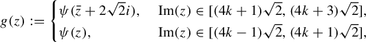 $$ \begin{align*} g(z):= \begin{cases} \psi(\bar{z}+2 \sqrt2i),&\hspace{1mm}{\operatorname{Im}}(z)\in[(4k+1)\sqrt2,(4k+3)\sqrt2],\\\psi(z),&\hspace{1mm}{\operatorname{Im}}(z)\in[(4k-1)\sqrt2,(4k+1)\sqrt2], \end{cases} \end{align*} $$
where $k\in \mathbb {Z}$
and
$k\in \mathbb {Z}$
and $\psi (x+iy)= \nu e^{\lambda x}(\mathfrak {h}_3({y}/{\sqrt 2},{y}/{\sqrt 2})+i\sqrt 2\mathfrak {h}_1({y}/{\sqrt 2},{y}/{\sqrt 2}))$
. Similarly, the Zorich map is conjugate to a similar map to g on the plane
$\psi (x+iy)= \nu e^{\lambda x}(\mathfrak {h}_3({y}/{\sqrt 2},{y}/{\sqrt 2})+i\sqrt 2\mathfrak {h}_1({y}/{\sqrt 2},{y}/{\sqrt 2}))$
. Similarly, the Zorich map is conjugate to a similar map to g on the plane $x_2=-x_1$
and everything that follows works in that case as well. For simplicity let us write
$x_2=-x_1$
and everything that follows works in that case as well. For simplicity let us write $a(y)$
and
$a(y)$
and $b(y)$
instead of
$b(y)$
instead of $\mathfrak {h}_3(y/\sqrt 2,y/\sqrt 2)$
and
$\mathfrak {h}_3(y/\sqrt 2,y/\sqrt 2)$
and $\sqrt 2\mathfrak {h}_1(y/\sqrt 2,y/\sqrt 2)$
. Note that
$\sqrt 2\mathfrak {h}_1(y/\sqrt 2,y/\sqrt 2)$
. Note that $a^2(y)+b^2(y)=1$
. Also let us note here that the function
$a^2(y)+b^2(y)=1$
. Also let us note here that the function $\psi $
is quasiregular and that
$\psi $
is quasiregular and that $g(\mathbb {C})=\{{\operatorname {Re}}\ z>0 \}$
. Furthermore, g is not a quasiregular map, since it is not sense preserving, and is a two-to-one function in the strip
$g(\mathbb {C})=\{{\operatorname {Re}}\ z>0 \}$
. Furthermore, g is not a quasiregular map, since it is not sense preserving, and is a two-to-one function in the strip $\{z\in \mathbb {C}:(4k-1)\sqrt 2\leq {\operatorname {Im}}(z)\leq (4k+3)\sqrt 2\}$
.
$\{z\in \mathbb {C}:(4k-1)\sqrt 2\leq {\operatorname {Im}}(z)\leq (4k+3)\sqrt 2\}$
.
We would now like to show that the planes $x_1=\pm x_2$
belong to the Julia set of
$x_1=\pm x_2$
belong to the Julia set of $\mathcal {Z}_{\nu }$
. We already know, from Proposition 1, that the
$\mathcal {Z}_{\nu }$
. We already know, from Proposition 1, that the $x_3$
-axis belongs to the Julia set. With that in mind we will prove that any open set in
$x_3$
-axis belongs to the Julia set. With that in mind we will prove that any open set in $\mathbb {R}^3$
that intersects those planes also intersects the
$\mathbb {R}^3$
that intersects those planes also intersects the $x_3$
-axis under iteration by
$x_3$
-axis under iteration by $\mathcal {Z}_\nu $
. Now since we know that
$\mathcal {Z}_\nu $
. Now since we know that $\mathcal {Z}_{\nu }$
is conjugate to g on those planes it is enough to prove that any open set in the complex plane intersects the real axis under iteration by g.
$\mathcal {Z}_{\nu }$
is conjugate to g on those planes it is enough to prove that any open set in the complex plane intersects the real axis under iteration by g.
Theorem 5 Let $\nu ^2\lambda>2L$
and
$\nu ^2\lambda>2L$
and $V\subset \mathbb {C}$
be a connected set with
$V\subset \mathbb {C}$
be a connected set with $m(V)>0$
, where m is the two-dimensional Lebesgue measure. Then
$m(V)>0$
, where m is the two-dimensional Lebesgue measure. Then $g^n(V)$
intersects the real axis for some
$g^n(V)$
intersects the real axis for some $n\in \mathbb {N}$
.
$n\in \mathbb {N}$
.
For the proof of this theorem we will need several lemmas. Note here that since $\mathfrak {h}$
is a Lipschitz function it will also be differentiable almost everywhere. This implies that g is differentiable almost everywhere (a.e.).
$\mathfrak {h}$
is a Lipschitz function it will also be differentiable almost everywhere. This implies that g is differentiable almost everywhere (a.e.).
Lemma 2 Let $g$
be the function we defined above. Then
$g$
be the function we defined above. Then
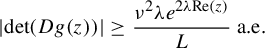 $$ \begin{align*} |\!\det (Dg(z))|\geq\frac{\nu^2\lambda e^{2\lambda{\operatorname{Re}}(z)}}{L}\ \text{a.e.} \end{align*} $$
Proof. It is enough to find a lower bound for ${\operatorname {Im}}\ z\in [(4k-1)\sqrt 2,(4k+1)\sqrt 2]$
. This is true because for other z we have that
${\operatorname {Im}}\ z\in [(4k-1)\sqrt 2,(4k+1)\sqrt 2]$
. This is true because for other z we have that $T(z)=\bar {z}+2\sqrt 2 i$
has imaginary part in
$T(z)=\bar {z}+2\sqrt 2 i$
has imaginary part in $[(4k'-1)\sqrt 2,(4k'+1)\sqrt 2]$
for some
$[(4k'-1)\sqrt 2,(4k'+1)\sqrt 2]$
for some $k'\in \mathbb {Z}$
and thus for those z we have
$k'\in \mathbb {Z}$
and thus for those z we have $g(z)=g(T(z))=\psi (T(z))$
. Then by the chain rule we have that
$g(z)=g(T(z))=\psi (T(z))$
. Then by the chain rule we have that $Dg(z)=Dg(T(z))DT(z)$
. Since
$Dg(z)=Dg(T(z))DT(z)$
. Since $DT(z)=-1$
this implies that
$DT(z)=-1$
this implies that $|\!\det Dg(z)|=|\!\det Dg(T(z))|$
.
$|\!\det Dg(z)|=|\!\det Dg(T(z))|$
.
With that in mind, if $z=x+iy$
we have that
$z=x+iy$
we have that $Dg(z)$
is the linear transformation induced by the matrix
$Dg(z)$
is the linear transformation induced by the matrix
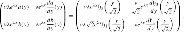 $$ \begin{align*} \begin{pmatrix} \nu\lambda e^{\lambda x}a(y)& \nu e^{\lambda x} \dfrac{da}{dy}({y})\\[12pt] \nu\lambda e^{\lambda x}b(y)& \nu e^{\lambda x} \dfrac{db}{dy}(y) \end{pmatrix}=\begin{pmatrix} \nu\lambda e^{\lambda x}\mathfrak{h}_3\bigg(\dfrac{y}{\sqrt2}\bigg)& \dfrac{\nu}{\sqrt2} e^{\lambda x} \dfrac{d\mathfrak{h}_3}{dy}\bigg(\dfrac{y}{\sqrt2}\bigg)\\[12pt] \nu\lambda\sqrt2 e^{\lambda x}\mathfrak{h}_1\bigg(\dfrac{y}{\sqrt2}\bigg)& \nu e^{\lambda x} \dfrac{d\mathfrak{h}_1}{dy}\bigg(\dfrac{y}{\sqrt2}\bigg) \end{pmatrix}, \end{align*} $$ $\hspace {1mm}\text {if}\hspace {1mm} y\in [(4k-1)\sqrt 2,(4k+1)\sqrt 2]$
.
$\hspace {1mm}\text {if}\hspace {1mm} y\in [(4k-1)\sqrt 2,(4k+1)\sqrt 2]$
.
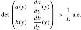
Thus
 $$ \begin{align*}|\!\det Dg(z)|&=\nu^2\lambda e^{2\lambda x}\bigg|\mathfrak{h}_3(y)\dfrac{d\mathfrak{h}_1}{dy}(y)-\mathfrak{h}_1(y)\dfrac{d\mathfrak{h}_3}{dy}(y)\bigg|\\ &=\nu^2\lambda e^{2\lambda x} \left|\det\begin{pmatrix} a(y)& \dfrac{da}{dy}({y})\\[8pt] b(y)& \dfrac{db}{dy}(y)\end{pmatrix}\right|\quad\text{for } y\in[(4k-1)\sqrt2,(4k+1)\sqrt2].\end{align*} $$
We now claim that
 $$ \begin{align*} \left|\det\begin{pmatrix} a(y)& \dfrac{da}{dy}({y})\\[8pt] b(y)& \dfrac{db}{dy}(y)\end{pmatrix}\right|>\dfrac{1}{L}\ \text{a.e.}\end{align*} $$
Hence
 $$ \begin{align*}|\!\det Dg(z)|\geq\dfrac{\nu^2\lambda e^{2\lambda x}}{L}\ \text{a.e.}\end{align*} $$
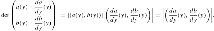
Indeed, because $a^2(y)+b^2(y)=1$
we obtain that the vectors
$a^2(y)+b^2(y)=1$
we obtain that the vectors $(a(y),b(y))$
and
$(a(y),b(y))$
and $({da}/{dy},{db}/{dy})$
are orthogonal and thus so is their matrix. This implies that
$({da}/{dy},{db}/{dy})$
are orthogonal and thus so is their matrix. This implies that
 $$ \begin{align*} \left|\det\begin{pmatrix} a(y)& \dfrac{da}{dy}({y})\\[8pt] b(y)& \dfrac{db}{dy}(y)\end{pmatrix}\right|=|(a(y),b(y))|\bigg|\bigg(\dfrac{da}{dy}({y}), \dfrac{db}{dy}({y})\bigg)\bigg|=\bigg|\bigg(\dfrac{da}{dy}({y}),\dfrac{db}{dy}({y})\bigg)\bigg|.\end{align*} $$
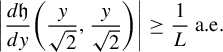
Now because $\mathfrak {h}$
is a locally bi-Lipschitz map almost everywhere we have that
$\mathfrak {h}$
is a locally bi-Lipschitz map almost everywhere we have that
 $$ \begin{align*}\bigg|\frac{d\mathfrak{h}}{dy}\bigg(\frac{y}{\sqrt2},\frac{y}{\sqrt2}\bigg)\bigg|\geq \frac{1}{L}\ \text{a.e.}\end{align*} $$
Since $|({da}/{dy})({y}),({db}/{dy})(y)|=|({d\mathfrak {h}}/{dy})({y}/{\sqrt 2},{y}/{\sqrt 2})|$
we obtain what we wanted.
$|({da}/{dy})({y}),({db}/{dy})(y)|=|({d\mathfrak {h}}/{dy})({y}/{\sqrt 2},{y}/{\sqrt 2})|$
we obtain what we wanted.
Lemma 3 Let $\nu ^2\lambda>2L$
where
$\nu ^2\lambda>2L$
where $\lambda \geq 1$
,
$\lambda \geq 1$
, $\nu>0$
, and let
$\nu>0$
, and let $V\subset \mathbb {C}$
be a connected subset of the complex plane with
$V\subset \mathbb {C}$
be a connected subset of the complex plane with $m(V)>0$
and such that its iterates under g do not intersect the real axis. Then
$m(V)>0$
and such that its iterates under g do not intersect the real axis. Then $m(g^n(V))\to \infty $
as
$m(g^n(V))\to \infty $
as $n\to \infty $
, where m is the two-dimensional Lebesgue measure.
$n\to \infty $
, where m is the two-dimensional Lebesgue measure.
Proof. We can assume that V lies on the right half-plane $\{z:{\operatorname {Re}}(z)>0\}$
, otherwise just consider
$\{z:{\operatorname {Re}}(z)>0\}$
, otherwise just consider $g(V)$
since g maps
$g(V)$
since g maps $\mathbb {C}$
to the right half-plane. We know that
$\mathbb {C}$
to the right half-plane. We know that $m(g(V))=\int _{g(V)}\,dm$
. Since none of the iterates of V under g intersects the real axis, we have that those iterates also do not intersect any of the pre-images of the real axis, meaning the lines
$m(g(V))=\int _{g(V)}\,dm$
. Since none of the iterates of V under g intersects the real axis, we have that those iterates also do not intersect any of the pre-images of the real axis, meaning the lines $y=2\sqrt 2k$
,
$y=2\sqrt 2k$
, $k\in ~\mathbb {Z}$
. Thus
$k\in ~\mathbb {Z}$
. Thus $g^n(V)$
is always inside strips of the form
$g^n(V)$
is always inside strips of the form ${\{z\in \mathbb {C}:{\operatorname {Im}}\ z\in (2\sqrt 2k,2\sqrt 2(k+1))\}}$
. In each of those strips it is easy to see, by what we have said in the first paragraph of this section, that g is a two-to-one map. By using Lemma 2 and since
${\{z\in \mathbb {C}:{\operatorname {Im}}\ z\in (2\sqrt 2k,2\sqrt 2(k+1))\}}$
. In each of those strips it is easy to see, by what we have said in the first paragraph of this section, that g is a two-to-one map. By using Lemma 2 and since ${\operatorname {Re}}\ z>0$
for all
${\operatorname {Re}}\ z>0$
for all $z\in V$
we now obtain
$z\in V$
we now obtain
 $$ \begin{align*} \int_{g(V)}\,dm\geq\frac{1}{2}\int_V |\!\det (Dg)|\,dm\geq\frac{\nu^2\lambda}{2L} \int_V e^{2\lambda{\operatorname{Re}}(z)}\,dm\geq \frac{\nu^2\lambda}{2L}m(V). \end{align*} $$
This means that
 $$ \begin{align*} m(g(V))\geq \frac{\nu^2\lambda }{2L}m(V). \end{align*} $$
Hence, since $\nu ^2\lambda>2L$
, if we iterate that inequality we have that
$\nu ^2\lambda>2L$
, if we iterate that inequality we have that $m(g^n(V))\to \infty $
.
$m(g^n(V))\to \infty $
.
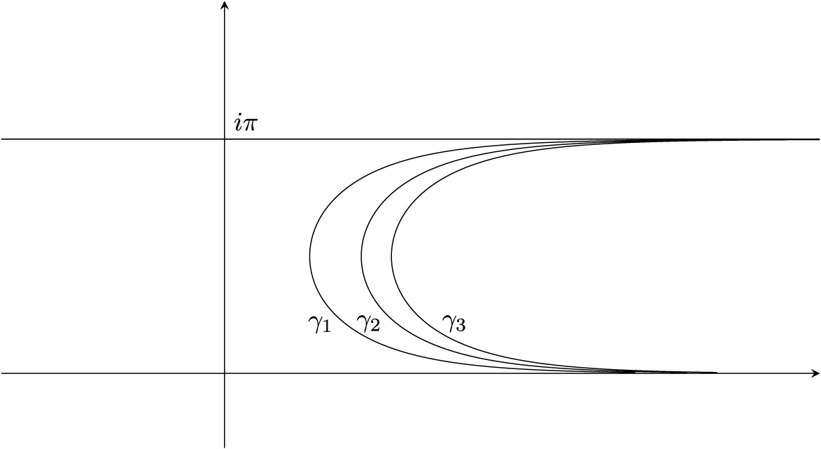
Figure 1 The pre-images of the lines $2k\pi i$
,
$2k\pi i$
, $k\in \mathbb {Z}\setminus \{0\}$
under the exponential map. The curves
$k\in \mathbb {Z}\setminus \{0\}$
under the exponential map. The curves $\gamma _m$
in the proof of Theorem 5 have a similar structure.
$\gamma _m$
in the proof of Theorem 5 have a similar structure.
Proof Proof of Theorem 5
Suppose, towards a contradiction, that there is a connected set V with $m(V)>0$
whose iterates never intersect the real axis. Then by Lemma 3 we have that
$m(V)>0$
whose iterates never intersect the real axis. Then by Lemma 3 we have that $m(g^n(V))\to \infty $
as
$m(g^n(V))\to \infty $
as $n\to \infty $
. Since
$n\to \infty $
. Since $g^n(V)$
never intersects the real axis it also does not intersect its pre-images, meaning the lines
$g^n(V)$
never intersects the real axis it also does not intersect its pre-images, meaning the lines ${\operatorname {Im}}(z)=2\sqrt 2k$
,
${\operatorname {Im}}(z)=2\sqrt 2k$
, $k\in \mathbb {Z}$
. This means that
$k\in \mathbb {Z}$
. This means that $g^n(V)$
stays always inside strips of the form
$g^n(V)$
stays always inside strips of the form $\{ z\in \mathbb {C}:{\operatorname {Im}}(z)\in (2\sqrt 2k,2\sqrt 2(k+1)),k\in \mathbb {Z}\}$
. If we now take the pre-image of the lines
$\{ z\in \mathbb {C}:{\operatorname {Im}}(z)\in (2\sqrt 2k,2\sqrt 2(k+1)),k\in \mathbb {Z}\}$
. If we now take the pre-image of the lines ${\operatorname {Im}}(z)=2\sqrt 2m$
,
${\operatorname {Im}}(z)=2\sqrt 2m$
, $m\in \mathbb {Z}\setminus \{0\}$
, that lie inside all those strips we obtain curves
$m\in \mathbb {Z}\setminus \{0\}$
, that lie inside all those strips we obtain curves $\gamma _m$
which the iterates
$\gamma _m$
which the iterates $g^n(V)$
of our set must not cross (see Figure 1). By symmetry we can confine ourselves to the strip
$g^n(V)$
of our set must not cross (see Figure 1). By symmetry we can confine ourselves to the strip
 $$ \begin{align*} S:=\{ z\in\mathbb{C}:{\operatorname{Im}}(z)\in(0,2\sqrt2)\}. \end{align*} $$
From now on let us write $\mathfrak {h}_i(y)$
instead of
$\mathfrak {h}_i(y)$
instead of $\mathfrak {h}_i(y,y)$
,
$\mathfrak {h}_i(y,y)$
, $i=1,2,3$
, for simplicity. We now have two cases to consider. Either S contains the pre-images of the lines
$i=1,2,3$
, for simplicity. We now have two cases to consider. Either S contains the pre-images of the lines ${\operatorname {Im}}(z)=2\sqrt 2m$
,
${\operatorname {Im}}(z)=2\sqrt 2m$
, $m>0$
, in which case
$m>0$
, in which case $\mathfrak {h}_1(y)>0$
for
$\mathfrak {h}_1(y)>0$
for $y>0$
, or S contains the pre-images of the lines for
$y>0$
, or S contains the pre-images of the lines for $m<0$
, in which case
$m<0$
, in which case $\mathfrak {h}_1(y)<0$
for
$\mathfrak {h}_1(y)<0$
for $y>0$
. We will only consider the first case here. The second one can be dealt with similarly. So suppose
$y>0$
. We will only consider the first case here. The second one can be dealt with similarly. So suppose $m>0$
. We claim that the curves
$m>0$
. We claim that the curves $\gamma _m$
partition the strip S into sets of uniformly bounded area. In fact if we call
$\gamma _m$
partition the strip S into sets of uniformly bounded area. In fact if we call $A_m$
the area of the set defined by
$A_m$
the area of the set defined by $\gamma _m$
and
$\gamma _m$
and $\gamma _{m+1}$
and we call
$\gamma _{m+1}$
and we call $A_0$
the area inside the strip between the imaginary axis and
$A_0$
the area inside the strip between the imaginary axis and $\gamma _1$
, then we claim that
$\gamma _1$
, then we claim that $A_m$
is an eventually decreasing sequence. Clearly, since
$A_m$
is an eventually decreasing sequence. Clearly, since $m(g^n(V))\to \infty $
and
$m(g^n(V))\to \infty $
and $g^n(V)$
must stay inside those sets
$g^n(V)$
must stay inside those sets $A_m$
, this is impossible.
$A_m$
, this is impossible.
In order to prove those claims note that the curves $\gamma _m$
are given by the equations
$\gamma _m$
are given by the equations $\nu e^{\lambda x}\mathfrak {h}_1({y}/{\sqrt 2})=2m,$
when
$\nu e^{\lambda x}\mathfrak {h}_1({y}/{\sqrt 2})=2m,$
when $y\in (0,\sqrt 2]$
, and
$y\in (0,\sqrt 2]$
, and $\nu e^{\lambda x}\mathfrak {h}_1(({2\sqrt 2-y})/{\sqrt 2})=2m$
, when
$\nu e^{\lambda x}\mathfrak {h}_1(({2\sqrt 2-y})/{\sqrt 2})=2m$
, when ${y\in [\sqrt 2,2\sqrt 2)}$
. It is also easy to see that those curves do not have self-intersections and do not intersect with each other. The area we are looking for will be given by
${y\in [\sqrt 2,2\sqrt 2)}$
. It is also easy to see that those curves do not have self-intersections and do not intersect with each other. The area we are looking for will be given by
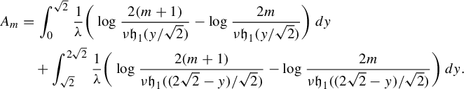 $$ \begin{align*} A_m&=\int_{0}^{\sqrt2}\frac{1}{\lambda}\bigg(\log\frac{2(m+1)}{\nu \mathfrak{h}_1({y}/{\sqrt2})}-\log\frac{2m}{\nu \mathfrak{h}_1({y}/{\sqrt2})}\bigg)\,dy\\ &\quad+\int_{\sqrt2}^{2\sqrt2}\frac{1}{\lambda}\bigg(\log\frac{2(m+1)}{\nu \mathfrak{h}_1 (({2\sqrt2-y})/{\sqrt2})} -\log\frac{2m}{\nu \mathfrak{h}_1(({2\sqrt2-y})/{\sqrt2})}\bigg)\,dy. \end{align*} $$
Thus $A_m=({2\sqrt 2}/{\lambda })\log (({m+1})/{m})$
which proves what we wanted. We also need to find
$A_m=({2\sqrt 2}/{\lambda })\log (({m+1})/{m})$
which proves what we wanted. We also need to find $A_0$
for which it is true that
$A_0$
for which it is true that
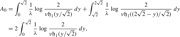 $$ \begin{align*}A_0&=\int_{0}^{\sqrt2}\frac{1}{\lambda}\log \frac{2}{\nu \mathfrak{h}_1({y}/{\sqrt2})}\,dy+\int_{\sqrt2}^{2\sqrt2}\frac{1}{\lambda}\log\frac{2}{\nu \mathfrak{h}_1(({2\sqrt2-y})/{\sqrt2})}\,dy\\ &=2\int_{0}^{\sqrt2}\frac{1}{\lambda}\log \frac{2}{\nu \mathfrak{h}_1({y}/{\sqrt2})}\,dy,\end{align*} $$
if $\nu \mathfrak {h}_1({y}/{\sqrt 2})=2$
has no solution. If this equation has solutions then, although we can find the area again we do not need to since
$\nu \mathfrak {h}_1({y}/{\sqrt 2})=2$
has no solution. If this equation has solutions then, although we can find the area again we do not need to since $A_0$
will be even smaller in this case (see Figure 2).
$A_0$
will be even smaller in this case (see Figure 2).
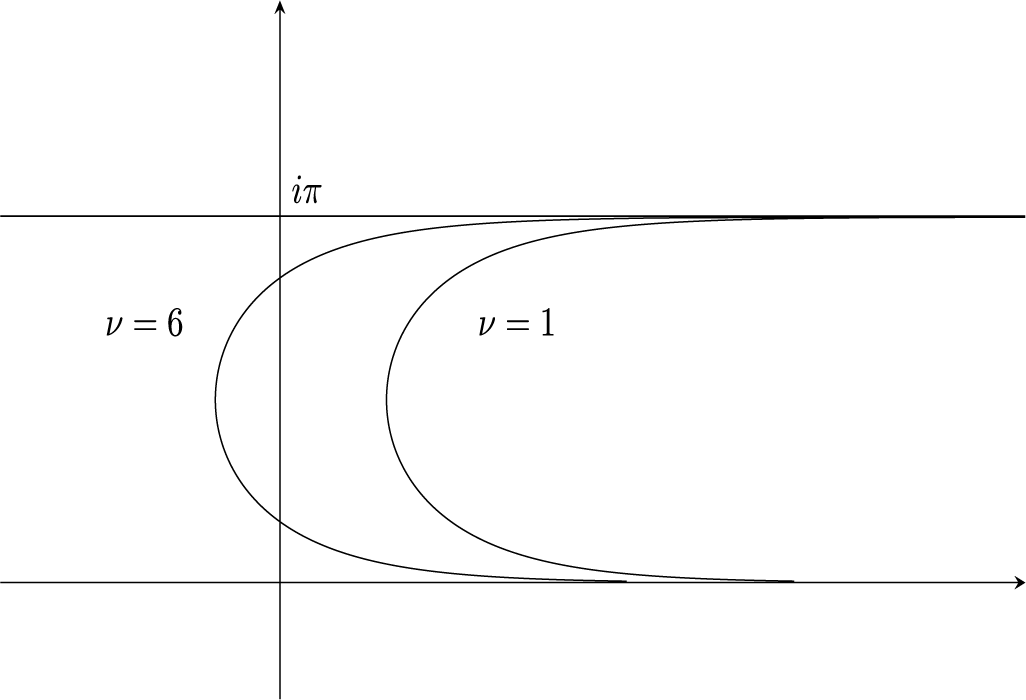
Figure 2 The curve $\gamma _0$
for the exponential map for two different values of
$\gamma _0$
for the exponential map for two different values of $\nu $
. The situation is similar with our maps as well.
$\nu $
. The situation is similar with our maps as well.
Notice that because $(\mathfrak {h}_1,\mathfrak {h}_2,\mathfrak {h}_3)$
is always a point on the unit sphere we have that
$(\mathfrak {h}_1,\mathfrak {h}_2,\mathfrak {h}_3)$
is always a point on the unit sphere we have that
 $$ \begin{align*}\mathfrak{h}_1(x,y)^2+\mathfrak{h}_2(x,y)^2&=\sin^2 \theta|\mathfrak{h}(x,y)-\mathfrak{h}(0,0)|^2\\ &=\sin^2 \theta (\mathfrak{h}_1(x,y)^2+\mathfrak{h}_2(x,y)^2+(\mathfrak{h}_3(x,y)-1)^2),\end{align*} $$
where $\theta $
is the angle between the
$\theta $
is the angle between the $x_3$
-axis and the segment that connects
$x_3$
-axis and the segment that connects $(0,0,1)$
with
$(0,0,1)$
with $(\mathfrak {h}_1,\mathfrak {h}_2,\mathfrak {h}_3)$
. Taking
$(\mathfrak {h}_1,\mathfrak {h}_2,\mathfrak {h}_3)$
. Taking $x=y$
, the fact that
$x=y$
, the fact that $\mathfrak {h}$
is bi-Lipschitz on
$\mathfrak {h}$
is bi-Lipschitz on $[-1,1]^2$
and noticing that
$[-1,1]^2$
and noticing that $\theta \geq \pi /4$
gives us
$\theta \geq \pi /4$
gives us $|\mathfrak {h}_1(y)|\geq ({|y|}/{\sqrt 2L}).$
Hence because
$|\mathfrak {h}_1(y)|\geq ({|y|}/{\sqrt 2L}).$
Hence because $\mathfrak {h}_1(y)>0$
for
$\mathfrak {h}_1(y)>0$
for $y\in (0,1)$
we have
$y\in (0,1)$
we have
 $$ \begin{align*} A_0\leq \frac{2}{\lambda}\int_{0}^{\sqrt2}\log\bigg(\frac{4L}{\nu y}\bigg)\,dy, \end{align*} $$
which is finite.
4 Proof of Theorem 1
Having proved Theorem 5, we are now ready to proceed to our main theorem.
First we prove some lemmas that we will later need. Note here that since we proved that the planes $x_1=\pm x_2$
are in the Julia set of
$x_1=\pm x_2$
are in the Julia set of $\mathcal {Z}_{\nu }$
we will also know that all their inverse images are in the Julia set. These inverse images are again planes of the form
$\mathcal {Z}_{\nu }$
we will also know that all their inverse images are in the Julia set. These inverse images are again planes of the form $x_1=\pm x_2 + 2\lambda k$
, where
$x_1=\pm x_2 + 2\lambda k$
, where $k\in \mathbb {Z}$
. The planes partition
$k\in \mathbb {Z}$
. The planes partition $\mathbb {R}^3$
into square beams. Denote by
$\mathbb {R}^3$
into square beams. Denote by $B_{(0,0)}$
the open rectangle beam that is the union of the two square beams that touch the
$B_{(0,0)}$
the open rectangle beam that is the union of the two square beams that touch the $x_3$
-axis and are in the half-space
$x_3$
-axis and are in the half-space $x_2\leq x_1$
. We can partition the space now into rectangle beams that are translates of this
$x_2\leq x_1$
. We can partition the space now into rectangle beams that are translates of this $B_{(0,0)}$
. Let us call them
$B_{(0,0)}$
. Let us call them
 $$ \begin{align*} B_{(i,j)}=B_{(0,0)}+i(2\lambda,2\lambda,0)+j(\lambda,-\lambda,0), \quad i,j\in\mathbb{Z}. \end{align*} $$
Note that the map $\mathcal {Z}_{\nu }$
is a homeomorphism in those rectangle beams. The next lemma is inspired by the one Misiurewicz used in his proof (compare [Reference Misiurewicz23, Lemma 1]) and is the main reason why we need the scale factor
$\mathcal {Z}_{\nu }$
is a homeomorphism in those rectangle beams. The next lemma is inspired by the one Misiurewicz used in his proof (compare [Reference Misiurewicz23, Lemma 1]) and is the main reason why we need the scale factor $\lambda $
in our definition of the Zorich map. It will be convenient to introduce some notation. Let
$\lambda $
in our definition of the Zorich map. It will be convenient to introduce some notation. Let $p:\mathbb {R}^3\to \mathbb {R}^2$
be the projection map defined by
$p:\mathbb {R}^3\to \mathbb {R}^2$
be the projection map defined by $p(x_1,x_2,x_3)=(x_1,x_2)$
. Also let
$p(x_1,x_2,x_3)=(x_1,x_2)$
. Also let $p_3(x)$
,
$p_3(x)$
, $x\in \mathbb {R}^3$
, denote the third coordinate of x; in other words,
$x\in \mathbb {R}^3$
, denote the third coordinate of x; in other words, $p_3(x_1,x_2,x_3)=x_3$
.
$p_3(x_1,x_2,x_3)=x_3$
.
Lemma 4 If $\lambda $
and L are the numbers we used in the construction of the Zorich map and
$\lambda $
and L are the numbers we used in the construction of the Zorich map and $\nu>0$
then
$\nu>0$
then
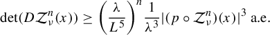 $$ \begin{align*} \det(D\mathcal{Z}_{\nu}^n(x))\geq {\bigg(\frac{\lambda }{L^5}\bigg)}^{n}\frac{1}{\lambda^{3}}|( p \circ \mathcal{Z}_{\nu}^{n})(x)|^3\ \text{a.e.}\end{align*} $$
Proof. First note that $|p(\mathcal {Z}_{\nu }^n(x))|=\nu e^{p_3(\mathcal {Z}_{\nu }^{n-1})}\cdot |(p\circ h\circ p\circ \mathcal {Z}_{\nu }^{n-1})(x) |$
. Also, using the fact that
$|p(\mathcal {Z}_{\nu }^n(x))|=\nu e^{p_3(\mathcal {Z}_{\nu }^{n-1})}\cdot |(p\circ h\circ p\circ \mathcal {Z}_{\nu }^{n-1})(x) |$
. Also, using the fact that $h(0)=(0,0,\lambda )$
and
$h(0)=(0,0,\lambda )$
and $h(x_1,x_2)=(h_1(x_1,x_2),h_2(x_1,x_2),h_3(x_1,x_2))$
is a Lipschitz map, we have that
$h(x_1,x_2)=(h_1(x_1,x_2),h_2(x_1,x_2),h_3(x_1,x_2))$
is a Lipschitz map, we have that
 $$ \begin{align*} |p(h(x))|=|p(h(x)-h(0))|\leq|h(x)-h(0)|\leq L|x|. \end{align*} $$
Hence
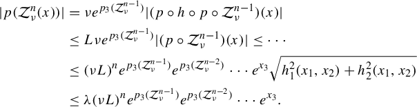 $$ \begin{align} |p(\mathcal{Z}_{\nu}^n(x))|&=\nu e^{p_3(\mathcal{Z}_{\nu}^{n-1})}|(p\circ h\circ p \circ \mathcal{Z}_{\nu}^{n-1})(x)|\nonumber\\ &\leq L\nu e^{p_3(\mathcal{Z}_{\nu}^{n-1})}|( p \circ \mathcal{Z}_{\nu}^{n-1})(x)|\leq\cdots\nonumber\\ &\leq (\nu L)^{n}e^{p_3(\mathcal{Z}_{\nu}^{n-1})}e^{p_3(\mathcal{Z}_{\nu}^{n-2})}\cdots e^{x_3}\sqrt{h_1^2 (x_1,x_2 )+h_2^2 (x_1,x_2 )}\nonumber\\ &\leq \lambda (\nu L)^{n}e^{p_3(\mathcal{Z}_{\nu}^{n-1})}e^{p_3(\mathcal{Z}_{\nu}^{n-2})}\cdots e^{x_3}. \end{align} $$
From the chain rule we know that
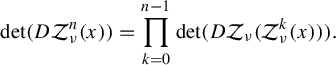 $$ \begin{align}\det(D\mathcal{Z}_{\nu}^n(x))=\prod_{k=0}^{n-1}\det(D\mathcal{Z}_{\nu}({\mathcal{Z}_{\nu}^{k}(x)})).\end{align} $$
Now from the definition of $\mathcal {Z}_{\nu }$
we obtain
$\mathcal {Z}_{\nu }$
we obtain
 $$ \begin{align}\det(D\mathcal{Z}_{\nu}(x))=\nu^3 e^{3x_3}\det H,\end{align} $$
where
 $$ \begin{align*}H=\begin{pmatrix} \dfrac{\partial h_1}{\partial x_1}(p(x))&\dfrac{\partial h_1}{\partial x_2}(p(x))&h_1(p(x))\\ \dfrac{\partial h_2}{\partial x_1}(p(x))&\dfrac{\partial h_2}{\partial x_2}(p(x))&h_2(p(x))\\ \dfrac{\partial h_3}{\partial x_1}(p(x))&\dfrac{\partial h_3}{\partial x_2}(p(x))&h_3(p(x)) \end{pmatrix}.\end{align*} $$
We now set
 $$ \begin{align*} A=\begin{pmatrix} \dfrac{\partial h_1}{\partial x_1}(p(x))\\[10pt] \dfrac{\partial h_2}{\partial x_1}(p(x))\\[10pt] \dfrac{\partial h_3}{\partial x_1}(p(x)) \end{pmatrix},\quad B=\begin{pmatrix} \dfrac{\partial h_1}{\partial x_2}(p(x))\\[10pt] \dfrac{\partial h_2}{\partial x_2}(p(x))\\[10pt] \dfrac{\partial h_3}{\partial x_2}(p(x))\end{pmatrix},\quad C=\begin{pmatrix} h_1(p(x))\\ h_2(p(x))\\h_3(p(x)) \end{pmatrix}. \end{align*} $$
Recall now that from linear algebra, the determinant of a matrix equals the scalar triple product. This means that
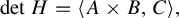 $$ \begin{align*} \det H=\langle A\times B, C\rangle, \end{align*} $$
where $\langle \cdot ,\cdot \rangle $
denotes the euclidean inner product. Since
$\langle \cdot ,\cdot \rangle $
denotes the euclidean inner product. Since $\mathcal {Z}_{\nu }$
is sense preserving we will have that
$\mathcal {Z}_{\nu }$
is sense preserving we will have that $\det H>0$
, and since A and B are orthogonal to C we will have that
$\det H>0$
, and since A and B are orthogonal to C we will have that $A\times B$
is parallel to C. Remember that
$A\times B$
is parallel to C. Remember that $|C|=\lambda $
, so
$|C|=\lambda $
, so
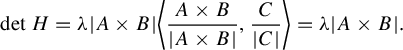 $$ \begin{align} \det H= \lambda|A\times B| \bigg\langle \frac{A\times B}{|A\times B|}, \frac{C}{|C|}\bigg\rangle= \lambda |A\times B|.\end{align} $$
Now because $\mathfrak {h}$
is a locally bi-Lipschitz map we have that
$\mathfrak {h}$
is a locally bi-Lipschitz map we have that
 $$ \begin{align*} |h(p(x)+tv)-h(p(x))|\geq\frac{|tv|}{L}, \end{align*} $$
for all small $t>0$
where
$t>0$
where $v=(v_1,v_2)\in \mathbb {R}^2$
. This implies that
$v=(v_1,v_2)\in \mathbb {R}^2$
. This implies that
 $$ \begin{align} |Dh(p(x))(v)|\geq \frac{|v|}{L}, \end{align} $$
and if we set $v=(|B|,({-\langle A,B\rangle })/{|B|})$
and square both sides we obtain
$v=(|B|,({-\langle A,B\rangle })/{|B|})$
and square both sides we obtain
 $$ \begin{align*} \bigg| |B|A-\frac{\langle A,B\rangle}{|B|}B\bigg|^2\geq \frac{1}{L^2}\bigg(|B|^2+\frac{\langle A,B\rangle^2}{|B|^2}\bigg)\geq\frac{|B|^2}{L^2}. \end{align*} $$
Simplifying, we obtain
 $$ \begin{align*} |A|^2|B|^2-\langle A,B\rangle^2\geq\frac{|B|^2}{L^2}. \end{align*} $$
Now note that, by elementary properties of the cross product, $|A\times B|^2=|A|^2|B|^2-\langle A,B\rangle ^2$
and thus
$|A\times B|^2=|A|^2|B|^2-\langle A,B\rangle ^2$
and thus
 $$ \begin{align*}|A\times B|^2\geq \frac{|B|^2}{L^2}\geq \frac{1}{L^4},\end{align*} $$
where the last inequality comes from (4.5) for $v=(0,1)$
. Hence, (4.4) becomes
$v=(0,1)$
. Hence, (4.4) becomes $\det H\geq ({\lambda }/{L^2})$
. Putting everything together in (4.3), we obtain
$\det H\geq ({\lambda }/{L^2})$
. Putting everything together in (4.3), we obtain
 $$ \begin{align}\det(D\mathcal{Z}_{\nu}(x))\geq \nu^3 e^{3x_3}\frac{\lambda}{L^2}\ \text{a.e.}\end{align} $$
Hence, by (4.1) and (4.6) we have that
 $$ \begin{align*}|p(\mathcal{Z}_{\nu}^n(x))|^3&\leq\lambda^3 (L\nu)^{3n}e^{3p_3(\mathcal{Z}_{\nu}^{n-1})}e^{3p_3(\mathcal{Z}_{\nu}^{n-2})}\cdots e^{3x_3}\\ &\leq\frac{\lambda^3 L^{5n}}{\lambda^{n}}\det(D\mathcal{Z}_{\nu}(\mathcal{Z}_{\nu}^{n-1}(x)))\cdots\det(D\mathcal{Z}_{\nu}(x)) \ \text{a.e}.\end{align*} $$
By rearranging and (4.2) we now obtain the desired inequality.
The next lemma describes the behaviour of points near the $x_3$
-axis under iteration.
$x_3$
-axis under iteration.
Lemma 5 Let $\nu \lambda>({1}/{e}).$
-
(a) There are
$\delta>0$
and
$c>0$
such that if
$x\in C_{\delta }$
, where
$C_{\delta }$
is the cylinder around the
$x_3$
-axis with radius
$\delta $
, then
$p_3(\mathcal {Z}_{\nu }(x))>p_3(x)+c$
, -
(b) For
$\delta $
as in (a) and for every
$x\in C_{\delta }$
, with
$p(x)\not =(0,0)$
, there is an
$n\in \mathbb {N}$
such that
$\mathcal {Z}_{\nu }^n(x)\not \in C_{\delta }$
.


Proof. (a) If $h(x_1,x_2)=(h_1(x_1,x_2),h_2(x_1,x_2),h_3(x_1,x_2))$
, then we have that
$h(x_1,x_2)=(h_1(x_1,x_2),h_2(x_1,x_2),h_3(x_1,x_2))$
, then we have that $p_3(\mathcal {Z}_{\nu }(x))=\nu e^{x_3}h_3(x_1,x_2)$
. Now since
$p_3(\mathcal {Z}_{\nu }(x))=\nu e^{x_3}h_3(x_1,x_2)$
. Now since $h(0,0)=(0,0,\lambda )$
and h is continuous, for all
$h(0,0)=(0,0,\lambda )$
and h is continuous, for all $\varepsilon>0$
there is a disk
$\varepsilon>0$
there is a disk $D=D(0,\delta )$
of radius
$D=D(0,\delta )$
of radius $\delta>0$
on which we have
$\delta>0$
on which we have $h_3(x_1,x_2)>\lambda -\varepsilon $
. Hence if
$h_3(x_1,x_2)>\lambda -\varepsilon $
. Hence if $x=(x_1,x_2,x_3)\in C_{\delta }=D\times \mathbb {R}$
, then
$x=(x_1,x_2,x_3)\in C_{\delta }=D\times \mathbb {R}$
, then
 $$ \begin{align*}p_3(\mathcal{Z}_{\nu}(x))=\nu e^{x_3}h_3(x_1,x_2)> \nu e^{p_3(x)}(\lambda-\varepsilon)\geq p_3(x)+1+\log (\nu(\lambda-\varepsilon)),\end{align*} $$
where the last inequality follows by minimizing $\nu e^t(\lambda -\varepsilon )-t$
. Now notice that since
$\nu e^t(\lambda -\varepsilon )-t$
. Now notice that since $\nu \lambda>({1}/{e})$
we can find a small enough
$\nu \lambda>({1}/{e})$
we can find a small enough $\varepsilon>0$
such that
$\varepsilon>0$
such that $\nu (\lambda -\varepsilon )>{1}/{e}$
, which implies that
$\nu (\lambda -\varepsilon )>{1}/{e}$
, which implies that $1+\log (\nu (\lambda -\varepsilon ))>0$
. Hence,
$1+\log (\nu (\lambda -\varepsilon ))>0$
. Hence, $p_3(\mathcal {Z}_{\nu }(x))>p_3(x)+c$
with
$p_3(\mathcal {Z}_{\nu }(x))>p_3(x)+c$
with $c= 1+\log (\nu (\lambda -\varepsilon ))$
.
$c= 1+\log (\nu (\lambda -\varepsilon ))$
.
(b) For a $\delta $
as in (a) and
$\delta $
as in (a) and $\delta <\lambda $
now assume that there is a point
$\delta <\lambda $
now assume that there is a point $x\in C_{\delta }$
such that
$x\in C_{\delta }$
such that $p(x)\not =0$
and
$p(x)\not =0$
and $\mathcal {Z}_{\nu }^n(x)\in C_{\delta }$
for all
$\mathcal {Z}_{\nu }^n(x)\in C_{\delta }$
for all $n\in \mathbb {N}$
. Then according to (a) we would have that
$n\in \mathbb {N}$
. Then according to (a) we would have that $p_3(\mathcal {Z}_{\nu }^n(x))\to \infty $
when
$p_3(\mathcal {Z}_{\nu }^n(x))\to \infty $
when $n\to \infty $
. We know that
$n\to \infty $
. We know that
 $$ \begin{align}|(p\circ \mathcal{Z}_{\nu}^{n+1})(x)|=e^{p_3(\mathcal{Z}_{\nu}^n)}|(p\circ h\circ p\circ\mathcal{Z}_{\nu}^n)(x)|.\end{align} $$
Now its a simple geometric fact that, for each $y\in [-\lambda ,\lambda ]^2$
,
$y\in [-\lambda ,\lambda ]^2$
,
 $$ \begin{align}|(p\circ h)(y)|=\sin \theta |h(y)-h(0)|,\end{align} $$
where $\theta $
is the angle between the line segment joining the point
$\theta $
is the angle between the line segment joining the point $h(y)$
, on the sphere, with the point
$h(y)$
, on the sphere, with the point $(0,0,\lambda )$
and the
$(0,0,\lambda )$
and the $x_3$
-axis. Moreover,
$x_3$
-axis. Moreover, $\theta \geq \pi /4$
for all such y. Also, by the fact that h is a bi-Lipschitz function, we have that
$\theta \geq \pi /4$
for all such y. Also, by the fact that h is a bi-Lipschitz function, we have that $|h(y)-h(0)|\geq ({|y|}/{L}).$
Now taking $y=p(\mathcal {Z}_{\nu }^n(x))$
and combining this with (4.7) and (4.8) implies that
$y=p(\mathcal {Z}_{\nu }^n(x))$
and combining this with (4.7) and (4.8) implies that
 $$ \begin{align*}|(p\circ \mathcal{Z}_{\nu}^{n+1})(x)|\geq \frac{e^{p_3(\mathcal{Z}^n(x))}}{\sqrt2 L}|(p\circ\mathcal{Z}_{\nu}^n)(x)|.\end{align*} $$
Thus, since $p_3(\mathcal {Z}_{\nu }^n(x))\to \infty $
, for all large enough n we can say that
$p_3(\mathcal {Z}_{\nu }^n(x))\to \infty $
, for all large enough n we can say that
 $$ \begin{align*}|(p\circ\mathcal{Z}_{\nu}^{n+1})(x)|\geq2|(p\circ\mathcal{Z}_{\nu}^n)(x)|.\end{align*} $$
This of course contradicts the fact that $\mathcal {Z}^n(x)\in C_{\delta }$
for all
$\mathcal {Z}^n(x)\in C_{\delta }$
for all $n\in \mathbb {N}$
.
$n\in \mathbb {N}$
.
The next lemmas describe how sets of positive measure behave under iteration by the Zorich map, assuming that their iterates never cross the planes that we already know belong in the Julia set.
Lemma 6 Assume that $\lambda>L^{5}$
. Let
$\lambda>L^{5}$
. Let $V\subset \mathbb {R}^3$
be a connected set with
$V\subset \mathbb {R}^3$
be a connected set with $m(V)>0$
and whose iterates do not intersect any of the planes
$m(V)>0$
and whose iterates do not intersect any of the planes $x_1=\pm x_2 + 2\lambda k$
, where
$x_1=\pm x_2 + 2\lambda k$
, where $k\in \mathbb {Z}$
. Suppose also that there is sequence of integers
$k\in \mathbb {Z}$
. Suppose also that there is sequence of integers $n_j>0$
with
$n_j>0$
with $\mathcal {Z}_{\nu }^{n_j}(V)\cap C_a=\emptyset $
, where
$\mathcal {Z}_{\nu }^{n_j}(V)\cap C_a=\emptyset $
, where $C_a$
is a cylinder around the
$C_a$
is a cylinder around the $x_3$
-axis of any radius
$x_3$
-axis of any radius $a>0$
. Then
$a>0$
. Then $m(\mathcal {Z}_{\nu }^{n_j}(V))\to \infty $
as
$m(\mathcal {Z}_{\nu }^{n_j}(V))\to \infty $
as $n_j\to \infty $
, where m is the three-dimensional Lebesgue measure.
$n_j\to \infty $
, where m is the three-dimensional Lebesgue measure.
Proof. Since $\mathcal {Z}_{\nu }^{n_j}(V)$
stays outside the cylinder
$\mathcal {Z}_{\nu }^{n_j}(V)$
stays outside the cylinder $C_a$
we have that, for
$C_a$
we have that, for $x\in V$
,
$x\in V$
,
 $$ \begin{align*}|(p\circ \mathcal{Z}_{\nu}^{n_j})(x)|>a.\end{align*} $$
By using Lemma 4 we will now have that
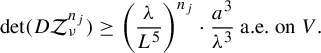 $$ \begin{align*}\det(D\mathcal{Z}_{\nu}^{n_j})\geq{\bigg(\frac{\lambda }{L^5}\bigg)}^{n_j} \cdot \frac{a^3}{\lambda^{3}}\ \text{a.e. on} \ V.\end{align*} $$
Since all of the iterates of V do not intersect any of the planes $x_1=\pm x_2 + 2\lambda k$
, where
$x_1=\pm x_2 + 2\lambda k$
, where $k\in \mathbb {Z}$
, and since the Zorich map is a homeomorphism in the square beams that remain if we remove those planes, we will have that
$k\in \mathbb {Z}$
, and since the Zorich map is a homeomorphism in the square beams that remain if we remove those planes, we will have that $\mathcal {Z}^n$
is a homeomorphism in V. Hence, for all
$\mathcal {Z}^n$
is a homeomorphism in V. Hence, for all $n_j\in \mathbb {N}$
, we will have that
$n_j\in \mathbb {N}$
, we will have that
 $$ \begin{align*}m(\mathcal{Z}_{\nu}^{n_j}(V))=\int_{V}|\!\det(D\mathcal{Z}_{\nu}^{n_j})|\,dm\geq{\bigg(\frac{\lambda }{L^5}\bigg)}^{n_j}{\bigg(\frac{a^3}{\lambda^{3}}\bigg)} m(V),\end{align*} $$
which tends to infinity as $j\to \infty $
since
$j\to \infty $
since $\lambda>{L^{5}}$
.
$\lambda>{L^{5}}$
.
For our next lemma let us assume that our Zorich map sends the beam $B_{(0,0)}$
to the half-space
$B_{(0,0)}$
to the half-space $x_2\leq x_1$
. The other alternative is mapping it to the half-space
$x_2\leq x_1$
. The other alternative is mapping it to the half-space $x_1\leq x_2$
, but the methods work in a very similar way with minor modifications.
$x_1\leq x_2$
, but the methods work in a very similar way with minor modifications.
Consider the inverse image under $\mathcal {Z}_{\nu }$
of the boundary of
$\mathcal {Z}_{\nu }$
of the boundary of $B_{(0,0)}$
that lies in the interior of
$B_{(0,0)}$
that lies in the interior of $B_{(0,0)}$
. This inverse image will be some surface which we will call
$B_{(0,0)}$
. This inverse image will be some surface which we will call $S_0$
. In Figure 3 we have drawn the
$S_0$
. In Figure 3 we have drawn the $x_1 \ x_2$
plane and the rectangle beams
$x_1 \ x_2$
plane and the rectangle beams $B_{(0,0)}$
and
$B_{(0,0)}$
and $B_{(0,-1)}$
. Now take the planes
$B_{(0,-1)}$
. Now take the planes $P_1:x_2=x_1-4\lambda $
,
$P_1:x_2=x_1-4\lambda $
, $P_2:x_2=-x_1+4\lambda $
,
$P_2:x_2=-x_1+4\lambda $
, $P_3: x_2=-x_1-4\lambda $
and consider the rectangle beam they define together with the plane
$P_3: x_2=-x_1-4\lambda $
and consider the rectangle beam they define together with the plane $x_1=x_2$
. Let us now take the boundary of this beam, without the part that belongs to
$x_1=x_2$
. Let us now take the boundary of this beam, without the part that belongs to $x_1=x_2$
, and name it
$x_1=x_2$
, and name it $L_1$
. Consider now the inverse image of
$L_1$
. Consider now the inverse image of $L_1$
that lies inside
$L_1$
that lies inside $B_{(0,0)}$
. This image is a surface; let us call it
$B_{(0,0)}$
. This image is a surface; let us call it $S_1$
. We can now do the same with the planes
$S_1$
. We can now do the same with the planes $P_4:x_2=x_1-6\lambda $
,
$P_4:x_2=x_1-6\lambda $
, $P_5:x_2=-x_1+6\lambda $
,
$P_5:x_2=-x_1+6\lambda $
, $P_6: x_2=-x_1-6\lambda $
and obtain the boundary of the beam they define, which we call
$P_6: x_2=-x_1-6\lambda $
and obtain the boundary of the beam they define, which we call $L_2$
, and then the surface we obtain by taking the inverse image, which we call
$L_2$
, and then the surface we obtain by taking the inverse image, which we call $S_2$
. If we continue with this construction we obtain a sequence of surfaces,
$S_2$
. If we continue with this construction we obtain a sequence of surfaces, $S_0$
,
$S_0$
, $S_1$
,
$S_1$
, $S_2$
,
$S_2$
, $S_3$
,
$S_3$
, $\ldots $
inside
$\ldots $
inside $B_{(0,0)}$
. Each of those surfaces lies above the previous one, starting with
$B_{(0,0)}$
. Each of those surfaces lies above the previous one, starting with $S_0$
. We can also construct similar surfaces
$S_0$
. We can also construct similar surfaces $K_0, K_1, K_2, \ldots $
inside the beam
$K_0, K_1, K_2, \ldots $
inside the beam $B_{(0,-1)}$
by taking inverse images of the corresponding boundaries
$B_{(0,-1)}$
by taking inverse images of the corresponding boundaries $\partial B_{(0,-1)}$
,
$\partial B_{(0,-1)}$
, $R_1$
,
$R_1$
, $R_2$
,
$R_2$
, $\ldots $
(see Figure 3). Moreover, we construct similar surfaces in all the other rectangle beams
$\ldots $
(see Figure 3). Moreover, we construct similar surfaces in all the other rectangle beams $B_{(i,j)}$
, that partition the space, depending on which half-space the beam is mapped to under the Zorich map. Let us denote by
$B_{(i,j)}$
, that partition the space, depending on which half-space the beam is mapped to under the Zorich map. Let us denote by $\mathcal {S}$
the union of all those surfaces.
$\mathcal {S}$
the union of all those surfaces.
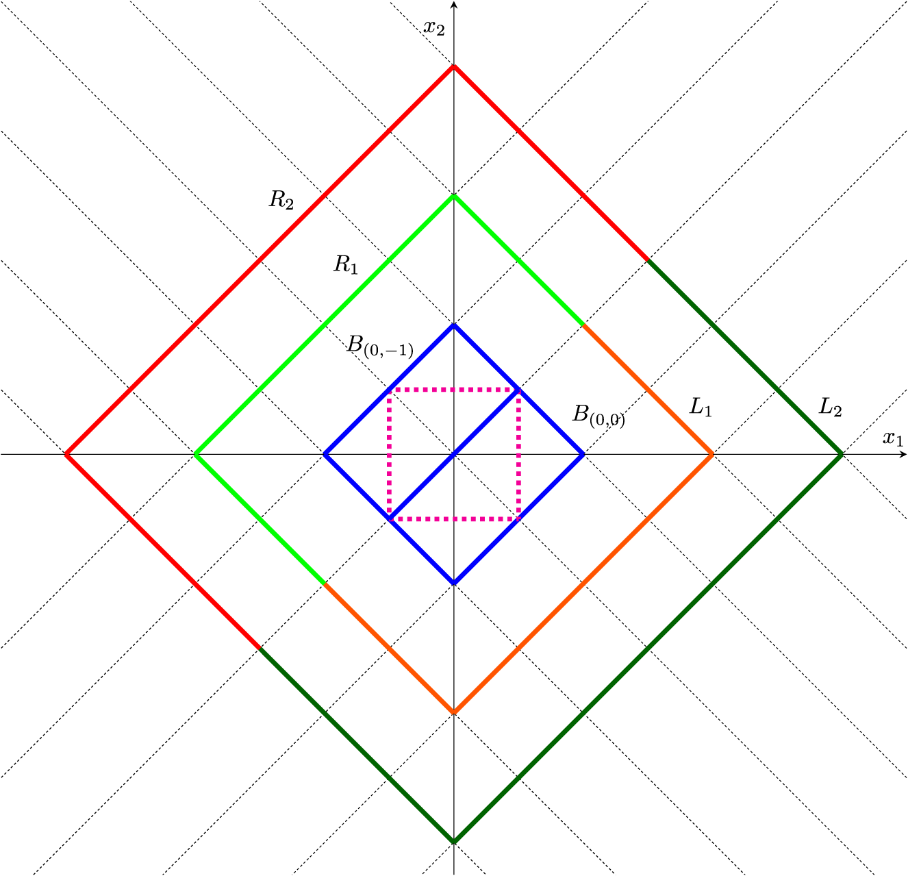
Figure 3 The $x_1x_2$
plane. The initial square we used to define our Zorich map is shown in dashed pink. The rectangle beams
$x_1x_2$
plane. The initial square we used to define our Zorich map is shown in dashed pink. The rectangle beams $B_{(0,0)}$
and
$B_{(0,0)}$
and $B_{(0,-1)}$
are shown in blue, while the sets
$B_{(0,-1)}$
are shown in blue, while the sets $L_1$
,
$L_1$
, $L_2$
,
$L_2$
, $R_1$
and
$R_1$
and $R_2$
are shown in orange, dark green, green and red, respectively.
$R_2$
are shown in orange, dark green, green and red, respectively.
We will show that the space between $S_n$
and
$S_n$
and $S_{n+1}$
(and similarly, between
$S_{n+1}$
(and similarly, between $K_n$
and
$K_n$
and $K_{n+1}$
) is of finite volume and is decreasing as n increases.
$K_{n+1}$
) is of finite volume and is decreasing as n increases.
Lemma 7 Let $I_n$
be the volume that the surface
$I_n$
be the volume that the surface $S_n$
encloses together with the plane
$S_n$
encloses together with the plane $x_3=0$
and inside the beam
$x_3=0$
and inside the beam $B_{(0,0)}$
. Then
$B_{(0,0)}$
. Then $I_n$
is finite for all
$I_n$
is finite for all $n\in \mathbb {N}$
. Furthermore, if
$n\in \mathbb {N}$
. Furthermore, if $T_n:=I_{n+1}-I_n$
is the volume between
$T_n:=I_{n+1}-I_n$
is the volume between $S_n$
and
$S_n$
and $S_{n+1}$
then
$S_{n+1}$
then $T_n$
is a decreasing sequence.
$T_n$
is a decreasing sequence.
Proof. Let us first find an implicit equation that describes each of these surfaces. We work on $B_{(0,0)}$
, but the same can be done on all other rectangle beams. Let us split
$B_{(0,0)}$
, but the same can be done on all other rectangle beams. Let us split $B_{(0,0)}$
into three different beams whose cross-sections with the
$B_{(0,0)}$
into three different beams whose cross-sections with the $x_1x_2$
plane are the sets
$x_1x_2$
plane are the sets
 $$ \begin{align*}Q_1:=h^{-1}(\{(x_1,x_2,x_3)\in S(0,\lambda):0\leq x_2\leq x_1\}),\end{align*} $$
 $$ \begin{align*}\kern9pt Q_2:=h^{-1}(\{(x_1,x_2,x_3)\in S(0,\lambda): x_2\leq 0, x_1\geq 0\})\end{align*} $$
and
 $$ \begin{align*}Q_3:=h^{-1}(\{(x_1,x_2,x_3)\in S(0,\lambda):x_2\leq x_1\leq 0\}),\end{align*} $$
where $S(0,\lambda )$
the sphere of centre
$S(0,\lambda )$
the sphere of centre $0$
and radius
$0$
and radius $\lambda $
. In the beam corresponding to the first cross-section, meaning
$\lambda $
. In the beam corresponding to the first cross-section, meaning $Q_1\times \mathbb {R}$
, the points on the surface
$Q_1\times \mathbb {R}$
, the points on the surface $S_n$
satisfy
$S_n$
satisfy
 $$ \begin{align*}\nu e^{x_3}h_1(x_1,x_2)=-\nu e^{x_3}h_2(x_1,x_2)+2(n+1)\lambda.\end{align*} $$
On the beam $Q_2\times \mathbb {R}$
the surface points satisfy
$Q_2\times \mathbb {R}$
the surface points satisfy
 $$ \begin{align*}\nu e^{x_3}h_1(x_1,x_2)=\nu e^{x_3}h_2(x_1,x_2)+2(n+1)\lambda,\end{align*} $$
while on the beam $Q_3\times \mathbb {R}$
that corresponds to the last cross-section the points satisfy
$Q_3\times \mathbb {R}$
that corresponds to the last cross-section the points satisfy
 $$ \begin{align*}\nu e^{x_3}h_1(x_1,x_2)=-\nu e^{x_3}h_2(x_1,x_2)-2(n+1)\lambda.\end{align*} $$
Suppose now that the surfaces $S_n$
do not intersect the plane
$S_n$
do not intersect the plane $x_3=0$
. Hence the volume that the surface
$x_3=0$
. Hence the volume that the surface $S_n$
encloses together with the plane
$S_n$
encloses together with the plane $x_3=0$
and inside the beam
$x_3=0$
and inside the beam $B_{(0,0)}$
is given by the integrals
$B_{(0,0)}$
is given by the integrals
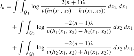 $$ \begin{align*} I_n&=\int\int_{Q_1}\log \frac{2(n+1)\lambda}{\nu(h_2(x_1,x_2)+h_1(x_1,x_2))}\,dx_2\,dx_1\\[6pt] &\quad+\int\int_{Q_2}\log \frac{-2(n+1)\lambda}{\nu(h_1(x_1,x_2)-h_2(x_1,x_2))}\,dx_2\,dx_1\\[6pt] &\quad+\int\int_{Q_3}\log \frac{-2(n+1)\lambda}{\nu(h_2(x_1,x_2)+h_1(x_1,x_2))}\,dx_2\,dx_1. \end{align*} $$
It is not so hard to prove now that each of these integrals is finite since each is an integral of a bounded function except at a neighbourhood of $(0,0)$
and the points where
$(0,0)$
and the points where $h_1\pm h_2 =0$
which are
$h_1\pm h_2 =0$
which are $(0,-2\lambda )$
,
$(0,-2\lambda )$
, $(2\lambda ,0)$
. So in order to show that this sum is finite, it is enough to consider the integrals only in neighbourhoods of those points. On the other hand, when those surfaces
$(2\lambda ,0)$
. So in order to show that this sum is finite, it is enough to consider the integrals only in neighbourhoods of those points. On the other hand, when those surfaces $S_n$
intersect the plane
$S_n$
intersect the plane $x_3=0$
the volumes are no longer given by the above integrals (the set where we integrate will change), but again we only have to consider them at a neighbourhood of
$x_3=0$
the volumes are no longer given by the above integrals (the set where we integrate will change), but again we only have to consider them at a neighbourhood of $(0,0)$
as well as
$(0,0)$
as well as $(0,-2\lambda )$
,
$(0,-2\lambda )$
, $(2\lambda ,0)$
, so that is what we do next. In fact, those volumes in that case are even smaller.
$(2\lambda ,0)$
, so that is what we do next. In fact, those volumes in that case are even smaller.
We will only treat here the second integral around an $\varepsilon $
-neighbourhood of
$\varepsilon $
-neighbourhood of $(0,0)$
, and the rest follows similarly. So we are looking at the integral
$(0,0)$
, and the rest follows similarly. So we are looking at the integral
 $$ \begin{align*}\int\int_{Q_2\cap B(0,\varepsilon)}\log \frac{-2(n+1)\lambda}{\nu(h_2(x_1,x_2)-h_1(x_1,x_2))}\,dx_2\,dx_1,\end{align*} $$
where $B(0,\varepsilon )$
is a ball centred at
$B(0,\varepsilon )$
is a ball centred at $0$
with radius
$0$
with radius $\varepsilon $
. Equivalently, we want to show that the integral
$\varepsilon $
. Equivalently, we want to show that the integral
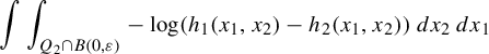 $$ \begin{align}\int\int_{Q_2\cap B(0,\varepsilon)}-\log (h_1(x_1,x_2)-h_2(x_1,x_2))\,dx_2\,dx_1\end{align} $$
is finite. Now because h is a bi-Lipschitz map and because $h_2(x_1,x_2)\leq 0$
and
$h_2(x_1,x_2)\leq 0$
and $h_1(x_1,x_2)\geq 0$
in the set we are integrating we have that
$h_1(x_1,x_2)\geq 0$
in the set we are integrating we have that
 $$ \begin{align*}(h_1-h_2)^2&=h_1^2+h_2^2+2h_1(-h_2)\geq h_1^2+h_2^2\\ &=\sin^2 \theta (h_1^2+h_2^2+(h_3-\lambda)^2)\geq \frac{c_{\varepsilon}}{L^2}(x_1^2+x_2^2),\end{align*} $$
where $\theta $
is the angle between the
$\theta $
is the angle between the $x_3$
-axis and the segment that connects
$x_3$
-axis and the segment that connects $(0,0,\lambda )$
with
$(0,0,\lambda )$
with $(h_1,h_2,h_3)$
, and
$(h_1,h_2,h_3)$
, and $c_{\varepsilon }>0$
is a constant that depends only on
$c_{\varepsilon }>0$
is a constant that depends only on $\varepsilon $
. Hence
$\varepsilon $
. Hence
 $$ \begin{align*}|h_1(x_1,x_2)-h_2(x_1,x_2)|\geq \frac{\sqrt{c_\varepsilon}}{L}\sqrt{x_1^2+x_2^2}.\end{align*} $$
Now since $h_1-h_2\geq 0$
in the set we are integrating, we will have that
$h_1-h_2\geq 0$
in the set we are integrating, we will have that
 $$ \begin{align*}&\int\int_{Q_2\cap B(0,\varepsilon)}\log (h_1(x_1,x_2)-h_2(x_1,x_2))\,dx_2\,dx_1\\ &\quad\geq \int\int_{Q_2\cap B(0,\varepsilon)}\log \bigg(\frac{\sqrt{c_\varepsilon}}{L}\sqrt{x_1^2+x_2^2}\bigg)\,dx_2\,dx_1.\end{align*} $$
Now since the last integral is finite we will have that the integral (4.9) is also finite.
Finally, let us show that the sequence $T_n$
is a decreasing one. Indeed,
$T_n$
is a decreasing one. Indeed,
 $$ \begin{align*}T_n=I_{n+1}-I_n=\lambda^2\log\frac{n+2}{n+1}+\lambda^2 \log\frac{n+2}{n+1}+2\lambda^2\log\frac{n+2}{n+1}=4\lambda^2\log\frac{n+2}{n+1},\end{align*} $$
which can be easily seen to be a decreasing sequence.
Lemma 8 Assume $\lambda>L^{5}$
and let V be a connected subset of
$\lambda>L^{5}$
and let V be a connected subset of $\mathbb {R}^3$
with
$\mathbb {R}^3$
with $m(V)>0$
and such that
$m(V)>0$
and such that $\mathcal {Z}_{\nu }^n(V)$
does not intersect any of the planes
$\mathcal {Z}_{\nu }^n(V)$
does not intersect any of the planes $x_1=\pm x_2 +2\lambda k$
, where
$x_1=\pm x_2 +2\lambda k$
, where $k\in \mathbb {Z}$
for all
$k\in \mathbb {Z}$
for all $n\in \mathbb {N}$
. Then
$n\in \mathbb {N}$
. Then $\mathcal {Z}_{\nu }^n(V)$
visits infinitely often one of the two rectangle beams
$\mathcal {Z}_{\nu }^n(V)$
visits infinitely often one of the two rectangle beams $B_{(0,0)}$
,
$B_{(0,0)}$
, $B_{(0,-1)}$
that have the
$B_{(0,-1)}$
that have the $x_3$
-axis in their boundary.
$x_3$
-axis in their boundary.
Proof. Consider the iterates $V_i=\mathcal {Z}_{\nu }^i(V)$
of the set V. The sets
$V_i=\mathcal {Z}_{\nu }^i(V)$
of the set V. The sets $V_i$
always stay inside one of the rectangle beams by assumption and also they cannot intersect any of the surfaces in
$V_i$
always stay inside one of the rectangle beams by assumption and also they cannot intersect any of the surfaces in $\mathcal {S}$
that are in those beams since if they did on the next iterate they would intersect the boundary of one of the beams. Suppose now that we can find an
$\mathcal {S}$
that are in those beams since if they did on the next iterate they would intersect the boundary of one of the beams. Suppose now that we can find an $N\in \mathbb {N}$
such that
$N\in \mathbb {N}$
such that $V_{i}\not \in B_{(0,0)}\cup B_{(0,-1)}$
for all
$V_{i}\not \in B_{(0,0)}\cup B_{(0,-1)}$
for all $i>N$
. Then by Lemma 6 we have that
$i>N$
. Then by Lemma 6 we have that $m(V_{i})\to \infty $
. This implies that our sets
$m(V_{i})\to \infty $
. This implies that our sets $V_{i}$
cannot lie between any two of the surfaces in
$V_{i}$
cannot lie between any two of the surfaces in $\mathcal {S}$
, for all large i since there is finite volume between them. Thus
$\mathcal {S}$
, for all large i since there is finite volume between them. Thus $V_{i}$
stays below the lowest surface in the relevant rectangle beam for all
$V_{i}$
stays below the lowest surface in the relevant rectangle beam for all $i>N_1>N$
, where
$i>N_1>N$
, where $N_1\in \mathbb {N}$
. This is a contradiction since being below that surface implies that
$N_1\in \mathbb {N}$
. This is a contradiction since being below that surface implies that $V_{i+1}$
is in either
$V_{i+1}$
is in either $B_{(0,0)}$
or
$B_{(0,0)}$
or $B_{(0,-1)}$
.
$B_{(0,-1)}$
.
The next lemma tells us that when a set remains in $B_{(0,0)}$
under iteration by
$B_{(0,0)}$
under iteration by $\mathcal {Z}_{\nu }$
, we can find points with large
$\mathcal {Z}_{\nu }$
, we can find points with large $x_3$
coordinate in its iterates.
$x_3$
coordinate in its iterates.
Lemma 9 Assume $\lambda>L^{5}$
,
$\lambda>L^{5}$
, $\nu>{1}/{\lambda e}$
and let V be a connected set of
$\nu>{1}/{\lambda e}$
and let V be a connected set of $\mathbb {R}^3$
with
$\mathbb {R}^3$
with $m(V)>0$
and such that
$m(V)>0$
and such that $\mathcal {Z}_{\nu }^n(V)$
does not intersect any of the planes
$\mathcal {Z}_{\nu }^n(V)$
does not intersect any of the planes $x_1=\pm x_2 +2\lambda k$
, where
$x_1=\pm x_2 +2\lambda k$
, where $k\in \mathbb {Z}$
for all
$k\in \mathbb {Z}$
for all $n\in \mathbb {N}$
. Suppose that there is an
$n\in \mathbb {N}$
. Suppose that there is an $N_0\in \mathbb {N}$
such that
$N_0\in \mathbb {N}$
such that $\mathcal {Z}_{\nu }^n(V)\subset B_{(0,0)}$
, for all
$\mathcal {Z}_{\nu }^n(V)\subset B_{(0,0)}$
, for all $n>N_0$
. Then, for all
$n>N_0$
. Then, for all $M>0$
and
$M>0$
and $\varepsilon>0$
, there is some
$\varepsilon>0$
, there is some $n_0>N_0$
and a point
$n_0>N_0$
and a point $x\in \mathcal {Z}_{\nu }^{n_0}(V)$
such that
$x\in \mathcal {Z}_{\nu }^{n_0}(V)$
such that $p_3(x)>M$
and
$p_3(x)>M$
and $d(x,x_3\text {-axis})<\varepsilon $
, where d is the euclidean distance.
$d(x,x_3\text {-axis})<\varepsilon $
, where d is the euclidean distance.
Proof. Either an $\varepsilon _0>0$
exists such that
$\varepsilon _0>0$
exists such that $d(\mathcal {Z}_{\nu }^n(V),x_3\text {-axis})>\varepsilon _0$
for all
$d(\mathcal {Z}_{\nu }^n(V),x_3\text {-axis})>\varepsilon _0$
for all $n>N_0$
or such an
$n>N_0$
or such an $\varepsilon _0$
does not exist. In the first case we know from Lemma 6 that
$\varepsilon _0$
does not exist. In the first case we know from Lemma 6 that $m(\mathcal {Z}_{\nu }^n(V))\to \infty $
. We also know that since
$m(\mathcal {Z}_{\nu }^n(V))\to \infty $
. We also know that since $\mathcal {Z}_{\nu }^n(V)\in B_{(0,0)}$
, for all
$\mathcal {Z}_{\nu }^n(V)\in B_{(0,0)}$
, for all $n>N_0$
,
$n>N_0$
, $\mathcal {Z}_{\nu }^n(V)$
must, by Lemma 7, lie below the surface
$\mathcal {Z}_{\nu }^n(V)$
must, by Lemma 7, lie below the surface $S_0$
. Since
$S_0$
. Since $m(\mathcal {Z}_{\nu }^n(V))\to \infty $
, it must be true that for all
$m(\mathcal {Z}_{\nu }^n(V))\to \infty $
, it must be true that for all $M_1>0$
there exist a
$M_1>0$
there exist a $n_0$
and a point
$n_0$
and a point $z_0$
in
$z_0$
in $\mathcal {Z}_{\nu }^{n_0}(V)$
with
$\mathcal {Z}_{\nu }^{n_0}(V)$
with $p_3(z_0)<-M_1$
. The pre-image of that point inside
$p_3(z_0)<-M_1$
. The pre-image of that point inside $B_{(0,0)}$
is a point
$B_{(0,0)}$
is a point $z^{(1)}=(z_1^{(1)},z_2^{(1)},z_3^{(1)})$
for which
$z^{(1)}=(z_1^{(1)},z_2^{(1)},z_3^{(1)})$
for which $\nu e^{z_3^{(1)}}h_3(z_1^{(1)},z_2^{(1)})<-M_1$
and
$\nu e^{z_3^{(1)}}h_3(z_1^{(1)},z_2^{(1)})<-M_1$
and $h_3(z_1^{(1)},z_2^{(1)})<0$
. But since
$h_3(z_1^{(1)},z_2^{(1)})<0$
. But since $h_3>-\lambda $
we have that
$h_3>-\lambda $
we have that
 $$ \begin{align*}e^{z_3^{(1)}}>\frac{M_1}{\nu \lambda}\Rightarrow z_3^{(1)}>\log\frac{ M_1}{\nu \lambda}.\end{align*} $$
If we now take the pre-image in $B_{(0,0)}$
of that point,
$B_{(0,0)}$
of that point, $z^{(2)}=(z_1^{(2)},z_2^{(2)},z_3^{(2)})$
then
$z^{(2)}=(z_1^{(2)},z_2^{(2)},z_3^{(2)})$
then $0<h_3(z_1^{(2)},z_2^{(2)})<\lambda $
and
$0<h_3(z_1^{(2)},z_2^{(2)})<\lambda $
and
 $$ \begin{align*} \nu e^{z_3^{(2)}}h_3(z_1^{(2)},z_2^{(2)})=z_3^{(1)}>\log \frac{M_1}{\nu\lambda},\end{align*} $$
which implies that
 $$ \begin{align*}z_3^{(2)}>\log\frac{\log ({M_1}/{\nu\lambda})}{\nu\lambda}.\end{align*} $$
Thus we have shown that for any $M>0$
there is a point
$M>0$
there is a point $z^{(2)}$
in
$z^{(2)}$
in $\mathcal {Z}_{\nu }^{n_0-2}(V)$
for which
$\mathcal {Z}_{\nu }^{n_0-2}(V)$
for which $z_3^{(2)}>M$
and also
$z_3^{(2)}>M$
and also $|z_1^{(2)}|,|z_2^{(2)}|< \lambda $
. This leads to a contradiction. To see why, note that by our assumptions
$|z_1^{(2)}|,|z_2^{(2)}|< \lambda $
. This leads to a contradiction. To see why, note that by our assumptions $\mathcal {Z}_{\nu }^n(V)$
is
$\mathcal {Z}_{\nu }^n(V)$
is $\varepsilon _0$
away from the
$\varepsilon _0$
away from the $x_3$
-axis and below the surface
$x_3$
-axis and below the surface $S_0$
and thus all of its points, which are also inside the initial square beam
$S_0$
and thus all of its points, which are also inside the initial square beam $[-\lambda ,\lambda ]^2\times \mathbb {R}$
(pink in Figure 3), have a bounded
$[-\lambda ,\lambda ]^2\times \mathbb {R}$
(pink in Figure 3), have a bounded $x_3$
-coordinate. This is true because the surface
$x_3$
-coordinate. This is true because the surface $S_0$
together with any cylinder around the
$S_0$
together with any cylinder around the $x_3$
-axis and the plane
$x_3$
-axis and the plane $x_3=0$
enclose a set inside
$x_3=0$
enclose a set inside $[-\lambda ,\lambda ]^2\times \mathbb {R}$
and outside the cylinder whose closure is compact.
$[-\lambda ,\lambda ]^2\times \mathbb {R}$
and outside the cylinder whose closure is compact.
For the second case, where such an $\varepsilon _0$
does not exist, there is a sequence
$\varepsilon _0$
does not exist, there is a sequence $w_k\in \bigcup _{n>N_0}\mathcal {Z}_{\nu }^n(V)$
with
$w_k\in \bigcup _{n>N_0}\mathcal {Z}_{\nu }^n(V)$
with $d(w_k,x_3\text {-axis})\to 0$
. If
$d(w_k,x_3\text {-axis})\to 0$
. If $p_3(w_k)\to \infty $
we are done. If, on the other hand,
$p_3(w_k)\to \infty $
we are done. If, on the other hand, $p_3(w_k)\to -\infty $
then
$p_3(w_k)\to -\infty $
then $y_k:=\mathcal {Z}_{\nu }(w_k)\to (0,0,0)$
and thus
$y_k:=\mathcal {Z}_{\nu }(w_k)\to (0,0,0)$
and thus $\mathcal {Z}_{\nu }^n(y_k)\to \mathcal {Z}_{\nu }^n(0)=(0,0, E_{\nu \lambda }^n(0))$
, where
$\mathcal {Z}_{\nu }^n(y_k)\to \mathcal {Z}_{\nu }^n(0)=(0,0, E_{\nu \lambda }^n(0))$
, where $E_{\nu \lambda }^n(0))$
converges to
$E_{\nu \lambda }^n(0))$
converges to $\infty $
and again we are done. The remaining case to consider is when there is a subsequence
$\infty $
and again we are done. The remaining case to consider is when there is a subsequence $w_{k_i}$
converging to some point
$w_{k_i}$
converging to some point $(0,0,a)$
in the
$(0,0,a)$
in the $x_3$
-axis. By relabelling we may assume that
$x_3$
-axis. By relabelling we may assume that $w_k\to (0,0,a)$
. Now choose an
$w_k\to (0,0,a)$
. Now choose an $N>0$
such that
$N>0$
such that $E_{\nu \lambda }^N(a)>M$
, where
$E_{\nu \lambda }^N(a)>M$
, where $E_{\nu \lambda }$
denotes the map
$E_{\nu \lambda }$
denotes the map $x\mapsto \nu \lambda e^x$
. By continuity of
$x\mapsto \nu \lambda e^x$
. By continuity of $\mathcal {Z}_{\nu }^N$
, for all
$\mathcal {Z}_{\nu }^N$
, for all $\varepsilon>0$
we may find a
$\varepsilon>0$
we may find a $\delta $
such that if
$\delta $
such that if $|w_k-(0,0,a)|\leq \delta $
, then
$|w_k-(0,0,a)|\leq \delta $
, then
 $$ \begin{align*}|\mathcal{Z}_{\nu}^N(w_k)-\mathcal{Z}_{\nu}^N(0,0,a)|=|\mathcal{Z}^N_{\nu}(w_k)-(0,0,E_{\nu\lambda}^N(a))|\leq \varepsilon.\end{align*} $$
Hence, if we choose $\varepsilon $
small enough we get that
$\varepsilon $
small enough we get that $x_3(\mathcal {Z}^N_{\nu }(w_k))>M$
and
$x_3(\mathcal {Z}^N_{\nu }(w_k))>M$
and $ \mathcal {Z}^N_{\nu }(w_k)$
is within
$ \mathcal {Z}^N_{\nu }(w_k)$
is within $\varepsilon $
distance from the z-axis, when k is large enough.
$\varepsilon $
distance from the z-axis, when k is large enough.
Lemma 10 Let $y_1,y_2\in B(0,r)$
, where
$y_1,y_2\in B(0,r)$
, where $r>0$
. Then for all
$r>0$
. Then for all $n\in \mathbb {N}$
it is true that
$n\in \mathbb {N}$
it is true that
 $$ \begin{align*}|\mathcal{Z}_{\nu}^n(y_1)-\mathcal{Z}_{\nu}^n(y_2)|\leq \bigg(\frac{\max\{L,\lambda\}}{\lambda}\bigg)^n E_{\nu\lambda}(r)\cdots E_{\nu\lambda}^n(r)|y_1-y_2|,\end{align*} $$
where $E_{\nu \lambda }$
denotes the exponential map
$E_{\nu \lambda }$
denotes the exponential map $x\mapsto \nu \lambda e^x$
and L is the bi-Lipschitz constant we used in the construction of the Zorich maps.
$x\mapsto \nu \lambda e^x$
and L is the bi-Lipschitz constant we used in the construction of the Zorich maps.
Proof. The Zorich map is absolutely continuous on any line segment since it is locally Lipschitz. Using the fundamental theorem of calculus for the Lebesgue integral now, it is not too hard to prove that a version of the finite-increment theorem (see [Reference Zorich34, 10.4.1, Theorem 1]) is true for such functions. Specifically, we can prove that
 $$ \begin{align*}|\mathcal{Z}_{\nu}^n(y_1)-\mathcal{Z}_{\nu}^n(y_2)|\leq \operatorname*{\mbox{ess sup}}_{x\in \gamma}|D\mathcal{Z}_{\nu}^n(x)||y_1-y_2|,\end{align*} $$
where $\gamma $
is the line segment that connects
$\gamma $
is the line segment that connects $y_1$
to
$y_1$
to $y_2$
. Remember that
$y_2$
. Remember that $|Df|$
denotes the operator norm of the total derivative. Hence, by the chain rule and elementary properties of linear maps we have that
$|Df|$
denotes the operator norm of the total derivative. Hence, by the chain rule and elementary properties of linear maps we have that
 $$ \begin{align*}|D\mathcal{Z}_{\nu}^n(x)|\leq |D\mathcal{Z}_{\nu}(\mathcal{Z}_{\nu}^{n-1}(x))|\cdots |D\mathcal{Z}_{\nu}(x)|.\end{align*} $$
Hence by the above inequalities and because $y_1,y_2 \in B(0,r)$
we have that
$y_1,y_2 \in B(0,r)$
we have that
 $$ \begin{align}|\mathcal{Z}_{\nu}^n(y_1)-\mathcal{Z}_{\nu}^n(y_2)|\leq&\nonumber \operatorname*{\mbox{ess sup}}_{x\in \gamma}|D\mathcal{Z}_{\nu}(\mathcal{Z}_{\nu}^{n-1}(x))|\cdots \operatorname*{\mbox{ess sup}}_{x\in \gamma}|D\mathcal{Z}_{\nu}(x)||y_1-y_2|\\\leq& \operatorname*{\mbox{ess sup}}_{x\in B(0,r)}|D\mathcal{Z}_{\nu}(\mathcal{Z}_{\nu}^{n-1}(x))|\cdots \operatorname*{\mbox{ess sup}}_{x\in B(0,r)}|D\mathcal{Z}_{\nu}(x)||y_1-y_2|.\end{align} $$
We also know that $D\mathcal {Z}_{\nu }(x)= e^{x_3}D\mathcal {Z}_{\nu }(x_1,x_2,0)$
. Moreover, we will prove that
$D\mathcal {Z}_{\nu }(x)= e^{x_3}D\mathcal {Z}_{\nu }(x_1,x_2,0)$
. Moreover, we will prove that
 $$ \begin{align*}|D\mathcal{Z}_{\nu}(x_1,x_2,0)|\leq \nu\max\{L,\lambda\}.\end{align*} $$
Indeed, let $u=(u_1,u_2,u_3)\in \mathbb {R}^3$
. Then
$u=(u_1,u_2,u_3)\in \mathbb {R}^3$
. Then
 $$ \begin{align*}|D\mathcal{Z}_{\nu}(x_1,x_2,0)|^2=\sup_{|u|=1}|D\mathcal{Z}_{\nu}(x_1,x_2,0)(u)|^2= \nu^2\sup_{|u|=1}|u_1A+u_2B+u_3C|^2, \end{align*} $$
where $A,B, C$
are as in the proof of Lemma 4. Remember now that C is orthogonal to A and B, and thus the above equation becomes
$A,B, C$
are as in the proof of Lemma 4. Remember now that C is orthogonal to A and B, and thus the above equation becomes
 $$ \begin{align*} |D\mathcal{Z}_{\nu}(x_1,x_2,0)|^2&=\nu^2\sup_{|u|=1}(|u_1A+u_2B|^2+|u_3C|^2)\\ &=\nu^2\sup_{|u|=1}(|Dh(x)(u_1,u_2)|^2+|u_3|^2|C|^2)\\ &\leq\nu^2\sup_{|u|=1}(L^2|(u_1,u_2)|^2+\lambda^2|u_3|^2)\\ &\leq\nu^2\max\{L^2,\lambda^2\}, \end{align*} $$
where we have used the fact that h is locally bi-Lipschitz.
Hence, $|D\mathcal {Z}_{\nu }(x)|\leq \nu \max \{L,\lambda \}e^{x_3}$
and (4.10) becomes
$|D\mathcal {Z}_{\nu }(x)|\leq \nu \max \{L,\lambda \}e^{x_3}$
and (4.10) becomes
 $$ \begin{align*}|\mathcal{Z}_{\nu}^n(y_1)-\mathcal{Z}_{\nu}^n(y_2)| &\leq \nu^n\max\{L,\lambda\}^n\sup_{x\in B(0,r)}e^{p_3(\mathcal{Z}_{\nu}^{n-1}(x))}\cdots \sup_{x\in B(0,r)}e^{p_3(x)}|y_1-y_2|\\ &=\bigg(\frac{\max\{L,\lambda\}}{\lambda}\bigg)^n E_{\nu\lambda}(r)\cdots E_{\nu\lambda}^n(r)|y_1-y_2|, \end{align*} $$
where we have used the fact that $\nu \lambda \sup _{x\in B(0,r)}e^{p_3(\mathcal {Z}_{\nu }^{n}(x))}=E_{\nu \lambda }^{n+1}(r)$
which can be easily proved by induction on n.
$\nu \lambda \sup _{x\in B(0,r)}e^{p_3(\mathcal {Z}_{\nu }^{n}(x))}=E_{\nu \lambda }^{n+1}(r)$
which can be easily proved by induction on n.
Proof Proof of Theorem 1
First, let us note that by assumption $\nu>\sqrt {{2L}/{\lambda }}>{1}/{\lambda e}$
. Let V be any open and connected set in
$\nu>\sqrt {{2L}/{\lambda }}>{1}/{\lambda e}$
. Let V be any open and connected set in $\mathbb {R}^3$
. We want to show that
$\mathbb {R}^3$
. We want to show that $\mathcal {Z}_{\nu }^n(V)$
intersects one of the planes that belong to the Julia set for some n and thus V itself intersects the Julia set. Assume that this does not happen. By Lemma 8 we can consider two cases.
$\mathcal {Z}_{\nu }^n(V)$
intersects one of the planes that belong to the Julia set for some n and thus V itself intersects the Julia set. Assume that this does not happen. By Lemma 8 we can consider two cases.
First case. Suppose first that the sequence of iterates $\mathcal {Z}_{\nu }^n(V)$
does not eventually stay inside the square beam
$\mathcal {Z}_{\nu }^n(V)$
does not eventually stay inside the square beam $B_{(0,0)}\cup B_{(0,-1)}$
but also visits their complement infinitely often. Then we can find a subsequence
$B_{(0,0)}\cup B_{(0,-1)}$
but also visits their complement infinitely often. Then we can find a subsequence $n_j$
such that
$n_j$
such that $\mathcal {Z}_{\nu }^{n_j}(V)\in B_{(0,0)}\cup B_{(0,-1)}$
and
$\mathcal {Z}_{\nu }^{n_j}(V)\in B_{(0,0)}\cup B_{(0,-1)}$
and $\mathcal {Z}_{\nu }^{n_j+1}(V)\in B_{(k,l)}$
for some
$\mathcal {Z}_{\nu }^{n_j+1}(V)\in B_{(k,l)}$
for some $(k,l)\not =(0,0),(0,-1)$
. Without loss of generality we may assume that
$(k,l)\not =(0,0),(0,-1)$
. Without loss of generality we may assume that $\mathcal {Z}_{\nu }^{n_j}(V)\in B_{(0,0)}$
.
$\mathcal {Z}_{\nu }^{n_j}(V)\in B_{(0,0)}$
.
Consider now the sets
 $$ \begin{align*}V_{n_j}^+=\bigg\{x\in V: |(p\circ \mathcal{Z}_{\nu}^{n_j})(x)|\geq \frac{\lambda}{2}\bigg\}\end{align*} $$
and
 $$ \begin{align*}V_{n_j}^-=\bigg\{x\in V: |(p\circ \mathcal{Z}_{\nu}^{n_j})(x)|<\frac{\lambda}{2}\bigg\}\end{align*} $$
( $\lambda $
is the scale factor by which we scaled up the initial square). Notice that
$\lambda $
is the scale factor by which we scaled up the initial square). Notice that $V=V_{n_j}^+\cup V_{n_j}^-$
. Since
$V=V_{n_j}^+\cup V_{n_j}^-$
. Since $\mathcal {Z}_{\nu }^{n_j+1}(V)$
is outside of
$\mathcal {Z}_{\nu }^{n_j+1}(V)$
is outside of $B_{(0,0)}\cup B_{(0,-1)}$
we will have that
$B_{(0,0)}\cup B_{(0,-1)}$
we will have that $\mathcal {Z}_{\nu }^{n_j}(V)$
lies between two ‘level surfaces’
$\mathcal {Z}_{\nu }^{n_j}(V)$
lies between two ‘level surfaces’ $S_k$
and
$S_k$
and $S_{k+1}$
, but we know, from Lemma 7, that those surfaces enclose a volume no greater than
$S_{k+1}$
, but we know, from Lemma 7, that those surfaces enclose a volume no greater than $M_0$
between them, where
$M_0$
between them, where $M_0$
is a constant. Thus
$M_0$
is a constant. Thus $m(\mathcal {Z}_{\nu }^{n_j}(V))\leq M_0$
, where m denotes the Lebesgue measure. Also, by Lemma 4, it is true that, for almost all points in
$m(\mathcal {Z}_{\nu }^{n_j}(V))\leq M_0$
, where m denotes the Lebesgue measure. Also, by Lemma 4, it is true that, for almost all points in $V_{n_j}^+$
,
$V_{n_j}^+$
,
 $$ \begin{align*}\det(D\mathcal{Z}_{\nu}^{n_j})\geq{\bigg(\frac{\lambda }{L^5}\bigg)}^{n_j}\frac{1}{\lambda^{3}}|(p\circ \mathcal{Z}_{\nu}^{n_j})(x)|^3\geq{\bigg(\frac{\lambda }{L^5}\bigg)}^{n_j}\frac{1}{8}. \end{align*} $$
Hence, because $\mathcal {Z}_{\nu }^{n_j}$
is a homeomorphism in V we have that
$\mathcal {Z}_{\nu }^{n_j}$
is a homeomorphism in V we have that
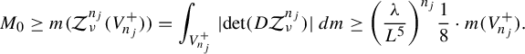 $$ \begin{align*}M_0\geq m(\mathcal{Z}_{\nu}^{n_j}(V_{n_j}^+))=\int_{V_{n_j}^+} |\!\det(D\mathcal{Z}_{\nu}^{n_j})|\,dm\geq{\bigg(\frac{\lambda }{L^5}\bigg)}^{n_j}\frac{1}{8}\cdot m(V_{n_j}^+).\end{align*} $$
This implies that $m(V_{n_j}^+)\to 0$
as
$m(V_{n_j}^+)\to 0$
as $n_j\to \infty $
. On the other hand, the set
$n_j\to \infty $
. On the other hand, the set $\mathcal {Z}_{\nu }^{n_j}(V_{n_j}^-)$
is inside the initial square beam
$\mathcal {Z}_{\nu }^{n_j}(V_{n_j}^-)$
is inside the initial square beam $[-\lambda ,\lambda ]^2\times \mathbb {R}$
. Thus
$[-\lambda ,\lambda ]^2\times \mathbb {R}$
. Thus $\mathcal {Z}_{\nu }^{n_j+1}(V_{n_j}^-)$
lies in the half-space
$\mathcal {Z}_{\nu }^{n_j+1}(V_{n_j}^-)$
lies in the half-space $x_3>0$
and outside the square beam
$x_3>0$
and outside the square beam $B_{(0,0)}\cup B_{(0,-1)}$
. This same set also lies between some level surfaces or below all of them. Moreover, as we proved in Lemma 7, the volume enclosed by those successive surfaces and the volume enclosed by the first one and the plane
$B_{(0,0)}\cup B_{(0,-1)}$
. This same set also lies between some level surfaces or below all of them. Moreover, as we proved in Lemma 7, the volume enclosed by those successive surfaces and the volume enclosed by the first one and the plane $x_3=0$
is smaller than some constant
$x_3=0$
is smaller than some constant $M_0$
. Thus
$M_0$
. Thus $m (\mathcal {Z}_{\nu }^{n_j+1}(V_{n_j}^-))\leq M_0$
. By arguing the same way as before now we get that
$m (\mathcal {Z}_{\nu }^{n_j+1}(V_{n_j}^-))\leq M_0$
. By arguing the same way as before now we get that
 $$ \begin{align*}M_0\geq m(\mathcal{Z}_{\nu}^{n_j+1}(V_{n_j}^-))=\int_{V_{n_j}^-} |\!\det(D\mathcal{Z}_{\nu}^{n_j+1})|\,dm\geq{\bigg(\frac{\lambda }{L^5}\bigg)}^{n_j+1}\frac{1}{8}\cdot m(V_{n_j}^-).\end{align*} $$
This again implies that $ m(V_{n_j}^-)\to 0$
as
$ m(V_{n_j}^-)\to 0$
as $n_j\to \infty $
. But this is a contradiction since
$n_j\to \infty $
. But this is a contradiction since $m(V)=m(V_{n_j}^-)+m(V_{n_j}^+)$
.
$m(V)=m(V_{n_j}^-)+m(V_{n_j}^+)$
.
Second case. Suppose now that $\mathcal {Z}_{\nu }^n(V)\in B_{(0,0)}\cup B_{(0,-1)}$
, for all
$\mathcal {Z}_{\nu }^n(V)\in B_{(0,0)}\cup B_{(0,-1)}$
, for all $n>N_0$
. Observe that either
$n>N_0$
. Observe that either $\mathcal {Z}_{\nu }(B_{(0,0)})\subset \{(x_1,x_2,x_3):x_2\leq x_1\}$
or
$\mathcal {Z}_{\nu }(B_{(0,0)})\subset \{(x_1,x_2,x_3):x_2\leq x_1\}$
or $\mathcal {Z}_{\nu }(B_{(0,0)})\subset \{(x_1,x_2,x_3):x_2\geq x_1\}$
. In the first case
$\mathcal {Z}_{\nu }(B_{(0,0)})\subset \{(x_1,x_2,x_3):x_2\geq x_1\}$
. In the first case $\mathcal {Z}_{\nu }^n(V)$
stays in
$\mathcal {Z}_{\nu }^n(V)$
stays in $B_{(0,0)}$
for all large n or it stays in
$B_{(0,0)}$
for all large n or it stays in $B_{(0,-1)}$
, while in the second it alternates between
$B_{(0,-1)}$
, while in the second it alternates between $B_{(0,0)}$
and
$B_{(0,0)}$
and $B_{(0,-1)}$
. For simplicity we will assume that the first case holds and thus
$B_{(0,-1)}$
. For simplicity we will assume that the first case holds and thus $\mathcal {Z}_{\nu }^n(V)\in B_{(0,0)}$
, for all
$\mathcal {Z}_{\nu }^n(V)\in B_{(0,0)}$
, for all $n>N_0$
.
$n>N_0$
.
Let us now consider the inverse image under $\mathcal {Z}_{\nu }$
of the boundary of
$\mathcal {Z}_{\nu }$
of the boundary of $B_{(0,0)}$
, which lies inside
$B_{(0,0)}$
, which lies inside $B_{(0,0)}$
, namely the surface
$B_{(0,0)}$
, namely the surface $S_0$
we had in the proof of Lemma 7. Remember that this surface is defined as
$S_0$
we had in the proof of Lemma 7. Remember that this surface is defined as $S_0:=\{(x_1,x_2,x_3)\in B_{(0,0)}:x_3=f(x_1,x_2)\}$
, where f is continuous on
$S_0:=\{(x_1,x_2,x_3)\in B_{(0,0)}:x_3=f(x_1,x_2)\}$
, where f is continuous on $B_{(0,0)}\cap \{x_3=0\}$
and extends continuously on the boundary of this set except at the points
$B_{(0,0)}\cap \{x_3=0\}$
and extends continuously on the boundary of this set except at the points $(0,0)$
,
$(0,0)$
, $(2\lambda ,0)$
,
$(2\lambda ,0)$
, $(0,-2\lambda )$
where
$(0,-2\lambda )$
where $f\to \infty $
. Notice then that all the iterates
$f\to \infty $
. Notice then that all the iterates $\mathcal {Z}_{\nu }^n(V)$
stay below the surface
$\mathcal {Z}_{\nu }^n(V)$
stay below the surface $S_0$
.
$S_0$
.
Consider now a plane $x_3=c$
, with
$x_3=c$
, with $c=E^{N}_{\nu \lambda }(0)-\lambda $
and N so large that this plane intersects this surface
$c=E^{N}_{\nu \lambda }(0)-\lambda $
and N so large that this plane intersects this surface $S_0$
and also
$S_0$
and also
 $$ \begin{align} (c+\lambda)^{\log (c+\lambda)+1}e^{c+\lambda}\nu^2\lambda^2 e^{-({\nu\lambda e^c}/{2})}\leq \lambda. \end{align} $$
We define sets $A_1$
,
$A_1$
, $A_2$
and
$A_2$
and $A_3$
as follows:
$A_3$
as follows:
-
•
$A_1:=\{(x_1,x_2,x_3)\in B_{(0,0)}:c<x_3<f(x_1,x_2)\ \text {and}\ (x_1,x_2)\ \text {in a neighbourhood of} (0,0)\}$
; -
•
$A_2:=\{(x_1,x_2,x_3)\in B_{(0,0)}:c<x_3<f(x_1,x_2)\ \text {and}\ (x_1,x_2)\ \text {in a neighbourhood of} (2\lambda ,0)\}$
; -
•
$A_3:=\{(x_1,x_2,x_3)\in B_{(0,0)}:c<x_3<f(x_1,x_2)\ \text {and}\ (x_1,x_2)\ \text {in a neighbourhood of} (0,-2\lambda )\}$
.


Then the following assertions hold.
-
(i) All those sets lie below (in terms of the
$x_3$
-coordinate) the surface
$S_0$
. By the definitions and Lemma 7 it is easy to see that the sets
$A_1$
,
$A_2$
and
$A_3$
are also of finite Lebesgue measure. -
(ii)
$\mathcal {Z}_{\nu }(A_2\cup A_3)\subset \{(x_1,x_2,x_3)\in \mathbb {R}^3:x_3< -({\nu \lambda e^c}/{2})\}$
and thus
$\mathcal {Z}^2_{\nu }(A_2\cup A_3)\subset B(0,\delta ), $
where
$\delta = \nu \lambda e^{-({\nu \lambda e^c}/{2})}$
. Note that
$\delta <\nu \lambda =E_{\nu \lambda }(0)$
. -
(iii) It is easy to show by induction on N and since
$\nu \lambda>1/e$
that
$E_{\nu \lambda }^N(0)\geq E_{\nu \lambda }(N-1)$
and thus (4.12)
$$ \begin{align} E_{\nu\lambda}(N-1)\leq c+\lambda\Rightarrow N \leq \log(c+\lambda)+2. \end{align} $$


By Lemma 10 and since $\lambda> L^5$
we will now have that, for all
$\lambda> L^5$
we will now have that, for all $x\in B(0,\delta )$
,
$x\in B(0,\delta )$
,
 $$ \begin{align*}|\mathcal{Z}_{\nu}^N(x)-\mathcal{Z}_{\nu}^N(0)|&\leq E_{\nu\lambda}(\delta)\cdots E_{\nu\lambda}^N(\delta)|x|\\ &\leq E^2_{\nu\lambda}(0)\cdots E_{\nu\lambda}^{N+1}(0)\delta\\ &\leq(c+\lambda)^{N-1}E_{\nu\lambda}(\lambda+c)\delta\\ &\leq(c+\lambda)^{\log(c+\lambda )+1}\nu\lambda e^{\lambda+c}\delta.\end{align*} $$
Hence, by (4.11) we will have that
 $$ \begin{align} |\mathcal{Z}_{\nu}^N(x)-\mathcal{Z}_{\nu}^N(0)|\leq \lambda. \end{align} $$
Equation (4.13) together with (ii) implies that $\mathcal {Z}_{\nu }^{N+2}(A_2\cup A_3)\subset B(\mathcal {Z}_{\nu }^{N}(0),\lambda )$
, and by the choice of c this last ball is contained in
$\mathcal {Z}_{\nu }^{N+2}(A_2\cup A_3)\subset B(\mathcal {Z}_{\nu }^{N}(0),\lambda )$
, and by the choice of c this last ball is contained in $\{(x_1,x_2,x_3)\in \mathbb {R}^3:x_3>c\}$
. This implies that the part of
$\{(x_1,x_2,x_3)\in \mathbb {R}^3:x_3>c\}$
. This implies that the part of $\mathcal {Z}_{\nu }^{N+2}(A_2\cup A_3)$
that lies below
$\mathcal {Z}_{\nu }^{N+2}(A_2\cup A_3)$
that lies below $S_0$
is contained in
$S_0$
is contained in $A_1$
.
$A_1$
.
Recall that $\mathcal {Z}_\nu ^n(V)$
stays below
$\mathcal {Z}_\nu ^n(V)$
stays below $S_0$
for
$S_0$
for $n>N_0$
. By Lemma 9 we know that there is a point
$n>N_0$
. By Lemma 9 we know that there is a point $x_0\in \mathcal {Z}_{\nu }^{n_0}(V)$
for some
$x_0\in \mathcal {Z}_{\nu }^{n_0}(V)$
for some $n_0>N_0$
such that
$n_0>N_0$
such that $x_0\in A_1$
. Take such a point
$x_0\in A_1$
. Take such a point $x_0$
. Let us carefully examine the behaviour of the iterates of this point. We can assume that
$x_0$
. Let us carefully examine the behaviour of the iterates of this point. We can assume that $A_1$
is so close to the
$A_1$
is so close to the $x_3$
-axis that if
$x_3$
-axis that if $y\in A_1$
then
$y\in A_1$
then $p_3(\mathcal {Z}_{\nu }(y))>p_3(y)$
by Lemma 5(a). Hence the points
$p_3(\mathcal {Z}_{\nu }(y))>p_3(y)$
by Lemma 5(a). Hence the points $\mathcal {Z}_{\nu }^n(x_0)$
go higher and higher up in the
$\mathcal {Z}_{\nu }^n(x_0)$
go higher and higher up in the $x_3$
direction, while at the same time staying in
$x_3$
direction, while at the same time staying in $A_1$
, until at some point the iterate
$A_1$
, until at some point the iterate $\mathcal {Z}_{\nu }^k(x_0)$
, for some k, will lie in either
$\mathcal {Z}_{\nu }^k(x_0)$
, for some k, will lie in either $A_2$
or
$A_2$
or $A_3$
thanks to Lemma 5(b). Without loss of generality assume that
$A_3$
thanks to Lemma 5(b). Without loss of generality assume that $x_1:=\mathcal {Z}_{\nu }^{k}(x_0)\in A_2$
and take a small ball around
$x_1:=\mathcal {Z}_{\nu }^{k}(x_0)\in A_2$
and take a small ball around $x_1$
,
$x_1$
, $B(x_1,r)$
with
$B(x_1,r)$
with $B(x_1,r)\subset A_2\cap \mathcal {Z}^{n_0+k}_{\nu }(V)$
. By what we have said in the previous paragraph, we will have that
$B(x_1,r)\subset A_2\cap \mathcal {Z}^{n_0+k}_{\nu }(V)$
. By what we have said in the previous paragraph, we will have that $\mathcal {Z}_{\nu }^{N+2}(B(x_1,r))\subset ~A_1$
.
$\mathcal {Z}_{\nu }^{N+2}(B(x_1,r))\subset ~A_1$
.
However, we know what happens in points inside $A_1$
when we iterate: they eventually leave
$A_1$
when we iterate: they eventually leave $A_1$
. Thus for some
$A_1$
. Thus for some $k>N+2$
we will have that
$k>N+2$
we will have that $\mathcal {Z}_{\nu }^{k}(B(x_1,r))\subset A_2 \cup A_3$
since
$\mathcal {Z}_{\nu }^{k}(B(x_1,r))\subset A_2 \cup A_3$
since $B(x_1,r)$
is a connected set and the sets
$B(x_1,r)$
is a connected set and the sets $A_1$
,
$A_1$
, $A_2$
and
$A_2$
and $A_3$
are disjoint. We can then repeat this whole argument, meaning that we take the set
$A_3$
are disjoint. We can then repeat this whole argument, meaning that we take the set $\mathcal {Z}_{\nu }^{k}(B(x_1,r))$
which is now in
$\mathcal {Z}_{\nu }^{k}(B(x_1,r))$
which is now in $A_2$
or
$A_2$
or $A_3$
and thus will get mapped by
$A_3$
and thus will get mapped by $\mathcal {Z}_{\nu }$
to the lower half-space
$\mathcal {Z}_{\nu }$
to the lower half-space $x_3<-({\nu \lambda e^c}/{2})$
and by
$x_3<-({\nu \lambda e^c}/{2})$
and by $\mathcal {Z}_{\nu }^{N+2}$
inside
$\mathcal {Z}_{\nu }^{N+2}$
inside $A_1$
. Now continue as above and then repeat. Eventually we obtain a sequence
$A_1$
. Now continue as above and then repeat. Eventually we obtain a sequence $n_j\to \infty $
with
$n_j\to \infty $
with
 $$ \begin{align*}\mathcal{Z}_{\nu}^{n_j}(B(x_1,r))\subset A_2 \cup A_3.\end{align*} $$
Then by using Lemma 6 we will have that $m(\mathcal {Z}_{\nu }^{n_j}(B(x_1,r)))\to \infty $
, but this is impossible since
$m(\mathcal {Z}_{\nu }^{n_j}(B(x_1,r)))\to \infty $
, but this is impossible since $m(A_2\cup A_3)$
is finite.
$m(A_2\cup A_3)$
is finite.
5 Escaping set of the Zorich maps
In this section we prove that the escaping set is connected for those Zorich maps for which Theorem 1 holds. Note that we assume that $\lambda>L^5$
and
$\lambda>L^5$
and $\nu>\sqrt {{2L}/{\lambda }}$
.
$\nu>\sqrt {{2L}/{\lambda }}$
.
The proof of this theorem closely follows Rempe’s proof for the connectivity of the escaping set of the exponential family in [Reference Rempe27]. Before we begin with the proof we need to define a few things. First, in this section, for simplicity and without loss of generality we will assume that our Zorich map sends $B_{(0,0)}$
in the half-space
$B_{(0,0)}$
in the half-space $\{(x_1,x_2,x_3)\in \mathbb {R}^3:x_2\leq x_1\}$
. Let
$\{(x_1,x_2,x_3)\in \mathbb {R}^3:x_2\leq x_1\}$
. Let
 $$ \begin{align*}\mathbb{H}_0:=\{(x_1,x_2,x_3)\in\mathbb{R}^3:x_2<x_1\ \text{and}\ x_2>-x_1\},\end{align*} $$
and similarly,
 $$ \begin{align*}\mathbb{H}_1:=\{(x_1,x_2,x_3)\in\mathbb{R}^3:x_2>x_1\ \text{and}\ x_2>-x_1\},\end{align*} $$
 $$ \begin{align*}\mathbb{H}_2:=\{(x_1,x_2,x_3)\in\mathbb{R}^3:x_2>x_1\ \text{and}\ x_2<-x_1\},\end{align*} $$
 $$ \begin{align*}\mathbb{H}_3:=\{(x_1,x_2,x_3)\in\mathbb{R}^3:x_2<x_1\ \text{and}\ x_2<-x_1\}.\end{align*} $$
Also, let $T_0=T_{(0,0)}:=B_{(0,0)}\cap \mathbb {H}_0$
and
$T_0=T_{(0,0)}:=B_{(0,0)}\cap \mathbb {H}_0$
and
 $$ \begin{align*}T_{(i,j)}=T_{(0,0)}+i(\lambda,\lambda,0)+j(\lambda,-\lambda,0),\quad i,j\in\mathbb{Z}.\end{align*} $$
Note that $T_1:=T_{(0,-1)}=B_{(0,-1)}\cap \mathbb {H}_1$
,
$T_1:=T_{(0,-1)}=B_{(0,-1)}\cap \mathbb {H}_1$
, $T_2:=T_{(-1,-1)}=B_{(0,-1)}\cap \mathbb {H}_2$
and
$T_2:=T_{(-1,-1)}=B_{(0,-1)}\cap \mathbb {H}_2$
and $T_3:=T_{(-1,0)}=B_{(0,0)}\cap \mathbb {H}_3$
and thus
$T_3:=T_{(-1,0)}=B_{(0,0)}\cap \mathbb {H}_3$
and thus $T_{i}\subset \mathbb {H}_i$
,
$T_{i}\subset \mathbb {H}_i$
, $i=0,1,2,3$
. Now define
$i=0,1,2,3$
. Now define $\Lambda _i :\mathbb {H}_i\to T_i$
,
$\Lambda _i :\mathbb {H}_i\to T_i$
, $i=0,1,2,3$
, to be the inverse branches of
$i=0,1,2,3$
, to be the inverse branches of $\mathcal {Z}_{\nu }$
in
$\mathcal {Z}_{\nu }$
in $T_i$
. We can extend those maps to
$T_i$
. We can extend those maps to $\overline {\mathbb {H}_i}\setminus \{0\}$
for
$\overline {\mathbb {H}_i}\setminus \{0\}$
for $i=0,1,2,3$
, and again those extended maps are injective. We will use the same symbols
$i=0,1,2,3$
, and again those extended maps are injective. We will use the same symbols $\Lambda _i$
to denote these extended maps.
$\Lambda _i$
to denote these extended maps.
Now take $\gamma _0:=\{(0,0,x_3):x_3<0\}$
and inductively define
$\gamma _0:=\{(0,0,x_3):x_3<0\}$
and inductively define
 $$ \begin{align*}\gamma_{k}:=\Lambda_0(\gamma_{k-1}),\end{align*} $$
for all $k\geq 1$
. Each of the sets
$k\geq 1$
. Each of the sets $\gamma _{k}$
,
$\gamma _{k}$
, $k\geq 1$
, is an injective curve inside
$k\geq 1$
, is an injective curve inside $\overline {T_0}$
.
$\overline {T_0}$
.
We now define the set $\Gamma _0$
by
$\Gamma _0$
by
 $$ \begin{align*}\Gamma_0:=\bigcup_{k\geq0}\gamma_{k}.\end{align*} $$
Lemma 11 If $U\subset \mathbb {R}^3$
is any open set with
$U\subset \mathbb {R}^3$
is any open set with $U\cap \overline {\Gamma _0}\not =\emptyset $
then there is a
$U\cap \overline {\Gamma _0}\not =\emptyset $
then there is a $k_0\in \mathbb {N}$
with
$k_0\in \mathbb {N}$
with $\gamma _k\cap U\not =\emptyset $
for all
$\gamma _k\cap U\not =\emptyset $
for all $k>k_0$
. In particular,
$k>k_0$
. In particular, $\bigcup _{k\geq k_0}\gamma _k$
is dense in
$\bigcup _{k\geq k_0}\gamma _k$
is dense in $\overline {\Gamma _0}$
.
$\overline {\Gamma _0}$
.
Proof. Let $x_0\in \overline {\Gamma _0}$
, and let U be a neighbourhood of this point. We want to show that
$x_0\in \overline {\Gamma _0}$
, and let U be a neighbourhood of this point. We want to show that $\gamma _{k}\cap U\not =\emptyset $
for all sufficiently large k. We know, from the definition of
$\gamma _{k}\cap U\not =\emptyset $
for all sufficiently large k. We know, from the definition of $\overline {\Gamma _0}$
, that there is a point
$\overline {\Gamma _0}$
, that there is a point $x_1\in U\cap \Gamma _0 $
. This implies that
$x_1\in U\cap \Gamma _0 $
. This implies that $\mathcal {Z}_{\nu }^n(x_1)$
belongs to the
$\mathcal {Z}_{\nu }^n(x_1)$
belongs to the $x_3$
-axis for all
$x_3$
-axis for all $n\geq N_0$
, for some
$n\geq N_0$
, for some $N_0\in \mathbb {N}$
, and in fact we can assume that
$N_0\in \mathbb {N}$
, and in fact we can assume that $x_2:=\mathcal {Z}_{\nu }^{N_0}(x_1)\in H_{>M},$
where M is any positive number. Now taking
$x_2:=\mathcal {Z}_{\nu }^{N_0}(x_1)\in H_{>M},$
where M is any positive number. Now taking $M>M_0$
, where
$M>M_0$
, where $M_0$
is the constant we used in Lemma 1, and applying that lemma n times for a ball
$M_0$
is the constant we used in Lemma 1, and applying that lemma n times for a ball $B(x_2,R)\subset \mathcal {Z}_{\nu }^{N_0}(U)$
, we obtain
$B(x_2,R)\subset \mathcal {Z}_{\nu }^{N_0}(U)$
, we obtain
 $$ \begin{align*}\mathcal{Z}_{\nu}^{n}(B(x_2,R)\cap H_{>M})\supset B(\mathcal{Z}^n_{\nu}(x_2),\alpha^{-n}R)\cap H_{>E^n_{\nu\lambda}(M)}.\end{align*} $$
For all large enough n the ball on the right-hand side, $B(\mathcal {Z}^n_{\nu }(x_2),\alpha ^{-n}R)$
, intersects the line
$B(\mathcal {Z}^n_{\nu }(x_2),\alpha ^{-n}R)$
, intersects the line $\gamma _1=\{(2\lambda ,0,t):t\in \mathbb {R}\}$
. Hence, for all large enough n,
$\gamma _1=\{(2\lambda ,0,t):t\in \mathbb {R}\}$
. Hence, for all large enough n, $\mathcal {Z}_{\nu }^n(U)$
intersects
$\mathcal {Z}_{\nu }^n(U)$
intersects $\gamma _1$
. Thus for each n large enough there is a point
$\gamma _1$
. Thus for each n large enough there is a point $x_3\in \gamma _1$
whose backward orbit intersects U itself. This means that U contains a point in
$x_3\in \gamma _1$
whose backward orbit intersects U itself. This means that U contains a point in $\gamma _{k}$
for all large enough k, as we wanted.
$\gamma _{k}$
for all large enough k, as we wanted.
Lemma 12 The set $\Gamma _0$
is connected.
$\Gamma _0$
is connected.
Proof. Suppose $U\subset \mathbb {R}^3$
is an open set with
$U\subset \mathbb {R}^3$
is an open set with $U\cap \Gamma _0\not =\emptyset $
and
$U\cap \Gamma _0\not =\emptyset $
and $\Gamma _0\cap \partial U=\emptyset $
. We show that
$\Gamma _0\cap \partial U=\emptyset $
. We show that $\Gamma _0\subset U$
.
$\Gamma _0\subset U$
.
By Lemma 11 we have that $\gamma _k\cap U\not =\emptyset $
, for all
$\gamma _k\cap U\not =\emptyset $
, for all $k>k_0$
. Since
$k>k_0$
. Since $\gamma _k$
is a connected curve, this implies that
$\gamma _k$
is a connected curve, this implies that $\gamma _k\subset U$
, for all
$\gamma _k\subset U$
, for all $k> k_0$
. Thus
$k> k_0$
. Thus
 $$ \begin{align*}\Gamma_0\subset \overline{\Gamma_0}= \overline{\bigcup_{k\geq k_0}\gamma_k}\subset \overline{U}.\end{align*} $$
Hence, since $\Gamma _0\cap \partial U=\emptyset $
, we have that
$\Gamma _0\cap \partial U=\emptyset $
, we have that $\Gamma _0\subset U$
.
$\Gamma _0\subset U$
.
Similarly, we can define sets $\Gamma _i$
, for
$\Gamma _i$
, for $i=1,2,3$
, using this time
$i=1,2,3$
, using this time $\Lambda _i$
instead of
$\Lambda _i$
instead of $\Lambda _0$
and prove that
$\Lambda _0$
and prove that $\Gamma _i$
is also connected. This implies that the union
$\Gamma _i$
is also connected. This implies that the union $\Gamma :=\bigcup _{i=0}^3\Gamma _i$
is a connected set. Define the set
$\Gamma :=\bigcup _{i=0}^3\Gamma _i$
is a connected set. Define the set
 $$ \begin{align*}Y:=\bigcup_{(k,l)\in\mathbb{Z}^2}(\Gamma+k(2\lambda,2\lambda,0)+l(2\lambda,-2\lambda,0)),\end{align*} $$
which is connected since $\Gamma $
contains the lines
$\Gamma $
contains the lines $\{(\pm 2\lambda ,0,t):t\in \mathbb {R}\}$
,
$\{(\pm 2\lambda ,0,t):t\in \mathbb {R}\}$
, $\{(0,\pm 2\lambda ,t):t\in \mathbb {R}\}$
and is a subset of
$\{(0,\pm 2\lambda ,t):t\in \mathbb {R}\}$
and is a subset of $I(\mathcal {Z}_{\nu })$
since the iterates of any point eventually land on the
$I(\mathcal {Z}_{\nu })$
since the iterates of any point eventually land on the $x_3$
-axis. Next we define, inductively, the sets
$x_3$
-axis. Next we define, inductively, the sets $Y_j\subset I(\mathcal {Z}_{\nu })$
by setting
$Y_j\subset I(\mathcal {Z}_{\nu })$
by setting $Y_0=Y$
and
$Y_0=Y$
and $Y_{j+1}=\mathcal {Z}_{\nu }^{-1}(Y_j)\cup Y_j$
.
$Y_{j+1}=\mathcal {Z}_{\nu }^{-1}(Y_j)\cup Y_j$
.
Lemma 13 The sets $Y_j$
are connected for all
$Y_j$
are connected for all $j\geq 0$
.
$j\geq 0$
.
Proof. We will prove this by induction on j. Let us define the inverse branches of $\mathcal {Z}_{\nu }$
. Using the notation we introduced in the first paragraphs of this section, define
$\mathcal {Z}_{\nu }$
. Using the notation we introduced in the first paragraphs of this section, define $\Lambda _{k,l}:\mathbb {H}_p\to T_{(k,l)}$
, with
$\Lambda _{k,l}:\mathbb {H}_p\to T_{(k,l)}$
, with $p=0,1,2,3$
, to be the inverse branches of
$p=0,1,2,3$
, to be the inverse branches of $\mathcal {Z}_{\nu }$
that take values on the square beams
$\mathcal {Z}_{\nu }$
that take values on the square beams $T_{(k,l)}$
. We also extend those maps to
$T_{(k,l)}$
. We also extend those maps to $\overline {\mathbb {H}_p}\setminus \{0\}$
and use the same symbol to denote those extensions. With that notation we have that
$\overline {\mathbb {H}_p}\setminus \{0\}$
and use the same symbol to denote those extensions. With that notation we have that
 $$ \begin{align*}Y_{j+1}=\bigcup_{(k,l)\in\mathbb{Z}^2}\Lambda_{k,l}(Y_j)\cup Y_j.\end{align*} $$
By the inductive hypothesis now we know that $Y_j$
is connected and because
$Y_j$
is connected and because $\Lambda _{k,l}$
is continuous the set
$\Lambda _{k,l}$
is continuous the set $\Lambda _{k,l}(Y_j)$
is also connected. Observe now that the point
$\Lambda _{k,l}(Y_j)$
is also connected. Observe now that the point $x_{n,m}=(2\lambda ,0,0)+n(2\lambda ,0,0)+m(0,2\lambda ,0)$
is inside
$x_{n,m}=(2\lambda ,0,0)+n(2\lambda ,0,0)+m(0,2\lambda ,0)$
is inside $Y=Y_0$
and thus in
$Y=Y_0$
and thus in $Y_j$
, for all
$Y_j$
, for all $n,m\in \mathbb {Z}$
and for all
$n,m\in \mathbb {Z}$
and for all $j\in \mathbb {N}$
. Also note that
$j\in \mathbb {N}$
. Also note that $\mathcal {Z}_{\nu }(x_{n,m})=(0,0,-\nu \lambda )$
or
$\mathcal {Z}_{\nu }(x_{n,m})=(0,0,-\nu \lambda )$
or $(0,0,\nu \lambda )$
which are both points in
$(0,0,\nu \lambda )$
which are both points in $Y_j$
. This means that there are
$Y_j$
. This means that there are $m, n$
depending on
$m, n$
depending on $k,l$
such that
$k,l$
such that $x_{n,m}\in \Lambda _{k,l}(Y_j)$
. Hence
$x_{n,m}\in \Lambda _{k,l}(Y_j)$
. Hence $\Lambda _{k,l}(Y_j)\cap Y_j\not =\emptyset $
. This implies that the set
$\Lambda _{k,l}(Y_j)\cap Y_j\not =\emptyset $
. This implies that the set $\Lambda _{k,l}(Y_j)\cup Y_j$
is connected. Hence
$\Lambda _{k,l}(Y_j)\cup Y_j$
is connected. Hence $Y_{j+1}$
is connected as a union of connected sets with non-empty intersections with each other, as we wanted.
$Y_{j+1}$
is connected as a union of connected sets with non-empty intersections with each other, as we wanted.
Proof Proof of Theorem 3
Consider the set
 $$ \begin{align*}\bigcup_{j\geq 0}\mathcal{Z}_{\nu}^{-j}((0,0,-1))\subset\bigcup_{j\geq 0}Y_j.\end{align*} $$
The Zorich map is bounded on $\{(x_1,x_2,x_3):x_3<0\}$
and thus it does not have the pits effect (see [Reference Bergweiler and Nicks5]). Hence, by [Reference Bergweiler and Nicks5, Theorem 1.8] we will have that the set
$\{(x_1,x_2,x_3):x_3<0\}$
and thus it does not have the pits effect (see [Reference Bergweiler and Nicks5]). Hence, by [Reference Bergweiler and Nicks5, Theorem 1.8] we will have that the set $\bigcup _{j\geq 0}\mathcal {Z}_{\nu }^{-j}((0,0,-1))$
is dense in
$\bigcup _{j\geq 0}\mathcal {Z}_{\nu }^{-j}((0,0,-1))$
is dense in $\mathcal {J}(\mathcal {Z}_\nu )$
, which by Theorem 1 is
$\mathcal {J}(\mathcal {Z}_\nu )$
, which by Theorem 1 is $\mathbb {R}^3$
, and thus also dense in
$\mathbb {R}^3$
, and thus also dense in $I(\mathcal {Z}_{\nu })$
. Thus the set
$I(\mathcal {Z}_{\nu })$
. Thus the set $\bigcup _{j\geq 0}Y_j $
is a connected dense subset of
$\bigcup _{j\geq 0}Y_j $
is a connected dense subset of $I(\mathcal {Z}_{\nu })$
which implies that the escaping set itself is connected.
$I(\mathcal {Z}_{\nu })$
which implies that the escaping set itself is connected.
6 Density of periodic points
Proof Proof of Theorem 2
First let $U_0=B(x_0,r)$
be a ball centred at
$U_0=B(x_0,r)$
be a ball centred at $x_0\in \mathbb {R}^3$
of radius
$x_0\in \mathbb {R}^3$
of radius $r>0$
. We seek a periodic point of
$r>0$
. We seek a periodic point of $\mathcal {Z}_\nu $
in
$\mathcal {Z}_\nu $
in $U_0$
. Without loss of generality we may assume that
$U_0$
. Without loss of generality we may assume that $\overline {U_0}$
does not intersect any of the planes
$\overline {U_0}$
does not intersect any of the planes $x_1=\pm x_2+2\lambda k$
,
$x_1=\pm x_2+2\lambda k$
, $k\in \mathbb {Z}$
.
$k\in \mathbb {Z}$
.
We will follow the method of [Reference Fletcher and Nicks16] where the authors prove that periodic points of a quasiregular version of the sine function are dense on $\mathbb {R}^3$
. We will do this by finding an
$\mathbb {R}^3$
. We will do this by finding an $N\in \mathbb {N}$
and a finite sequence of open sets
$N\in \mathbb {N}$
and a finite sequence of open sets $U_j$
,
$U_j$
, $j=0,\ldots , N$
, such that:
$j=0,\ldots , N$
, such that:
-
(i)
$U_{j+1}\subset \mathcal {Z}_{\nu }(U_j)$
,
$0\leq j\leq N-1$
; -
(ii)
$\mathcal {Z}_{\nu }$
is a homeomorphism on each
$U_j$
for
$j\leq N-1$
; -
(iii)
$\overline {U_0}\subset U_N$
.


If these conditions are met then we can define a continuous inverse branch $\mathcal {Z}^{-N}_{\nu }:U_N\to U_0$
. Thus by the Brouwer fixed point theorem the map
$\mathcal {Z}^{-N}_{\nu }:U_N\to U_0$
. Thus by the Brouwer fixed point theorem the map ${\mathcal {Z}^{-N}_{\nu }}|_{U_0}$
has a fixed point in
${\mathcal {Z}^{-N}_{\nu }}|_{U_0}$
has a fixed point in $U_0$
.
$U_0$
.
We will now show how we can construct such a sequence. By Theorem 1 we know that $\mathcal {Z}^n_\nu (U_0)$
eventually covers
$\mathcal {Z}^n_\nu (U_0)$
eventually covers $\mathbb {R}^3\setminus \{0\}$
. We set
$\mathbb {R}^3\setminus \{0\}$
. We set $U_j=\mathcal {Z}^j_\nu (U_0)$
for all j such that
$U_j=\mathcal {Z}^j_\nu (U_0)$
for all j such that $\mathcal {Z}^j_\nu (U_0)$
does not intersect the set
$\mathcal {Z}^j_\nu (U_0)$
does not intersect the set $P:=\bigcup _{k\in \mathbb {Z}}\{(x_1,x_2,x_3):x_1=\pm x_2+2k\lambda \}$
. Let
$P:=\bigcup _{k\in \mathbb {Z}}\{(x_1,x_2,x_3):x_1=\pm x_2+2k\lambda \}$
. Let $n_0$
be the biggest such j, so that we have defined
$n_0$
be the biggest such j, so that we have defined $U_0,\ldots , U_{n_0}$
. Then take a point
$U_0,\ldots , U_{n_0}$
. Then take a point $y_1$
in
$y_1$
in $\mathcal {Z}^{n_0+1}(U_0)\cap P$
such that
$\mathcal {Z}^{n_0+1}(U_0)\cap P$
such that $y_1\not \in B_{\mathcal {Z}_\nu }$
and a ball
$y_1\not \in B_{\mathcal {Z}_\nu }$
and a ball $B(y_1,r)\subset \mathcal {Z}^{n_0+1}_\nu (U_0)\setminus B_{\mathcal {Z}_\nu }$
, where we recall here that
$B(y_1,r)\subset \mathcal {Z}^{n_0+1}_\nu (U_0)\setminus B_{\mathcal {Z}_\nu }$
, where we recall here that $B_{\mathcal {Z}_\nu }$
is the branch set. Set
$B_{\mathcal {Z}_\nu }$
is the branch set. Set $U_{n_0+1}=B(y_1,r)$
. We know that
$U_{n_0+1}=B(y_1,r)$
. We know that $\mathcal {Z}_\nu (U_{n_0+1})$
intersects one of the planes
$\mathcal {Z}_\nu (U_{n_0+1})$
intersects one of the planes $x_1=\pm x_2$
and it is easy to see that
$x_1=\pm x_2$
and it is easy to see that $\mathcal {Z}_\nu $
is a homeomorphism on
$\mathcal {Z}_\nu $
is a homeomorphism on $U_{n_0+1}$
. Assume, without loss of generality that it intersects
$U_{n_0+1}$
. Assume, without loss of generality that it intersects $x_1=x_2$
and take
$x_1=x_2$
and take $y_2\in ( \mathcal {Z}_\nu (U_{n_0+1})\cap \{(x_1,x_2,x_3):x_1=x_2\})\setminus B_{\mathcal {Z}_\nu }$
. Set
$y_2\in ( \mathcal {Z}_\nu (U_{n_0+1})\cap \{(x_1,x_2,x_3):x_1=x_2\})\setminus B_{\mathcal {Z}_\nu }$
. Set $U_{n_0+2}=B(y_2,r_2)$
, where
$U_{n_0+2}=B(y_2,r_2)$
, where $r_2>0$
is such that
$r_2>0$
is such that $B(y_2,r_2)\subset \mathcal {Z}_\nu (U_{n_0+1})\setminus B_{\mathcal {Z}_\nu }$
.
$B(y_2,r_2)\subset \mathcal {Z}_\nu (U_{n_0+1})\setminus B_{\mathcal {Z}_\nu }$
.
Consider the set $V_0=U_{n_0+2}\cap \{(x_1,x_2,x_3):x_1=x_2\}$
which is an open set of the plane
$V_0=U_{n_0+2}\cap \{(x_1,x_2,x_3):x_1=x_2\}$
which is an open set of the plane $x_1=x_2$
in the subspace topology. We define the sets
$x_1=x_2$
in the subspace topology. We define the sets $V_n$
by induction as follows. Suppose that
$V_n$
by induction as follows. Suppose that $V_n$
has been defined and that
$V_n$
has been defined and that $V_n\cap B_{\mathcal {Z}_\nu }=\emptyset $
. We consider now two cases:
$V_n\cap B_{\mathcal {Z}_\nu }=\emptyset $
. We consider now two cases:
-
(1)
$\mathcal {Z}_\nu (V_n)$
intersects one of the lines
$\{(x_1,x_2,x_3):x_1=x_2=2\lambda k\}$
,
$k\in \mathbb {Z}$
which are the pre-images of the
$x_3$
-axis on the plane
$x_1=x_2$
: -
(2)
$\mathcal {Z}_\nu (V_n)$
does not intersect any of those lines.


In the first case, let $y_3$
be a point in such an intersection. We define
$y_3$
be a point in such an intersection. We define $V_{n+1}$
to be an open ball around
$V_{n+1}$
to be an open ball around $y_3$
in the subspace topology of
$y_3$
in the subspace topology of $x_1=x_2$
of radius
$x_1=x_2$
of radius $r_3$
where
$r_3$
where $r_3$
is chosen in such a way that the ball does not contain branch points and such that
$r_3$
is chosen in such a way that the ball does not contain branch points and such that $V_{n+1}\subset \mathcal {Z}_{\nu }(V_n)$
.
$V_{n+1}\subset \mathcal {Z}_{\nu }(V_n)$
.
In the second case, we define $V_{n+1}:=\mathcal {Z}_\nu (V_n)\cap H_0$
, where
$V_{n+1}:=\mathcal {Z}_\nu (V_n)\cap H_0$
, where $H_0$
is the whole plane
$H_0$
is the whole plane $x_1=x_2$
if
$x_1=x_2$
if $\mathcal {Z}_\nu (V_n)\cap B_{\mathcal {Z}_\nu }=\emptyset $
, and it is an open half-plane on
$\mathcal {Z}_\nu (V_n)\cap B_{\mathcal {Z}_\nu }=\emptyset $
, and it is an open half-plane on $x_1=x_2$
otherwise, which is defined as follows. Suppose that
$x_1=x_2$
otherwise, which is defined as follows. Suppose that $\mathcal {Z}_\nu (V_n)$
intersects one of the lines of
$\mathcal {Z}_\nu (V_n)$
intersects one of the lines of $B_{\mathcal {Z}_\nu }$
which we call
$B_{\mathcal {Z}_\nu }$
which we call $\ell _1$
. We set
$\ell _1$
. We set $H_0$
to be the half-plane defined by this line and the property
$H_0$
to be the half-plane defined by this line and the property
 $$ \begin{align*}m_2(\mathcal{Z}_\nu(V_n)\cap H_0)\geq \tfrac{1}{2}m_2(\mathcal{Z}_\nu(V_n)),\end{align*} $$
where $m_2$
is the two-dimensional Lebesgue measure on
$m_2$
is the two-dimensional Lebesgue measure on $x_1=x_2$
. Note now that we have inductively defined the sets
$x_1=x_2$
. Note now that we have inductively defined the sets $V_n$
.
$V_n$
.
We now claim that case (1) must occur for some n, otherwise notice that by construction $\mathcal {Z}_\nu $
is a homeomorphism on
$\mathcal {Z}_\nu $
is a homeomorphism on $V_n$
, for all
$V_n$
, for all $n\in \mathbb {N}$
. Hence,
$n\in \mathbb {N}$
. Hence,
 $$ \begin{align}m_2(V_{n+1})=m_2(\mathcal{Z}_\nu(V_n)\cap H_0)\geq\tfrac{1}{2}m_2(\mathcal{Z}_\nu(V_n)).\end{align} $$
Using the notation of §3, we now have that
 $$ \begin{align*}m_2(\mathcal{Z}_\nu(V_n))=m_2((\phi^{-1}\circ g\circ \phi)(V_n))=Cm_2(g(\phi(V_n))), \end{align*} $$
where $C=|\!\det D\phi ^{-1}|$
, which is a constant since
$C=|\!\det D\phi ^{-1}|$
, which is a constant since $\phi $
is linear. Combining with equation (6.1), this gives
$\phi $
is linear. Combining with equation (6.1), this gives
 $$ \begin{align*}m_2(V_{n+1})\geq\frac{C}{2} m_2(g(\phi(V_n))).\end{align*} $$
Thus by Lemma 3 we have that $m_2(V_n)\to \infty $
, as
$m_2(V_n)\to \infty $
, as $n\to \infty $
. This implies, just like in the proof of Theorem 5, that there is an
$n\to \infty $
. This implies, just like in the proof of Theorem 5, that there is an $m_0$
such that
$m_0$
such that $V_{m_0}$
intersects the
$V_{m_0}$
intersects the $x_3$
-axis.
$x_3$
-axis.
We now set $U_{n_0+2+i}$
to be the open set
$U_{n_0+2+i}$
to be the open set
 $$ \begin{align*}U_{n_0+2+i}:=\bigcup_{x\in V_i}B(x,r_x),\end{align*} $$
where $r_x$
is such that
$r_x$
is such that $B(x,r_x)\subset \mathcal {Z}_\nu (U_{n_0+1+i})$
and
$B(x,r_x)\subset \mathcal {Z}_\nu (U_{n_0+1+i})$
and $B(x,r_x)\cap B_{\mathcal {Z}_\nu }=\emptyset $
, for all
$B(x,r_x)\cap B_{\mathcal {Z}_\nu }=\emptyset $
, for all $1~\leq i~\leq ~m_0$
.
$1~\leq i~\leq ~m_0$
.
Notice that the sets $U_{n_0+2+i}$
satisfy properties (i) and (ii). We have that
$U_{n_0+2+i}$
satisfy properties (i) and (ii). We have that $U_{n_0+2+m_0}$
intersects the
$U_{n_0+2+m_0}$
intersects the $x_3$
-axis, so let
$x_3$
-axis, so let
 $$ \begin{align*}U_{n_0+3+m_0}= \mathcal{Z}_\nu(U_{n_0+2+m_0})\cap B_{(0,0)}.\end{align*} $$
Define also
 $$ \begin{align*}Q_{(0,0)}=\{(x_1,x_2):|x_1|+|x_2|<2\lambda \}\end{align*} $$
and
 $$ \begin{align*}Q_{(k,l)}=Q_{(0,0)}+k(2\lambda,2\lambda)+l(2\lambda,-2\lambda), \quad k,l\in\mathbb{Z}.\end{align*} $$
We now set
 $$ \begin{align*}U_{n_0+2+m_0+j}=\mathcal{Z}_\nu(U_{n_0+1+m_0+j})\cap B_{(0,0)} ,\end{align*} $$
for all $2 \leq j\leq m_1$
, where
$2 \leq j\leq m_1$
, where $m_1$
, depending on
$m_1$
, depending on $M>0$
, is so large that
$M>0$
, is so large that $U_{n_0+2+m_0+m_1}$
contains a set of the form
$U_{n_0+2+m_0+m_1}$
contains a set of the form $Q_0\times [R,R+M]$
, where
$Q_0\times [R,R+M]$
, where $Q_0=Q_{(0,0)}\cap \{(x_1,x_2):x_1<x_2\}$
and for some
$Q_0=Q_{(0,0)}\cap \{(x_1,x_2):x_1<x_2\}$
and for some $R>0$
. We know that such an
$R>0$
. We know that such an $m_1$
exists because the iterated image, under the Zorich map, of an open set that intersects the
$m_1$
exists because the iterated image, under the Zorich map, of an open set that intersects the $x_3$
-axis eventually contains a ball of radius as large as we want (see Lemma 1).
$x_3$
-axis eventually contains a ball of radius as large as we want (see Lemma 1).
If M is large enough then $\mathcal {Z}_\nu (U_{n_0+2+m_0+m_1})$
will contain a set of the form
$\mathcal {Z}_\nu (U_{n_0+2+m_0+m_1})$
will contain a set of the form
 $$ \begin{align*}U_{n_0+3+m_0+m_1}:=Q_{(k,l)}\times[-t_M,t_M],\end{align*} $$
for some $k,l\in \mathbb {Z}$
and
$k,l\in \mathbb {Z}$
and $t_M\to \infty $
, as
$t_M\to \infty $
, as $M\to \infty $
. Note that
$M\to \infty $
. Note that $\mathcal {Z}_\nu $
is a homeomorphism on
$\mathcal {Z}_\nu $
is a homeomorphism on $U_{n_0+2+m_0+j}$
for all
$U_{n_0+2+m_0+j}$
for all $2\leq j\leq m_1+1$
and that
$2\leq j\leq m_1+1$
and that $\mathcal {Z}_\nu (U_{n_0+3+m_0+m_1})$
will be the set
$\mathcal {Z}_\nu (U_{n_0+3+m_0+m_1})$
will be the set
 $$ \begin{align*}U_N:=\{x\in\mathbb{R}^3:\nu\lambda e^{-t_M}< |x|< \nu\lambda e^{t_M}\}\setminus W ,\end{align*} $$
where $W=\{(x_1,x_2,x_3):x_1=\pm x_2,\ x_3\leq 0\}$
. If M is large enough
$W=\{(x_1,x_2,x_3):x_1=\pm x_2,\ x_3\leq 0\}$
. If M is large enough $U_N$
will contain the closure of our initial set
$U_N$
will contain the closure of our initial set $U_0$
, since
$U_0$
, since $U_0$
does not intersect any of the planes
$U_0$
does not intersect any of the planes $x_1=\pm x_2 +2\lambda k$
,
$x_1=\pm x_2 +2\lambda k$
, $k\in \mathbb {Z}$
, and we are done.
$k\in \mathbb {Z}$
, and we are done.
7 Generalized Zorich maps
In this section we discuss a more general construction of Zorich maps. The goal of this section is to sketch how to prove Theorem 4 by following the same methods we used in the proof of Theorem 1 and highlight the most significant differences between the two cases.
We start again with the square
 $$ \begin{align*}Q= \{(x_1,x_2)\in\mathbb{R}^2:|x_1|\leq 1,|x_2|\leq 1 \}.\end{align*} $$
The L bi-Lipschitz function $\mathfrak {h}_{\mathrm {gen}}:Q\to \mathbb {R}^3$
maps this square to a surface
$\mathfrak {h}_{\mathrm {gen}}:Q\to \mathbb {R}^3$
maps this square to a surface $\mathcal {S}$
which satisfies the following properties.
$\mathcal {S}$
which satisfies the following properties.
-
(1) The surface lies in the half-space
$\{(x_1,x_2,x_3):x_3\geq 0\}$
. -
(2) The boundary of
$\mathcal {S}$
lies on the plane
$x_3=0$
. -
(3) The ray that connects
$(0,0,0)$
with
$\mathfrak {h}_{\mathrm {gen}}(x)$
,
$x\in Q$
, intersects the surface
$\mathcal {S}$
only at
$\mathfrak {h}_{\mathrm {gen}}(x)$
. -
(4) There exist a
$\theta _{\mathcal {S}}\in (0,\pi /2)$
and
$\varepsilon>0$
such that for all points
$w,z \in \mathcal {S}$
such that
$|w-z|\leq \varepsilon $
the acute angle between the lines connecting
$0$
with z and w with z is greater than
$\theta _{\mathcal {S}}$
. We will call this property the non-tangential position vector property. -
(5)
$\min _{x\in Q}|\mathfrak {h}_{\mathrm {gen}}(x)|>0$
.


Remark 3 We make two observations on the non-tangential position vector property that we are going to need later.
First we note that it implies that for all points $x\in \mathcal {S}$
for which a tangent plane to
$x\in \mathcal {S}$
for which a tangent plane to $\mathcal {S}$
is defined at x (we know that this includes Lebesgue almost all points of
$\mathcal {S}$
is defined at x (we know that this includes Lebesgue almost all points of $\mathcal {S}$
) the angle between the vector
$\mathcal {S}$
) the angle between the vector $\mathfrak {h}_{\mathrm {gen}}(x)$
and the plane is at least
$\mathfrak {h}_{\mathrm {gen}}(x)$
and the plane is at least $\theta _{\mathcal {S}}$
.
$\theta _{\mathcal {S}}$
.
Second, consider any straight line segment inside Q, which we can parametrize by $\phi (t)$
,
$\phi (t)$
, $t\in [0,1]$
and
$t\in [0,1]$
and $\phi $
linear, and consider
$\phi $
linear, and consider $h(\phi ([0,1]))$
which is a curve in
$h(\phi ([0,1]))$
which is a curve in $\mathcal {S}$
that admits a tangent line almost everywhere. The non-tangential position vector property now implies that the angle between the vector
$\mathcal {S}$
that admits a tangent line almost everywhere. The non-tangential position vector property now implies that the angle between the vector $h(\phi (t))$
and the tangent line at that point on the surface is again at least
$h(\phi (t))$
and the tangent line at that point on the surface is again at least $\theta _{\mathcal {S}}$
.
$\theta _{\mathcal {S}}$
.
We also note here that a similar condition to the non-tangential position vector property was used by Nicks and Sixsmith in [Reference Nicks and Sixsmith25] on the boundary of a domain in $\mathbb {R}^d$
in order to prove an extension theorem on bi-Lipschitz maps between domains.
$\mathbb {R}^d$
in order to prove an extension theorem on bi-Lipschitz maps between domains.
Again if $\mathfrak {h}_{\mathrm {gen}}=(\mathfrak {h}_{\mathrm {gen},1},\mathfrak {h}_{\mathrm {gen},2},\mathfrak {h}_{\mathrm {gen},3})$
we require that
$\mathfrak {h}_{\mathrm {gen}}=(\mathfrak {h}_{\mathrm {gen},1},\mathfrak {h}_{\mathrm {gen},2},\mathfrak {h}_{\mathrm {gen},3})$
we require that $\mathfrak {h}_{\mathrm {gen},1}(x_1,x_1)=\mathfrak {h}_{\mathrm {gen},2}(x_1,x_1)$
and
$\mathfrak {h}_{\mathrm {gen},1}(x_1,x_1)=\mathfrak {h}_{\mathrm {gen},2}(x_1,x_1)$
and $\mathfrak {h}_{\mathrm {gen},1}(x_1,-x_1)=-\mathfrak {h}_{\mathrm {gen},2}(x_1,-x_1)$
. For simplicity we will also assume that
$\mathfrak {h}_{\mathrm {gen},1}(x_1,-x_1)=-\mathfrak {h}_{\mathrm {gen},2}(x_1,-x_1)$
. For simplicity we will also assume that
 $$ \begin{align} \mathfrak{h}_{\mathrm{gen}}(0,0)=(0,0,1)\quad\text{and}\quad \sup_{x\in Q}|\mathfrak{h}_{\mathrm{gen}}(x)|~=~1. \end{align} $$
Although the last two conditions are not needed for our methods to work, they make the arguments less arduous and more similar to the arguments we used in the more classical setting.
We also rescale our map $\mathfrak {h}_{\mathrm {gen}}$
by defining
$\mathfrak {h}_{\mathrm {gen}}$
by defining
 $$ \begin{align*}h_{\mathrm{gen}}(x_1,x_2)=\lambda \mathfrak{h}_{\mathrm{gen}}\bigg(\frac{1}{\lambda}(x_1,x_2)\bigg),\quad (x_1,x_2)\in \lambda Q.\end{align*} $$
We then define
 $$ \begin{align*}\mathcal{Z}_{\mathrm{gen}}(x_1,x_2,x_3)=e^{x_3}h_{\mathrm{gen}}(x_1,x_2),\end{align*} $$
on $\lambda Q\times \mathbb {R}$
and extend this map to the whole of
$\lambda Q\times \mathbb {R}$
and extend this map to the whole of $\mathbb {R}^3$
through reflections.
$\mathbb {R}^3$
through reflections.
Remark 4 A case of particular interest is when the surface $\mathcal {S}$
is a square-based pyramid. In this case we can be much more explicit and define the function
$\mathcal {S}$
is a square-based pyramid. In this case we can be much more explicit and define the function $h_{\mathrm {gen}}:\lambda Q\to \mathbb {R}^3$
,
$h_{\mathrm {gen}}:\lambda Q\to \mathbb {R}^3$
,
 $$ \begin{align*} h_{\mathrm{gen}}(x_1,x_2):=(x_1,x_2,\lambda-\max\{|x_1|,|x_2|\}), \end{align*} $$
which sends the square $\lambda Q$
to a pyramid with base
$\lambda Q$
to a pyramid with base $\lambda Q$
and height
$\lambda Q$
and height $\lambda $
. On
$\lambda $
. On $\lambda Q\times \mathbb {R}$
we then define
$\lambda Q\times \mathbb {R}$
we then define
 $$ \begin{align*} \mathcal{Z}_{\mathrm{gen}}(x_1,x_2,x_3)=e^{x_3}h_{\mathrm{gen}}(x_1,x_2) \end{align*} $$
and extend this map to all $\mathbb {R}^3$
in the same way we did with the classical Zorich map.
$\mathbb {R}^3$
in the same way we did with the classical Zorich map.
Let us also mention that in [Reference Nicks and Sixsmith25] the authors used those kinds of Zorich maps to construct a quasiregular function in $\mathbb {R}^3$
which resembles
$\mathbb {R}^3$
which resembles $e^z+z$
.
$e^z+z$
.
For those maps we can prove (although we omit the proof), using the same methods, the corresponding result to Theorem 1 where we have a more explicit value for the scale factor.
Theorem 6 For $\lambda> 2$
the Julia set
$\lambda> 2$
the Julia set $\mathcal {J}(\mathcal {Z}_{\mathrm {gen}})$
is the whole of
$\mathcal {J}(\mathcal {Z}_{\mathrm {gen}})$
is the whole of $\mathbb {R}^3$
.
$\mathbb {R}^3$
.
We are now ready to discuss the proof of Theorem 4.
First we have to show that the $x_3$
-axis belongs to the Julia set, which is proved in exactly the same way as for the spherical Zorich maps (see Proposition 1) so we omit the proof. Then we have to study our maps in the planes
$x_3$
-axis belongs to the Julia set, which is proved in exactly the same way as for the spherical Zorich maps (see Proposition 1) so we omit the proof. Then we have to study our maps in the planes $x_1=\pm x_2$
. Again in those planes our map is conjugate through
$x_1=\pm x_2$
. Again in those planes our map is conjugate through $\phi (x_1,x_2,x_3)=({1}/{\lambda })(x_3+ix_1)$
to the map
$\phi (x_1,x_2,x_3)=({1}/{\lambda })(x_3+ix_1)$
to the map
 $$ \begin{align*}\hat{g}(z):= \begin{cases} \hat{\psi}(\bar{z}+2 i),&\hspace{1mm}{\operatorname{Im}}(z)\in[(4k+1),(4k+3)],\\\hat{\psi}(z),&\hspace{1mm}{\operatorname{Im}}(z)\in[(4k-1),(4k+1)], \end{cases}\end{align*} $$
where $z=x+iy\in \mathbb {C}$
,
$z=x+iy\in \mathbb {C}$
, $k\in \mathbb {Z}$
and
$k\in \mathbb {Z}$
and $\hat {\psi }(x+iy)= e^{\lambda x}(\mathfrak {h}_{\mathrm {gen},3}(y,y)+i\mathfrak {h}_{\mathrm {gen},1}(y,y))$
. We again set
$\hat {\psi }(x+iy)= e^{\lambda x}(\mathfrak {h}_{\mathrm {gen},3}(y,y)+i\mathfrak {h}_{\mathrm {gen},1}(y,y))$
. We again set $\mathfrak {a}(y)=\mathfrak {h}_{\mathrm {gen},3}(y,y)$
and
$\mathfrak {a}(y)=\mathfrak {h}_{\mathrm {gen},3}(y,y)$
and $\mathfrak {b}(y)=\mathfrak {h}_{\mathrm {gen},1}(y,y)$
.
$\mathfrak {b}(y)=\mathfrak {h}_{\mathrm {gen},1}(y,y)$
.
We can then prove that Theorem 5 holds in this setting as well.
Lemma 14 For $\lambda> {2L^2}/({\sin \theta _{\mathcal {S}}\min _{x\in Q}|\mathfrak {h}_{\mathrm {gen}}(x)|})$
, if V is a connected set of the complex plane with
$\lambda> {2L^2}/({\sin \theta _{\mathcal {S}}\min _{x\in Q}|\mathfrak {h}_{\mathrm {gen}}(x)|})$
, if V is a connected set of the complex plane with $m(V)>0$
then
$m(V)>0$
then $\hat {g}^n(V)$
intersects the real axis for some
$\hat {g}^n(V)$
intersects the real axis for some $n\in \mathbb {N}$
.
$n\in \mathbb {N}$
.
This of course implies that the planes $x_1=\pm x_2$
and all their parallel translate planes
$x_1=\pm x_2$
and all their parallel translate planes $x_1=\pm x_2+ 2\lambda k$
,
$x_1=\pm x_2+ 2\lambda k$
, $k\in \mathbb {Z}$
, are in
$k\in \mathbb {Z}$
, are in $\mathcal {J}(\mathcal {Z}_{\mathrm {gen}})$
. Again all those planes partition
$\mathcal {J}(\mathcal {Z}_{\mathrm {gen}})$
. Again all those planes partition $\mathbb {R}^3$
into square beams whose boundaries are in the Julia set and in which our Zorich map is a homeomorphism.
$\mathbb {R}^3$
into square beams whose boundaries are in the Julia set and in which our Zorich map is a homeomorphism.
We will not give the proof of the above lemma here since it is very similar to the proof of Theorem 5. The only significant difference in the proof of the above lemma in this more general setting is in the corresponding Lemma 2 which we prove below.
Lemma 15 Let $\hat{g}$
be the map we defined above. Then
$\hat{g}$
be the map we defined above. Then
 $$ \begin{align*}|\!\det (D\hat{g}(z))|\geq \frac{\sin \theta_{\mathcal{S}}\min_{x\in Q} |\mathfrak{h}_{\mathrm{gen}}(x)|\lambda e^{2\lambda{\operatorname{Re}}(z)}}{2L}\ \text{a.e.}\end{align*} $$
Proof. The only difference with the proof of Lemma 2 is in finding a lower bound for
 $$ \begin{align*}\left|\det\begin{pmatrix} \mathfrak{a}(y)& \dfrac{d\mathfrak{a}}{dy}({y})\\ \mathfrak{b}(y)& \dfrac{d\mathfrak{b}}{dy}(y)\end{pmatrix}\right|.\end{align*} $$
This time we know that the absolute value of the determinant equals
 $$ \begin{align*}|(\mathfrak{a}(y),\mathfrak{b}(y))|\bigg|\bigg(\dfrac{d\mathfrak{a}}{dy}({y}),\dfrac{d\mathfrak{b}}{dy}({y})\bigg)\bigg||\sin \theta(y)|,\end{align*} $$
where $\theta (y)$
is the angle between the vectors
$\theta (y)$
is the angle between the vectors $(\mathfrak {a}(y),\mathfrak {b}(y))$
and
$(\mathfrak {a}(y),\mathfrak {b}(y))$
and $(({d\mathfrak {a}}/{dy})({y}),({d\mathfrak {b}}/{dy})(y))$
.
$(({d\mathfrak {a}}/{dy})({y}),({d\mathfrak {b}}/{dy})(y))$
.
Hence, using the non-tangential position vector property and the fact that
 $$ \begin{align*}\bigg|\bigg(\dfrac{d\mathfrak{a}}{dy}({y}),\dfrac{d\mathfrak{b}}{dy}({y})\bigg)\bigg|\geq \frac{1}{\sqrt2 L}\quad\text{and}\quad |(\mathfrak{a}(y),\mathfrak{b}(y))|\geq \frac{\min_{x\in Q} |\mathfrak{h}_{\mathrm{gen}}(x)|}{\sqrt2},\end{align*} $$
we get that
 $$ \begin{align*}\left|\det\begin{pmatrix} \mathfrak{a}(y)& \dfrac{d\mathfrak{a}}{dy}({y})\\ \mathfrak{b}(y)& \dfrac{d\mathfrak{b}}{dy}(y)\end{pmatrix}\right|\geq \frac{\sin \theta_{\mathcal{S}}\min_{x\in Q} |\mathfrak{h}_{\mathrm{gen}}(x)|}{2L}\end{align*} $$
and thus
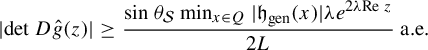 $$ \begin{align*}|\!\det D\hat{g}(z)|\geq\frac{ \sin \theta_{\mathcal{S}}\min_{x\in Q} |\mathfrak{h}_{\mathrm{gen}}(x)|\lambda e^{2\lambda {\operatorname{Re}}\ {z}}}{2 L}\ \text{a.e.}\\[-3.6pc] \end{align*} $$
Next we need the Misiurewicz type Lemma 4 which in this case is expressed as follows.
Lemma 16 Let $D\mathcal{Z}^n_{\mathrm{gen}}$
be the generarized Zorich map and
$D\mathcal{Z}^n_{\mathrm{gen}}$
be the generarized Zorich map and $\mathfrak{h}_{\mathrm{gen}}$
,
$\mathfrak{h}_{\mathrm{gen}}$
, $\theta_{\mathcal{S}}$
be the bi-Lipschitz map and the constant we used in the construction of that Zorich map. Then
$\theta_{\mathcal{S}}$
be the bi-Lipschitz map and the constant we used in the construction of that Zorich map. Then
 $$ \begin{align*}\det(D\mathcal{Z}^n_{\mathrm{gen}}(x))\geq \bigg(\frac{\lambda\min_{x\in Q}|\mathfrak{h}_{\mathrm{gen}}(x)|\sin \theta_{\mathcal{S}}}{L^5}\bigg)^n\frac{1}{\lambda^3}|( p \circ \mathcal{Z}_{\mathrm{gen}}^{n})(x)|^3\ \text{a.e.}\end{align*} $$
Proof. Again the only difference is in obtaining a lower bound for the determinant $\det D\mathcal {Z}_{\mathrm {gen}}(x)$
. Define
$\det D\mathcal {Z}_{\mathrm {gen}}(x)$
. Define
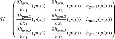 $$ \begin{align*}\mathcal{H}=\begin{pmatrix} \dfrac{\partial h_{\mathrm{gen},1}}{\partial x_1}(p(x))&\dfrac{\partial h_{\mathrm{gen},1}}{\partial x_2}(p(x))&h_{\mathrm{gen},1}(p(x))\\[8pt] \dfrac{\partial h_{\mathrm{gen},2}}{\partial x_1}(p(x))&\dfrac{\partial h_{\mathrm{gen},2}}{\partial x_2}(p(x))&h_{\mathrm{gen},2}(p(x))\\[8pt] \dfrac{\partial h_{\mathrm{gen},3}}{\partial x_1}(p(x))&\dfrac{\partial h_{\mathrm{gen},3}}{\partial x_2}(p(x))&h_{\mathrm{gen},3}(p(x)) \end{pmatrix}\end{align*} $$
and set
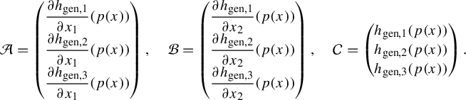 $$ \begin{align*}\mathcal{A}=\begin{pmatrix} \dfrac{\partial h_{\mathrm{gen},1}}{\partial x_1}(p(x))\\ \dfrac{\partial h_{\mathrm{gen},2}}{\partial x_1}(p(x))\\ \dfrac{\partial h_{\mathrm{gen},3}}{\partial x_1}(p(x)) \end{pmatrix},\quad \mathcal{B}=\begin{pmatrix} \dfrac{\partial h_{\mathrm{gen},1}}{\partial x_2}(p(x))\\ \dfrac{\partial h_{\mathrm{gen},2}}{\partial x_2}(p(x))\\ \dfrac{\partial h_{\mathrm{gen},3}}{\partial x_2}(p(x))\end{pmatrix},\quad\mathcal{C}=\begin{pmatrix} h_{\mathrm{gen},1}(p(x))\\ h_{\mathrm{gen},2}(p(x))\\ h_{\mathrm{gen},3}(p(x)) \end{pmatrix}. \end{align*} $$
Then $\det \mathcal {H}=\langle \mathcal {A}\times \mathcal {B}, \mathcal {C}\rangle =|\mathcal {A}\times \mathcal {B}||\mathcal {C}| \cos \phi ,$
where
$\det \mathcal {H}=\langle \mathcal {A}\times \mathcal {B}, \mathcal {C}\rangle =|\mathcal {A}\times \mathcal {B}||\mathcal {C}| \cos \phi ,$
where $\phi $
is the angle between
$\phi $
is the angle between $\mathcal {A}\times \mathcal {B}$
and
$\mathcal {A}\times \mathcal {B}$
and $\mathcal {C}$
. Using the fact that
$\mathcal {C}$
. Using the fact that $|\mathcal {C}|\geq \lambda \min _{x\in Q}|\mathfrak {h}_{\mathrm {gen}}(x)|$
and
$|\mathcal {C}|\geq \lambda \min _{x\in Q}|\mathfrak {h}_{\mathrm {gen}}(x)|$
and $|\mathcal {A}\times \mathcal {B}|\geq {1}/{L^2}$
, together with the non-tangential position vector property, we can show that
$|\mathcal {A}\times \mathcal {B}|\geq {1}/{L^2}$
, together with the non-tangential position vector property, we can show that
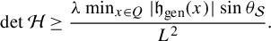 $$ \begin{align*} \det\mathcal{H}\geq \frac{\lambda \min_{x\in Q}|\mathfrak{h}_{\mathrm{gen}}(x)|\sin \theta_{\mathcal{S}} }{L^2}. \end{align*} $$
Hence
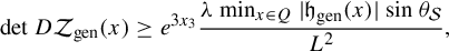 $$ \begin{align*} \det D\mathcal{Z}_{\mathrm{gen}}(x)\geq e^{3x_3}\frac{\lambda \min_{x\in Q}|\mathfrak{h}_{\mathrm{gen}}(x)|\sin \theta_{\mathcal{S}}}{L^2}, \end{align*} $$
and the rest follows in exactly the same way as in the proof of Lemma 4.
Versions of Lemmas 5–10 now follow with only slight modifications of their proofs. Hence, the proof of Theorem 4 now follows with the same arguments as the proof of Theorem 1. Let us briefly sketch how all this should work.
Lemma 17
-
(a) There are
$\delta>0 $
and
$c>0$
such that for all
$x\in C_{\delta }$
, where
$C_{\delta }$
is the cylinder around
$x_3$
-axis with
$\delta $
radius, we have that
$p_3(\mathcal {Z}_{\mathrm {gen}}(x))>p_3(x)+c$
. -
(b) For
$\delta $
as in (a) and for every
$x\in C_{\delta }$
, with
$p(x)\not =(0,0)$
, there is an
$n\in \mathbb {N}$
such that
$\mathcal {Z}_{\mathrm {gen}}^n(x)\not \in C_{\delta }$
.


Proof. The proof of (a) follows that of Lemma 5 word for word. For (b) again the proof is almost the same. The difference here is the lower bound for the angle $\theta $
used in the proof of Lemma 5: instead of
$\theta $
used in the proof of Lemma 5: instead of ${\pi }/{4}$
it is now some constant greater than
${\pi }/{4}$
it is now some constant greater than $0$
.
$0$
.
Lemma 18 Assume $\lambda>{L^5}/({\min _{x\in Q}|\mathfrak {h}_{\mathrm {gen}}(x)|\sin \theta _{\mathcal {S}}})$
. Let
$\lambda>{L^5}/({\min _{x\in Q}|\mathfrak {h}_{\mathrm {gen}}(x)|\sin \theta _{\mathcal {S}}})$
. Let $V\subset \mathbb {R}^3$
be a connected set with
$V\subset \mathbb {R}^3$
be a connected set with $m(V)>0$
and whose iterates do not intersect any of the planes
$m(V)>0$
and whose iterates do not intersect any of the planes $x_1=\pm x_2+2k\lambda $
,
$x_1=\pm x_2+2k\lambda $
, $k\in \mathbb {Z}$
. Suppose also that there is a sequence of integers
$k\in \mathbb {Z}$
. Suppose also that there is a sequence of integers $n_j>0$
with
$n_j>0$
with $\mathcal {Z}_{\mathrm {gen}}^{n_j}(V)\cap C_a=\emptyset $
, where
$\mathcal {Z}_{\mathrm {gen}}^{n_j}(V)\cap C_a=\emptyset $
, where $C_a$
is a cylinder around the
$C_a$
is a cylinder around the $x_3$
-axis of any radius
$x_3$
-axis of any radius $a>0$
. Then
$a>0$
. Then $m(\mathcal {Z}_{\mathrm {gen}}^{n_j}(V))\to \infty $
as
$m(\mathcal {Z}_{\mathrm {gen}}^{n_j}(V))\to \infty $
as $n_j\to \infty $
, where m is the three-dimensional Lebesgue measure.
$n_j\to \infty $
, where m is the three-dimensional Lebesgue measure.
In the same way, as for the Zorich map defined using spheres, we can define the surfaces $S_n$
and
$S_n$
and $K_n$
lying inside the rectangle beams
$K_n$
lying inside the rectangle beams $B_{(0,0)}$
and
$B_{(0,0)}$
and $B_{(0,-1)}$
, respectively. Again those surfaces, together with the plane
$B_{(0,-1)}$
, respectively. Again those surfaces, together with the plane $x_3=0$
and the boundaries of the beams, define sets of finite volume.
$x_3=0$
and the boundaries of the beams, define sets of finite volume.
The next three lemmas are those corresponding to Lemmas 7–9, respectively. Their proofs follow the proofs of the lemmas we just mentioned almost word for word and are therefore omitted.
Lemma 19 Let $I_n$
be the volume that the surface
$I_n$
be the volume that the surface $S_n$
encloses together with the plane
$S_n$
encloses together with the plane $x_3=0$
and inside the beam
$x_3=0$
and inside the beam $B_{(0,0)}$
. Then
$B_{(0,0)}$
. Then $I_n$
is finite for all
$I_n$
is finite for all $n\in \mathbb {N}$
. Furthermore, if
$n\in \mathbb {N}$
. Furthermore, if $T_n:=I_{n+1}-I_n$
is the volume between
$T_n:=I_{n+1}-I_n$
is the volume between $S_n$
and
$S_n$
and $S_{n+1}$
then
$S_{n+1}$
then $T_n$
is a decreasing sequence.
$T_n$
is a decreasing sequence.
Lemma 20 Assume $\lambda>{L^5}/({\min _{x\in Q}|\mathfrak {h}_{\mathrm {gen}}(x)|\sin \theta _{\mathcal {S}}})$
. Let V be a connected subset of
$\lambda>{L^5}/({\min _{x\in Q}|\mathfrak {h}_{\mathrm {gen}}(x)|\sin \theta _{\mathcal {S}}})$
. Let V be a connected subset of $\mathbb {R}^3$
with
$\mathbb {R}^3$
with $m(V)>0$
and such that
$m(V)>0$
and such that $\mathcal {Z}_{\mathrm {gen}}^n(V)$
does not intersect any of the planes
$\mathcal {Z}_{\mathrm {gen}}^n(V)$
does not intersect any of the planes $x_1=\pm x_2+2k\lambda $
,
$x_1=\pm x_2+2k\lambda $
, $k\in \mathbb {Z}$
, for all
$k\in \mathbb {Z}$
, for all $n\in \mathbb {N}$
. Then
$n\in \mathbb {N}$
. Then $\mathcal {Z}_{\mathrm {gen}}^n(V)$
visits infinitely often one of the two rectangle beams
$\mathcal {Z}_{\mathrm {gen}}^n(V)$
visits infinitely often one of the two rectangle beams $B_{(0,0)}$
,
$B_{(0,0)}$
, $B_{(0,-1)}$
, that have the
$B_{(0,-1)}$
, that have the $x_3$
-axis in their boundary.
$x_3$
-axis in their boundary.
Lemma 21 Assume $\lambda>({L^5}/({\min _{x\in Q}|\mathfrak {h}_{\mathrm {gen}}(x)|\sin \theta _{\mathcal {S}}}))$
. Let V be a connected set of
$\lambda>({L^5}/({\min _{x\in Q}|\mathfrak {h}_{\mathrm {gen}}(x)|\sin \theta _{\mathcal {S}}}))$
. Let V be a connected set of $\mathbb {R}^3$
with
$\mathbb {R}^3$
with $m(V)>0$
and such that
$m(V)>0$
and such that $\mathcal {Z}_{\mathrm {gen}}^n(V)$
does not intersect any of the planes
$\mathcal {Z}_{\mathrm {gen}}^n(V)$
does not intersect any of the planes $x_1=\pm x_2+2k\lambda $
,
$x_1=\pm x_2+2k\lambda $
, $k\in \mathbb {Z}$
for all
$k\in \mathbb {Z}$
for all $n\in \mathbb {N}$
. Suppose that there is an
$n\in \mathbb {N}$
. Suppose that there is an $N_0\in \mathbb {N}$
such that
$N_0\in \mathbb {N}$
such that $\mathcal {Z}_{\mathrm {gen}}^n(V)\subset B_{(0,0)}$
, for all
$\mathcal {Z}_{\mathrm {gen}}^n(V)\subset B_{(0,0)}$
, for all $n>N_0$
. Then for all
$n>N_0$
. Then for all $M>0$
and
$M>0$
and $\varepsilon>0$
there exist some
$\varepsilon>0$
there exist some $n_0>N_0$
and a point
$n_0>N_0$
and a point $x\in \mathcal {Z}_{\mathrm {gen}}^{n_0}(V)$
such that
$x\in \mathcal {Z}_{\mathrm {gen}}^{n_0}(V)$
such that $p_3(x)>M$
and
$p_3(x)>M$
and $d(x,x_3\text {-axis})<\varepsilon $
, where d is the euclidean distance.
$d(x,x_3\text {-axis})<\varepsilon $
, where d is the euclidean distance.
The next lemma is the analogue of Lemma 10 in this new setting.
Lemma 22 Let $y_1,y_2\in B(0,r)$
, where
$y_1,y_2\in B(0,r)$
, where $r>0$
. Then for all
$r>0$
. Then for all $n\in \mathbb {N}$
it is true that
$n\in \mathbb {N}$
it is true that
 $$ \begin{align*}|\mathcal{Z}_{\mathrm{gen}}^n(y_1)-\mathcal{Z}_{\mathrm{gen}}^n(y_2)|\leq \bigg(\frac{\sqrt{L^2+\lambda^2}}{\lambda}\bigg)^nE_{\lambda}(r)\cdots E_{\lambda}^n(r)|y_1-y_2|,\end{align*} $$
where $E_{\lambda }$
denotes the exponential map
$E_{\lambda }$
denotes the exponential map $\lambda e^x$
.
$\lambda e^x$
.
Proof. The proof follows the proof of Lemma 10 almost word for word. Note, however, that $\mathcal {A}$
,
$\mathcal {A}$
, $\mathcal {B}$
,
$\mathcal {B}$
, $\mathcal {C}$
are not orthogonal. Still, when estimating
$\mathcal {C}$
are not orthogonal. Still, when estimating $|D\mathcal {Z}_{\mathrm {gen}}(x_1,x_2,0)|$
(see the proof of Lemma 10) we can argue as follows:
$|D\mathcal {Z}_{\mathrm {gen}}(x_1,x_2,0)|$
(see the proof of Lemma 10) we can argue as follows:
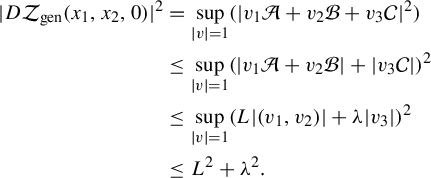 $$ \begin{align*} |D\mathcal{Z}_{\mathrm{gen}}(x_1,x_2,0)|^2&=\sup_{|v|=1}(|v_1\mathcal{A}+v_2\mathcal{B}+v_3\mathcal{C}|^2)\\ &\leq\sup_{|v|=1}(|v_1\mathcal{A}+v_2\mathcal{B}|+|v_3\mathcal{C}|)^2\\ &\leq\sup_{|v|=1}(L|(v_1,v_2)|+\lambda|v_3|)^2\\ &\leq L^2+\lambda^2. \end{align*} $$
We also note that to argue here as in the last few lines of the proof of Lemma 10 we use the two conditions in equation (7.1).
Proof Proof of Theorem 4
Let V be any open and connected set of $\mathbb {R}^3$
. Assuming that
$\mathbb {R}^3$
. Assuming that
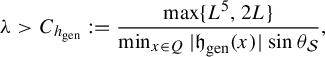 $$ \begin{align*} \lambda>C_{h_{\mathrm{gen}}}:=\frac{\max \{L^5,2 L\}}{\min_{x\in Q}|\mathfrak{h}_{\mathrm{gen}}(x)|\sin \theta_{\mathcal{S}}}, \end{align*} $$
we want to show that $\mathcal {Z}^n_{\mathrm {gen}}(V)$
intersects one of the planes that belong to the Julia set for some n and thus V itself intersects the Julia set.
$\mathcal {Z}^n_{\mathrm {gen}}(V)$
intersects one of the planes that belong to the Julia set for some n and thus V itself intersects the Julia set.
The proof now proceeds in the same way as the proof of Theorem 1. We consider the same two cases.
-
(i) The iterates
$\mathcal {Z}^n_{\mathrm {gen}}(V)$
do not eventually stay inside the beam
$B_{(0,0)}\cup B_{(0,-1)}$
. In this case the proof is the same almost word for word. -
(ii) The iterates
$\mathcal {Z}^n_{\mathrm {gen}}(V)$
eventually stay inside
$B_{(0,0)}\cup B_{(0,-1)}$
. The idea in this case will be the same. We leave the details, which will be slightly different, to the interested reader.


8 Questions and remarks
As we have already seen, the Zorich maps resemble the exponential family in many ways. The literature on exponential dynamics is vast and there are many striking phenomena. It is expected that Zorich maps, given the higher-dimensional setting and their greater flexibility, should have an even more intricate nature. In this section we will mention some problems that require further study.
8.1 Dynamics for different values of
$\lambda $

We saw in Theorem 1 that when $\lambda $
is large enough the Julia set of the Zorich map is the whole of
$\lambda $
is large enough the Julia set of the Zorich map is the whole of $\mathbb {R}^3$
, assuming that
$\mathbb {R}^3$
, assuming that $\nu $
is large enough. It is interesting to ask what happens when the scale factor
$\nu $
is large enough. It is interesting to ask what happens when the scale factor $\lambda $
is not large. In that case we do not have enough expansion in the sense of Lemma 4 in order for our argument to work. Nonetheless, it seems that the dynamics in this case is also chaotic. We therefore pose the following question.
$\lambda $
is not large. In that case we do not have enough expansion in the sense of Lemma 4 in order for our argument to work. Nonetheless, it seems that the dynamics in this case is also chaotic. We therefore pose the following question.
Question 1 Let $\lambda>0$
. Does there always exist a constant
$\lambda>0$
. Does there always exist a constant $c_\lambda $
depending on
$c_\lambda $
depending on $\lambda $
such that for all
$\lambda $
such that for all $\nu>c_\lambda $
the Julia set
$\nu>c_\lambda $
the Julia set $\mathcal {J}(\mathcal {Z}_\nu )$
is the whole of
$\mathcal {J}(\mathcal {Z}_\nu )$
is the whole of $\mathbb {R}^3$
?
$\mathbb {R}^3$
?
We can even pose this question in the complex plane. If we rescale the complex exponential family we obtain the maps
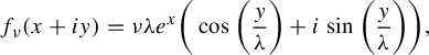 $$ \begin{align*}f_\nu(x+iy)=\nu\lambda e^x \bigg(\cos\bigg(\frac{y}{\lambda}\bigg)+i\sin\bigg(\frac{y}{\lambda}\bigg)\bigg),\end{align*} $$
for $\lambda>0$
and
$\lambda>0$
and $\nu \in \mathbb {R}$
. Note that for
$\nu \in \mathbb {R}$
. Note that for $\lambda =1$
we get the exponential family. Of course those maps are no longer holomorphic but they are quasiregular and we can define their Julia set. A similar approach to that used for the Zorich maps should give us that the Julia set of those maps for
$\lambda =1$
we get the exponential family. Of course those maps are no longer holomorphic but they are quasiregular and we can define their Julia set. A similar approach to that used for the Zorich maps should give us that the Julia set of those maps for $\lambda $
large enough and
$\lambda $
large enough and $\nu>c^{\prime }_{\lambda }$
is the entire complex plane, with
$\nu>c^{\prime }_{\lambda }$
is the entire complex plane, with $c^{\prime }_{\lambda }$
constant depending on
$c^{\prime }_{\lambda }$
constant depending on $\lambda $
. But we can pose the following question.
$\lambda $
. But we can pose the following question.
Question 2 Let $\lambda>0$
. Assuming that
$\lambda>0$
. Assuming that $\nu>c^{\prime }_{\lambda }$
, is
$\nu>c^{\prime }_{\lambda }$
, is $\mathcal {J}(f_\nu )$
the whole complex plane?
$\mathcal {J}(f_\nu )$
the whole complex plane?
Closely related to the above question and worth mentioning here is the paper [Reference Comdühr, Evdoridou and Sixsmith7] where the authors study families of functions like $f_\nu $
in the complex plane. The functions they study are not necessarily quasiregular. However, their results show that if we choose a
$f_\nu $
in the complex plane. The functions they study are not necessarily quasiregular. However, their results show that if we choose a $\lambda>0$
then for small values of
$\lambda>0$
then for small values of $\nu $
the Julia set of
$\nu $
the Julia set of $f_\nu $
is a ‘Cantor bouquet’.
$f_\nu $
is a ‘Cantor bouquet’.
8.2 Measurable dynamics of Zorich maps
In this subsection we assume that $\nu =1$
and
$\nu =1$
and $\lambda $
is as in Theorem 1. We will make some remarks on the Lebesgue measure of some sets. First we need to introduce symbolic dynamics. In order to do that we partition
$\lambda $
is as in Theorem 1. We will make some remarks on the Lebesgue measure of some sets. First we need to introduce symbolic dynamics. In order to do that we partition $\mathbb {R}^3$
into the rectangular beams
$\mathbb {R}^3$
into the rectangular beams
 $$ \begin{align*}T_{(i,j)}=T_{(0,0)}+2i(\lambda,\lambda,0)+2j(\lambda,-\lambda,0),\end{align*} $$
where $i,j\in \mathbb {Z}$
and
$i,j\in \mathbb {Z}$
and
 $$ \begin{align*}\begin{split}T_{(0,0)}&=B_{(0,0)}\cup B_{(0,-1)}\cup\{(x_1,x_2,x_3):x_1=x_2-2\lambda, -2\lambda< x_1\leq 0\}\\ &\quad \cup\{(x_1,x_2,x_3):x_1=-x_2+2\lambda, 0\leq x_1< 2\lambda\}\\ &\quad \cup\{(x_1,x_2,x_3):x_1=x_2, -\lambda< x_1< \lambda\}.\end{split}\end{align*} $$
For each point $x\in \mathbb {R}^3$
we associate a sequence on
$x\in \mathbb {R}^3$
we associate a sequence on $\mathbb {Z}\times \mathbb {Z}$
,
$\mathbb {Z}\times \mathbb {Z}$
, $S(x):=(s_1,s_2,\ldots )$
, which we call its itinerary, and the
$S(x):=(s_1,s_2,\ldots )$
, which we call its itinerary, and the $s_k=(s_{k,1},s_{k,2})$
are chosen such that
$s_k=(s_{k,1},s_{k,2})$
are chosen such that $\mathcal {Z}^k(x)\in T_{s_k}$
. We denote the space of all sequences by
$\mathcal {Z}^k(x)\in T_{s_k}$
. We denote the space of all sequences by $\Sigma $
, so S is a map from
$\Sigma $
, so S is a map from $\mathbb {R}^3$
to
$\mathbb {R}^3$
to $\Sigma $
. This procedure of course can be done to the exponential map in a similar manner. Consider now the set of all points with a given itinerary
$\Sigma $
. This procedure of course can be done to the exponential map in a similar manner. Consider now the set of all points with a given itinerary $(s_1,s_2,\ldots )$
, namely the set
$(s_1,s_2,\ldots )$
, namely the set
 $$ \begin{align*}\{x\in\mathbb{R}^3:S(x)=(s_1,s_2,\ldots)\}.\end{align*} $$
Ghys, Goldberg and Sullivan in [Reference Ghys, Goldberg and Sullivan17] proved that the analogous set for the exponential map has Lebesgue measure zero. With a bit more work we can see that in our proof of Theorem 1 we have actually proved the same result for the Zorich maps. Phrasing it in the same way as in [Reference Ghys, Goldberg and Sullivan17], we have proved the following result.
Theorem 7 The fibres of the map S have Lebesgue measure zero.
Proof. Let V be a set with $m(V)>0$
and where all points in V have the same itinerary s. Remember that the planes
$m(V)>0$
and where all points in V have the same itinerary s. Remember that the planes $x_1=\pm x_2$
together with their parallel translates form a forward invariant set so any point in V which lands on one of those planes stays on those planes. Those points will have zero Lebesgue measure since the planes have zero Lebesgue measure and quasiregular maps have Luzin’s N property (see [Reference Rickman28, I.Proposition 4.14]). Hence, we can assume that V does not contain such points and it always stays on the interior of the square beams under iteration. Thus we find ourselves in the same two cases as in the proof of Theorem 1. Note here that Lemmas 6 and 8 require the set V to be connected. However, it is easy to see in their proofs that this hypothesis can be weakened to all points in V having the same itinerary, which is exactly what we have here.
$x_1=\pm x_2$
together with their parallel translates form a forward invariant set so any point in V which lands on one of those planes stays on those planes. Those points will have zero Lebesgue measure since the planes have zero Lebesgue measure and quasiregular maps have Luzin’s N property (see [Reference Rickman28, I.Proposition 4.14]). Hence, we can assume that V does not contain such points and it always stays on the interior of the square beams under iteration. Thus we find ourselves in the same two cases as in the proof of Theorem 1. Note here that Lemmas 6 and 8 require the set V to be connected. However, it is easy to see in their proofs that this hypothesis can be weakened to all points in V having the same itinerary, which is exactly what we have here.
The first case now of Theorem 1 is exactly the same. Assuming that points in V have an itinerary in which we can find a subsequence $s_{n_k}$
with
$s_{n_k}$
with $s_{n_k}\not =(0,0)$
, we arrive at a contradiction due to the fact that
$s_{n_k}\not =(0,0)$
, we arrive at a contradiction due to the fact that $m(V)>0$
.
$m(V)>0$
.
In the second case we assume that the itinerary of points in V is eventually $0$
, and without loss of generality in fact equal to
$0$
, and without loss of generality in fact equal to $(0,0,\ldots )$
. We may assume that all points in V are density points since by Lebesgue’s density theorem this is true for almost all points. Thus if
$(0,0,\ldots )$
. We may assume that all points in V are density points since by Lebesgue’s density theorem this is true for almost all points. Thus if $x\in V$
then we know that
$x\in V$
then we know that
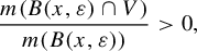 $$ \begin{align*} \frac{m(B(x,\varepsilon)\cap V)}{m(B(x,\varepsilon))}>0, \end{align*} $$
for all $\varepsilon>0$
.
$\varepsilon>0$
.
We now claim that $m(B(x,\varepsilon )\cap V)>0$
, for all
$m(B(x,\varepsilon )\cap V)>0$
, for all $\varepsilon>0$
small enough, if and only if
$\varepsilon>0$
small enough, if and only if $m(B(\mathcal {Z}(x),\varepsilon )\cap \mathcal {Z}(V))>0$
for all
$m(B(\mathcal {Z}(x),\varepsilon )\cap \mathcal {Z}(V))>0$
for all $\varepsilon>0$
small enough. Indeed, this follows by Lusin’s N property and the fact that the Zorich map is locally invertible in
$\varepsilon>0$
small enough. Indeed, this follows by Lusin’s N property and the fact that the Zorich map is locally invertible in $\mathcal {Z}(V)$
.
$\mathcal {Z}(V)$
.
This implies that all points in $\mathcal {Z}^n(V)$
have the property
$\mathcal {Z}^n(V)$
have the property $m(B(y,\varepsilon )\cap \mathcal {Z}^n(V))>0$
for all
$m(B(y,\varepsilon )\cap \mathcal {Z}^n(V))>0$
for all $\varepsilon>0$
small enough. Hence, by Lemma 9, we may assume that x lies in
$\varepsilon>0$
small enough. Hence, by Lemma 9, we may assume that x lies in $A_1$
(otherwise just consider an iterate of V and rename it V) and fix a small
$A_1$
(otherwise just consider an iterate of V and rename it V) and fix a small $\varepsilon $
so that
$\varepsilon $
so that
 $$ \begin{align*}U:=B(x, \varepsilon)\cap V \subset A_1.\end{align*} $$
We can now repeat the argument in the proof of the second case of Theorem 1 and conclude that there is a subsequence $n_j$
with
$n_j$
with $\mathcal {Z}^{n_j}(U)\subset A_2\cup A_3$
but
$\mathcal {Z}^{n_j}(U)\subset A_2\cup A_3$
but $m(\mathcal {Z}^{n_j}(U))\to \infty $
, which is a contradiction due to the fact that
$m(\mathcal {Z}^{n_j}(U))\to \infty $
, which is a contradiction due to the fact that $m(A_2\cup A_3)<\infty $
.
$m(A_2\cup A_3)<\infty $
.
Closely related is the question of the typical behaviour of an orbit of the exponential map. Lyubich in [Reference Lyubich21] proved that for Lebesgue almost all points of the complex plane the limit set of their orbit $E^n(z)$
is the orbit of
$E^n(z)$
is the orbit of $0$
,
$0$
, $\{E^n(0)\}_{n\in \mathbb {N}}$
plus
$\{E^n(0)\}_{n\in \mathbb {N}}$
plus $\infty $
. Thus a typical point will follow closely the orbit of
$\infty $
. Thus a typical point will follow closely the orbit of $0$
for some time and then ‘break off’ for some iterates until it goes back to following the orbit of
$0$
for some time and then ‘break off’ for some iterates until it goes back to following the orbit of $0$
for more iterates this time. Hence, almost all points in the complex plane belong to the bungee set of the exponential map (see [Reference Osborne and Sixsmith26]), namely the set of points that neither escape to infinity nor remain bounded under iteration. The bungee set can be also defined for quasiregular maps (see [Reference Nicks and Sixsmith24]). So we pose the following question.
$0$
for more iterates this time. Hence, almost all points in the complex plane belong to the bungee set of the exponential map (see [Reference Osborne and Sixsmith26]), namely the set of points that neither escape to infinity nor remain bounded under iteration. The bungee set can be also defined for quasiregular maps (see [Reference Nicks and Sixsmith24]). So we pose the following question.
Question 3 What is the typical behaviour of an orbit of a point $x\in \mathbb {R}^3$
under the Zorich map? Do almost all points belong to the bungee set?
$x\in \mathbb {R}^3$
under the Zorich map? Do almost all points belong to the bungee set?
Another interesting question that was answered by Lyubich in the same paper is that of ergodicity of the exponential. Ergodicity here means that there is no partition of the plane into two invariant sets of positive Lebesgue measure. We have the following theorem.
Theorem 8 (Lyubich [Reference Lyubich21]) $E(z)$
is not ergodic.
$E(z)$
is not ergodic.
In the same sense we can pose the following question.
Question 4 Is the Zorich map $\mathcal {Z}$
ergodic?
$\mathcal {Z}$
ergodic?
8.3 Indecomposable continua in Zorich maps
Another fascinating and well-studied phenomenon in exponential dynamics is the presence of indecomposable continua in the dynamic plane. It was Devaney in [Reference Devaney9] who first studied such sets. The way to construct them in the complex plane is as follows. Consider the strip
 $$ \begin{align*} S=\{z\in\mathbb{C}:0\leq{\operatorname{Im}}\ z \leq \pi\}. \end{align*} $$
Now take any $\kappa>1/e$
and consider the set
$\kappa>1/e$
and consider the set
 $$ \begin{align*} \Lambda:=\{z\in\mathbb{C}:E_{\kappa}^n(z)\in S \ \text{for all}\ n\in\mathbb{N}\}. \end{align*} $$
By suitably compactifying this set, Devaney shows that we obtain a curve that accumulates everywhere on itself but does not separate the plane. By applying a theorem due to Curry, [Reference Curry8, Theorem 8], he then concludes that this curve must be an indecomposable continuum.
Assuming that $\nu =1$
, we can try and construct a similar set in the case of Zorich maps. The role of the strip S is now played by the rectangular beam
$\nu =1$
, we can try and construct a similar set in the case of Zorich maps. The role of the strip S is now played by the rectangular beam $\overline {B_{(0,0)}}$
. Thus we can consider the set
$\overline {B_{(0,0)}}$
. Thus we can consider the set
 $$ \begin{align*} \Lambda_{\mathcal{Z}}:=\{x\in\mathbb{R}^3:\mathcal{Z}^n(x)\in \overline{B_{(0,0)}}, \ \text{for all}\ n\in\mathbb{N}\}. \end{align*} $$
We can also, just like Devaney, suitably compactify this set and obtain a surface ( $\Gamma $
, say) that accumulates everywhere on itself. However, Curry’s criterion is no longer available in this higher-dimensional setting, so Devaney’s argument does not work here.
$\Gamma $
, say) that accumulates everywhere on itself. However, Curry’s criterion is no longer available in this higher-dimensional setting, so Devaney’s argument does not work here.
Question 5 Is $\Gamma $
an indecomposable continuum?
$\Gamma $
an indecomposable continuum?
If the answer to the above question is yes we can then consider the same continua for different values of $\nu $
. Let us call these continua
$\nu $
. Let us call these continua $\Gamma _{\nu _1}$
and
$\Gamma _{\nu _1}$
and $\Gamma _{\nu _2}$
, with
$\Gamma _{\nu _2}$
, with $\nu _1$
,
$\nu _1$
, $\nu _2\geq 1$
.
$\nu _2\geq 1$
.
Question 6 If $\nu _1\not =\nu _2$
are
$\nu _1\not =\nu _2$
are $\Gamma _{\nu _1}$
and
$\Gamma _{\nu _1}$
and $\Gamma _{\nu _2}$
homeomorphic?
$\Gamma _{\nu _2}$
homeomorphic?
Let us also remark here that the points in the set $\Lambda _{\mathcal {Z}}$
all have the same itinerary, so by the results of the previous subsection we have that the three-dimensional Lebesgue measure of this set is zero.
$\Lambda _{\mathcal {Z}}$
all have the same itinerary, so by the results of the previous subsection we have that the three-dimensional Lebesgue measure of this set is zero.
Finally, let us mention [Reference Devaney and Jarque12] where the authors prove the existence of many more indecomposable continua in the dynamical plane of the exponential map and ask many more questions. Such considerations also make sense for Zorich maps.
Acknowledgements
I would like to thank my supervisor Daniel Nicks for all his help and encouragement while writing this paper. I would also like to thank Alastair Fletcher, Daniel Meyer and the anonymous referee for their questions which led to a more general version of Theorem 4 and the referee for their thoughtful comments which improved the exposition.


 Open access